Strong convergence to two-dimensional alternating Brownian motion processes

Abstract

Flip-flop processes refer to a family of stochastic fluid processes which converge to either a standard Brownian motion (SBM) or to a Markov modulated Brownian motion (MMBM). In recent years, it has been shown that complex distributional aspects of the univariate SBM and MMBM can be studied through the limiting behaviour of flip-flop processes. Here, we construct two classes of bivariate flip-flop processes whose marginals converge strongly to SBMs and are dependent on each other, which we refer to as alternating two-dimensional Brownian motion processes. While the limiting bivariate processes are not Gaussian, they possess desirable qualities, such as being tractable and having a time-varying correlation coefficient function.

Strong convergence, two-dimensional Brownian motion, stochastic fluid processes, flip-flops, time-varying correlation coefficient

2010 Mathematics Subject Classification: Primary: 60F15, 60G50; Secondary: 60G15

1 Introduction

Let $\mathcal{B}=\{B(t)\}_{t\geq 0}$ denote a standard Brownian motion. The construction of discrete-time random walk approximations to $\mathcal{B}$ is a well-known problem initiated by Donsker in [10]. His work dealt with weak approximations, that is, with the convergence of the laws of appropriately scaled random walks to the law of $\mathcal{B}$. A different technique using strong approximations was proposed by Strassen [26], which involved the construction of a probability space where the paths of the scaled random walks were shown to converge uniformly on compact intervals to the path of $\mathcal{B}$. Not only did Strassen’s technique provide an alternative approach to the construction of approximations to $\mathcal{B}$, but it also yielded stronger results: a strongly convergent family of stochastic processes to $\mathcal{B}$ is automatically weakly convergent, while the opposite is not always true. Furthermore, strong convergence allows one to claim convergence of pathwise functionals of the processes.

In this paper we focus on strong approximations to $\mathcal{B}$ and related models, not using discrete-time random walks, but a family of continuous-time stochastic processes which we introduce next.

Definition 1.1.

Consider a family of processes $\{\mathcal{F}_{\lambda}\}_{\lambda>0}=\{\{F_{\lambda}(t)\}_{t\geq 0}\}_{\lambda>0}$, where

$$F_{\lambda}(t):=\sqrt{\lambda}\int_{0}^{t}J_{\lambda}(s)\mathrm{d}s,\quad t\geq 0,$$

and the phase process $\mathcal{J}_{\lambda}=\{J_{\lambda}(t)\}_{t\geq 0}$ denotes a Markov jump process with state space $\mathcal{E}=\{1,-1\}$ and intensity matrix given by

$$\Lambda=\left[\begin{array}[]{rr}-\lambda&\lambda\\ \lambda&-\lambda\end{array}\right].$$ (1.3)

We refer to $\mathcal{F}_{\lambda}$ as the standard flip-flop process.

Intuitively, the process $\mathcal{F}_{\lambda}$ describes the path of a particle in $\mathds{R}$ with finite constant velocity which randomly switches direction at a constant rate. Such a process has been studied in the literature as the uniform transport process [28, 14], and is also a special case of the telegraph process [12, 15] and, more recently, of the flip-flop process [25, 18].

The standard flip-flop process $\mathcal{F}_{\lambda}$ belongs to a larger class of piecewise-linear models modulated by a Markov jump process, called stochastic fluid processes (SFP), for which several first passage results and formulae are available [16]. Even if the behaviour of $\mathcal{F}_{\lambda}$ is somewhat similar to that of a random walk with double-sided exponential increments, notice that changes in direction of $\mathcal{F}^{\lambda}$ happen at random time epochs. In comparison, the discrete-time random walks approximations to $\mathcal{B}$ devised in [10, 26] have inflection points on a deterministic grid. Though this characteristic of $\mathcal{F}_{\lambda}$ may seem inconvenient at first, once a limiting result is established, it actually allows us to translate well-understood results from SFPs into complex second-order models such as the Markov modulated Brownian motion (MMBM), as recently evidenced in [18, 17, 2, 19, 1, 21]. Besides being important objects of study within the matrix-analytic-methods community, both SFPs and MMBMs have been succesfully used to model random systems in queueing theory, risk theory, finance and epidemiology.

The weak convergence of $\mathcal{F}_{\lambda}$ to $\mathcal{B}$ as $\lambda\rightarrow\infty$ was first established in [28]. Through different constructions, it was shown in [14, 23, 24] that $\mathcal{F}_{\lambda}$ also converges strongly to $\mathcal{B}$; that is, they showed the existence of a probability space $(\Omega,\mathscr{F},\mathds{P})$ such that for all $T\geq 0$,

$$\lim_{\lambda\rightarrow\infty}\sup_{0\leq s\leq T}|F_{\lambda}(s)-B(s)|=0\quad\mbox{almost surely}.$$

In order to extend these strong approximations into two-dimensional processes, consider two families of standard flip-flops, $\{\mathcal{F}^{1}_{\lambda}\}$ and $\{\mathcal{F}^{2}_{\lambda}\}$, with corresponding families of phase processes $\{\mathcal{J}_{\lambda}^{1}\}$ and $\{\mathcal{J}_{\lambda}^{2}\}$, living on two probability spaces $(\Omega^{1},\mathscr{F}^{1},\mathds{P}^{1})$ and $(\Omega^{2},\mathscr{F}^{2},\mathds{P}^{2})$, respectively. One can see that, on $(\Omega^{1}\times\Omega^{2},\mathscr{F}^{1}\otimes\mathscr{F}^{2},\mathds{P}^{1}\times\mathds{P}^{2})$, the bivariate process $(\mathcal{F}^{1}_{\lambda},\mathcal{F}^{2}_{\lambda})$ converges strongly to a two-dimensional Brownian motion $(\mathcal{B}^{1},\mathcal{B}^{2})$ as $\lambda\rightarrow\infty$.

The process $\left(\mathcal{F}^{1}_{\lambda},\mathcal{F}^{2}_{\lambda}\right)$ can be redefined such that $\mathcal{F}^{1}_{\lambda}$ and $\mathcal{F}^{2}_{\lambda}$ are jointly modulated by a common phase process, as follows.

Definition 1.2.

Let $\bm{\mathcal{J}}_{\lambda}=\{\bm{J}_{\lambda}(t)\}=\left\{\left(J_{\lambda}^{1}(t),J_{\lambda}^{2}(t)\right)\right\}$ be a Markov jump process on state space $\mathcal{E}^{2}=\{(1,1),(1,-1),(-1,1),(-1,-1)\}$ with the intensity matrix

$$\Lambda\oplus\Lambda=\left[\begin{array}[]{rrrr}-2\lambda&\lambda&\lambda&0\\ \lambda&-2\lambda&0&\lambda\\ \lambda&0&-2\lambda&\lambda\\ 0&\lambda&\lambda&-2\lambda\end{array}\right],$$ (1.8)

where $\oplus$ denotes the Kronecker sum. Let

$$F^{i}_{\lambda}(t):=\sqrt{\lambda}\int_{0}^{t}\pi_{i}\left(\bm{J}_{\lambda}(s)\right)\mathrm{d}s,\quad t\geq 0,i=1,2,$$

where $\pi_{i}:\mathcal{E}^{2}\mapsto\mathcal{E}$ denotes the $i$th coordinate projection. We refer to $\left(\mathcal{F}^{1}_{\lambda},\mathcal{F}^{2}_{\lambda}\right)$ as a standard bivariate flip-flop process, and $\bm{\mathcal{J}}_{\lambda}$ its underlying phase process.

More broadly, we define the following.

Definition 1.3.

A bivariate flip-flop process $\left(\mathcal{G}^{1}_{\lambda},\mathcal{G}^{2}_{\lambda}\right)=\left\{\left({G}^{1}_{\lambda}(t),{G}^{2}_{\lambda}(t)\right)\right\}_{t\geq 0}$ is defined by

$$G^{i}_{\lambda}(t):=\sqrt{\lambda}\int_{0}^{t}\pi_{i}^{*}(\bm{J}_{\lambda}(s))\mathrm{d}s,\quad t\geq 0,$$ (1.9)

where $\bm{\mathcal{J}}_{\lambda}$ is a Markov jump process on $\mathcal{E}^{2}\times\mathcal{S}$, where $\mathcal{S}$ is some finite collection of states, and $\pi_{i}^{*}:\mathcal{E}^{2}\times\mathcal{S}\rightarrow\mathds{R}$, $i\in\{1,2\},$ is such that

$$\pi_{1}^{*}((1,\mathcal{E})\times\mathcal{S}) =\pi_{2}^{*}((\mathcal{E},1)\times\mathcal{S})=1,$$

$$\pi_{1}^{*}((-1,\mathcal{E})\times\mathcal{S}) =\pi_{2}^{*}((\mathcal{E},-1)\times\mathcal{S})=-1.$$

Thus, a bivariate flip-flop process has an underlying phase process $\bm{\mathcal{J}}_{\lambda}$ with a considerably richer structure than that of (1.8), which may be used to produce dependent coordinate processes instead of independent ones. One natural goal is to characterise all possible strong limits for bivariate flip-flop processes and study their dependence structures.

As a step toward that goal, we construct in this paper two families of bivariate flip-flop processes and show that each converges strongly to a process, of which the marginals are standard Brownian motion and the correlation between the two components is a time-varying function. In short, the marginals of the limiting process alternate between synchronising intervals during which they evolve with identical increments to each other, and desynchronising intervals during which they evolve as mirror images of each other. In Section 3 the intervals are exponentially distributed and we call the limiting process a two-dimensional exponentially alternating Brownian motion. In Section 4 the synchronisation and desynchronisation epochs are determined by a continuous-time Markovian arrival process (MAP); we refer to this process as a two-dimensional MAP alternating Brownian motion. We determine the time-varying correlation functions of the limiting processes in Sections 3 and 4, respectively.

From a different perspective, the bivariate flip-flop processes can be seen as a continuous-time analogue of the discrete-time bootstrapping random walk concept proposed in [9, 8]. There, the authors start by constructing a discrete-time random walk from Bernoulli random variables, and then reuse (bootstrap) these random variables to create additional walks; together, the random walks converge weakly to two- or higher-dimensional Brownian motions. In our case, we will start by constructing a continuous-time random walk (standard flip-flop) from exponential random variables, and then reuse them to create an additional continuous-time random walk; together, the random walks (bivariate flip-flop) converge strongly to a two-dimensional process. In one construction, the strong limit is a two-dimensional Brownian motion; in two others, the strong limits are two-dimensional alternating Brownian motion processes.

Another related model is the zig-zag process [6], a multidimensional piecewise deterministic Markov process which behaves in a piecewise linear fashion over time. Changes in direction of the path of a zig-zag process occur according to some space-dependent intensity function, the latter chosen in such a way that the stationary behaviour of the process follows some prespecified distribution. Although flip-flop processes are in fact a space-homogeneous version of the zig-zag processes, their use differ: zig-zag processes are commonly used to implement efficient sampling methods [4, 5], while the goal of flip-flop processes is to explain properties of complex second-order processes.

2 Preliminaries

Our construction of bivariate flip-flops is inspired by [24], and we sketch in this section the construction proposed there for one-dimensional standard flip-flops. The creation in [24] of a family of standard flip-flops $(\mathcal{F}_{\lambda},\mathcal{J}_{\lambda})$, with $\lambda\rightarrow\infty$, relies on inspecting the standard Brownian motion $\mathcal{B}$ at the arrival epochs of a Poisson process, as explained next.

For $\lambda>0$, let $\{\tau^{\lambda}_{k}\}_{k\geq 0}$, with $\tau_{0}^{\lambda}=0$, be the arrival epochs of a Poisson process of intensity $2\lambda$, independent of $\mathcal{B}$. For notational convenience, we omit the superscript $\lambda$ when no ambiguity might arise. Let

$$C_{k}:=B(\tau_{k+1})-B(\tau_{k}),\quad k\geq 0;$$

the sequence $\{C_{k}\}_{k\geq 0}$ has i.i.d. elements with common double exponential distribution of parameter $2\sqrt{\lambda}$ [24, Theorem 2.1], that is, following the density function

$$f(x)=\sqrt{\lambda}\,e^{-2\sqrt{\lambda}\,|x|},\quad x\in\mathds{R}.$$

One can verify that $\{|C_{k}|\}_{k\geq 0}$ and $\{C_{k}/|C_{k}|\}_{k\geq 0}$ are independent i.i.d. sequences where $|C_{k}|\sim\mbox{Exp}(2\sqrt{\lambda})$ and $\mathds{P}\left(C_{k}/|C_{k}|=1\right)=\mathds{P}\left(C_{k}/|C_{k}|=-1\right)=1/2.$

Next, define the epochs $\{\xi_{k}^{\lambda}\}_{k\geq 0}$, which we write $\{\xi_{k}\}_{k\geq 0}$, with $\xi_{0}=0$ by

$${\xi_{k+1}-\xi_{k}:=\lambda^{-1/2}|C_{k}|,}$$

and the process $\mathcal{J}_{\lambda}=\{J_{\lambda}(t)\}_{t\geq 0}$ by

$$J_{\lambda}(t):=C_{k}/|C_{k}|,\quad\mbox{ for }t\in[\xi_{k},\xi_{k+1}),\,k\geq 0.$$ (2.1)

Note that $\mathcal{J}_{\lambda}$ might or might not change states at a given epoch $\xi_{k}$. Let $\{\chi_{k}\}_{k\geq 1}$, $\chi_{0}:=0$, denote the jump times of $\mathcal{J}_{\lambda}$. By the independence properties of $\{|C_{k}|\}_{k\leq 0}$ and $\{C_{k}/|C_{k}|\}_{k\leq 0}$, the elements of $\{\chi_{k+1}-\chi_{k}\}_{k\geq 0}$ are i.i.d. random variables which follow a $\mbox{Geometric}(0.5)$ random sum of exponentials of intensity $2\lambda$. Equivalently, $\chi_{k+1}-\chi_{k}$ is an exponential random variable of intensity $\lambda$. Thus, $\mathcal{J}_{\lambda}$ is a Markov jump process driven by the rate matrix $\left[\begin{matrix}[r]-\lambda&\lambda\\ \lambda&-\lambda\end{matrix}\right]$ and has initial distribution $(1/2,1/2)$.

Intuitively, to see that $\mathcal{F}_{\lambda}=\{F_{\lambda}(t)\}_{t\geq 0}$, defined by

$$F_{\lambda}(t)=\sqrt{\lambda}\int_{0}^{t}J_{\lambda}(s)\mathrm{d}s,$$ (2.2)

approximates $\mathcal{B}$ on $[0,T$], note that $F_{\lambda}(\xi_{k})=B(\tau_{k})$ for $k\geq 0$. Moreover, since $\tau_{k}\sim\mbox{Erlang}(k,2\lambda)$ and $\xi_{k}\sim\mbox{Erlang}(k,2\lambda)$, we have $\mathds{E}(\tau_{k})=\mathds{E}(\xi_{k})$, implying that on average the epochs $\{\tau_{k}\}$ coincide with $\{\xi_{k}\}$. More precisely, Nguyen and Peralta [24] showed that

$$\lim_{\lambda\rightarrow\infty}\max_{k:\tau_{k}^{\lambda},\chi_{k}^{\lambda}<T}|\tau_{k}^{\lambda}-\xi_{k}^{\lambda}| =0\quad\mbox{almost surely,}$$

and furthermore,

$$\lim_{\lambda\rightarrow\infty}\sup_{0\leq s\leq T}|F_{\lambda}(s)-B(s)|=0\quad\mbox{almost surely}.$$ (2.3)

See Figure 1 for a sample path approximation of the standard Brownian motion $\mathcal{B}$ with the flip-flop process $\mathcal{F}_{\lambda}$.

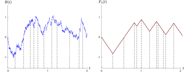
Figure 1: (Left) A sample path of an SBM $\mathcal{B}$. The dashed lines correspond to the arrival epochs $\{\tau_{k}\}_{k\geq 0}$. (Right) An associated sample path of a standard flip-flop $\mathcal{F}_{\lambda}$. The epochs $\{\xi_{k}\}_{k\geq 0}$ are shown with dashed lines. Note the values of $F_{\lambda}(\xi_{k})$ match those of $B(\tau_{k})$.

3 Reflection at exponential times

Here, we construct on a probability space $(\Omega,\mathscr{F},\mathds{P})$ a family of bivariate flip-flops $\{(\mathcal{F}^{1}_{\lambda},\mathcal{F}^{2}_{\lambda})\}_{\lambda\geq 0}$, such that $\{(\mathcal{F}^{1}_{\lambda},\mathcal{F}^{2}_{\lambda})\}$ converges strongly to a so-called two-dimensional exponentially alternating Brownian motion as $\lambda\rightarrow\infty$.

Definition 3.1.

Let $\mathcal{X}=\{X(t)\}_{t\geq 0}$ be a Markov jump process with state space $\{0,1\}$, initial probability $(1,0)$ and intensity matrix

$$\Pi=\left[\begin{array}[]{rr}-\alpha&\alpha\\ \beta&-\beta\end{array}\right],$$ (3.3)

and let $\mathcal{B}$ be a standard Brownian motion. Define $\mathcal{B}^{*}=\{B^{*}(t)\}_{t\geq 0}$ such that

$$B^{*}(t)=\int_{0}^{t}(-1)^{X(s)}\mathrm{d}B(s),\quad t\geq 0.$$ (3.4)

The process $(\mathcal{B},\mathcal{B}^{*})$ is called a two-dimensional exponentially alternating Brownian motion.

In the intervals during which $X(t)=0$, the processes $\mathcal{B}$ and $\mathcal{B}^{*}$ evolve with precisely the same increment; we refer to these periods as synchronising intervals. In intervals during which $X(t)=1$, the increment of one process is the negative of the other; these are desynchronising intervals.

It is important to notice that $(\mathcal{B},\mathcal{B}^{*})$ is not a Gaussian process: for instance, the distribution of $B(t)-B^{*}(t)$ has a point mass at $0$ of size $e^{-\alpha t}$, corresponding to the event $\{X(s)=0\mbox{ for all }0\leq s\leq t\}$. Despite not being Gaussian, $(\mathcal{B},\mathcal{B}^{*})$ is still a process with tractable properties, as we show later in Section 3.2.

3.1 Construction

Let $\mathcal{J}_{\lambda}^{1}=\mathcal{J}_{\lambda}$ and define $\mathcal{J}_{\lambda}^{2}=\{J_{\lambda}^{2}(t)\}_{t\geq 0}$ by

$${J_{\lambda}^{2}(t):=(-1)^{X(t)}J_{\lambda}(t),\quad t\geq 0,}$$

where $\mathcal{J}_{\lambda}=\{J_{\lambda}(t)\}_{t\geq 0}$ is the Markov jump process constructed in (2.1). Then $(\mathcal{J}_{\lambda}^{1},\mathcal{J}_{\lambda}^{2})$ is a Markov jump process with state space

$$\mathcal{E}^{2}=\{(1,1),(1,-1),(-1,1),(-1,-1)\},$$

initial distribution $(1/2,0,0,1/2)$, and has the intensity matrix given by

$$\Pi_{\lambda}=\left[\begin{array}[]{cccc}-\lambda-\alpha&\alpha&0&\lambda\\ \beta&-\lambda-\beta&\lambda&0\\ 0&\lambda&-\lambda-\alpha&\alpha\\ \lambda&0&\beta&-\lambda-\beta\end{array}\right].$$ (3.9)

Indeed, for $j\in\{1,-1\}$, jumps from $(j,1)$ to $(-j,-1)$ are linked to those jumps associated to $\mathcal{J}_{\lambda}$ which happen with rate $\lambda$, while jumps from $(j,1)$ to $(j,-1)$ occur thanks to desynchronisation events which happen with rate $\alpha$. Similar explanations hold for jumps originating from $(j,-1)$.

Define the flip-flop processes $\mathcal{F}^{1}_{\lambda}=\{F_{\lambda}^{1}(t)\}_{t\geq 0}$ and $\mathcal{F}^{2}_{\lambda}=\{F_{\lambda}^{2}(t)\}_{t\geq 0}$ by

$$F^{i}_{\lambda}(t):=\sqrt{\lambda}\int_{0}^{t}J^{i}_{\lambda}(s)\,\mathrm{d}s,\quad i\in\{1,2\},\,t\geq 0.$$

Theorem 3.2.

As $\lambda\rightarrow\infty$, the bivariate flip-flop $(\mathcal{F}^{1}_{\lambda},\mathcal{F}^{2}_{\lambda})$ converges strongly to the process $(\mathcal{B},\mathcal{B}^{*})$; that is, for all $T>0$,

$$\lim_{n\rightarrow\infty}\sup_{0\leq s\leq T}\left\|\left(F^{1}_{\lambda}(s),F^{2}_{\lambda}(s)\right)-\left(B(s),B^{*}(s)\right)\right\|_{\infty}=0,$$ (3.10)

where $\|\cdot\|_{\infty}$ denotes the max–norm in $\mathds{R}^{2}$.

Furthermore, for all $q>0$ there exists $\varepsilon>0$ such that

$$\mathds{P}\left(\sup_{0\leq s\leq T}\left\|\left(F^{1}_{\lambda}(s),F^{2}_{\lambda}(s)\right)-\left(B(s),B^{*}(s)\right)\right\|_{\infty}\geq{\eta_{q,\lambda}}\varepsilon(\log\lambda)\lambda^{-1/4}\right)=o(\lambda^{-q}),$$ (3.11)

where $\eta_{q,\lambda}:=\max(1,2q\log\lambda)$. The term $\eta_{q,\lambda}\varepsilon(\log\lambda)\lambda^{-1/4}$ is said to be the rate of strong convergence of $(\mathcal{F}^{1}_{\lambda},\mathcal{F}^{2}_{\lambda})$ to $(\mathcal{B},\mathcal{B}^{*})$.

Proof.

Note that

$$\sup_{0\leq s\leq T}\left\|\left(F^{1}_{\lambda}(s),F^{2}_{\lambda}(s)\right)-\left(B(s),B^{*}(s)\right)\right\|_{\infty}\leq\sup_{0\leq s\leq T}\left|F^{1}_{\lambda}(s)-B(s)\right|+\sup_{0\leq s\leq T}\left|F^{2}_{\lambda}(s)-B^{*}(s)\right|.$$

Then, (3.10) follows once we prove that $\mathcal{F}^{1}_{\lambda}$ strongly converges to $\mathcal{B}$, and that $\mathcal{F}^{2}_{\lambda}$ strongly converges to $\mathcal{B}^{*}$. The former is a consequence of $\mathcal{F}^{1}_{\lambda}=\mathcal{F}_{\lambda}$, with $\mathcal{F}_{\lambda}$ as defined in (2.2), and the strong convergence (2.3) proved in [24]. In fact, Nguyen and Peralta [24] proved that for all $q>0$ there exists $\varepsilon>0$ such that

$$\mathds{P}\left(\sup_{0\leq s\leq T}|F_{\lambda}(s)-B(s))|\geq\varepsilon(\log\lambda)\lambda^{-1/4}\right)=o(\lambda^{-q});$$ (3.12)

the term $\varepsilon(\log\lambda)\lambda^{-1/4}$ is the rate of strong convergence of $\mathcal{F}_{\lambda}$ to $\mathcal{B}$.

The case of the convergence of $\mathcal{F}^{2}_{\lambda}$ to $\mathcal{B}^{*}$ is more complicated because the synchronisation/desynchronisation events may cause further separation of the paths, in comparison to that of $\mathcal{F}_{\lambda}$ to $\mathcal{B}$. More precisely, let $\{\rho_{k}\}_{k\geq 0}$ be the jump times of $\mathcal{X}$, defined by $\rho_{k+1}:=\inf\{s>\rho_{k}:X(s-)\neq X(s)\}$ with $\rho_{0}=0$. Now, suppose that $\rho_{1}\leq T<\rho_{2}$: then,

$$\sup_{\rho_{1}\leq s\leq T}|F^{2}_{\lambda}(s)-B^{*}(s)| {=\sup_{\rho_{1}\leq s\leq T}\left|F_{\lambda}(\rho_{1})+\left(-F_{\lambda}(s)+F_{\lambda}(\rho_{1})\right)-[B(\rho_{1})+(-B(s)+B(\rho_{1}))]\right|}$$

$${=\sup_{\rho_{1}\leq s\leq T}\left|2F_{\lambda}(\rho_{1})-F_{\lambda}(s)-2B(\rho_{1})+B(s)\right|}$$

$$=\sup_{\rho_{1}\leq s\leq T}|{2}(F_{\lambda}(\rho_{1})-B(\rho_{1}))+(B(s)-F_{\lambda}(s))|$$

$$\leq{2}|F_{\lambda}(\rho_{1})-B(\rho_{1})|+\sup_{\rho_{1}\leq s\leq T}\left|F_{\lambda}(s)-B(s)\right|$$

$$\leq{3}\sup_{0\leq s\leq T}\left|F_{\lambda}(s)-B(s)\right|{.}$$

implying that

$$\sup_{0\leq s\leq T}\left|F^{2}_{\lambda}(s)-B^{*}(s)\right|\leq{3}\sup_{0\leq s\leq T}\left|F_{\lambda}(s)-B(s)\right|.$$

Using recursive arguments, we get the bound for the general case

$$\sup_{0\leq s\leq T}\left|F^{2}_{\lambda}(s)-B^{*}(s)\right| \leq(2R-1)\left[\sup_{0\leq s\leq T}\left|F_{\lambda}(s)-B(s)\right|\right],$$ (3.13)

where $R:=\inf\{k\geq 1:\rho_{k}>T\}$. Equation (3.13) implies that the convergence of $\mathcal{F}^{2}_{\lambda}$ to $\mathcal{B}^{*}$ is slower than that of $\mathcal{F}_{\lambda}$ to $\mathcal{B}$.

To precisely measure its rate of strong convergence, note that since $R$ has a Poissonian tail of parameter $\gamma_{0}T$ with $\gamma_{0}:=\alpha\wedge\beta$; by [11], $\mathds{P}(R>n)=o\left(e^{-n(\log n-\gamma_{0}T)}\right).$ This in turn gives

$$\mathds{P}(R>q\log\lambda)=o\left(\lambda^{-q}\right).$$ (3.14)

Equations (3.12), (3.13) and (3.14) suggest that the rate of strong convergence of $\mathcal{F}_{\lambda}^{2}$ to $\mathcal{B}^{*}$ is $\varepsilon^{*}(\log\lambda)^{2}\lambda^{-1/4}$ where $\varepsilon^{*}:=2\varepsilon q$. Indeed,

$$\mathds{P}\left(\sup_{0\leq s\leq T}|F^{2}_{\lambda}(s)-B^{*}(s)|\geq\varepsilon^{*}(\log\lambda)^{2}\lambda^{-1/4}\right)$$

$$\quad\leq\mathds{P}\left((2R-1)\left[\sup_{0\leq s\leq T}\left|{F}_{\lambda}(s)-B(s)\right|\right]\geq\varepsilon^{*}(\log\lambda)^{2}\lambda^{-1/4}\right)$$

$$\quad\leq\mathds{P}\left((2R-1)\left[\sup_{0\leq s\leq T}\left|{F}_{\lambda}(s)-B(s)\right|\right]\geq\varepsilon^{*}(\log\lambda)^{2}\lambda^{-1/4},R\leq q\log\lambda\right)$$

$$\quad\quad+\mathds{P}(R>q\log\lambda)$$

$$\quad\leq\mathds{P}\left(\sup_{0\leq s\leq T}|F^{1}_{\lambda}(s)-B(s)|\geq\varepsilon(\log\lambda)\lambda^{-1/4}\right)+\mathds{P}(R>q\log\lambda)=o(\lambda^{-q}),$$

and, thus, $\sup_{0\leq s\leq T}\left|F^{2}_{\lambda}(s)-B^{*}(s)\right|$ converges almost surely to $0$.

Finally, the strong convergence rate for the bivariate process $(\mathcal{F}^{1}_{\lambda},\mathcal{F}^{2}_{\lambda})$ follows from taking the maximum between the two strong convergence rates of the marginal processes $\mathcal{F}^{1}_{\lambda}$ and $\mathcal{F}^{2}_{\lambda}$, to $\mathcal{B}$ and $\mathcal{B}^{*}$, respectively. ∎

3.2 Dependence of the limiting process

As previously mentioned, the process $(\mathcal{B},\mathcal{B}^{*})$ is not Gaussian. In this section we examine its dependency structure.

Theorem 3.3.

The correlation coefficient function

$$\mathrm{Corr}(t)=\frac{\mathds{E}\left[B(t)B^{*}(t)\right]-\mathds{E}[B(t)]\mathds{E}[B^{*}(t)]}{\sqrt{\mbox{\emph{Var}}(B(t))}\sqrt{\mbox{\emph{Var}}(B^{*}(t))}}=\frac{\mathds{E}\left[B(t)B^{*}(t)\right]}{t}\quad\mbox{for $t>0$.}$$

of $\mathcal{B}$ and $\mathcal{B}^{*}$ is given by

$$\mathrm{Corr}(t)=\frac{\alpha^{-1}-\beta^{-1}}{\alpha^{-1}+\beta^{-1}}+\frac{2\alpha(1-e^{-t(\alpha+\beta)})}{t(\alpha+\beta)^{2}}.$$ (3.15)

Proof.

Fix $t\geq 0$. Let $M_{s}:=B({t\wedge s})$ and $N_{s}:=B^{*}({t\wedge s})$ for all $s\geq 0$. The processes $\{M_{s}\}_{s\geq 0}$ and $\{N_{s}\}_{s\geq 0}$ are martingales bounded in $L_{2}$, so that [22, Prop. 4.15]

$$\mathds{E}\big{[}B(t)B^{*}(t)\big{]}=\mathds{E}[M_{\infty}N_{\infty}]=\mathds{E}[\langle M,N\rangle_{\infty}],$$

where $\{\langle M,N\rangle_{s}\}_{0\leq s}$ denotes the bracket process of $\{M^{t}_{s}\}_{s\geq 0}$ and $\{N^{t}_{s}\}_{s\geq 0}$ [22, Defn 4.14]. Since $\{N_{s}\}_{s\geq 0}$ admits the stochastic integral representation (3.4), then by [22, Thm 5.4]

$$\mathds{E}[\langle M,N\rangle_{\infty}]=\mathds{E}\left[\int_{0}^{t}(-1)^{X(s)}\mathrm{d}s\right]=\int_{0}^{t}\mathds{E}\left[(-1)^{X(s)}\right]\mathrm{d}s.$$

Straightforward computations show that

$$\mathds{P}(X(s)=0)=\left([1,0]\exp\left(\Pi s\right)\right)_{1} =\frac{\alpha^{-1}}{\alpha^{-1}+\beta^{-1}}+\frac{\alpha}{\alpha+\beta}e^{-s(\alpha+\beta)},$$

$$\mathds{P}(X(s)=1)=\left([1,0]\exp\left(\Pi s\right)\right)_{2} =\frac{\beta^{-1}}{\alpha^{-1}+\beta^{-1}}-\frac{\alpha}{\alpha+\beta}e^{-s(\alpha+\beta)}.$$

Thus,

$$\mathds{E}\big{[}B(t)B^{*}(t)\big{]} =\int_{0}^{t}\mathds{E}\left((-1)^{X(s)}\right)\mathrm{d}s$$

$$=\int_{0}^{t}\frac{\alpha^{-1}-\beta^{-1}}{\alpha^{-1}+\beta^{-1}}+\frac{2\alpha}{\alpha+\beta}e^{-s(\alpha+\beta)}\mathrm{d}s$$

$$=t\frac{\alpha^{-1}-\beta^{-1}}{\alpha^{-1}+\beta^{-1}}+\frac{2\alpha(1-e^{-t(\alpha+\beta)})}{(\alpha+\beta)^{2}}.$$

∎

Remark 3.4.

We observe from Theorem 3.3 that the limiting process $(\mathcal{B},\mathcal{B}^{*})$ has a time-dependent correlation function, which starts in $1$, is strictly decreasing and converges to $(\alpha^{-1}-\beta^{-1})/(\alpha^{-1}+\beta^{-1})$ as $t\rightarrow\infty$. From a modelling perspective, this provides an alternative to classic correlated bivariate Brownian motion models, for which the correlation function remains constant over time.

An analogous construction can be made so that $\mathcal{B}^{*}$ starts in a desynchronized environment, that is, $\mathds{P}(X(0)=1)=1$. A slight modification to the proof of Theorem 3.3 shows that the correlation coefficient for such a construction is given by

$$\mathrm{Corr}(t)=\frac{\alpha^{-1}-\beta^{-1}}{\alpha^{-1}+\beta^{-1}}-\frac{2\beta(1-e^{-t(\alpha+\beta)})}{t(\alpha+\beta)^{2}}.$$

4 Reflection at MAP times

In this section, we construct a flip-flop approximation to a new class of bivariate Brownian motion processes with a more flexible time-dependent correlation function, which we call two-dimensional MAP alternating Brownian motion. They are a generalization of the process in Section 3 as the synchronisation and desynchronisation epochs now occur at arrival epochs of a continuous-time MAP. In continuous time, a MAP of parameters $(\bm{b},C,D)$ is a counting process $\mathcal{K}$ driven by an underlying Markov jump process with initial distribution $\bm{b}$ and intensity matrix $C+D$. The epochs of increase of $\mathcal{K}=\{K(t)\}_{t\geq 0}$ coincide with those jumps epochs which occur due to the intensities of the matrix $D$. See [20] for a detailed exposition on the topic.

Definition 4.1.

Let $\mathcal{K}=\{K(t)\}_{t\geq 0}$ be a continuous-time MAP$(\bm{b},C,D)$, and $\mathcal{B}$ be a standard Brownian motion. Define $\mathcal{B}^{*}=\{B^{*}(t)\}_{t\geq 0}$ such that

$$B^{*}(t)=\int_{0}^{t}(-1)^{K(s)}\mathrm{d}B_{s},\quad t\geq 0.$$

The process $(\mathcal{B},\mathcal{B}^{*})$ is called a two-dimensional MAP alternating Brownian motion.

4.1 Construction

Here, let $\mathcal{J}_{\lambda}^{1}=\mathcal{J}_{\lambda}$ where $\mathcal{J}_{\lambda}$ is defined as in (2.1), and let $\mathcal{J}_{\lambda}^{2}=\{J_{\lambda}^{2}(t)\}_{t\geq 0}$ where

$${J_{\lambda}^{2}(t):=(-1)^{K(t)}J_{\lambda}(t),\quad t\geq 0.}$$

Define the flip-flop processes $\mathcal{F}^{1}_{\lambda}=\{F_{\lambda}^{1}(t)\}_{t\geq 0}$ and $\mathcal{F}^{2}_{\lambda}=\{F_{\lambda}^{2}(t)\}_{t\geq 0}$ by

$$F^{i}_{\lambda}(t):=\sqrt{\lambda}\int_{0}^{t}\pi^{*}_{i}(\bm{J}_{\lambda}(s))\,\mathrm{d}s,\quad i\in\{1,2\},\,t\geq 0,$$

where $\bm{\mathcal{J}}_{\lambda}=(\mathcal{J}_{\lambda}^{1},\mathcal{J}_{\lambda}^{2},\mathcal{K})$, and

$$\pi_{1}^{*}((1,\mathcal{E})\times\mathcal{S}) =\pi_{2}^{*}((\mathcal{E},1)\times\mathcal{S})=1,$$

$$\pi_{1}^{*}((-1,\mathcal{E})\times\mathcal{S}) =\pi_{2}^{*}((\mathcal{E},-1)\times\mathcal{S})=-1.$$

The process $\bm{\mathcal{J}}_{\lambda}$ is a Markov jump process with state space $\mathcal{E}^{2}\times\mathcal{S}$, whose distribution is described in Theorem 4.2 below.

Theorem 4.2.

The phase process $\bm{\mathcal{J}}_{\lambda}=(\mathcal{J}^{1}_{\lambda},\mathcal{J}^{2}_{\lambda},\mathcal{K})$, which lives on space $\mathcal{E}^{2}\times\mathcal{S}$, has the initial distribution $(1/2\bm{b},\bm{0},\bm{0},1/2\bm{b})$ and the intensity matrix

$$Q_{\lambda}=\left[\begin{array}[]{cccc}-\lambda I+C&D&0&\lambda I\\ D&-\lambda I+C&\lambda I&0\\ 0&\lambda I&-\lambda I+C&D\\ \lambda I&0&D&-\lambda I+C\end{array}\right],$$ (4.5)

where $I$ is an $|\mathcal{S}|\times|\mathcal{S}|$ identity matrix.

Proof.

Fix $j,k\in\{1,-1\}$ and $t\geq 0$, and suppose that $(J^{1}_{\lambda}(t),J^{2}_{\lambda}(t),K(t))$ is in some state in $(j,k)\times\mathcal{S}$. In that case, there are three types of possible jumps that can occur immediately after $t$, which we explain next.

• Jump that stays within $(j,k)\times\mathcal{S}$: This jump does not cause a change in direction of $F^{1}_{\lambda}({t+})$ nor $F^{2}_{\lambda}({t+})$. It is associated with a hidden jump of the MAP $\mathcal{K}$, which occurs according to the non-diagonal intensities of $C$.

• Jumps to $(j,-k)\times\mathcal{S}$: In this case, a synchronisation or desynchronisation event occurs, causing a change in direction for $F^{2}({t+})$. This happens according to the intensities of the matrix $D$.

• Jumps to $(-j,-k)\times\mathcal{S}$: Both $F^{1}_{\lambda}({t+})$ and $F^{2}_{\lambda}({t+})$ change direction, which is associated to a jump epoch of $\mathcal{J}_{\lambda}$ that occurs with intensity $\lambda$. The matrix $\lambda I$ guarantees that for a jump of this type, the second coordinate in $\mathcal{S}$ stays fixed.

Finally, note that a jump to $(-j,k)\times\mathcal{S}$ is imposible; this is because the collection of epochs at which $\mathcal{F}^{1}_{\lambda}$ changes direction is a subset of the collection of epochs at which $\mathcal{F}^{2}_{\lambda}$ changes direction. ∎

Theorem 4.3.

The bivariate flip-flop $(\mathcal{F}^{1}_{\lambda},\mathcal{F}^{2}_{\lambda})$ with the underlying process $(\mathcal{J}^{1}_{\lambda},\mathcal{J}^{2}_{\lambda})$ converges strongly to $(\mathcal{B},\mathcal{B}^{*})$ as $\lambda\rightarrow\infty$.

The proof of this theorem follows verbatim that of Theorem 3.2 by replacing $\mathcal{X}$ with $\mathcal{K}$, and noting that the number of jumps of $\mathcal{K}$ in $[0,T]$ has a Poissonian tail with rate $\gamma_{1}T$ where $\gamma_{1}:=\max_{i\in\mathcal{S}}|C_{ii}|$.

4.2 Dependence of the limiting process

We assess the correlation between $\mathcal{B}$ and $\mathcal{B}^{*}$. Though the analysis is similar to that of Section 3.2, here we use matrix-analytic methods to find a closed-form formula.

Theorem 4.4.

Let $(\mathcal{B},\mathcal{B}^{*})$ be a two-dimensional MAP alternating Brownian motion. The correlation coefficient function of $\mathcal{B}$ and $\mathcal{B}^{*}$ is given by

$$\mathrm{Corr}(t)=\frac{1}{t}\left[\begin{array}[]{ccc}\bm{b}&\bm{0}&0\end{array}\right]\exp\left(\left[\begin{array}[]{rrr}C&D&\bm{e}\\ D&C&-\bm{e}\\ 0&0&0\end{array}\right]t\right)\left[\begin{array}[]{c}\bm{0}\\ \bm{0}\\ 1\end{array}\right],$$

where $\bm{e}$ denotes a column vector of $1$s of appropriate size.

Proof.

By analogous arguments to those in the proof of Theorem 3.3, we have

$$\mathds{E}\big{[}B(t)B^{*}(t)\big{]}=\int_{0}^{t}\mathds{E}\left[(-1)^{K(s)}\right]\mathrm{d}s.$$ (4.6)

Thus, what remains is to compute the transition probabilities of $\{K(s)\}_{s\geq 0}$, and to find a closed form formulae for the integral expression in the RHS of (4.6). First,

$$\mathds{P}(K(s)=0) =\left[\begin{array}[]{cc}\bm{b}&\bm{0}\end{array}\right]\exp\left(\left[\begin{array}[]{cc}C&D\\ D&C\end{array}\right]s\right)\left[\begin{array}[]{c}\bm{e}\\ \bm{0}\end{array}\right]\quad\mbox{and}$$

$$\mathds{P}(K(s)=1) =\left[\begin{array}[]{cc}\bm{b}&\bm{0}\end{array}\right]\exp\left(\left[\begin{array}[]{cc}C&D\\ D&C\end{array}\right]s\right)\left[\begin{array}[]{c}\bm{0}\\ \bm{e}\end{array}\right],$$

so that

$$\mathds{E}\left[(-1)^{K(s)}\right]=\left[\begin{array}[]{cc}\bm{b}&\bm{0}\end{array}\right]\exp\left(\left[\begin{array}[]{cc}C&D\\ D&C\end{array}\right]s\right)\left[\begin{array}[]{r}\bm{e}\\ -\bm{e}\end{array}\right].$$

Using [27, Thm 1], we have

$$\exp\left(\left[\begin{array}[]{rr|r}C&D&\bm{e}\\ D&C&-\bm{e}\\ \hline\cr 0&0&0\end{array}\right]t\right)=\left[\begin{array}[]{c|c}\exp\left(\left[\begin{array}[]{rr}C&D\\ D&C\end{array}\right]t\right)&\displaystyle\int_{0}^{t}\exp\left(\left[\begin{array}[]{rr}C&D\\ D&C\end{array}\right]s\right)\left[\begin{array}[]{r}\bm{e}\\ -\bm{e}\end{array}\right]\mathrm{d}s\\ &\vspace*{-0.4cm}\hfil\\ \hline\cr 0&1\end{array}\right],$$

implying

$$\int_{0}^{t}\mathds{E}\left((-1)^{K(s)}\right)\mathrm{d}s=\left[\begin{array}[]{ccc}\bm{b}&\bm{0}&0\end{array}\right]\exp\left(\left[\begin{array}[]{rrr}C&D&\bm{e}\\ D&C&-\bm{e}\\ 0&0&0\end{array}\right]t\right)\left[\begin{array}[]{c}\bm{0}\\ \bm{0}\\ 1\end{array}\right]$$

and the result follows. ∎

Note that the matrix $\left[\begin{smallmatrix}C&D\\ D&C\end{smallmatrix}\right]$ is an intensity matrix, and thus singular. This means the identity $\int_{0}^{t}e^{As}\mathrm{d}s=(A)^{-1}(e^{At}-I)$ could not be used for $A=\left[\begin{smallmatrix}C&D\\ D&C\end{smallmatrix}\right]$ in the proof of Theorem 4.4.

Remark 4.5.

We can recover the formula in Theorem 3.3 by letting

$$\bm{b}=(1/2,1/2),\quad C=\left[\begin{array}[]{rr}-\alpha&0\\ 0&-\beta\end{array}\right],\quad D=\left[\begin{array}[]{rr}0&\alpha\\ \beta&0\end{array}\right].$$

This would give us a bivariate flip-flop with 8 states, partitioned into two communication classes of size 4 with the same transition rates, and which can be identified with a 4-state model instead.

References

- [1] S. Ahn. Time-dependent and stationary analyses of two-sided reflected Markov-modulated Brownian motion with bilateral PH-type jumps. Journal of the Korean Statistical Society, 46(1):45–69, 2017.
- [2] S. Ahn and V. Ramaswami. A quadratically convergent algorithm for first passage time distributions in the Markov-modulated Brownian motion. Stochastic Models, 33(1):59–96, 2017.
- [3] J. Bertoin. Lévy Processes. Number 121 in Cambridge Tracts in Mathematics. Cambridge University Press, Cambridge, 1996.
- [4] J. Bierkens and A. Duncan. Limit theorems for the zig-zag process. Advances in Applied Probability, 49(3):791–825, 2017.
- [5] J. Bierkens, P. Fearnhead, G. Roberts. The zig-zag process and super-efficient sampling for Bayesian analysis of big data. The Annals of Statistics, 47(3):1288–1320, 2019.
- [6] J. Bierkens and G. Roberts. A piecewise deterministic scaling limit of lifted Metropolis–Hastings in the Curie–Weiss model. Annals of Applied Probability, 27(2):846–882, 2017.
- [7] P. Billingsley. Convergence of probability measures. Wiley Series in Probability and Statistics: Probability and Statistics. John Wiley & Sons, Inc., New York, second edition, 1999. A Wiley-Interscience Publication.
- [8] A. Collevecchio, K. Hamza, and Y. Liu. Invariance principle for biased bootstrap random walks. Stochastic Processes and their Applications, 129(3):860–877, 2019.
- [9] A. Collevecchio, K. Hamza, and M. Shi. Bootstrap random walks. Stochastic Processes and their Applications, 126(6):1744–1760, 2016.
- [10] M. D. Donsker. An invariance principle for certain probability limit theorems. Mem. Amer. Math. Soc., 6:12, 1951.
- [11] P. W. Glynn. Upper bounds on Poisson tail probabilities. Operations Research Letters, 6(1):9–14, 1987.
- [12] S. Goldstein. On diffusion by discontinuous movements, and on the telegraph equation. The Quarterly Journal of Mechanics and Applied Mathematics, 4(2):129–156, 01 1951.
- [13] L. G. Gorostiza and R. J. Griego. Rate of convergence of uniform transport processes to Brownian motion and application to stochastic integrals. Stochastics, 3(1-4):291–303, 1980.
- [14] R. J. Griego, D. Heath, and A. Ruiz-Moncayo. Almost sure convergence of uniform transport processes to Brownian motion. The Annals of Mathematical Statistics, 42(3):1129–1131, 1971.
- [15] M. Kac. A stochastic model related to the telegrapher’s equation. Rocky Mountain J. Math., 4(3):497–510, 09 1974.
- [16] G. Latouche and G. T. Nguyen. Analysis of fluid flow models. Queueing Models and Service Management, 1(2):1–29, 2018.
- [17] G. Latouche and G. T. Nguyen. Fluid approach to two-sided reflected Markov-modulated Brownian motion. Queueing Systems, 80(1-2):105–125, 2015.
- [18] G. Latouche and G. T. Nguyen. The morphing of fluid queues into Markov-modulated Brownian motion. Stochastic Systems, 5(1):62–86, 2015.
- [19] G. Latouche and G. T. Nguyen. Slowing time: Markov-modulated Brownian motions with a sticky boundary. Stochastic Models, 33(2):297–321, 2017.
- [20] G. Latouche and V. Ramaswami. Introduction to Matrix Analytic Methods in Stochastic Modeling. ASA-SIAM Series on Statistics and Applied Probability. SIAM, Philadelphia PA, 1999
- [21] G. Latouche and M. Simon. Markov-modulated Brownian motion with temporary change of regime at level zero. Methodology and Computing in Applied Probability, pages 1–24, 2018.
- [22] J.-F. Le Gall. Brownian motion, martingales, and stochastic calculus. Springer, 2016.
- [23] G.T. Nguyen and O. Peralta. Rate of strong convergence to Markov-modulated Brownian motion. Journal of Applied Probability, to appear. arXiv:1908.11075, 2021.
- [24] G. T. Nguyen and O. Peralta. An explicit solution to the Skorokhod embedding problem for double exponential increments. Statistics & Probability Letters, 165, 2020.
- [25] V. Ramaswami. A fluid introduction to Brownian motion and stochastic integration. In Matrix-analytic methods in stochastic models, pages 209–225. Springer, 2013.
- [26] V. Strassen. An invariance principle for the law of the iterated logarithm. Zeitschrift für Wahrscheinlichkeitstheorie und verwandte Gebiete, 3(3):211–226, 1964.
- [27] C. Van Loan. Computing integrals involving the matrix exponential. IEEE Transactions on Automatic Control, 23(3):395–404, 1978.
- [28] T. Watanabe. Approximation of uniform transport process on a finite interval to Brownian motion. Nagoya Mathematical Journal, 32:297–314, 1968.