Photometric Flaring Fraction of M dwarf Stars from the SkyMapper Southern Survey

Abstract

We present our search for flares from M dwarf stars in the SkyMapper Southern Survey DR1, which covers nearly the full Southern hemisphere with six-filter sequences that are repeatedly observed in the passbands $uvgriz$. This allows us to identify bona-fide flares in single-epoch observations on timescales of less than four minutes. Using a correlation-based outlier search algorithm we find 254 flare events in the amplitude range of $\Delta u\sim 0.1$ to 5 mag. In agreement with previous work, we observe the flaring fraction of M dwarfs to increase from $\sim 30$ to $\sim$1 000 per million stars for spectral types M0 to M5. We also confirm the decrease in flare fraction with larger vertical distance from the Galactic plane that is expected from declining stellar activity with age. Based on precise distances from Gaia DR2, we find a steep decline in the flare fraction from the plane to 150 pc vertical distance and a significant flattening towards larger distances. We then reassess the strong type dependence in the flaring fraction with a volume-limited sample within a distance of 50 pc from the Sun: in this sample the trend disappears and we find instead a constant fraction of $\sim$1 650 per million stars for spectral types M1 to M5. Finally, large-amplitude flares with $\Delta i>1$ mag are very rare with a fraction of $\sim 0.5$ per million M dwarfs. Hence, we expect that M-dwarf flares will not confuse SkyMapper’s search for kilonovae from gravitational-wave events.

1 Introduction

Time-domain surveys are a window into the explosive universe, revealing a variety of transient sources. The most common high-amplitude, fast transients in such surveys are flares from M dwarf stars in our Milky Way. The identification of less common transients needs to work through this foreground fog (in the words of Kulkarni & Rau, 2006). M dwarf flares produce intense white-light continuum emission from near-ultraviolet to optical wavelengths as a generic result of magnetic reconnection, and appear with high contrast against the quiescent flux level of M dwarfs (Kowalski et al., 2013). This contrast increases not only with flare intensity, but also dramatically towards bluer spectral passbands, and with a decreasing surface temperature of the M dwarf.

The All Sky Automated Survey for SuperNovae (ASAS-SN) has identified flare events, where the brightness of the dwarf star increased by up to a factor 10 000 in $V$ band (Schmidt et al., 2019); if such events were observed in $u$ or $g$ passbands, the increase would be even larger. Hence, many flares would seem to appear, where no source was seen before and could not instantly be differentiated from less common types of events. Given the unpredictable nature of flares and their duration ranging from minutes to hours, their discovery and characterisation are limited by observing strategies in ground-based surveys. In constrast, some space-based surveys such as the Kepler mission offer continuous monitoring (e.g. Walkowicz et al., 2011; Davenport, 2016). Table 1 summarises flare discoveries in several surveys. Their appearance is most dramatic in blue passbands, but they are also found at longer wavelengths (e.g. Berger et al., 2013; Chang et al., 2015; Ho et al., 2018; Soraisam et al., 2018; van Roestel et al., 2019).

Table 1: Flare discovery as fast optical transients in time-domain surveys. References: Deep Lens Survey (DLS; Becker et al., 2004); Sloan Digital Sky Survey Stripe 82 (SDSS; Kowalski et al., 2009); Pan-STARRS 1 Medium Deep Survey (PS1; Berger et al., 2013); MMT M37 Transit Survey (Chang et al., 2015); intermediate Palomar Transient Factory (iPTF; Ho et al., 2018); All Sky Automated Survey for SuperNovae (ASAS-SN; Schmidt et al., 2019); SkyMapper (this work); Kepler primary mission (Davenport, 2016); Transiting Exoplanet Survey Satellite (TESS; Günther et al., 2019)

	DLS	SDSS	PS1	MMT	iPTF	ASAS-SN	SkyMapper	Kepler	TESS
Telescope	4	2.5	1.8	6.5	1.2	8$\times$0.14	1.35	1.4	4$\times$0.1
(m)
FoV	2$\times$2	3∘	3∘.3	0.4$\times$0.4	7.8	8$\times$4.5	2.4$\times$2.3	116	24$\times$96
(deg2)			diameter
Exposure	600 in $BVz$	54 in $riuzg$	113	30–150	60	90	5–40	6$\times$9	2$\times$60
(sec)	900 in $R$	(drift-scan)						6$\times$270
Mag. limit	$\sim 24$	$u\sim 22.0$	$gr_{\mathrm{ps1}}$=23.3	$r\sim 24.7$	$R\sim 20.5$	$V\sim 17$	$\sim 18$
(mag)		$g\sim 22.2$			($g\sim 21$)	($g\sim 18.5$)	($uvgriz$)
Area	High Galactic	Stripe 82	MDS	Open	Dec $>$ -30∘	$\sim$16,000 deg2	Southern	Fixed	Two
	latitude	($\sim$300 deg2)	10 fields	Cluster		(every night)	hemisphere	field	sectors
$\Delta t_{\mathrm{interval}}$	1000	108	16$\times$113	80–150	90	3$\times$90	240	60/1800	120
(sec)		($u$ to $g$)	($gr_{\mathrm{ps1}}$)		(up to 1-day)	(one epoch)	($u$ to $z$)
$N_{\mathrm{Flares}}$	1	217	11	604	38	53	254	851,168	763
Reference	(a)	(b)	(c)	(d)	(e)	(f)	This work	(g)	(h)

The discovery of very rare, extreme flares on M dwarfs and stars of other types has reignited interest in flares in general. The Kepler mission has found evidence of superflares with an energy of $>$10³⁴ erg in Sun-like stars, and we now know that single active stars can generate such intense events from magnetic energy stored around large starspots without help from star-planet interactions (e.g. Maehara et al., 2012; Notsu et al., 2013; Candelaresi et al., 2014). In M stars such superflares might be as rare as perhaps occurring only a few times per millennium (see Candelaresi et al., 2014), but they may impact the habitability of exoplanets and the detection of atmospheric bio-markers. By chance, two independent multi-wavelength studies discovered powerful flares from the nearest planet-hosting M dwarf, suggesting that rocky planets in that system would be inhospitable for life (MacGregor et al., 2018; Howard et al., 2018). Such dramatic magnitude variations from flares in ultracool dwarfs (from M7 to early-L-type) provides a fresh look into the underlying dynamo action and flare generation process in the regime of low stellar mass down to the hydrogen-burning limit (e.g. Schmidt et al., 2014, 2016; Paudel et al., 2018a, b). As new surveys opened up new discovery space that was found to be filled with events, we expect that future surveys monitoring even larger volumes even more intensely (e.g., LSST or TESS) will push the frontier and maybe determine a maximum energy for flares.

Here, we present an analysis of M dwarf flares discovered in the SkyMapper Southern Survey (SMSS; Wolf et al., 2018). The survey started in 2014 to create a digital atlas of the entire Southern hemisphere in six optical passbands, and will reach a depth of $>20$ mag when completed in 2021. The SkyMapper Survey has a time-domain component providing an opportunity to detect flares, and the telescope is also used by dedicated programmes to search for extragalactic transients. In the latter context, it is relevant to know the foreground rate of M dwarf flares and its dependence on sky position, as these are the main contaminants in searches for fast extragalactic transients.

On timescales of a day, optical afterglows from gamma-ray bursts and kilonovae associated with binary neutron star mergers are of great interest (van Roestel et al., 2019). Kowalski et al. (2009) measure the rate of bright M-dwarf flares across a range in Galactic latitude and longitude from observations in the equatorial SDSS Stripe 82. They find the spatial flare rate to vary with vertical distance from the Galactic disc, decreasing from 48 to 17 flares deg^-2 d^-1, but no significant trend with Galactic longitude. The Palomar Transient Factory Sky2Night programme has confirmed that M-dwarf flares are the most commonly detected Galactic transient sources, even when considering only flares that are so strong that the originator stars in their quiescent state are fainter than the survey detection limit (van Roestel et al., 2019).

This paper is organised as follows. In Section 2 we present the time-domain data in the SkyMapper survey and the selection criteria for our M dwarf sample. In Section 3 we outline how we selected M-dwarf flares from multi-colour light curves. Section 4 highlights the properties of our flare samples and discusses the fraction of M dwarfs that flare as a function of colour and vertical distance from the Galactic plane. In Section 5 we discuss what the results imply for the search for rare transients such as kilonovae, and finally we conclude in Section 6.

2 Data and M dwarf sample

We use data release 1 (DR1) of the SkyMapper Southern Survey (Wolf et al. 2018) to study the flaring fraction of M dwarfs and its dependence on colour and distance from the galactic plane. DR1 includes observations from March 2014 to September 2015 and covers $\sim$20 000 square degrees of Southern sky. DR1 contains only observations from the SkyMapper Shallow Survey, which aims to observe sources at bright magnitudes and covers a dynamic range from magnitude 9 to 18 in all six SkyMapper filters $uvgriz$.

The filters differ slightly from those used by the Sloan Digital Sky Survey (SDSS; York et al., 2000), and were designed to provide estimates of physical stellar parameters (metallicity and gravity, besides effective temperature, see Bessell et al. 2011 for details). Note that the $u$ band filter (ultraviolet) is shifted toward shorter wavelength than the Balmer break at 3648Å and the blue edge of the $g$ band is also shifted slightly redward. The $v$ band (violet) lies between the Balmer break and the Ca H&K 4000Å-break. Central wavelengths and widths of the other SDSS passbands vary up to 40 nm relative to the eponymous SDSS cousins.

Each visit to a given survey field consists of six short exposures in the filter sequence [$u$-$v$-$g$-$r$-$i$-$z$] (with exposure times of 40, 20, 5, 5, 10 and 20 seconds, respectively), hereafter referred to as an observation block. This sequence is enough to detect enhanced blue continuum during any stage of flare evolution (from pre- to post-maximum), because observation blocks are executed within less than 4 minutes if there is no interruption. DR1 contains over 285 million unique astrophysical objects with more than 2.1 billion detections on individual images. A sufficiently bright source that is visible in all six filters thus accounts for six detections from each visit to their sky position. Most objects in DR1 have either two or three repeat visits, while in the most extreme visit numbers range from 1 to 17. The individual detections are recorded in the table dr1.fs_photometry, where the multiple detections form a very sparse, randomly sampled, multi-colour light curve.

Figure 1: Colour-colour diagram of M-dwarfs: grey points represent the SkyMapper sample (dereddened), where we plot only 1 in every 200 objects. Black points show a cleaned sample of 622 M dwarfs (M0V–M9V) from Winters et al. (2015).

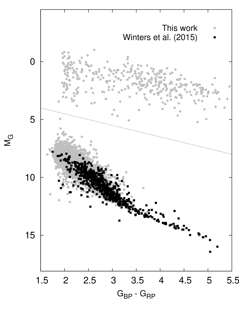
Figure 2: Top: Colour-absolute magnitude diagram of about 1.4 million M stars with Gaia colours and parallax (symbols as in Fig. 1): the dashed line clearly separates dwarfs from giants. Bottom: Box and Whisker plot showing minimum, 1st quartile, median, 3rd quartile and maximum distances of M dwarfs for each colour bin. Note the hard cutoff at 1.5 kpc distance in our selection.

We select our sample of M-dwarfs in three steps: first we consider the SkyMapper properties of known M-dwarfs to inform our search box; then we apply corresponding colour criteria to the full SkyMapper DR1 to create a sample of M stars; and finally we use astrometric measurements from the second data release (DR2; Gaia Collaboration et al., 2018a) of ESA’s Gaia mission (Gaia Collaboration et al., 2016) to separate dwarfs from giants.

Our starting point is the recent compilation of Southern M dwarfs within 25pc from the Sun by Winters et al. (2015). While this catalogue does not contain all known M dwarfs in the Southern hemisphere (Dec $\leq$ 0^∘), it does include 1748 genuine M-dwarfs ranging from spectral type M0V to M9.5V. We cross-match this volume-limited sample with the SkyMapper master table of the release version DR1.1 while taking into account proper motion: we find SkyMapper matches for $\sim 97$% of the sources, whereas the remaining 3% are missed due to incomplete sky coverage in DR1. When comparing positions with external catalogues, we simply use the mid-time of the observations, mid-October 2014, as the reference epoch for DR1 sources.

Next, we apply the following data quality cuts:

• FLAGS<4: the flags are a combination of Source Extractor flags and bespoke quality flags from the SkyMapper Science Data Pipeline (SDP; for details see Wolf et al., 2018) that warn against unreliable photometry.

• prox>5: a proximity criterion that requires the nearest neighbour source to be at least 5 arcsec away as we don’t trust the photometry otherwise.

• nch_max=1: this means that the source is not detected as a blend of multiple sources.

• ebmv_sfd<0.2: moderate interstellar reddening as described by the maps of Schlegel et al. (1998).

• {F}_nvisit$\geq$2: requires two or more visits in each filter {F} (with {F} in {$uvgriz$}), to include the source in the list.

We do not deredden the photometry of these nearby M dwarfs as their distance places them inside the dust-poor local bubble, which extends more than 50 pc in all directions (Frisch et al., 2011). The sample forms a well-defined locus in the $riz$ diagram which meets the following criteria:

$$0.75<r-i<3.5~{},~{}0.25<i-z<1.7~{},~{}r<18~{}.$$ (1)

It is not necessary to consider $uvg$ colour cuts because these red objects, even at close distance, tend to be very faint in those bands.

Next, we select a sample of M-star candidates with the same criteria from the overall DR1 catalogue. Here, we correct the observed colours for reddening using the reddening coefficients listed by Wolf et al. (2018). We obtain a flux-limited sample of 1 504 379 objects covering nearly the full Southern hemisphere except for the higher-reddening zone at low Galactic latitudes. Fig. 1 shows our selection region in the $riz$ colour-colour diagram and contains both our candidate sample and the known M dwarfs (black points) from Winters et al. (2015).

As a last step, we remove M giants from our sample, which are indistinguishable with only $riz$ colours. Hence, we restrict the sample to sources with a full five-parameter astrometric solution (position, proper motions and parallax) from Gaia DR2 to make a colour-absolute magnitude diagram (CaMD). DR1.1 has been pre-matched to Gaia DR2 and the SkyMapper data portal contains a copy of the Gaia catalogue as a separate table ext.gaia_dr2. However, this pre-match does not take proper motion into account, and hence we redo the match with proper motion folded in. Sometimes, we find ambiguous matches to more than one Gaia object, and we choose to clean the sample simply by dropping those stars where the Gaia magnitude indicates a star of the wrong brightness. We thus ensure that we get a clean sample for reliable distance estimates. We also avoid the risk of the SkyMapper magnitude being compromised by blended sources when Gaia offers more than one possible counterpart.

A simple parallax inversion gives a poor distance estimation in the presence of non-negligible errors on the parallax $\varpi$ (see Luri et al. 2018; Bailer-Jones 2015 for a detailed discussion). Instead, we adopt the Bayesian approach proposed by Astraatmadja & Bailer-Jones (2016) to infer the most probable distance, in which we use a prior that varies with distance according to an exponentially decreasing space density distribution (with a length scale $L$ = 1 kpc). We then remove all objects that would be further than 1.5 kpc to restrict our analysis to disc stars in the solar neighbourhood. For the majority of these sources, the relative precision on $\varpi$ is better than 20%, which means that we would also be able to simply estimate the absolute Gaia magnitude using the distance modulus equation (e.g., Gaia Collaboration et al. 2018b).

Fig. 2 shows a clear separation between dwarfs and giants on the CaMD. We choose to remove M giants (some of which could turn out to be long-period variables, e.g. Mowlavi et al., 2018) by placing a final cut in luminosity within the gap, using $M_{G}<2.5+(G_{BP}-G_{RP})$. At this point, our sample includes 1,386,114 objects with 4,361,814 observation blocks. In our flux-limited sample, early- to mid-type M dwarfs ($G_{\mathrm{BP}}-G_{\mathrm{RP}}\leq 3.5$) can be seen out to distances of 1.5 kpc, while later types cover smaller volumes (see bottom panel in Fig. 2). Note, that we do not de-redden $G_{\mathrm{BP}}-G_{\mathrm{RP}}$ colours because we do not have 3D extinction maps, but we checked how large the influence might be, but the most extreme cases in our sample are distant M0 dwarfs along specific lines-of-sight at low $b$. There, we find a colour correction of $E(G_{\mathrm{BP}}-G_{\mathrm{RP}})\la 0.25$ mag, which is small relative to the full colour range of 4 mag. We checked that the result figures would not change significantly.

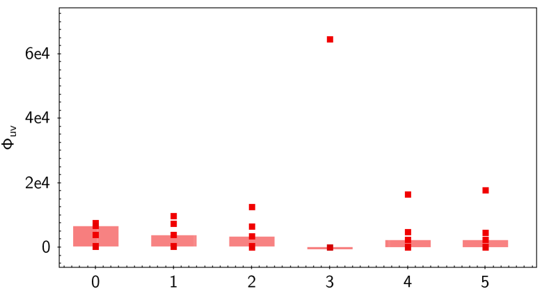
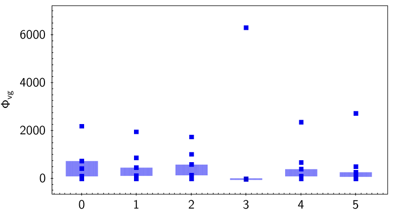
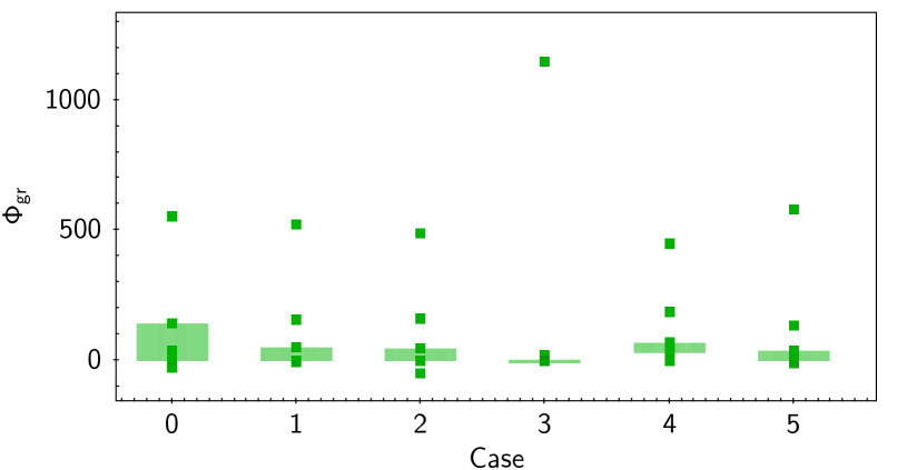
Figure 3: Schematic diagram of the leave-one-out cross-validation algorithm to estimate the quiescent magnitudes of M dwarfs. The full light curve of this example object consists of five observation blocks that are indicated by a label on the x-axis (from Case 1 to Case 5). Case 0 shows an initial guess of ${\Phi}_{ij}$ values using all data points, while in the other cases $\hat{\Phi}_{ij,n}$ statistics are calculated by dropping the data points for epoch $n$. The shaded bars represent the $1\sigma$ RMS scatter of the flare variability indices.

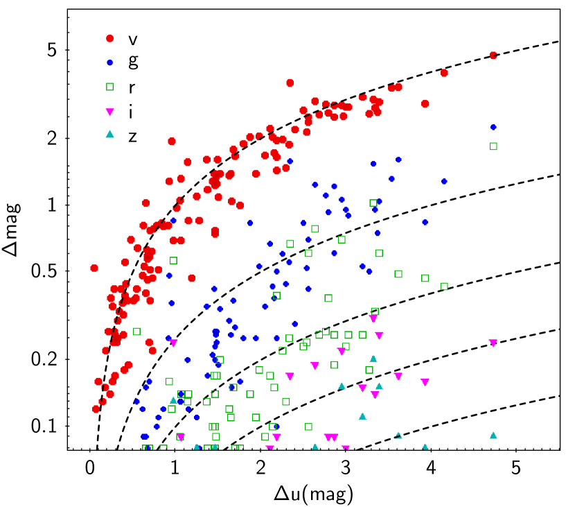
Figure 4: Relation between the $u$ band amplitude and the near-simultaneous multi-colour ($vgriz$) amplitudes for 129 M-dwarf flares detected with $\Phi_{uv}$. Dashed lines indicate amplitudes relative to the $u$ band, from top to bottom: 100%, 25%, 10%, 5%, and 2.5%, respectively.

3 Correlation-based flare detection: dm-dt-filter pairs

We identify flare candidate events using a flare variability index $\Phi$ formed from filter pairs in each observation block $n$. This method was also used by previous flare searches (e.g. Kowalski et al., 2009; Davenport et al., 2012)). The flare variability index can be written in general form as

$$\Phi_{ij,n}=[\frac{m_{i,n}-\overline{m}_{i}}{\sigma_{i,n}}][\frac{m_{j,n}-\overline{m}_{j}}{\sigma_{j,n}}]~{},$$ (2)

where $i$ and $j$ denote two different filters, e.g., $uv$, $vg$, or $iz$. While $\overline{m}_{i,j}$ are the quiescent magnitudes of those filters, $m_{i,j}$ are single measurement points (mag_psf) for each filter at epoch $n$, and $\sigma_{i,j}$ are their errors (e_mag_psf).

The main difficulty in searching for flaring epochs is to properly estimate the quiescent flux level, which is a bit challenging as most sources in DR1 have less than five observation blocks. In sources where we observe a flare, the mean magnitudes do not represent the quiescent level but an average biased by the flare itself. Thus, we estimate the quiescent flux level by examining the light curve with a rolling leave-one-out strategy that removes possible flare epochs. To avoid artefacts, we only consider photometric measurements that have no bad pixels contained in an object’s aperture, as indicated by nimaflags=0. Our search for flare candidates loops over all objects in the M dwarf parent sample and considers each possible flare epoch $n$ separately; leaving out epoch $n$, we estimate the quiescent flux level and the $\hat{\Phi}$ statistic:

$$\hat{\Phi}_{ij,n}=[\frac{m_{i,n}-\overline{m}_{i,n}}{\sigma_{i,n}}][\frac{m_{j,n}-\overline{m}_{j,n}}{\sigma_{j,n}}]~{},$$ (3)

where $\overline{m}_{i,n}$ and $\overline{m}_{j,n}$ are the weighted means obtained by dropping the measurements for epoch $n$. In a noisy case without outliers, the flare variability index is close to a normal distribution with a mean of $\hat{\Phi}_{ij}\approx 0$. In a flaring star, the root-mean-square of the leftover measurements will shrink dramatically, when the flaring epoch is left out, clearly marking the epoch to be left out. We thus simultaneously get unbiased estimates of the quiescent magnitude and the flare variability index.

When flares are weak and close to the noise level, we can still detect them as to be left out by combining the answer from all six passbands. Our observing sequence creates a strong correlation among the six measured magnitudes for the same epoch $n$.

Fig. 3 shows an example of the $\hat{\Phi}$ statistic from a flaring M dwarf: the initial quiescence level of $\hat{\Phi}$ in this star is overestimated due to the outlying flare measurements in the third observation block. This effect is largest in the bluest bands, where the flare emission shows the highest contrast over the quiescent flux (e.g. Bochanski et al., 2007; Kowalski et al., 2013).

Now we select flare candidates by looking for brightening in adjacent filters occurring nearly simultaneously within observation blocks. We require: $m_{i,n}-\overline{m}_{i}<0$ AND $m_{j,n}-\overline{m}_{j}<0$ AND $\Phi_{ij}$ > 0. However, candidate signals can also be produced by correlated random noise in our light curves. Miller et al. (2001) describe the false discovery rate (FDR) approach as one way to control the number of false positives. By comparing the flare candidate distribution ($\Phi_{ij}$ > 0; test hypothesis) with an underlying noise distribution caused by random photometric errors ($\Phi_{ij}$ < 0; null hypothesis), we can set a threshold value tuned to a desired low level of false positives for each filter pair separately. We determine the probability distribution function for each null-hypothesis estimator, which is well approximated by a normal distribution, by calculating the $p$-values for the test distribution. By setting the FDR parameter to $\alpha=0.05$, we ensure that our flare sample ends up with a contamination fraction of only 5%. This fraction corresponds to threshold values of 540, 420, 880, 755, 765 for $\Phi_{uv}$, $\Phi_{vg}$, $\Phi_{gr}$, $\Phi_{ri}$, $\Phi_{iz}$, respectively.

Figure 5: Flare amplitude vs. flare variability index in the most (top) and least (bottom) sensitive filter pairs. The background colour maps show the number density of objects. Towards the top right, we see flares, whether they are unique (solid symbols) or duplicate (open symbols). Duplicates are flares detected in more than one filter pair.

Table 2: Summary of flare candidates from SkyMapper DR1

		Number of flare epochs
$\Phi_{ij}$	Number of observed epochs	$\Phi_{ij}>0$	$\alpha\simeq 0.05$	SNR $\geq 3.0$	Eyeball	Unique	Duplicate
$\Phi_{uv}$	46,758	9,362	200	162	129	129	-
$\Phi_{vg}$	63,711	13,881	146	131	101	27	74
$\Phi_{gr}$	2,398,357	566,859	154	130	105	48	57
$\Phi_{ri}$	3,834,884	924,550	196	143	81	41	40
$\Phi_{iz}$	4,075,290	1,015,531	171	118	29	9	20
Total	10,419,000	2,530,183	867	684	445	254	191

Next, we clean the candidate sample further by removing events that are too weak to provide conclusive evidence for bona-fide flares. Fig. 4 gives an empirical relation between $u$ band and $vgriz$ band amplitudes of flare candidates selected by the $\Phi_{uv}$ index. As expected, there is a one-to-one correlation between $\Delta u$ and $\Delta v$ but the resulting $\Delta m_{i}(=|m_{i,n}-\overline{m}_{i}|$) for the $griz$ bands are an order of magnitude lower than the $uv$ bands, even in large-amplitude flares of $\Delta u,v>1$ mag. This wavelength-dependent variability is an ubiquitous characteristic of M-dwarf flares and reproduced by a semi-analytic two-component flare model (Davenport et al., 2012). Thus, our efficiency of recovering low-amplitude flares is limited by the light curve root-mean-square ($\sigma_{LC,i}$) scatter as a function of source magnitude. In the case of the $uv$-filter pairs, where enhanced blue continuum is significant during flares, the trade-off is an increase in the noise level due to the faint nature of M dwarfs in blue optical bands. The flare variability is measured with a signal-to-noise ratio given by SNR = $\Delta m_{i}/\sigma_{LC,i}$. To construct a fairly complete sample of flares, we apply the same SNR threshold of 3.0 to all filter pairs. This implies the error on our measurement of the amplitude of variability can be up to $\sim$33%. Fig. 5 shows the relation between flare variability index and flare amplitude in the most and least sensitive filter pairs. Plausible candidates are found in the outlying low-density regions. Some events in those regions are not marked as candidates, but these are cases where the magnitude decreases in both bands simultaneously ($m_{i,n}-\overline{m}_{i}>0$ AND $m_{j,n}-\overline{m}_{j}>0$ AND $\Phi_{ij}$ > 0), so these are possible eclipse-like events if they are significant.

Finally, we eyeball the multi-colour light curves of all candidate events and remove unreliable light curves, whose (i) overall variability does not follow the pattern of a typical flare variation in all six bands (i.e. a rapid rise that decreases with wavelength) or (ii) variability signal is still dominated by systematic errors (i.e. the observed changes in magnitude were comparable to the uncertainties for some filter pairs).

4 Results and Discussion

Using our conservative detection thresholds for searching dm-dt-filter parameter space, we find 445 flare signals from 254 unique stars among 10,419,000 observed epochs in any filter combinations (summarised in Table 2). Ten of our flaring stars are listed in the AAVSO International Variable Star Index (VSX; Watson et al., 2006, 2017), which is cross-matched to DR1 in table ext.vsx. They are classified as eruptive stars (INS and UV), spotted stars (ROT), and active binary systems (RS and EA).

We also use the SkyBoT cone-search service (Berthier et al., 2006) to check the list of available solar system objects (e.g., asteroids, planets and comets) located in our field-of-view at all given epochs. We find no flare events that were cross-matched with the position of any known moving objects.

4.1 Large-amplitude flares: $\Delta m>1$ mag

Flares with amplitudes larger than 1 mag can be found most easily at the blue end of the spectrum due to the higher contrast. In $u$- and $v$ band we find 69 and 79 large-amplitude flares, respectively, which combine to 92 unique flares in total. The numbers rapidly decline towards redder passbands, with 17 and 2 flares in $g$- and $r$ band, respectively.

Even the largest $uv$ flares in our sample show a flux enhancement of only 0.1 to 0.3 mag in our reddest $iz$ filters, where we find not a single large-amplitude flare. This already implies that potential searches for extragalactic transients will have to deal with much less foreground fog if done in the $iz$ bands. However, in Section 4.4 we discuss events outside our flare sample, which appear extreme enough to cause large-amplitude changes in the $iz$ bands.

Our ability to discover extremely bright flares is limited by the rejection of saturated measurements from the parent data set. The filters reaching the most shallow magnitudes are $u$ and $v$, with an average saturation limit of 9 mag. Most stars are at the faint end with quiescent magnitudes of $u=16\ldots 18$, where saturation limits us to flares of $\Delta u<7\ldots 9$. This implies that we are largely sensitive to much more extreme flares than the brightest single event in our sample, which has $\Delta u\approx 4.7$ (see Fig. 4). Also, the single brightest star in our sample has $u\approx 14$ and $v\approx 14$, which limits the dynamic range for flare detection to $\Delta u<5$. We thus consider it unlikely that we have missed an extreme flare due to saturation.

4.2 Flare spectral energy distribution from SkyMapper uvgriz photometry

Spectral energy distributions (SEDs) of flares provide important constraints for their physical models, their simulation and radiation mechanisms. In the past, M dwarf flares have mostly been observed in Johnson $U$ band (3300–4000Å) where they show the highest contrast within the spectral range of CCDs. Some observations of flares cover the full range of $UBVR$ bands and suggests that flares around peak resemble a featureless, blackbody-like emission with temperatures of $T\sim$9 000–10 000 K (e.g. Hawley & Fisher, 1992; Hawley et al., 2003; Kowalski et al., 2013). However, it is difficult to disentangle the relative contributions from higher-order Balmer lines in broadband filters (Allred et al., 2006; Kowalski et al., 2019). Here, the SkyMapper filters might have an advantage as they split the $U$ band into two, the ultraviolet $u$ band (centre: 349nm/width: 42nm) and the violet $v$ band (384nm/28nm). In the following, we will investigate this possibility.

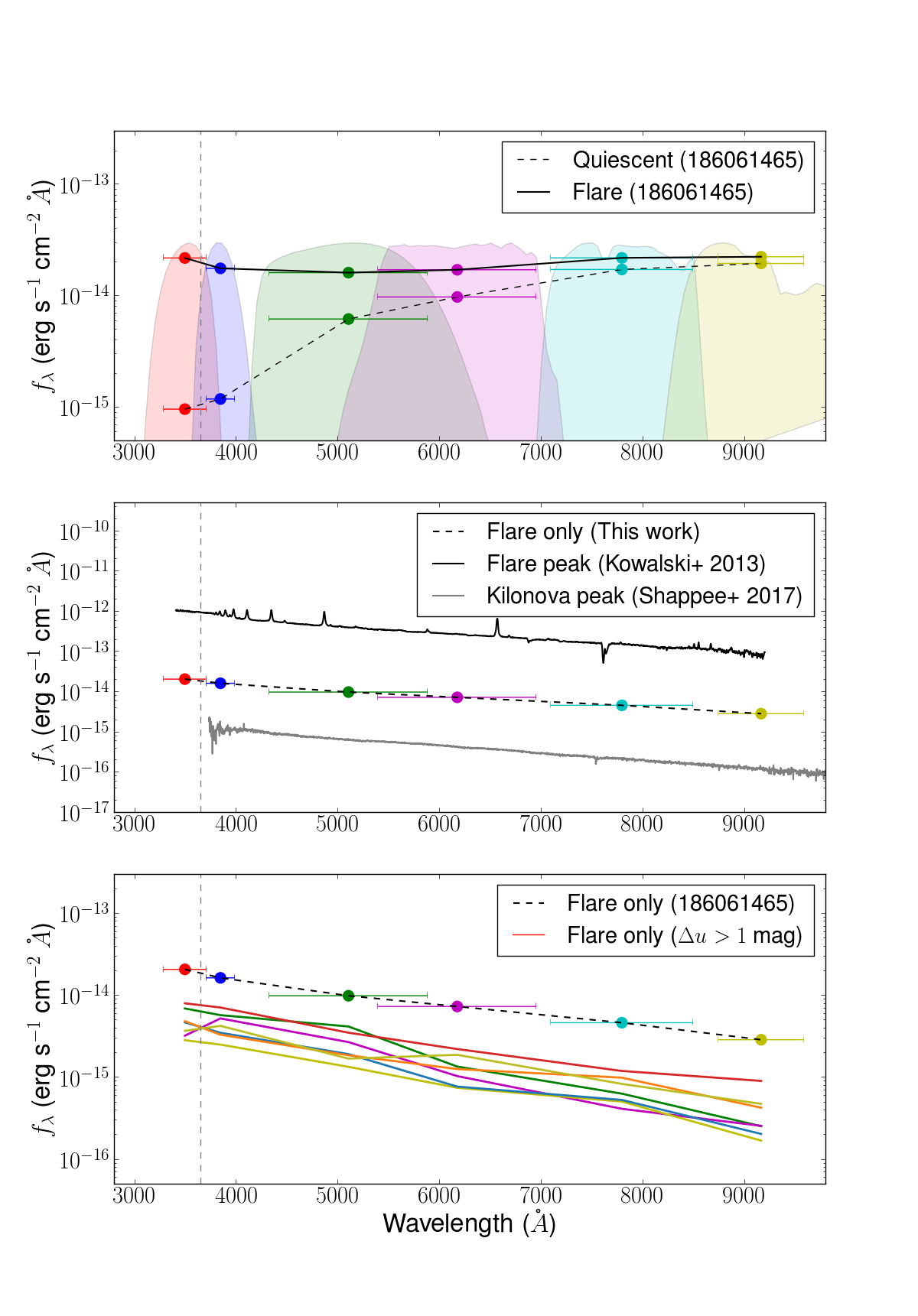
Figure 6: Top: spectral energy distribution of an M dwarf (DR1 object_id = 186061465; SMSS J134839.68-452710.2) during a large flare with $\Delta u=3.4$ (solid line) and in quiescence (dashed line). The vertical line marks the Balmer jump at 3646Å. Normalised transmission curves for SkyMapper $uvgriz$ filter are shown as lighter shaded regions. Middle: The flare SED after subtracting the quiescent flux, compared with the spectrum of YZ CMi at flare peak (black line; Kowalski et al. 2013) and the 0.49-day spectrum of the kilonova from GW170817 (grey line; Shappee et al. 2017). Bottom: The flare-only SEDs for M dwarf flares with large amplitude ($\Delta u>1.0$ mag) in our sample.

To obtain flux densities $F_{\lambda}$ in each of the SkyMapper filters during the quiescent and flare states, we convert SkyMapper AB magnitudes into flux densities $f_{\lambda}$ following the definition of Bessell & Murphy (2012). Fig. 6 compares the SED of one M dwarf in the non-flaring and flaring state. The former shows a normal M dwarf SED with $T_{\mathrm{eff}}$ $\simeq$ 3500 K, while the blue upturn in the latter is a clear sign of a composite spectrum. After subtracting the SED in the quiescent state, we compare the flare-only SED with a peak-phase spectrum of a flare on the M dwarf YZ CMi (Kowalski et al., 2013), and with the earliest spectrum of a kilonova observed $\sim$12 hours after a binary neutron-star merger (Shappee et al., 2017). All three appear to be characterised by black-body emission with similar temperatures of $\sim$10,000 K. In the bottom panel of Fig. 6, we show the flare-only SEDs of flares with large amplitude variations of $\Delta u>1$ mag. These large amplitude flares are likely observed near the peak epoch because all the flare-only SEDs are dominated by hot black-body emission with a temperatures of $\sim$10 000 K. It is also trivially expected that flares seen near peak will show up preferentially with larger amplitudes.

To investigate the flare temperature and mix of radiation mechanisms in detail, we check colour-colour diagrams of flares with large amplitudes ($\Delta u\geq 1$ mag) that could be close to flare peak. Our measurements of these events are all blue and centred on $(u-v)_{0}\approx 0$ and $(v-g)_{0}\approx 0$, indicative of black-body temperatures between 10 000 K and 20 000 K. But there is significant scatter around this mean colour, which is caused in part by the short time difference between observations of the $uvg$ filters, during which the flare evolves in brightness. More importantly, it might be caused by the Balmer continuum with a wide range of relative contributions to the continuum flux in the $uv$ filters. Thus, we cannot determine the exact flare temperature only by colour information without simultaneous spectra.

4.3 Flaring fraction of M dwarfs by type and position

The nearly complete coverage of a whole hemisphere of sky allows us to investigate with high statistical significance the flaring fraction of nearby M dwarfs as a function of spectral subtype and position in the Galaxy. The observed flare volume is unbiased within the considered area (2 965 SkyMapper fields with $\sim$16 900 deg²), which covers a wide range in Galactic longitudes ($0\degr$ to $360\degr$) and latitudes ($-90\degr$ to $-10\degr$ and $+10\degr$ to $+70\degr$). We avoid higher-reddening regions as these are coincident with crowded regions, where it is difficult to measure accurate photometry. In this section, we will derive robust statistics of flare rates by grouping stars by their properties with at least 1 000 stars per bin and measuring the flare fraction from our flare sample.

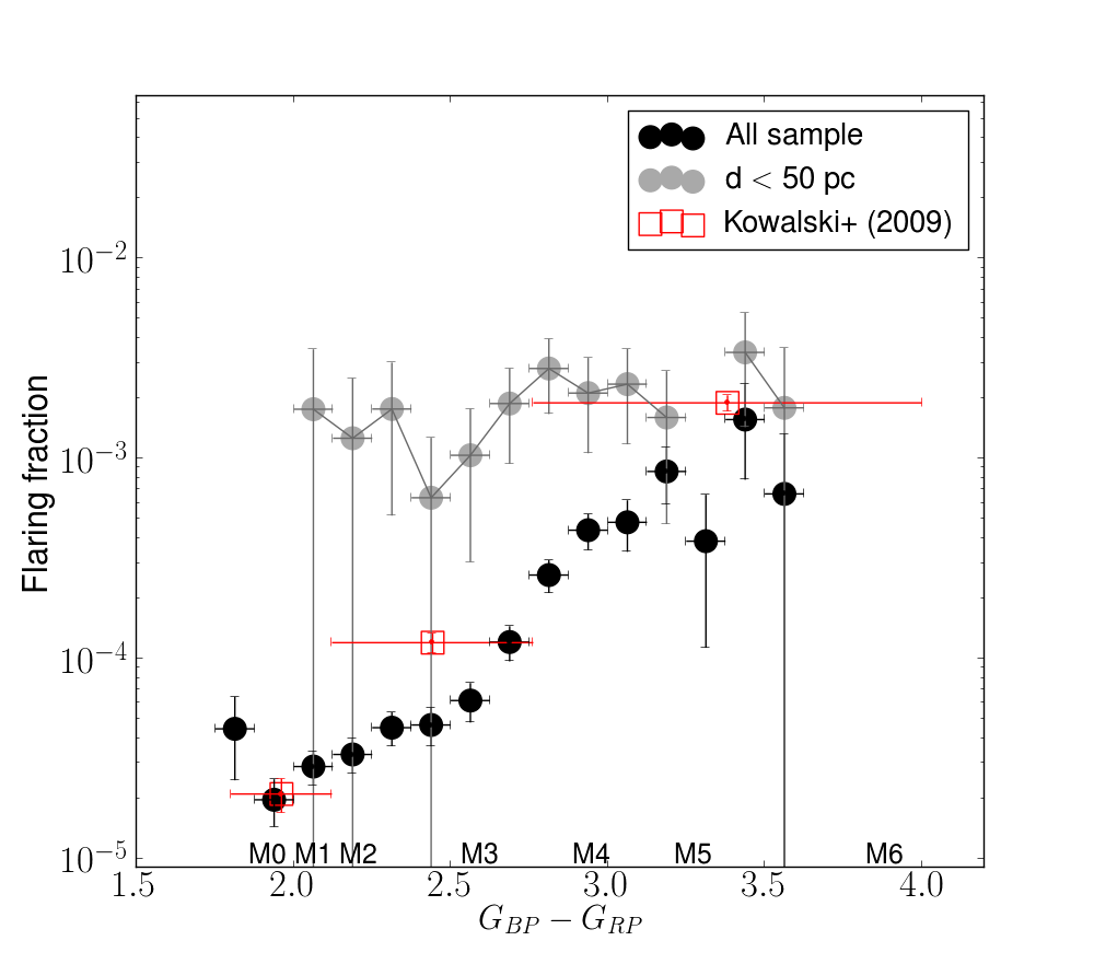
Figure 7: Flaring fraction vs. colour: horizontal error bars are bin width and vertical errors bars are Poisson uncertainties. Spectral types mark the colours of Pickles (1998) dwarf templates. The Kowalski et al. (2009) points (open squares) have been placed to match the spectral types and are consistent with our full flare sample (black symbols). Grey symbols show a volume-limited sample within 50 pc distance from the Sun.

We investigate the fraction of M dwarfs that flare as a function of Gaia colour ($G_{\mathrm{BP}}-G_{\mathrm{RP}}$) in bins of 0.125 mag. The flare fraction is defined as the ratio between the number of flare epochs and the total number of observed M dwarf epochs (flaring or not), or in other words, the fraction of stars seen as flaring in an instantaneous snapshot of the sky. This is shown in Fig. 7, where we see a clear trend of increasing flaring fraction towards redder colour in the black points that represent the whole sample. The flaring fraction rises from $\sim 30$ flares per million stars for early M dwarfs ($G_{\mathrm{BP}}-G_{\mathrm{RP}}$ $\sim 2$) to $\sim$1 000 flares per million stars for late M dwarfs ($G_{\mathrm{BP}}-G_{\mathrm{RP}}$ $\sim 3.5$). We place sub-type labels in Fig. 7 based on synthetic photometry of the Pickles (1998) templates.

We compare this result to a flare sample of nearly equal size (Kowalski et al., 2009) that was obtained in the much smaller-area SDSS Stripe 82 from repeat observations over roughly 60 epochs. This latter sample covers about 280 deg² along the celestial equator stretching in Galactic longitude across $45\degr<l<191\degr$ and in latitude across $-64\degr<b<-21\degr$. Our distribution is similar to theirs, but provides tighter constraints for the flaring fraction as a function of colour.

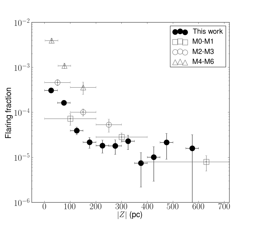
Figure 8: Fraction of flaring epochs as a function of vertical distance, $|Z|$, from the galactic plane (black points, $|Z|$ bin size 50 pc). Error bars are Poisson uncertainties in the flaring fraction and bin width in $|Z|$. We overlay results from Kowalski et al. (2009) for their spectral type ranges (M0–M1: open squares, M2–M3: open circles and M4–M6: open triangles).

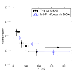
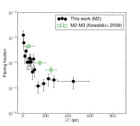
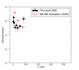
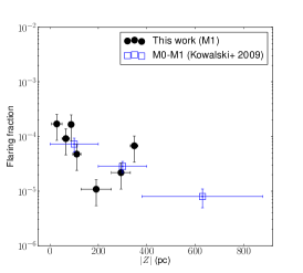
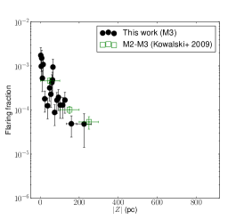
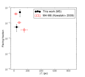
Figure 9: Same as Fig. 8 but showing the results for spectral subtypes from M0 (top left) to M5 (bottom right). The width of the $|Z|$ bins is adjusted so that they include a constant number of flare events.

One interesting feature in our distribution is that the flaring fraction appears to increase steeply between M3 and M4 spectral type. Perhaps by coincidence, this is also the regime where the interior structure of main-sequence dwarf stars is thought to transition from partially to fully convective and where an abrupt change in the large-scale magnetic topology is expected (see Stassun et al. 2011 and references therein). Also, Rabus et al. (2019) identified a sharp transition region in the $T_{\mathrm{eff}}$–radius plane between partially and fully convective M-dwarfs, which appears at a magnitude $M_{\mathrm{G}}\sim$11–11.5 and a colour of $G_{\mathrm{BP}}-G_{\mathrm{RP}}$ = 2.55–3.0 (see fig. 9 of Rabus et al. 2019). For these reasons, the feature in the trend may appear to be physically meaningful.

However, this is also the colour range where our search volume changes from including the thick disc and halo to only the thin disc, so that the age distribution of our stars changes rapidly across the M3-to-M4 range. For this reason, we also consider the flare fraction in a smaller sample limited to a small vertical distance from the plane of the Galaxy of $|Z|<50$ pc, where we expect little age gradient within the volume. But in that sample we find at low Galactic latitude that we reach large distances for the stars, but only closer distances for the detected flares, so that the sensitivity of flare detection is still correlated with spectral type.

Then we consider a volume-limited sample of stars and flares within a solar neighbourhood of $d<50$ pc, which is not only expected to be free of age gradients but also statistically more complete in its flare detection. This sample includes 5 889 stars with 18 979 observation blocks and 32 flares. The results of the volume-limited sample are shown as grey points in Fig. 7 and surprisingly show no dependence on spectral subtype – instead we find a constant flaring fraction of $\sim$1 650 per million M stars across the types from M1 to M5. Given that our flare detection is mostly limited by changes in $u$ band magnitude, this finding suggests that flare rates are constant when selecting flares by power relative to $u$ band luminosity of the star, i.e. we find qualitatively that “strong flares on bright stars are as common as weak flares on faint stars”. Going towards warmer stars, we still expect the flare rate to drop eventually, but we don’t see the turnover in the range of M dwarfs.

We also investigate the flaring fraction as a function of the vertical distance $|Z|$ from the Galactic plane and thus as a function of stellar age. Following Gaia Collaboration et al. (2018c), we compute the Galactic cylindrical coordinates ($R,\phi,Z$) where the radial distance of the Sun from the Galactic centre is assumed as $R_{\odot}=8.34$ kpc and the height of the Sun above the plane is $Z_{\odot}=27$ pc. As in the SDSS flare sample, the range of vertical distance in the sample varies with the observed brightness of the stars. In our sample, early M dwarfs ($G_{\mathrm{BP}}-G_{\mathrm{RP}}$ = 2) are visible up to $|Z|=1.5$ kpc, while late M dwarfs ($G_{\mathrm{BP}}-G_{\mathrm{RP}}$ = 3.5) are confined to within $|Z|=200$ pc. Fig. 8 shows a strong dependence of the flaring fraction on $|Z|$, similar to the trends seen in earlier photometric and spectroscopic samples (e.g., Kowalski et al. 2009; Hilton et al. 2010; West et al. 2011). Since the slope of this relation varies as a function of spectral type, we show the SDSS results for three different spectral ranges. Note that distances to the SDSS stars were determined with a photometric parallax relation and are thus less certain and not necessarily consistent with our distance scale derived from Gaia. The mean flaring fraction in our combined sample is consistent with early M dwarfs (M0-M1) in Stripe 82, and these are the dominant objects in our flux-limited sample. We also find that M dwarfs within 150 pc of the Galactic plane show relatively larger flaring fraction than those farther from the plane, which seem to converge towards a level of 10 to 20 per million. This decline is usually explained by a rapidly declining magnetic activity in older stars (West et al., 2006, 2008), which were born in the Galactic disc a long time ago, but were dynamically heated by gravitational interaction and scattered into orbits with larger mean $|Z|$.

Lastly, we check the results on the $|Z|$ dependence by spectral subtype to see if the trend is an artefact of mixing spectral types. In Fig. 9 we show the dependence on $|Z|$ for six subtypes in our sample, from M0 to M5. We choose the bin width in $|Z|$ such that we have the same number of flares in each bin. Where we have sensitivity, we see that the flaring fraction closest to the plane of the Milky Way is over 1 000 per million stars, while at more than 150 pc vertical distance it has dropped to a few tens per million stars and tends to stay flat beyond. These trends are fairly similar across the subtypes from M0 to M3 at least.

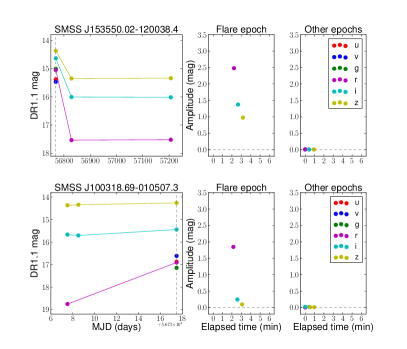
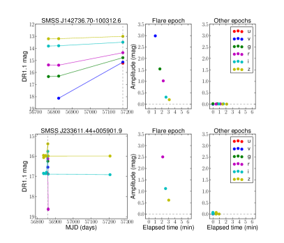
Figure 10: Light curves of four high-amplitude flares with large continuum enhancement in the redder filters. The panels to the right show a zoom-in of the flaring epoch and a non-flaring epoch for comparison. The objects are labelled with their SMSS object IDs.

Table 3: Flaring fraction for M dwarfs observed in different ranges of Galactic latitude.

Galactic latitude	Number of stars	All observed blocks	Flaring blocks	Flaring fraction $f$ per million stars
$10\degr\leq|b|<15\degr$	90,996	261,651	24	$91.7\pm 18.7$
$15\degr\leq|b|<30\degr$	423,294	1,281,113	78	$60.9\pm 6.9$
$30\degr\leq|b|<45\degr$	385,349	1,217,773	66	$54.2\pm 6.7$
$45\degr\leq|b|<60\degr$	281,214	936,723	50	$53.4\pm 7.5$
$60\degr\leq|b|<75\degr$	162,632	536,516	31	$57.8\pm 10.4$
$75\degr\leq|b|<90\degr$	42,629	128,038	5	$39.1\pm 17.5$
Total ($15\degr\leq|b|<90\degr$)	1,295,118	4,100,163	230	$56.1\pm 3.7$
Total ($10\degr\leq|b|<90\degr$)	1,386,114	4,361,814	254	$58.2\pm 3.6$

4.4 Extreme flare candidates in red passbands

We investigate extreme flare cases in the master table, where the quiescent star is not visible in the $uvg$ bands. We define this subsample as one where we detect only the flare epoch in the bluer filters ({F}_ngood=1), while the $r$ band detections are marginal (r_ngood=2) and the $iz$ detections are regular ({F}_ngood>2) to get reliable magnitudes in quiescence for applying at least the colour cut $0.25<i-z<1.7$. We find 134 objects that are not included in our main analysis, three of which appeared to show flares according to our selection criteria. These three objects show exceptionally large variations of $\Delta m>1$ mag in the $i$ band, but two of them were identified as Mira-type stars later with VSX matches.

The only plausible extreme flare is an $i$ band flare with $\Delta i$=1.1 mag from the M dwarf SMSS J233611.44+005901.9 with estimated flare magnitudes of $>$5.1, $>$5.1, 3.4, 2.5, 0.6 mag for the $uvgrz$ bands, respectively. Fig. 10 shows this flare alongside three weaker ones. Now, that DR2 of SkyMapper is available (Onken et al., 2019) and includes deeper images one third of the Southern sky, we can obtain more precise colour indices of this object in quiescence, $(r-i,i-z)=(2.295,0.917)$, which indicate a spectral type of M4–M5 that lies on the locus of typical M dwarf stars (see Fig. 1). For comparison, following the method outlined in Davenport et al. (2012), we simulate a 1.1 mag $i$ band flare on an M4 star and thus predict amplitudes in the SDSS $ugriz$ filters of (6.9, 3.7, 2.2, 1.1, 0.6 mag), to which our observed flare amplitudes are well matched. The shape of the SED is perfectly consistent with an M dwarf flare, making it unlikely that this transient is caused by a blend with an unknown asteroid.

In Fig. 10, we highlight the light curves of rare, high-amplitude flares, which have either $r$ or $i$ amplitudes of $\geq$ 1 mag. Only one of them, SMSS J100318.69-010507.3, has a Simbad spectral classification (M7Ve) with a strong H_α emission (Gizis, 2002), further supporting evidence of a young, active star (see bottom left panel of Fig. 10). As expected, extreme flares are very rare in the $iz$ filters, with a flaring fraction of $\sim 0.5$ per million stars.

5 The foreground fog and searches for rare events

M-dwarf flares are the dominant source of transients in time-domain surveys. We now explore how they might contaminate searches for rare extragalactic transients. A particular scenario is large-area searches for optical counterparts to gravitational-wave (GW) events detected by the LIGO/Virgo facilities (Abbott et al., 2017; Andreoni et al., 2017), with the aim of identifying potential kilonova emission as early after the GW event as possible. Typical cases may involve searching an area of 100 square degrees.

To estimate the predicted rate of M dwarf flares for the kilonova search by SkyMapper, we first calculate the mean observed fraction of M dwarf flares above our detection limits as a function of Galactic latitude $|b|$. Table 3 shows that the flaring fraction $f$ is mostly constant, except for low latitudes, where the mean age and the mean flare rate of thin-disc M dwarfs suddenly changes. The highest-latitude bin appears to show a lower fraction, but given its larger error bar this is insignificant. Overall, we find a flaring fraction of $\sim 56$ per million stars at $|b|>15$, while close to the plane this fraction might increase.

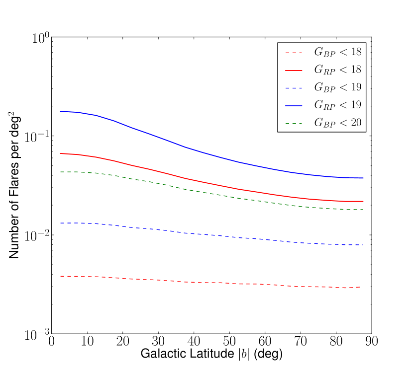
Figure 11: Surface density of M dwarf flares with $\Delta u>0.1$ mag for samples of different depth in Gaia passbands.

We now use the most up-to-date simulation of the Gaia Universe Model Snapshot (GUMS-18: Robin et al. 2012) to select M dwarfs above a given detection limit and to estimate how many flares a time-domain survey will see instantaneously. This simulation contains about 2.1 billion objects uniformly distributed in the sky that can be observed by Gaia, down to a limiting magnitude of $G=20$. We extract all M dwarfs ranging from spectral type M0V to M9V based on the Gaia Object Generator (GOG18: Luri et al. 2014) catalogue, which is the transformation of GUMS-18 into Gaia final catalogue data. We divide the total M dwarf sample into three subsamples covering different magnitude cuts (18, 19 and 20th mag) in each Gaia band. The cumulative number of M dwarfs in the red band, N ($<G_{\mathrm{RP}}$ = 18–19, which includes 32–76M detectable objects), is an order of magnitude larger than that in the blue band (2–8M objects). We drop the case of $G_{RP}<20$ because the red sample is incomplete at $G_{RP}>19$.

According to the Gaia simulation, the number density of $G_{RP}$ band M dwarfs is decreasing with increasing latitude $|b|$, ranging from a few thousand to a few hundred objects per square degrees. We multiply the number density with the flaring fraction derived by this work to obtain an instantaneous rate of flares that would be found in a single visit. Fig. 11 shows the expected number of flares from M dwarfs brighter than a given Gaia magnitude limit per square degrees as a function of galactic latitude. Due to the assumed flat slope of our observed flaring fraction with galactic latitude, the overall distribution is primarily driven by number density rather than physical changes. Although the flare rate of M dwarfs has a strong dependence on spectral type and age, our results are still strongly dominated by the number density of M dwarfs for each spectral type. In the Gaia simulation, more than 80 and 16 percent of the objects in the sample are early-type (M0-M1) and mid-type M dwarfs (M2-M3), respectively. The number of late-type M dwarfs (M4-M5) is more than two orders of magnitude below the dominant sample. We can compute the expected number of flares from M dwarfs that would be seen down to a given Gaia magnitude during a hypothetical snapshot observation that covers 100 square degrees (Table 4). Over this area we expect to observe about one flare with $\Delta u>0.1$ mag from M dwarfs with $G_{\mathrm{BP}}<19$, whereas we expect 4 to 18 flares from M dwarfs with $G_{\mathrm{RP}}<19$, depending on the line of sight through the Galaxy.

How many flares will be seen by a survey within a given magnitude limit depends on the flare contrast and thus on the observed passband. While there are many more M stars seen in quiescence in redder bands, the relative amplitude of flares is much smaller than in blue passbands. Given the flare temperature, flaring stars can appear brighter in the blue than in the red during the rare extreme flares. Therefore, a prediction of expected flares in observations with blue passbands would need to consider much fainter M dwarfs than considered in the Gaia simulation. This means that searches for transients in the blue will be dominated by flares that appear to come out of nowhere, as blue images will not show the stars they originate from in quiescence. While a detailed interpretation of this contamination as a function of apparent peak magnitude of the flare is beyond the scope of this work, we do note, that knowing about the presence of an M dwarf at the location of a new transient, from redder images or the Gaia catalogue itself, will allow the transient to be identified as an M-dwarf flare.

Transient searches in red bands, however, will show the M stars in quiescence and render the flare just as an event of moderate variability. For example, SkyMapper’s programme to search for kilonovae from GW events uses the $i$ band. As shown in Sect. 4.4, strong flares with $\Delta i>1$ mag are two orders of magnitude less common than the flares with $\Delta u>0.1$ mag underlying the above model prediction. Hence, during a realistic kilonova search with SkyMapper we expect no flare to appear from M dwarfs that were not already seen by the Southern Survey in quiescence.

Table 4: Expected number of flares from M dwarfs with magnitude brighter than a given Gaia magnitude limit per field of 100 square degrees.

		Number of flares
Gaia filter	Mag. limit	$|b|\sim 0\degr$	$|b|\sim 45\degr$	$|b|\sim 90\degr$
$G_{BP}$	$<18$	0.4	0.3	0.3
$G_{BP}$	$<19$	1.3	1.0	0.8
$G_{BP}$	$<20$	4.3	2.5	1.8
$G_{RP}$	$<18$	6.5	3.4	2.2
$G_{RP}$	$<19$	17.7	6.0	3.8

6 Conclusion

We study the flaring fraction of M dwarfs in the SkyMapper Southern Survey, taking advantage of the near-hemispheric coverage. We consider the long-cadence multiple visits and label single-epoch outliers as flare candidates. SkyMapper’s nearly simultaneous six-filter observations during every visit provide robust evidence of flare variability. The main advantage of our blue-filter observations is that they reveal even low-amplitude flares whereas the detection efficiency drops rapidly towards redder wavelengths. We find the following results:

1. We find 254 flare events from 1 386 114 M dwarfs in the Southern hemisphere, which is one of the largest samples observed by ground-based surveys.

2. Our single-epoch flare observations show blue colours of $(u-v)_{0}\approx 0$ and $(v-g)_{0}\approx 0$ at near-peak luminosities, which are indicative of black-body temperatures not too different from 10 000 K. However, we can neither constrain exact flare temperatures nor the contribution of different radiation mechanisms from our colour information alone, despite the non-standard filter set of SkyMapper.

3. Compared to previous work on the dependency of flare activity on spectral type, we present a more detailed picture: in our full sample we observe the known increase in flaring fraction from $\sim 30$ to $\sim$1 000 flares per million stars, going from type M0 to M5. Crucially, we find an unexpected result when considering a volume-limited sample within 50 pc distance from the Sun: there we find essentially no change in the flare fraction from type M1 to M5. Our data is instead consistent with a constant flare fraction of $\sim$1 650 flares per million M dwarfs.

4. We confirm a strong dependence of the flaring fraction on vertical distance from the Galactic plane, $|Z|$, which has been reported previously. But now that Gaia DR2 provides much improved distance measurements, we can recognise trends with $|Z|$ more clearly than before. Within 150 pc of the Galactic plane, the flaring fraction declines to a few tens per million stars, largely independent of spectral type. Above that the flaring fraction appears to flatten.

5. Large-amplitude flares with $\Delta i>1$ mag are very rare with a flaring fraction of $\sim 0.5$ per million stars. Hence, we typically expect no M-dwarf flare to confuse SkyMapper’s $i$ band search for kilonovae from GW events.

We will further investigate flares in future data releases of SkyMapper. The deeper Main Survey will let us search a larger volume with more distant M dwarfs. It also includes observing sequences in the $uv$ filters that include three $u$–$v$ pairs taken within a 20 minute-visit to each field, which will show flares evolve in brightness and colour. Future data releases will also improve coverage close to the Galactic plane, enabling investigation of the flare properties of M dwarfs with $|b|<10\degr$.

References

- Abbott et al. (2017) Abbott B. P., et al., 2017, ApJ, 848, L12
- Allred et al. (2006) Allred J. C., Hawley S. L., Abbett W. P., Carlsson M., 2006, ApJ, 644, 484
- Andreoni et al. (2017) Andreoni I., et al., 2017, Publ. Astron. Soc. Australia, 34, e069
- Astraatmadja & Bailer-Jones (2016) Astraatmadja T. L., Bailer-Jones C. A. L., 2016, ApJ, 833, 119
- Bailer-Jones (2015) Bailer-Jones C. A. L., 2015, PASP, 127, 994
- Becker et al. (2004) Becker A. C., et al., 2004, ApJ, 611, 418
- Berger et al. (2013) Berger E., et al., 2013, ApJ, 779, 18
- Berthier et al. (2006) Berthier J., Vachier F., Thuillot W., Fernique P., Ochsenbein F., Genova F., Lainey V., Arlot J.-E., 2006, in Gabriel C., Arviset C., Ponz D., Enrique S., eds, Astronomical Society of the Pacific Conference Series Vol. 351, Astronomical Data Analysis Software and Systems XV. p. 367
- Bessell & Murphy (2012) Bessell M., Murphy S., 2012, PASP, 124, 140
- Bessell et al. (2011) Bessell M., Bloxham G., Schmidt B., Keller S., Tisserand P., Francis P., 2011, PASP, 123, 789
- Bochanski et al. (2007) Bochanski J. J., West A. A., Hawley S. L., Covey K. R., 2007, AJ, 133, 531
- Candelaresi et al. (2014) Candelaresi S., Hillier A., Maehara H., Brandenburg A., Shibata K., 2014, ApJ, 792, 67
- Chang et al. (2015) Chang S.-W., Byun Y.-I., Hartman J. D., 2015, ApJ, 814, 35
- Davenport (2016) Davenport J. R. A., 2016, ApJ, 829, 23
- Davenport et al. (2012) Davenport J. R. A., Becker A. C., Kowalski A. F., Hawley S. L., Schmidt S. J., Hilton E. J., Sesar B., Cutri R., 2012, ApJ, 748, 58
- Frisch et al. (2011) Frisch P. C., Redfield S., Slavin J. D., 2011, ARA&A, 49, 237
- Gaia Collaboration et al. (2016) Gaia Collaboration et al., 2016, A&A, 595, A1
- Gaia Collaboration et al. (2018a) Gaia Collaboration et al., 2018a, A&A, 616, A1
- Gaia Collaboration et al. (2018b) Gaia Collaboration et al., 2018b, A&A, 616, A10
- Gaia Collaboration et al. (2018c) Gaia Collaboration et al., 2018c, A&A, 616, A11
- Gizis (2002) Gizis J. E., 2002, ApJ, 575, 484
- Günther et al. (2019) Günther M. N., et al., 2019, arXiv e-prints, p. arXiv:1901.00443
- Hawley & Fisher (1992) Hawley S. L., Fisher G. H., 1992, ApJS, 78, 565
- Hawley et al. (2003) Hawley S. L., et al., 2003, ApJ, 597, 535
- Hilton et al. (2010) Hilton E. J., West A. A., Hawley S. L., Kowalski A. F., 2010, AJ, 140, 1402
- Ho et al. (2018) Ho A. Y. Q., et al., 2018, ApJ, 854, L13
- Howard et al. (2018) Howard W. S., et al., 2018, ApJ, 860, L30
- Kowalski et al. (2009) Kowalski A. F., Hawley S. L., Hilton E. J., Becker A. C., West A. A., Bochanski J. J., Sesar B., 2009, AJ, 138, 633
- Kowalski et al. (2013) Kowalski A. F., Hawley S. L., Wisniewski J. P., Osten R. A., Hilton E. J., Holtzman J. A., Schmidt S. J., Davenport J. R. A., 2013, ApJS, 207, 15
- Kowalski et al. (2019) Kowalski A. F., et al., 2019, ApJ, 871, 167
- Kulkarni & Rau (2006) Kulkarni S. R., Rau A., 2006, ApJ, 644, L63
- Luri et al. (2014) Luri X., et al., 2014, A&A, 566, A119
- Luri et al. (2018) Luri X., et al., 2018, A&A, 616, A9
- MacGregor et al. (2018) MacGregor M. A., Weinberger A. J., Wilner D. J., Kowalski A. F., Cranmer S. R., 2018, ApJ, 855, L2
- Maehara et al. (2012) Maehara H., et al., 2012, Nature, 485, 478
- Miller et al. (2001) Miller C. J., et al., 2001, AJ, 122, 3492
- Mowlavi et al. (2018) Mowlavi N., et al., 2018, A&A, 618, A58
- Notsu et al. (2013) Notsu Y., et al., 2013, ApJ, 771, 127
- Onken et al. (2019) Onken C. A., et al., 2019, Publications of the Astronomical Society of Australia, 36, e033
- Paudel et al. (2018a) Paudel R. R., Gizis J. E., Mullan D. J., Schmidt S. J., Burgasser A. J., Williams P. K. G., Berger E., 2018a, ApJ, 858, 55
- Paudel et al. (2018b) Paudel R. R., Gizis J. E., Mullan D. J., Schmidt S. J., Burgasser A. J., Williams P. K. G., Berger E., 2018b, ApJ, 861, 76
- Pickles (1998) Pickles A. J., 1998, PASP, 110, 863
- Rabus et al. (2019) Rabus M., et al., 2019, MNRAS, 484, 2674
- Robin et al. (2012) Robin A. C., et al., 2012, A&A, 543, A100
- Schlegel et al. (1998) Schlegel D. J., Finkbeiner D. P., Davis M., 1998, ApJ, 500, 525
- Schmidt et al. (2014) Schmidt S. J., et al., 2014, ApJ, 781, L24
- Schmidt et al. (2016) Schmidt S. J., et al., 2016, ApJ, 828, L22
- Schmidt et al. (2019) Schmidt S. J., et al., 2019, ApJ, 876, 115
- Shappee et al. (2017) Shappee B. J., et al., 2017, Science, 358, 1574
- Soraisam et al. (2018) Soraisam M. D., Gilfanov M., Kupfer T., Prince T. A., Masci F., Laher R. R., Kong A. K. H., 2018, A&A, 615, A152
- Stassun et al. (2011) Stassun K. G., et al., 2011, in Johns-Krull C., Browning M. K., West A. A., eds, Astronomical Society of the Pacific Conference Series Vol. 448, 16th Cambridge Workshop on Cool Stars, Stellar Systems, and the Sun. p. 505 (arXiv:1012.2580)
- Walkowicz et al. (2011) Walkowicz L. M., et al., 2011, AJ, 141, 50
- Watson et al. (2006) Watson C. L., Henden A. A., Price A., 2006, Society for Astronomical Sciences Annual Symposium, 25, 47
- Watson et al. (2017) Watson C., Henden A. A., Price A., 2017, VizieR Online Data Catalog, p. B/vsx
- West et al. (2006) West A. A., Bochanski J. J., Hawley S. L., Cruz K. L., Covey K. R., Silvestri N. M., Reid I. N., Liebert J., 2006, AJ, 132, 2507
- West et al. (2008) West A. A., Hawley S. L., Bochanski J. J., Covey K. R., Reid I. N., Dhital S., Hilton E. J., Masuda M., 2008, AJ, 135, 785
- West et al. (2011) West A. A., et al., 2011, AJ, 141, 97
- Winters et al. (2015) Winters J. G., et al., 2015, AJ, 149, 5
- Wolf et al. (2018) Wolf C., et al., 2018, Publ. Astron. Soc. Australia, 35, e010
- York et al. (2000) York D. G., et al., 2000, AJ, 120, 1579
- van Roestel et al. (2019) van Roestel J., et al., 2019, MNRAS, 484, 4507