An explicit semi-Lagrangian, spectral method for solution of Lagrangian transport equations in Eulerian-Lagrangian formulations

Abstract

An explicit high order semi-Lagrangian method is developed for solving Lagrangian transport equations in Eulerian-Lagrangian formulations. To ensure a semi-Lagrangian approximation that is consistent with an explicit Eulerian, discontinuous spectral element method (DSEM) discretization used for the Eulerian formulation, Lagrangian particles are seeded at Gauss quadrature collocation nodes within an element. The particles are integrated explicitly in time to obtain an advected polynomial solution at the advected Gauss quadrature locations. This approximation is mapped back in a semi-Lagrangian fashion to the Gauss quadrature points through a least squares fit using constraints for element boundary values and optional constraints for mass and energy preservation. An explicit time integration is used for the semi-Lagrangian approximation that is consistent with the grid based DSEM solver, which ensures that particles seeded at the Gauss quadrature points do not leave the element’s bounds. The method is hence local and parallel and facilitates the solution of the Lagrangian formulation without the grid complexity, and parallelization challenges of a particle solver in particle-mesh methods. Numerical tests with one and two dimensional advection equation are carried out. The method converges exponentially. The use of mass and energy constraints can improve accuracy depending on the accuracy of the time integration.

Keywords semi-Lagrangian, Eulerian-Lagrangian, spectral element, hyperbolic PDEs

1 Introduction

A range of problems can be described by coupled Eulerian-Lagrangian (EL) formulations where a hyperbolic Eulerian governing system of equations such as the Euler equations for gas dynamics or the Maxwell’s equations for electromagnetics is coupled with a Lagrangian governing system for particles such as solid particulates or charged particles. Interestingly, either one of these Eulerian and Lagrangian systems can often be recast into an equivalent Lagrangian or Eulerian formulation, respectively. The kinetic, Lagrangian behavior of solid particles or charged particles, for example, can be cast into an Eulerian formulation through a method of moments or distributions leading to Boltzmann Vlasov and/or Fokker-Planck type equations. Vice-versa the Eulerian gas dynamics have an equivalent Lagrangian form along the path of a fluid particle.

In the approximation of the EL formulations a similar duality exists. While it is common that Eulerian equations are approximated with grid based methods such as finite volume or finite difference methods, Lagrangian formulations are usually solved with particle methods. Particle-mesh methods which couple the two approaches are predominant for the solution of EL systems. However, one could also consider Lagrangian methods, such as point vortex methods [3] to solve the Eulerian systems, or vice-versa grid-based methods to solve the Lagrangian system using its equivalent Eulerian form [29]. For the interested reader, we refer to text books such as Birdsall et al. [1] and Crowe et al. [5] for a comprehensive review of classic formulations and methods.

High-order accurate schemes like discontinuous spectral element methods (DSEM) [11, 17] are a particularly good choice to solve hyperbolic, Eulerian equations, because they propagate waves over long distances and capture small scales better than low-order methods. They do so with dramatically reduced resource needs, e.g. being accurate on coarser grids or having high efficiency at high accuracy. Because of their local nature, DSEM Navier-Stokes solvers have been shown extensively to obtain high accuracy and convergence using unstructured grids on complex geometries [12, 18]. Moreover, both in theory [12] and in testing through benchmarks (e.g. [16, 17, 35]), DSEMs have been shown to have superior computational efficiency and parallelism for computation of smooth flows as compared to more traditional discretization methods.

Particle methods for Lagrangian formulations are inherently conservative. Lagrangian methods typically have a time step criterion that is less restrictive for stability than numerical methods based on the equivalent Eulerian formulations [2]. A downside of Lagrangian tracers is that they are dynamically moving in a given computational domain and are hence less tractable than static Eulerian grid points [30].

To preserve the favorable properties of the DSEM method in an EL formulation, the coupling with the grid based solver and the Lagrangian, particle solver must be consistently high-order. In Refs. [11, 13, 14, 15, 31, 32, 33], a consistent high-order interpolation of the Eulerian solution to the particle and a consistent high-order distribution of the particle influence on to the grid was developed. The tracking of the connectivity between the dynamic particle mesh and the static grid constitutes a major challenge. It increases code complexity and is detrimental to parallel efficiency. For general complex grids, ensuring a consistent coupling and formal convergence is a topic of ongoing research.

A semi-Lagrangian (SL) method has the potential to take advantage of the best of the Eulerian and Lagrangian worlds. In SL methods, the solution can be traced either forward or backward in time along characteristic lines. The traced solutions is then remapped onto an underlying static grid after each time step [21, 26, 30]. While for simple implementations SL is typically non-conservative, there have been several conservative remapping strategies proposed. In [6, 25] conservative remapping of quadrilateral elements is achieved by the application of Gauss-Green’s theorem which converts area-integrals into line-integrals. [19] extended this work to cubed-sphere grids. The use of straight lines to approximate control volume limits these methods to second order.

In the semi-Lagrangian flux form, only boundary fluxes are treated in a semi-Lagrangian manner. Starting with the Eulerian form of the transport equation, a semi-Lagrangian time integration evaluates the fluxes at element boundaries[7, 20, 23]. This method implicitly guarantees conservation. In order to extend the scheme to two and three dimensions, a dimensional splitting technique is used which limits the method to second order.

Semi-Lagrangian have been developed for continuous and discontinuous spectral element methods [8, 9, 24] to solve Vlasov or Boltzmann type equations. The first semi-Lagrangian spectral element method was developed in [8] based on Lagrange-Galerkin formulation. The method is shown to be stable and high order accurate, but is not strictly conservative. This work is extended to shallow water application in [9]. Flux form semi-Lagrangian method in discontinuous Galerkin(SLdG) framework was introduced in [27]. The method is shown to be stable, conservative and show results of third order accuracy. Similar methods with higher order accuracy were developed in [24, 34]. Recently, a conservative SLdG method which tracks a Lagrangian control volume has been developed in [28]. The method is shown to be stable with fifth order accuracy in space for uniform velocity problems. [10] shows a similar method that permits non uniform velocities. Most of the current SLdG methods require backward tracking of element interfaces to calculate the fluxes. This makes parallel scalability difficult when the geometry is complex.

To the best of our knowledge, all DSEM formulations developed so far rely on the flux based form of the conservation law. No DSEM based semi-Lagrangian method that starts from the Lagrangian form of the equations in an EL formulation has been developed.

In this paper, we develop an explicit high order semi-Lagrangian method that is consistent with the DSEM framework. The SL method solves the Lagrangian form of the transport equations and is intended to be used instead of the particle solver in particle-mesh methods. Because Eulerian DSEM is local and highly parallelizable, we present a consistent SL methods that is local as well. The size of linearized systems for an Euler solver coupled with a particle method is immense and rather complex and challenges implicit methods and effective iterative solver. For coupled EL systems, an explicit time-integrator is a natural choice and most commonly used. We hence focus on explicit time-integrators and ensure that the SL method is explicit also. By seeding Lagrangian particles on Gauss collocation nodes within a spectral element, we are able to develop a local and explicit SL method with spectral resolution. The particles seeded at the Gauss quadrature points are integrated forward in time along their characteristic path. The time step is restricted such that the particles do not cross the element boundaries and hence do not require parallel attention other than at the elements interfaces when the advected solution is patched at interfaces. The final step is to remap the solution at the collocation nodes at the new time using a least square fit with boundary constraints. The method is not inherently conservative. Additional constraint equations to ensure on local mass and energy are implemented and tested for the cases of a one-dimensional and two-dimensional constant advection velocity as well as a variable advection velocity.

In the next section, we present discuss Lagrangian transport equations in Eulerian-Lagrangian formulations, which is followed by an overview of the DSEM method. Then the DSEM-SL algorithm is presented. Numerical results for one and two dimensional tests are given next. Conclusions and future steps are reserved for the final section.

2 Governing equations

General Eulerian-Lagrangian formulation

We focus on Lagrangian transport equations in general Eulerian-Lagrangian formulations. In the Eulerian frame, we consider hyperbolic conversation laws of the following form:

$$\frac{\partial{\mathbf{Q}}}{\partial t}+{\nabla}\cdot{\mathbf{F}}=\mathbf{S}=\sum_{i}^{Np}\mathbf{F^{p}_{i}}\left(\mathbf{Q}(\mathbf{x^{p}_{i}}),\mathbf{Q^{p}_{i}}\right)K(\mathbf{x},\mathbf{x^{p}_{i}})$$ (1)

where $\mathbf{Q}$ and $\mathbf{F}$ are the solution and flux vector, respectively. Through the source term, $\mathbf{S}$, these equations are coupled to a Lagrangian formulation of the form

$${d\mathbf{x^{p}_{i}}\over dt} = \mathbf{v^{p}_{i}}\ \ \ \ i=1...Np$$ (2)

$${d\mathbf{Q^{p}_{i}}\over dt} = \mathbf{F^{p}_{i}}(\mathbf{Q}(\mathbf{x^{p}_{i}}),\mathbf{Q^{p}_{i}})$$ (3)

where $\mathbf{x^{p}_{i}}$ identifies the $i^{th}$ particle’s location along its Lagrangian path and $\mathbf{v^{p}_{i}}$ is its velocity. The particle’s solution $\mathbf{Q^{p}_{i}}$ is advected along the particle’s path and is forced according to $\mathbf{F^{p}_{i}}(\mathbf{Q}(\mathbf{x^{p}_{i}}),\mathbf{Q^{p}_{i}})$. The forcing is a function of both the Eulerian and the Lagrangian solution and is responsible for the coupling from the Eulerian to the Lagrangian frame. The source term in (1), which inversely couples the Lagrangian to the Eulerian equation, is also a function of both solutions and is the summation of each particle’s forcing distributed over space according to a distributing function, $K(\mathbf{x},\mathbf{x^{p}_{i}})$.

Lagrangian Transport Equations; Reduced Form

To discuss the development of the semi-Lagrangian method, we focus on the Lagrangian transport equations and therefor consider a reduced passive Lagrangian formulation that does not couple back to the Eulerian formulation. Moreover, we take the particle’s position according (2) to be determined by a prescribed velocity field, $\mathbf{u}$, that is obtained from the Eulerian solution, i.e. the velocity, $v(\mathbf{Q})$, is a function of $\mathbf{Q}$. It is quite common for this type of tracer particle to be used in Eulerian-Lagrangian formulations ([22]). In general, the scalar advection equation describing transport phenomena in the conservation form is given by,

$$\frac{\partial\phi}{\partial t}+\nabla.(u\phi)=0,$$ (4)

where $\phi$ is the variable which is transported. This equation can be written in the non-conservation form as follows,

$$\frac{\partial\phi}{\partial t}+\mathbf{u}.\nabla\phi=-\phi(\nabla.u).$$ (5)

In this non-conservative form, the right hand side of the equation is usually zero in hyperbolic conservation laws as the mass conservation (in 5, the divergence of the velocity) factors out.

In Lagrangian form, along characteristic curves, this can be equivalently formulated as a combination of a kinematic equation along the characteristic path as

$$\frac{d\mathbf{x^{p}}(t)}{dt}=\mathbf{u}(\mathbf{x^{p}}(t),t),$$ (6)

with an equation for the advected solution as follows,

$$\frac{D\phi}{Dt}=-\phi(\nabla.u).$$ (7)

Here, we focus on (6) and (7) to introduce the semi-Lagrangian method for solution of Lagrangian equations. These equations are simplified, but equivalent forms of (3) with $\mathbf{v}$ =$\mathbf{u}$, $\mathbf{Q_{i}^{p}}$= $\rho\phi$ and a zero forcing $\mathbf{F^{p}_{i}(\mathbf{Q}(\mathbf{x^{p}_{i}}),\mathbf{Q^{p}_{i}})}$=0.

3 Discontinuous Spectral Element Method (DSEM)

We develop a semi-Lagrangian method for Eulerian-Lagrangian formulations that is consistent with the staggered grid DSEM approximation as first introduced by Kopriva [17] for approximation of the Eulerian equations. In this version of DSEM the solution variable is collocated at Gauss quadrature nodes and the fluxes on Lobatto quadrature nodes. The collocation at Gauss quadrature nodes turns out to be specifically beneficial to preserve the local nature of DSEM in the SL formulation as we shall see below. To introduce notation and to set the stage, we briefly summarize essential aspects of the staggered grid DSEM method. For a detailed description, we refer to [18, 16].

In DSEM, the physical domain $\Omega$ is divided into $K$ non-overlapping elements, $\Omega=\cup_{k=1}^{K}\Omega_{k}$. In the context of DSEM, elements are often referred to as subdomains, a nomenclature that we follow in this paper. Each physical subdomain is then mapped onto a unit computational cube using iso-parametric transformation [11]. This transforms the governing Eulerian equation, (1), to

$$\frac{\partial\tilde{\mathbf{Q}}}{\partial t}+\tilde{\nabla}\cdot\tilde{F}=0,$$ (8)

where, $\tilde{\mathbf{Q}}=|\overline{\overline{J}}|\mathbf{Q}$, $\tilde{\nabla}\cdot\tilde{F}=\frac{\partial\tilde{f}}{\partial\xi}+\frac{\partial\tilde{g}}{\partial\eta}+\frac{\partial\tilde{h}}{\partial\zeta}$. $|\overline{\overline{J}}|$ is the determinant of the transformation from the physical to the computational domain.

The solution and flux collocation points are chosen according to Chebyshev Gauss and Lobatto quadrature points, which along tensorial grid lines, $0\leq\xi\leq 1$, are given by,

$$\xi_{i+1/2}=\frac{1}{2}\left[1-\cos\left(\frac{i+1/2}{N+1}\right)\pi\right]\qquad i=0,1,...,N-1,$$ (9)

and

$$\xi_{i}=\frac{1}{2}\left[1-\cos\left(\frac{i\pi}{N}\right)\right]\qquad i=0,1,...,N,$$ (10)

respectively. Here, we have used the integer subscript, $i$, to identify Lobatto points and $i+1/2$ to identify Gauss points that are located in between two Lobatto points $i$ and $i+1$. In three dimensions, the solution interpolant $\tilde{\mathbf{Q}}$ is then

$$\tilde{\mathbf{Q}}(\xi,\eta,\zeta)=\sum\limits_{i=0}^{N-1}\sum\limits_{j=0}^{N-1}\sum\limits_{k=0}^{N-1}{\tilde{\mathbf{Q}}}_{i+1/2,j+1/2,k+1/2}h_{i+1/2}(\xi)h_{j+1/2}(\eta)h_{k+1/2}(\zeta),$$ (11)

where $h_{i+1/2}(\xi)$ is the Lagrange interpolation polynomial of degree N-1 defined on the Gauss quadrature points $\xi_{m+1/2}$ and

$$h_{i+1/2}(\xi)=\prod_{\begin{subarray}{c}m=0\\ m\neq p\end{subarray}}^{N-1}\frac{\xi-\xi_{m+1/2}}{\xi_{i+1/2}-\xi_{m+1/2}},\qquad i=0,1,...,N-1,$$ (12)

is the Lagrangian polynomial of degree $N$-1. The fluxes, $\tilde{F}$, are collocated similarly on the Lobatto points. Through interpolation between the Gauss grid and the Lobatto grid, the fluxes can be determined as a function of the solution, $\tilde{Q}$. Through an approximated Riemann solver, an interface flux is determined from interface solutions on neighbouring subdomains. The derivatives of the fluxes, $\tilde{\nabla}\cdot\tilde{F}$, are determined at the Gauss points. Then, it remains to update the Gauss solution in time. We typically use an explicit integrator such as a standard fourth order explicit Runge-Kutta time stepping method.

4 Semi-Lagrangian scheme for Lagrangian transport equations

The semi-Lagrangian algorithm that we propose requires a number of steps that are shown in a schematic in Figure 1. They include initialization of particles at the Gauss points (Fig. 1a), advection of the particles through a time integration (Fig. 1b) and a remapping of the advected particle solution back to the Gauss points (Fig. 1c). We describe each step in detail below for a one-dimensional approximation. The multidimensional algorithm mostly extends naturally through a tensorial grid, except for the remapping which we discuss separately.

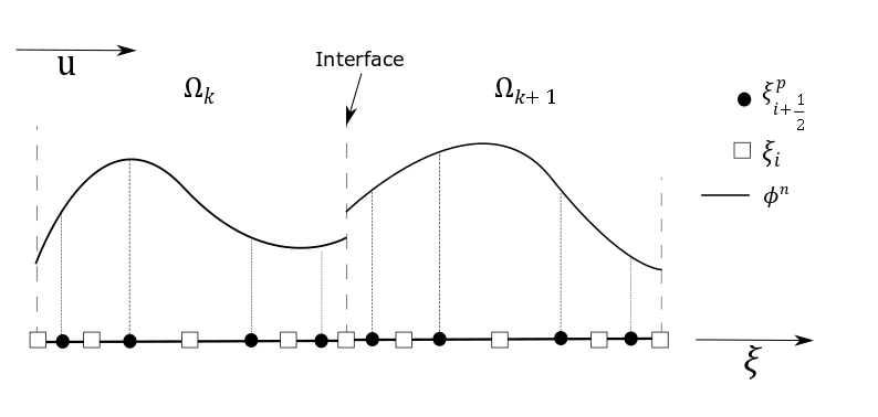
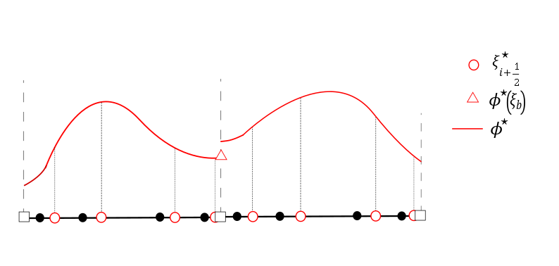
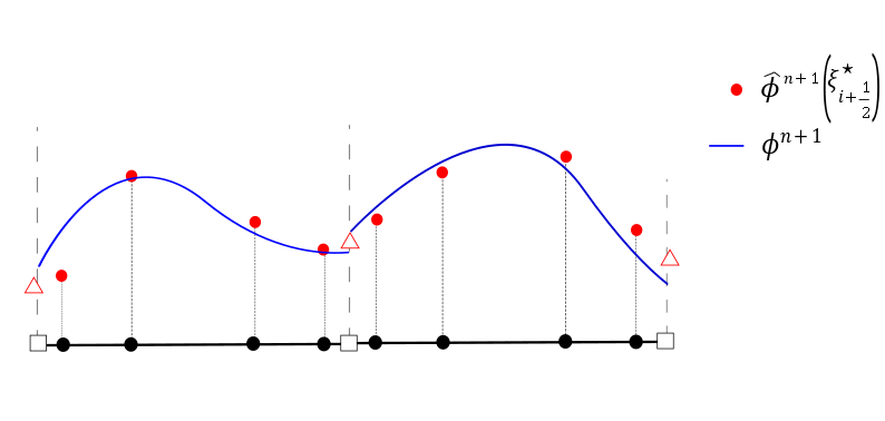
(a) Initialization at Gauss points (b) Particle advection (c) Remapping to Gauss points

Figure 1: Schematic of the DSEM SL method: (a) The tracer particles are initialized on each subdomain at the Chebyshev Gauss points, $\xi_{i+1/2}^{p}$; (b) the particles are traced forward in time to obtain the advected location, $\xi^{\star}_{i+1/2}$, the advected solution, $\phi^{\star}$, and the the interface solution, $\phi^{\star}(\xi_{b})$; (c) the solution is remapped to obtain the intermediate solution at original tracer locations, $\hat{\phi}^{n+1}(\xi_{i+1/2}^{p})$. Using a least squares fit with constraint for the boundary condition, and for mass and/or energy conservation, we obtain the solution $\phi^{n+1}$.

4.1 Solution initialization

To be consistent with an Eulerian solver, we initialize $N$ particles within a subdomain, $k$, at time $t^{n}$ at the Gauss quadrature collocation points in (9). The solution, $\phi^{n}$, is then approximated by a Lagrange interpolant as follows,

$$\phi^{n}(\xi)=\sum\limits_{i=0}^{N-1}{\phi}^{n}(\xi^{p}_{i+1/2})h_{i+1/2}(\xi),$$ (13)

where $h_{i+1/2}(\xi)$ are the Lagrange polynomials of degree $N-1$ defined on the Chebyshev Gauss points $\xi_{i+1/2}^{p}$ according to

$$h_{i+1/2}(\xi)=\prod_{\begin{subarray}{c}i=0\\ i\neq j\end{subarray}}^{N-1}\frac{\xi-\xi^{p}_{i+1/2}}{\xi^{p}_{j+1/2}-\xi^{p}_{i+1/2}},\qquad j=0,1,...,N-1.$$ (14)

The solution $\phi$ is initialized at $t^{0}$=0 as ${\phi}^{0}(\xi^{p}_{i+1/2})$.

4.2 Forward time integration

The particle variable, $\phi^{n}$, is advected in time along its characteristic path according to (6). We update each particle’s location, i.e.

$$\frac{d\xi^{p}_{i+1/2}}{dt}=u(\xi^{p}_{i+1/2})\qquad i=0,1,...,N-1,$$ (15)

with an explicit time integration, so

$$\xi^{\star}_{i+1/2}=\xi^{p}_{i+1/2}+\Delta tu(\xi^{p}_{i+1/2})\qquad i=0,1,...,N-1,$$ (16)

where $\xi^{\star}$ is the advected particle location at $t^{n+1}$. In this paper, we take $u(\xi_{i+1/2})$ prescribed, but in a general Eulerian-Lagrangian formulations it is a velocity interpolated from the Eulerian grid based solver. Because the particles are seeded at the Gauss quadrature points, the velocity at those location is conveniently and directly available (without interpolation) from the DSEM solver.

An explicit time integration is common for Eulerian-Lagrangian methods [15, 14, 13] In principle, any explicit integration scheme can be implemented for the DSEM solver and consistently for the semi-Lagrangian solver also. For simplicity of notation and for the sake of the concise presentation of the algorithm, we describe the semi-Lagrangian method using a first-order Euler scheme in (16). We have used several time integration schemes of higher order in the tests discussed in the sections below.

While there is no formal stability criterion for the temporal update of the linear characteristic equation, in order to prevent an advected particle from leaving a subdomain we restrict the time step nevertheless as follows

$$\Delta t\leq\frac{\Delta\xi_{\text{min}}}{|u|_{max}}.$$ (17)

Here, $\Delta\xi_{min}$ is the minimum grid spacing between two particles, i.e. Chebyshev quadrature points, at the edges of the subdomain and $|u|_{max}$ is the maximum advection speed. This time step limit is typically less restrictive than the explicit CFL time step for the Eulerian DSEM solver, because the latter time step is restricted by the same minimum grid spacing, $\xi_{min}$, but by the maximum of multiple characteristic velocities of the hyperbolic system. These velocities usually have a greater magnitude than $|u|_{max}$ and so the explicit time step for the semi-Lagrangian method is not-restrictive for a coupled EL formulation.

The benefit of preventing a particle from leaving the subdomain is two-fold. Firstly, information from the neighboring subdomains are not involved in the advection step and the remapping will require the solutions to be connected along the interface between subdomains only, i.e. the subdomains are non-overlapping. This yields a local method; again, consistent with DSEM. Secondly, with the advected particle locations within a subdomain deviating only marginally from the quadrature points, we find that the advected polynomial is not ill-posed.

The solution after advection is denoted by $\phi^{\star}(\xi)$ and is given as

$$\phi^{\star}(\xi)=\sum\limits_{i=0}^{N-1}{\phi^{\star}}(\xi^{\star}_{i+1/2})h^{\star}_{i+1/2}(\xi),$$ (18)

where $h^{\star}_{i+1/2}(\xi)$ are the Lagrange polynomials of degree $N-1$ defined on the advected points $\xi_{i+1/2}^{\star}$,

$$h^{\star}_{i}(\xi)=\prod_{\begin{subarray}{c}i=0\\ i\neq j\end{subarray}}^{N-1}\frac{\xi-\xi^{\star}_{i+1/2}}{\xi^{\star}_{j+1/2}-\xi^{\star}_{i+1/2}},\qquad j=0,1,...,N-1.$$ (19)

The advected polynomial’s nodal solution values, ${\phi^{\star}}(\xi_{i+1/2}^{\star})$ are obtained by integrating $\phi^{n}(\xi_{i+1/2}^{n})$ along the characteristic curve according to (7),

$${\phi^{\star}}(\xi^{\star}_{i+1/2})={\phi}^{n}(\xi^{p}_{i+1/2})+\Delta t\left(-{\phi}^{n}(\xi^{p}_{i+1/2})\left(\frac{\partial u}{\partial\xi}\right)^{n}_{i+1/2}\right).$$ (20)

Here, we take $\left(\frac{\partial u}{\partial\xi}\right)^{n}_{i+1/2}$ prescribed from a hypothetical Eulerian grid based solver.

4.3 Remapping

Finally, in a remapping stage the advected polynomial is projected back onto the Gauss-Chebyshev quadrature nodes through interpolation as follows,

$$\phi^{\star}(\xi^{p}_{i+1/2})=\sum\limits_{j=0}^{N-1}{\phi^{\star}}(\xi^{\star}_{j+1/2})h^{\star}_{j+1/2}(\xi^{p}_{i+1/2}),$$ (21)

providing an estimate for the solution at time step, $n+1$, as follows

$$\widehat{\phi}^{n+1}(\xi_{j+1/2}^{p})=\phi^{\star}(\xi^{p})\qquad j=0,1,...,N-1.$$ (22)

Here, we use the hat symbol to denote the intermediate solution at $t^{n+1}$. To account for connectivity between elements, boundary conditions and conservation of mass, we constrain this intermediate solution. We then use a least-squares projection to obtain a corrected solution at $t^{n+1}$.

Boundary conditions and interface constraints can be applied either using backtracking on the characteristic line or by interpolation. To find the interface value $\hat{\phi}^{n+1}(\xi_{b})$, we trace a characteristic passing through $\xi_{b}$ backward in time as is illustrated in Figure 2. We locate the origin of the characteristic using $\xi^{\star}=\xi_{b}-u\Delta t$. The solution is then interpolated at $\xi^{\star}_{b}$, using the known solution at the quadrature nodes at $t^{n}$, $\phi^{n}(\xi_{i+1/2})$. [4].

$$\hat{\phi}^{n+1}_{b} = \sum\limits_{j=0}^{N-1}{\phi}^{n}(\xi^{p}_{j})h_{j}(\xi_{b}-u\Delta t)\qquad u>0\qquad b=1,2.$$ (23)

where the subscript $b$=1,2 identifies an interface value or coordinate at the left or right end of the subdomain, respectively.

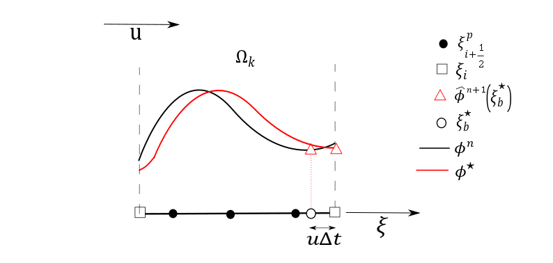
Figure 2: Schematic of backward tracing procedure to determine interface values of the solution: to determine the interface value $\hat{\phi}^{n+1}(\xi_{b})$, a characteristic is traced backward in time that passes through $\xi_{b}$.The origin of the characteristic is located using $\xi^{\star}=\xi_{b}-u\Delta t$. The solution is then interpolated at $\xi^{\star}_{b}$, using the known solution at the quadrature nodes at $t^{n}$, $\phi^{n}(\xi_{i+1/2})$ .

Alternatively, we can determine the boundary values using polynomial interpolation according to (18),

$$\hat{\phi}^{n+1}_{b}=\sum\limits_{j=0}^{N-1}{\phi^{\star}}(\xi^{\star}_{j+1/2})h^{\star}_{j+1/2}(\xi_{b})\qquad b=1,2$$ (24)

By upwinding, a unique interface value is determined from the interfaces values of two neighbouring subdomains

$$\hat{\phi}^{n+1}_{b\star}=f\left(\hat{\phi}^{n+1}_{b=1}\bigg{|}_{\Omega_{k}},\hat{\phi}^{n+1}_{b=2}\bigg{|}_{\Omega_{k-1}}\right)$$ (25)

Boundary conditions are implemented in the same way as interface condition by using a specified ghost solution at computational domains boundaries.

In the tests conducted below, we compare the backtracing and interpolation approaches and find that they produce similar results.

Mass and Energy Conservation

Local mass conservation

With the above remapping, mass is not exactly conserved. An additional constraint for local mass conservation can be imposed as follows. Using the equivalent Eulerian formulation in (4), an expression for the mass in a subdomain is given by

$$\frac{\partial}{\partial t}\int_{\Omega_{k}}\phi dx=-u\left.\phi\right|^{\xi_{b=2}}_{\xi_{b=1}}.$$ (26)

Here, $M$ is the mass, $M=\int_{\Omega_{k}}\phi dx$ and $\mathcal{F}_{x}$ is the mass flux, $\mathcal{F}_{x}=u\left.\phi\right|^{\xi_{b=2}}_{\xi_{b=1}}$. The integral is numerically evaluated using Gauss quadrature,

$$M^{n}=\sum\limits_{j=0}^{N-1}w_{j+1/2}{\phi}^{n}(\xi_{j+1/2})\qquad j=0,1,...,N-1,$$ (27)

where $w_{j+1/2}$ are the quadrature weights. We find the mass at $M^{n+1}$ through time integration,

$$M^{n+1}=M^{n}-\mathcal{F}_{m}^{n}\Delta t,$$ (28)

with the flux $\mathcal{F}_{m}^{n}=u\phi^{n}_{b=1}-u\phi^{n}_{b=2}$ The boundary values, $\phi^{n}_{b}$, at $t^{n}$ are determined with interpolation from the polynomial defined on the Gauss qaudrature nodes.

Local energy conservation

Just like mass, energy is not exactly conserved. An additional constraint for local energy conservation with a constant velocity advection can be formulated as follows,

$$\frac{\partial}{\partial t}E=-u\left.\phi^{2}\right|^{x_{\text{b=2}}}_{x_{\text{b=1}}},$$ (29)

where $E=\int_{\Omega_{k}}\phi^{2}dx$. The integral is evaluated using Gauss quadrature. Because the energy is non-linear (quadratic in $\phi$), we have to iterate to solve the constrained system that will be discussed below. For that purpose we introduce the $k$ counter as follows

$$E^{n}=\sum\limits_{j=0}^{N-1}w_{j+1/2}\widehat{\phi}^{(k-1)}(\xi_{j+1/2})\widehat{\phi}^{(k)}(\xi_{j+1/2})\qquad j=0,1,...,N-1,$$ (30)

The iteration is terminated when $|\widehat{\phi}^{(k-1)}-\widehat{\phi}^{(k)}|<10^{-8}$. For a first order time integration and a constant $u$, the energy at time $t^{n+1}$ is determined as,

$$E^{n+1}=E^{n}-\Delta t\mathcal{F}_{e}^{n},$$ (31)

where $\mathcal{F}_{e}^{n}=u\left.\left(\phi^{n}\right)^{2}\right|^{x_{\text{b=2}}}_{x_{\text{b=1}}}$.

Least-squares solution of the constrained system

To project the interpolated polynomial, $\hat{\phi^{n+1}}$, combined with the constraints onto the Gauss-Chebyshev quadrature using a least-squares method, an overdetermined system of equations has to be solved. The number of equations depends on the number of constraint equations included. For example, if the boundary constraint and the local mass and energy constraint equations are used, Equations (22), (24), (28) and (31) form a system of equations with $N$+4 equations and $N$ unknowns. We write the system of equations in matrix form as follows;

$$\begin{bmatrix}1&0&\dots&0\\ 0&1&\dots&0\\ \vdots\\ 0&0&\dots&1\\ h_{1/2}(\xi_{b=2})&h_{3/2}(\xi_{b=2})&\dots&h_{N-1/2}(\xi_{b=2})\\ h_{1/2}(\xi_{b=1})&h_{3/2}(\xi_{b=1})&\dots&h_{N-1/2}(\xi_{b=1})\\ w_{1/2}&w_{3/2}&\dots&w_{N-1/2}\\ A_{1/2}&A_{3/2}&\dots&A_{N-1/2}\end{bmatrix}\begin{bmatrix}{\phi}^{n+1}(\xi^{p}_{1/2})\\ {\phi}^{n+1}(\xi^{p}_{3/2})\\ \vdots\\ {\phi}^{n+1}(\xi^{p}_{N-1/2})\end{bmatrix}=\begin{bmatrix}\widehat{\phi}^{n+1}(\xi_{1/2}^{p})\\ \widehat{\phi}^{n+1}(\xi_{3/2}^{p})\\ \vdots\\ \widehat{\phi}^{n+1}(\xi_{N-1/2}^{p})\\ \widehat{\phi}^{n+1}_{b\star=1}\\ \widehat{\phi}^{n+1}_{b\star=2}\\ M^{n}+\Delta t\mathcal{F}_{m}^{n}\\ E^{n}+\Delta t\mathcal{F}_{e}^{n}\\ \end{bmatrix}$$ (32)

Here, we use the notation $A_{i+1/2}=w_{i+1/2}\phi^{k-1}(\xi^{p}_{i+1/2})$ to prevent clutter in (32). If the energy constraint is enforced, then an iterative solution to the system is necessary and the superscript on the $\hat{\phi}$ should be $k$ rather than $n+1$. The counter $k$ is the iteration number. If the energy constraint is not enforced, then the last row disappears and the system can be solved directly. A Least squares fit is used to solve the over determined system to obtain ${\phi}^{n+1}(\xi_{j}^{p})$.

Two dimensional scheme

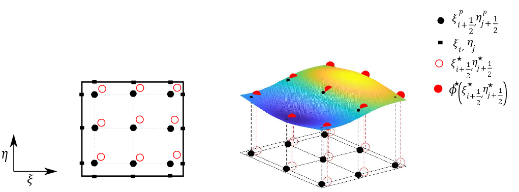
Figure 3: Schematic of the DSEM SL method in two dimensions. The solution,$\phi^{n}$ is initialized on the Gauss nodes, $\xi^{p}_{i+1/2},\eta^{p}_{j+1/2}$. A 2D interpolant constructed at the Gauss nodes to obtain the intermediate solution using the advected solution, $\phi^{\star}$ on the advected positions, $\xi^{\star}_{i+1/2},\eta^{\star}_{j+1/2}$.

Similar to the one dimensional scheme, in two dimensions the particles are initialized at the Gauss quadrature points, but along tensorial grid lines (Fig. 3),

$$\phi^{n}(\xi,\eta)=\sum\limits_{i=0}^{N-1}\sum\limits_{j=0}^{N-1}{\phi}^{n}(\xi^{p}_{i+1/2},\eta^{p}_{j+1/2})H_{i+1/2,j+1/2}(\xi,\eta),$$ (33)

where $H_{i+1/2j+1/2}(\xi,\eta)=h_{i+1/2}(\xi)h_{j+1/2}(\eta)$ and $h_{i+1/2}(\xi)$ and $h_{j+1/2}(\eta)$ are the Lagrange polynomials of degree $N-1$ along the $\xi$ and $\eta$ directions respectively. Forward time integration of the particles is performed in $x$- and $y$- directions using the velocities $u(\xi^{p}_{i+1/2},\eta^{p}_{j+1/2})$ and $v(\xi^{p}_{i+1/2},\eta^{p}_{j+1/2})$, respectively, as prescribed or interpolated from an Eulerian formulation. The advected particle positions and solutions so obtained are denoted as $\xi^{\star}_{i+1/2},\eta^{\star}_{j+1/2}$ and $\phi^{\star}(\xi^{\star}_{i+1/2},\eta^{\star}_{j+1/2})$, respectively.

Up to this point, the algorithm is exactly like the one-dimensional algorithm but along tensorial grid lines. The interpolation in two dimensions is more intricate as compared to the one dimensional algorithm. Instead of using an interpolant based on advected nodal values, a two-dimensional interpolant defined at the tensor grid of Gauss quadrature points is used to determine the intermediate solution, $\widehat{\phi}^{n+1}$.

$$\phi^{\star}(\xi^{\star}_{i+1/2},\eta^{\star}_{j+1/2})=\sum\limits_{l=0}^{N-1}\sum\limits_{m=0}^{N-1}\widehat{\phi}^{n+1}(\xi^{p}_{l+1/2},\eta^{p}_{m+1/2})H_{l+1/2,m+1/2}(\xi_{i+1/2}^{\star},\eta_{j+1/2}^{\star}),$$ (34)

$$\qquad i,j=0,1,...,N-1.$$

The interpolation then comes down to determining $\widehat{\phi}^{n+1}$ by inverting the matrix defined by $H_{l+1/2,m+1/2}(\xi^{\star}_{i+1/2},\eta^{\star}_{j+1/2})$ at every time step,
$\left[\begin{array}[]{llcl}H_{1/2,1/2}(\xi_{1/2}^{\star},\eta_{1/2}^{\star})&H_{1/2,3/2}(\xi_{1/2}^{\star},\eta_{1/2}^{\star})&\dots&H_{N+1/2,N+1/2}(\xi_{1/2}^{\star},\eta_{1/2}^{\star})\\ H_{1/2,1/2}(\xi_{1/2}^{\star},\eta_{3/2}^{\star})&H_{1/2,3/2}(\xi_{1/2}^{\star},\eta_{3/2}^{\star})&\dots&H_{N+1/2,N+1/2}(\xi_{1/2}^{\star},\eta_{3/2}^{\star})\\ \vdots\\ H_{1/2,1/2}(\xi_{N+1/2}^{\star},\eta_{N+1/2}^{\star})&H_{1/2,3/2}(\xi_{N+1/2}^{\star},\eta_{N+1/2}^{\star})&\dots&H_{N+1/2,N+1/2}(\xi_{N+1/2}^{\star},\eta_{N+1/2}^{\star})\end{array}\right]$

For the matrix to not be ill-posed the particles should not cross each other or stray to far from the quadrature points, on which we know that the interpolant is well-defined. To keep the particles close to the quadrature points, we restrict the time step as follows,

$$\Delta t\leq\text{min}\left[\frac{\Delta\xi_{\text{min}}}{|u|_{max}},\frac{\Delta\eta_{\text{min}}}{|v|_{max}}\right].$$ (35)

With this restriction particles cannot leave the subdomain. In the interior of the subdomain the spacing between the quadrature nodes is quite a bit larger and the particles remain relatively close to the quadrature nodes. Here, $\Delta\xi_{min}$ and $\Delta\eta_{min}$ are the minimum grid spacing between two particles and $|u|_{max}$ and $|v|_{max}$ are the maximum advection speed along $\xi$ and $\eta$ directions, respectively. Like for the one-dimensional scheme, this time step limit is typically less restrictive than the explicit CFL time step for the Eulerian DSEM solver. Once the intermediate solution $\hat{\phi}^{n+1}$ is obtained, we use 1D Lagrange polynomials to interpolate at the interface and boundary points.

$$\hat{\phi}^{n+1}_{j}|_{b}=\sum\limits_{i=0}^{N-1}{\hat{\phi}^{n+1}}(\xi_{i+1/2},\eta_{j+1/2})h_{i+1/2}(\xi_{b})\qquad j=0,1,..N-1$$ (36)

$$\qquad b=1,2$$

$$\hat{\phi}^{n+1}_{i}|_{b}=\sum\limits_{j=0}^{N-1}{\hat{\phi}^{n+1}}(\xi_{i+1/2},\eta_{j+1/2})h_{j+1/2}(\eta_{b})\qquad i=0,1,..N-1$$ (37)

$$\qquad b=3,4$$

where $b=1,2$ are the interface and boundary points along $\xi$ direction and $b=3,4$ are the interface and boundary points along $\eta$ direction. The final step is to use a least squares remapping.

5 Numerical tests

We test the semi-Lagrangian scheme for combinations of accuracy of the time integrator and mass and/or energy constraints as listed in Table 1. We consider a one-dimensional constant velocity advection, a non-constant velocity advection and a two-dimensional constant velocity advection case. The tests and their results are discussed in the sections below.

Case	Time integration order	Mass constraint	Energy constraint
Basecase1	First	-	-
MF1	First	Included	-
MEF1	First	Included	Included
Basecase2	Second	-	-
MF2	Second	Included	-
MEF2	Second	Included	Included
MF3	Third	Included	-

Table 1: Definition of acronyms used to describe combinations of accuracy of the time integration and types of constraints.

In each of the tests, we inspect the behavior of local errors and global (error) norms. We consider the $L_{2}$ error norm which is calculated by summing up local $L_{2}$ error norms in each subdomain, $k$, as,

$$\|e\|_{L^{2}}=\sum\limits_{k=1}^{K}\sqrt{\int_{\Omega_{k}}(\phi-\phi_{\text{exact}})^{2}d\xi}.$$ (38)

The conservation properties of the method are inspected with the following global mass and energy norms,

$$\|M\|=\sum\limits_{k=1}^{K}\frac{\int_{\Omega_{k}}\phi d\xi}{\int_{\Omega_{k}}\phi_{\text{exact}}d\xi},$$ (39)

and

$$\|E\|=\sum\limits_{k=1}^{K}\frac{\int_{\Omega_{k}}\phi^{2}d\xi}{\int_{\Omega_{k}}\phi^{2}_{\text{exact}}d\xi}.$$ (40)

respectively. For the test cases in which the analytic global mass is zero, we adjust the definition of the global mass norm as follows $\|M_{r}\|=\sum\limits_{k=1}^{K}\int_{\Omega_{k}}\phi d\xi$ to avoid division by zero.

We expect that the accuracy of the scheme depends on the interpolation and time integration accuracy and the impact of the constraints through the least squares fitting. We will discuss error and stability behavior by means of the test below.

5.1 One dimensional constant velocity

As a first test, we consider a linearly advected sine wave according to (6) and (7) with $u$=1 in a domain $x$=$[0,1]$. The initial condition is $\phi(x,0)$ =$\sin(2\pi x)$. Periodic boundary conditions are specified so that the sine wave propagates through the domain. Simulations are run until $T=$10, at which time error norms are determined and compared for several variations of the numerical scheme according to Table 1. Tests are conducted for polynomial orders of $P$=4,5,6, and 7 with different number of elements, $H$=4,5,6, and 7.

Because the advection velocity is constant, the time integration of the particle’s location is exact, independent of the accuracy of the time integration. The accuracy of the Basecases (Table 1) which only use the boundary constraint in the least squares fit step of the algorithm do not depend on the time integrator. So, the time evolution of the global norms for the Basecases as shown in Figure 4b, c and d for a case with $H$=4 and $P$=6, do not depend on the accuracy of the time integrator. We hence also observe that the results at $T$=10 of Basecase1 and Basecase2 in Figure 4a overlap each other.

The temporal update of mass and energy in (28) and (31) used as constraints in (32) do depend on the accuracy of the time integrator. The first order schemes, which can be expected to introduce a time integration error on the order of the explicit stable time step, which is $\Delta t={O}(10^{-3})$ for this case, yield a global $L^{2}$ error at $T$=10 of $\mathcal{O}(10^{-1})$ for both mass and energy constraint cases (Fig. 4b) . While the mass norms are constant (Fig. 4c), the energy norms (Fig. 4 d) are not conserved and, in fact, increase over time. This is further confirmed by the increased amplitude of the sine wave in the solution at $T$=10 in Figure 4a. Clearly, the local time error accumulates in time and the first order temporal update of the constraint in combination with the least squares fit is leading to a significant increased error as compared to the Basecases.Using the second order time integration, improves the $L^{2}$ error for the MF2 cases, i.e. the mass flux constraint. Moreover, for this case the global energy conservation is accurate.

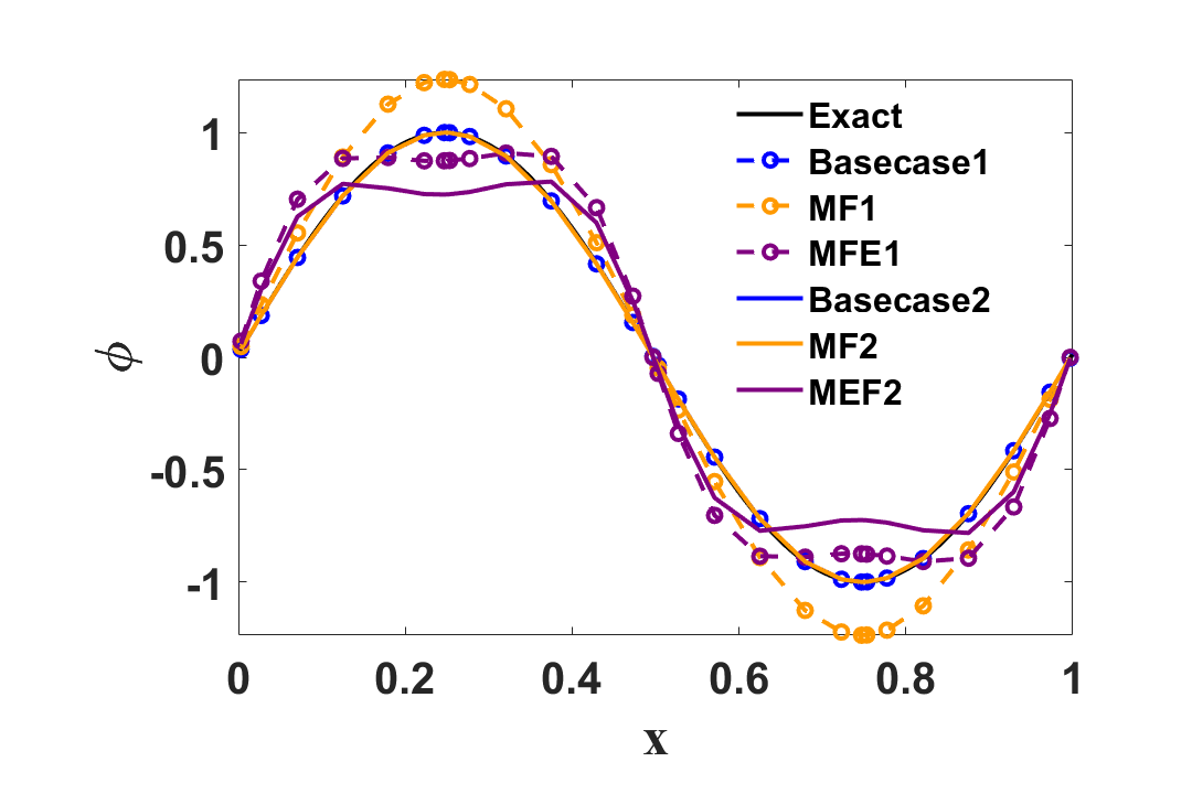
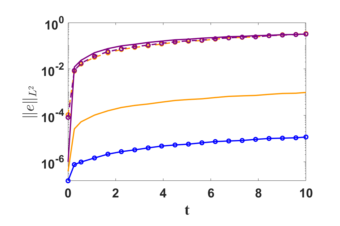
        (a)         (b)

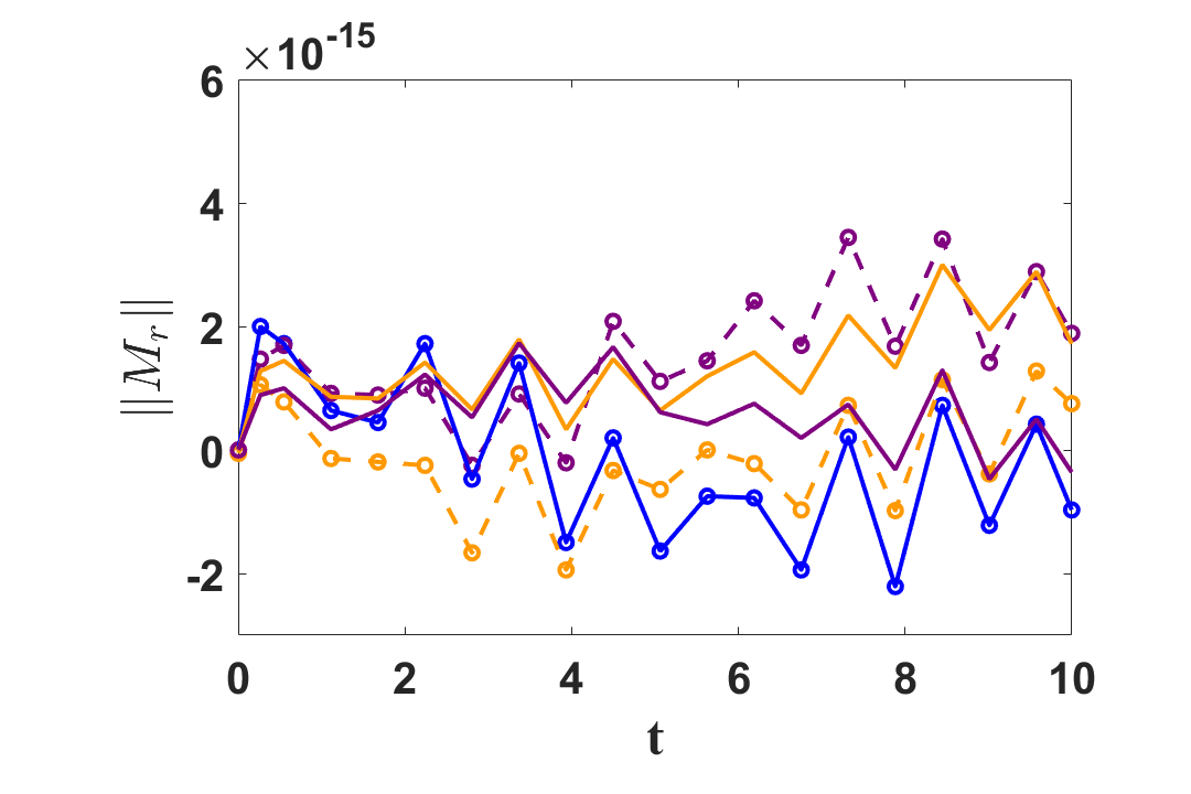
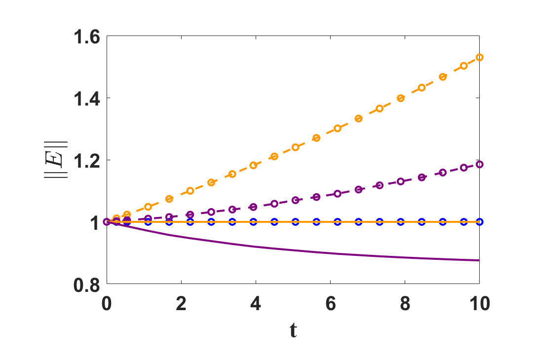
        (c)         (d)

Figure 4: Results for a linearly advected sine wave with DSEM-SL using $H$=4 subdomains and an approximation order of $P$=6; (a) the solution, $\phi$, versus $x$ at $T$=10. The $L^{2}$ error norm, $\|e\|_{L^{2}}$, the mass norm, $\|M\|$, and the energy norm, $\|E\|$ are plotted versus time, $t$, in subfigures (b), (c) and (d), respectively.

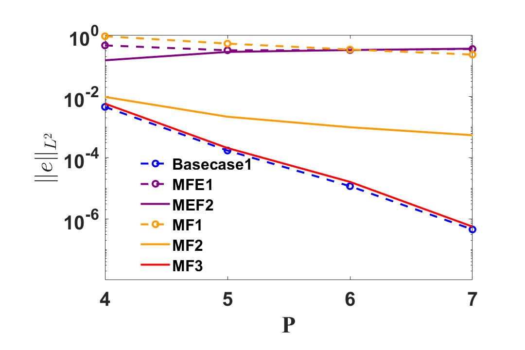
Figure 5: $P$-convergence of the schemes in Table 1 for a constant velocity linearly advected sine wave using $H$=4 subdomains at $T$=10 using the explicit stable time step.

Enforcing the additional constraint on the local energy (MEF2) produces spurious modes in the solution as observed in cases MEF1 and MEF2 shown in Figure 4a. It would appear that the extra energy constraint leads to the least-squares system being overconstrained, in turn, leading to instability. This is underscored by the non-conservation of the global energy for the MEF cases.

The $\|e\|_{L^{2}}$ plotted versus $P$ for $T$=10 in Figure 5 shows that the Base cases are exponentially convergent. While the mass and energy is not formally conserved for those cases, the high order convergence and accuracy translates to an accurate, spectral approximation of the mass and energy. The first-order MF1 case does not show $P$-convergence in Figure 5 because the overall error is bound by the accuracy of the time integrator. The second-order MF2, which is more accurate in time, does show an error improvement with $P$ that is algebraic. This is consistent with the algebraic convergence of the time integration and the stable time step reduction that is inherent to an increase of $P$. With a further increase of the time accuracy to third-order, the MF3 case matches the result of the Basecase, which is bound by the accuracy of the polynomial interpolation. Table, 2 shows that the Basecase methods exhibit formal $H$-convergence. The order of convergence is a little lower than $P$ which is the expected convergence rate. The MF1 and MF2 cases converge according to the order of time integration.

		$P$=4
		$\|e\|_{L^{2}}$	Slope
Basecase	$H$=5	$2.067\times 10^{-3}$	3.47
	$H$=6	$1.07\times 10^{-3}$	3.60
	$H$=7	$5.98\times 10^{-4}$	3.78
MF1	$H$=5	$8.02\times 10^{-1}$	0.57
	$H$=6	$7.38\times 10^{-1}$	0.45
	$H$=7	$6.65\times 10^{-1}$	0.67
MF2	$H$=5	$5.53\times 10^{-3}$	2.41
	$H$=6	$3.69\times 10^{-3}$	2.22
	$H$=7	$2.737\times 10^{-3}$	1.93
MF3	$H$=5	$2.64\times 10^{-3}$	3.47
	$H$=6	$1.39\times 10^{-3}$	3.52
	$H$=7	$7.92\times 10^{-4}$	3.65

Table 2: $H$ convergence of the $L^{2}$ error norm, $\|e\|_{L^{2}}$, for $P$=4 at $T$=10.

In Figure 6 we compare solutions obtained with two approaches to determine the interface solution that include the backtracking approach and the interpolation approach. These interface values are applied as the boundary constraint in the least squares fit. The $L^{2}$ error with $H$=4 with $P$=4,5,6, and7 shows that both methods show no distinguishable result. We find that the interpolation error is typically small and that it matches the solution from backtracking. The interpolation approach is easier to implement and we therefore prefer it.

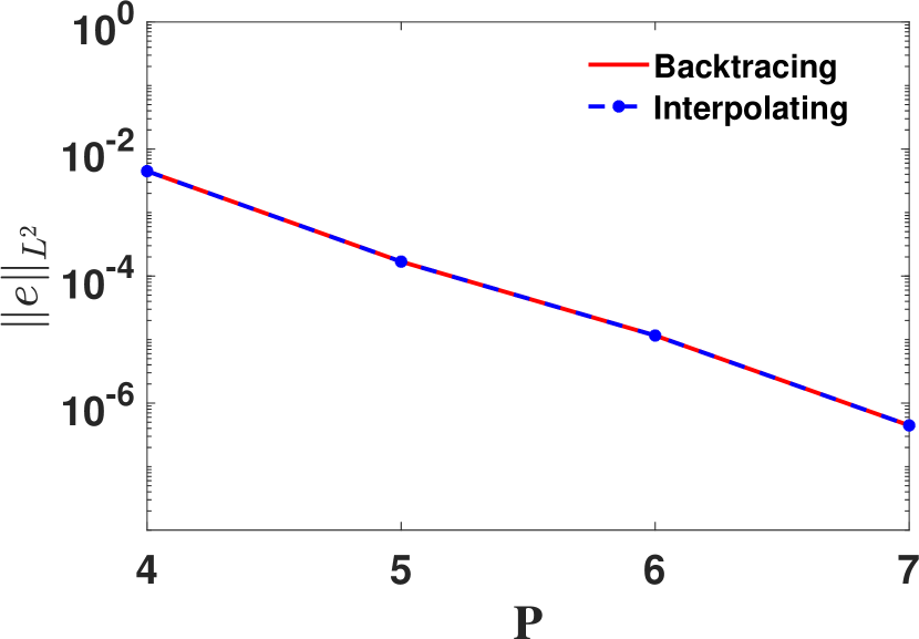
Figure 6: Simulation of constant velocity advection using DSEM-SL method using the explicit stable time step. Plot comparing the backtracking and interpolation boundary constraints when $H=4$ and $t=10$.

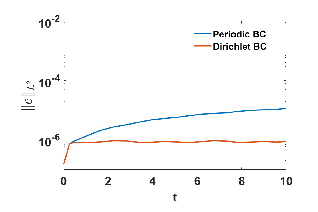
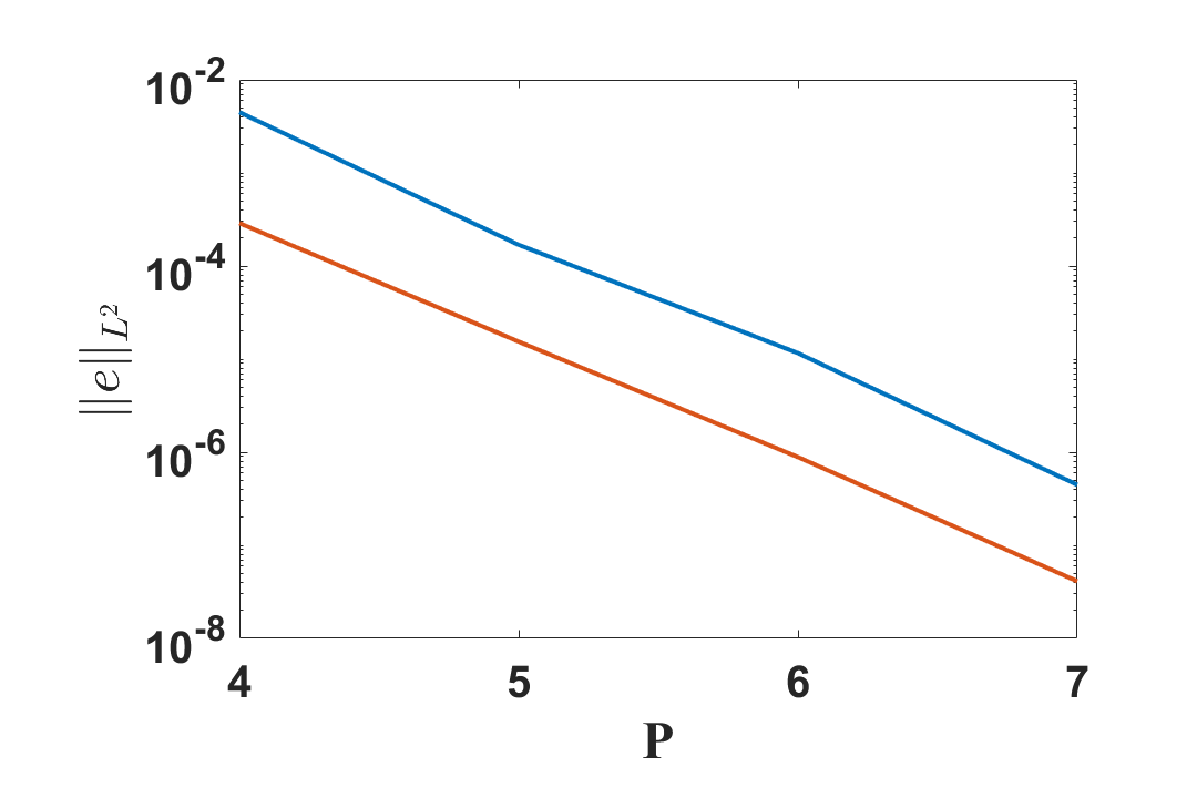
        (a)         (b)

Figure 7: Comparing Dirichlet and periodic boundary conditions using the Basecase for a constant velocity linearly advected sine wave. (a) shows the time evolution of the $\|e\|_{L^{2}}$ error using $P$=6 and $H$=4. (b) compares the $P$-comnvergence at $T$=10d.

As a last verification of the algorithm for the constant velocity case, we compare results obtained with a Dirichlet boundary condition those obtained with a periodic boundary condition that we have used thus far. Figure  7, shows that the Dirichlet boundary condition is slightly more accurate than the periodic boundary condition for the Basecase. This can be expected because the Dirichlet boundary condition is exact at the inflow, and from there errors accumulate/increase in space, whereas the periodic conditions do not have this exact reference and hence the errors are homogeneous in space.

5.2 One dimensional non-constant velocity

To study the effect of a non-constant advection velocity, we consider a problem that is commonly considered for semi-Lagrangian methods [24] and that solves the following conservation equation in Eulerian form

$$\frac{\partial\phi}{\partial t}+\frac{\partial(-\sin(x)\phi)}{\partial x}=0$$ (41)

on the domain $x\in[0,2\pi]$. The initial condition is

$$\phi(x,0)={{\sin\left(2\tan^{-1}\left[\exp(-1)\tan({x\over 2})\right]\right)}\over{\sin(x)}}.$$ (42)

Periodic boundary conditions are used. The problem has an analytical solution which is described by a symmetric distribution function which dampens into a constant valued solution over time.

We can rewrite (41) in non-conservation form as

$$\frac{\partial\phi}{\partial t}-\sin(x)\frac{\partial\phi}{\partial x}=\cos(x)\phi.$$ (43)

The equivalent Lagrangian form that we use as the governing equation for solution with the DSEM-SL method (following (6) and (7)), is

$$\frac{d\mathbf{x^{p}}(t)}{dt} = -\sin(x)$$

$$\frac{D\phi}{Dt} = -\cos(x)\phi$$ (44)

Hence, the advection velocity, $u$=$\sin(x)$, is non-constant. We note that the right-hand side of the $\phi$ equation is non-zero and will require a temporal update according to (20). For the constant velocity case discussed in the previous this section right hand side was zero, and the $\phi$ solution for that case is simply constant along its characteristic path.

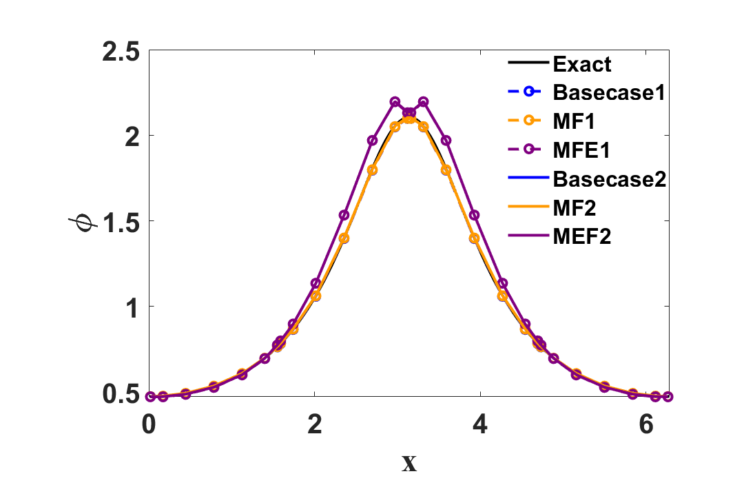
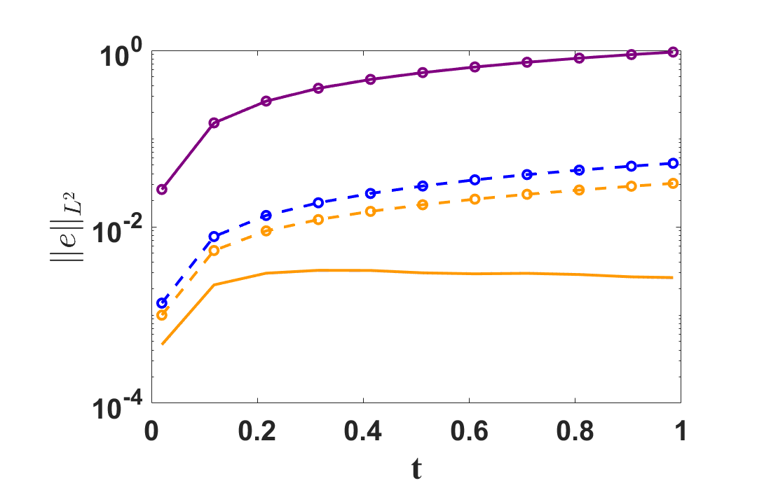
        (a)         (b)

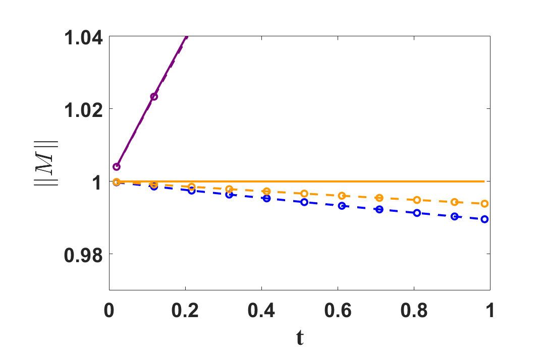
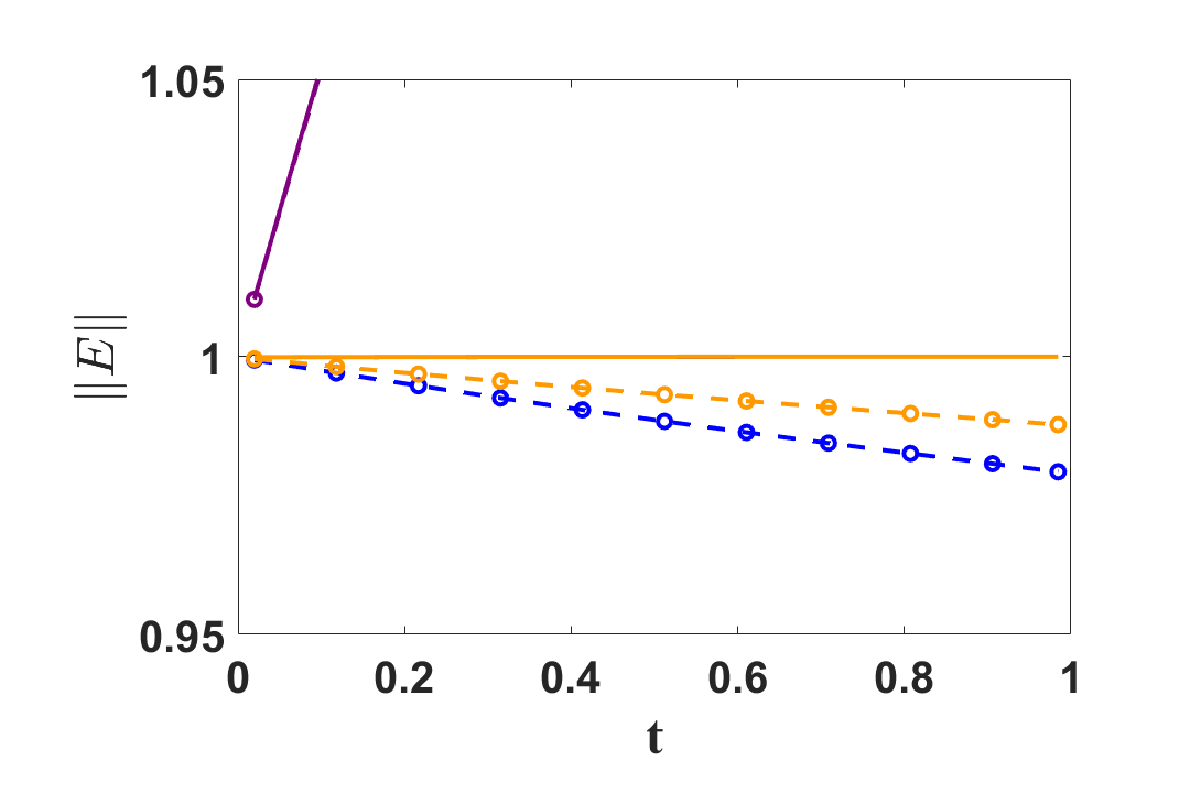
        (c)         (d)

Figure 8: Results for a non-constant velocity advection with DSEM-SL using $H$=4 subdomains and an approximation order of $P$=6; (a) the solution, $\phi$, versus $x$ at $T$=1. The $L^{2}$ error norm, $\|e\|_{L^{2}}$, the mass norm, $\|M\|$, and the energy norm, $\|E\|$ are plotted versus time, $t$, in subfigures (b), (c) and (d), respectively.

Figure 8 shows the results for a case with four subdomains and $P$=6. The explicit time step is $\Delta t$ is $1.97\times 10^{-2}$. As opposed to the constant velocity case in the previous section, the $\phi$ solutions of Basecase with non-constant velocity are dependent on the time integrator because of the non-zero right hand side in the $\phi$ equation in (5.2). The Basecase1 with a first order time integration has an $L^{2}$ error on the order of the time step of $\mathcal{O}(10^{-2})$ and is clearly bounded by the time integration error. The second order Basecase2 improves the accuracy to $\mathcal{O}(10^{-3})$ consistent with the increased time accuracy order. Because of the reduced accuracy for the first-order Basecase1, the global mass norm reduces by $2\%$ over the considered time interval of $T$=1 (See also Table 3). The second order Basecase2 conserves mass up to four decimals over $T$=1.

Case	$\|M\|$-1	$\|E\|$	$\|e\|_{L^{2}}$
Basecase1	-0.0104	0.9793	$5.25\times 10^{-2}$
MF1	-0.0061	0.9878	$3.11\times 10^{-2}$
MEF1	0.1334	1.3148	$9.57\times 10^{-1}$
Basecase2	0.0000	1.0000	$2.65\times 10^{-3}$
MF2	0.0000	1.0000	$2.65\times 10^{-3}$
MEF2	0.1367	1.3217	$9.56\times 10^{-1}$
MF3	0.0000	1.0000	$2.63\times 10^{-3}$

Table 3: Comparison of global for the non-constant advection velocity case at $T$=1 with $H$=4 and $P$=6.

The addition of a local mass constraint to the first order scheme, MF1 improves the global mass and energy conservation properties of the Basecase11 by $1\%$. The second order MF2 which includes the local mass constraint matches the solution of Basecase2. This is because the second order schemes reduce the time integration error to be on the order of $\mathcal{O}(10^{-4})$ and because the error is dominated by the interpolation error.

The addition of local energy constraints produces spurious modes which are observed in Figure 8a. This is similar to the constant advection velocity case. The overconstrained system is unstable as confirmed by the increase in relative global energy norm.

Figure 9a, which plots the approximation order $P$ against the $L^{2}$ error norm shows mostly algebraic convergence for the first order Basecase1 and MF1 methods. The second order methods Basecase2 and MF2 show spectral convergence in $P$ until $P$=10, when the time integration error bounds the error. The third-order, MF3 converges exponentially till $P$=12.

To understand the effect of time step, we consider a smaller time step $\Delta t$ = $10^{-4}$. Figure 9b shows that this indeed improves the convergence of the first order methods, and spectral convergence can be observed for this case up to $P$=8 where the error is of the order of $\mathcal{O}(10^{-4})$. Beyond $P$=8, the first order schemes are again bounded by the time integration error while the second and third order schemes continue to show spectral convergence.

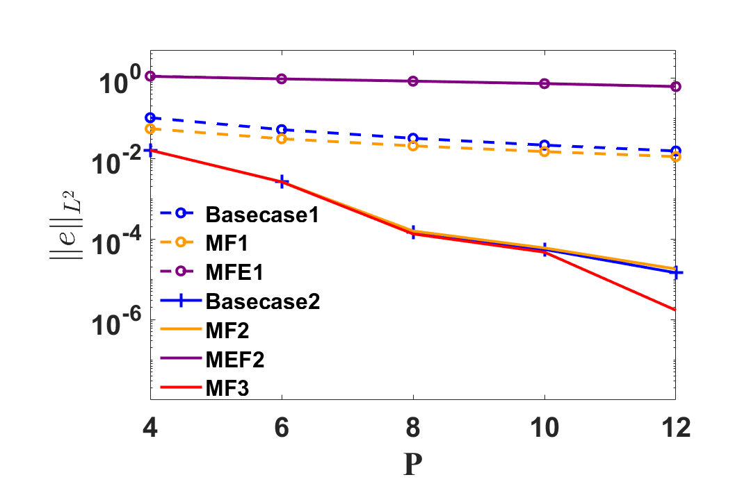
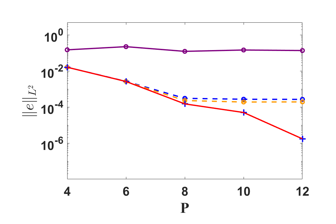
        (a)         (b)

Figure 9: $P$-convergence of the schemes in Table 1 for a non-constant velocity advection case using $H$=4 subdomains at $T$=1. for the explicit stable time step $\Delta t$ (a) and for a fixed time step $\Delta t$=$10^{-4}$(b)

5.3 Two dimensional constant velocity

To test the algorithm in two dimensions, we consider the two-dimensional constant velocity, linear advection equation in Lagrangian form

$${dx\over dt} = a$$

$${dy\over dt} = b$$

$${d\phi\over dt} = 0$$ (45)

We solve this equation on the domain $x$=[0,1],$y$=[0,1] with $a$=2, and $b$=1. An initial condition is set as $\phi(x,y,0)=\sin(2\pi x)\sin(2\pi y)$. Periodic boundary conditions are applied in both $x$- and $y$-directions. The simulation is carried out until time $T=1$.

Basecase1, Basecase2, MF1 and MF2 as listed in Table 1 are simulated for a number of subdomains in $x$- and $y$-directions of $H_{x}$=$H_{y}$=4,5,6, and 7 and approximation orders of $P$=4,5,6, and 7.

The time evolution of the conservative properties is shown in Figure 10. Since the velocity is constant, the time integration is exact in Basecase and Basecase2 and their solutions overlap each other, like for the one-dimensional case.

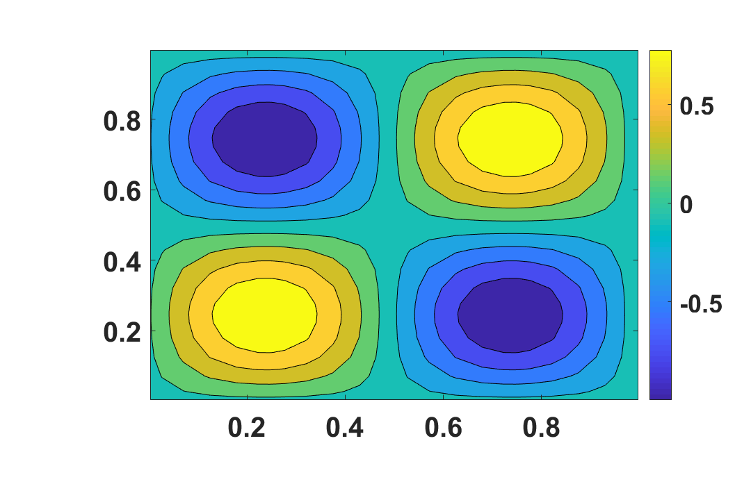
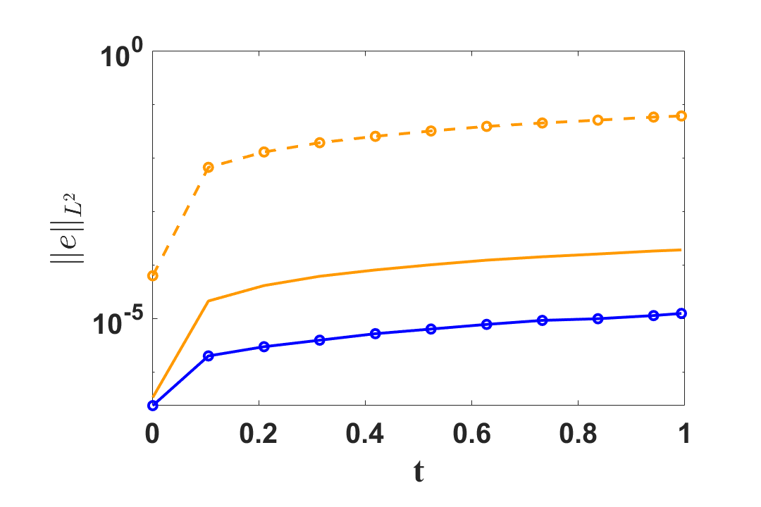
        (a)         (b)

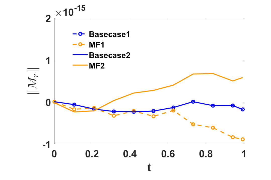
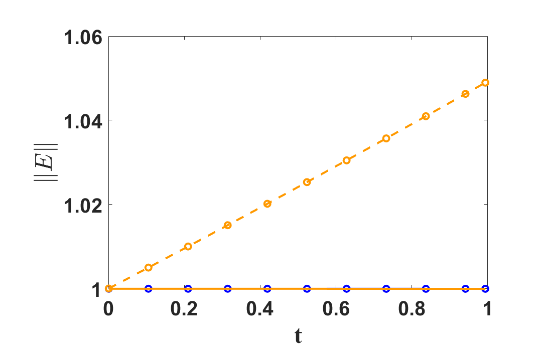
        (c)         (d)

Figure 10: Results for a two-dimensional constant velocity advection with DSEM-SL using $H$=4 subdomains in $x$- and $y$-direction and an approximation order of $P$=6 per subdomain; (a) the solution, $\phi$, versus $x$ at $T$=1. The $L^{2}$ error norm, $\|e\|_{L^{2}}$, the mass norm, $\|M\|$, and the energy norm, $\|E\|$ are plotted versus time, $t$, in subfigures (b), (c) and (d), respectively

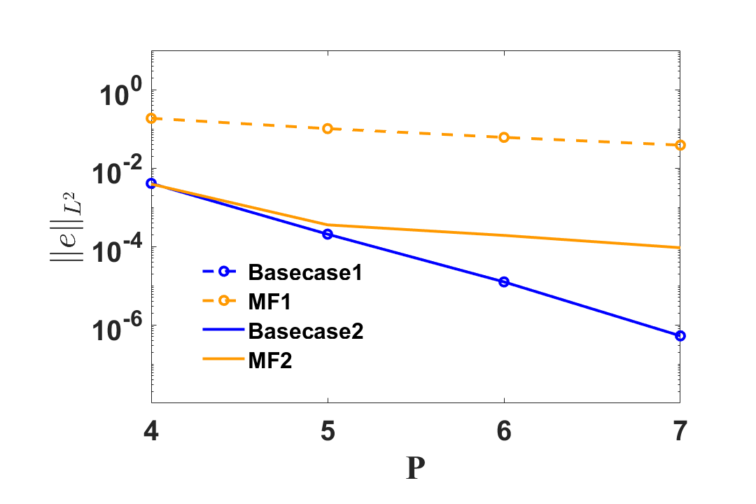
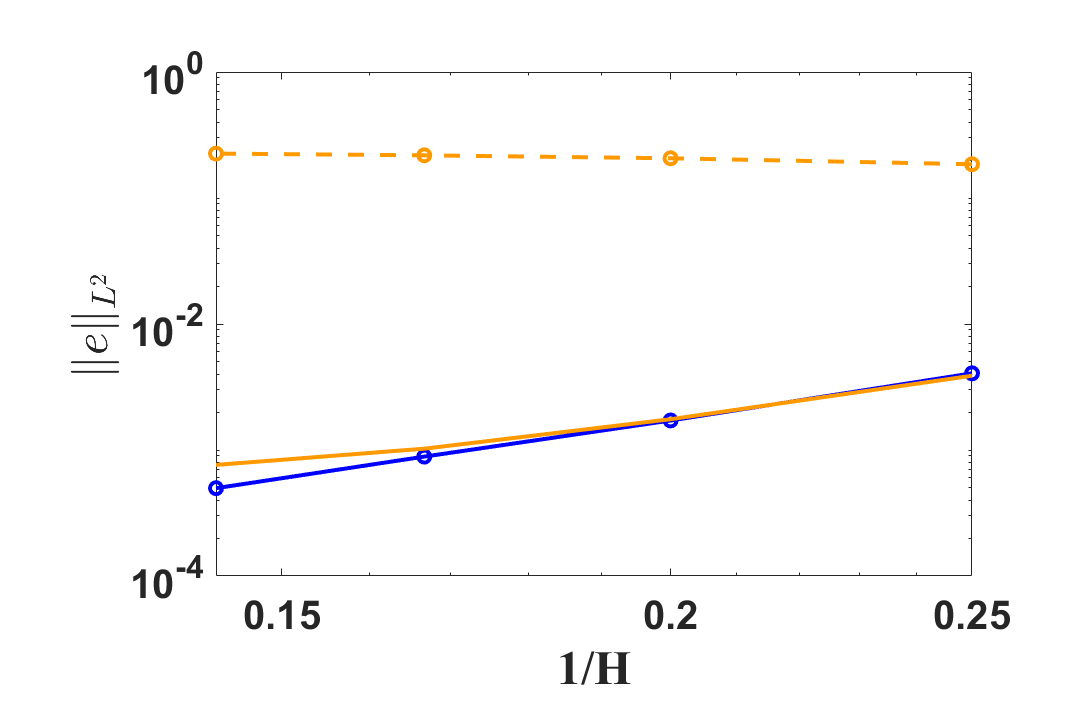
        (a)         (b)

Figure 11: $P$ convergence of the constant velocity 2D simulation using $H_{x}$=4, $H_{y}$=4 at $t$=1.

Addition of the local mass constraints with a first order time integration MF1, which introduces an error of order $\mathcal{O}(10^{-3})$ to the system of equations (32) leads to a global $L^{2}$ error of $\|e\|=\mathcal{O}(10^{-1})$. The MF1 scheme is non-conservative and gains $5\%$ energy over the time interval considered.

The second order method MF2, with a time integration error on the order of $\mathcal{O}(10^{-6})$, is more accurate with the $L^{2}$ error on the order of $\|e\|=\mathcal{O}(10^{-4})$.

Figure 11 shows that the $P$ and $H$ convergence of the cases at $T$=1 are similar to the 1D results. Basecase1 and Basecase2 show spectral $P$-convergence as well as algebraic $H$ convergence.

6 Conclusions

A high-order, explicit semi-Lagrangian method is developed to solve the Lagrangian transport equations in Eulerian-Lagrangian formulations. The semi-Lagrangian method is consistent with an explicit Eulerian solver discretized with an explicit discontinuous spectral element method (DSEM).

By seeding tracer particles at the Gauss quadrature nodes, the Lagrangian solution is directly available at quadrature nodes of the Eulerian solver and vice-versa. This is exchange of information is commonly performed using computationally intensive and complicated interpolation methods in Eulerian-Lagrangian formulations.

Consistent with DSEM, the semi-Lagrangian method is explicit. By choosing the explicit time step appropriately, particles are prevented from leaving the element. This ensures a local and parallel method, which is natural for DSEM.

Following the explicit trace, the solution is remapped to the original quadrature points using a least squares fit. This causes the method to loose formal conservation.

Mass and kinetic energy constraints were tested to correct for this conservation loss. The addition of a mass constraint does not improve mass conservation for cases with a constant advection velocity. For a non-constant advection velocity case, however, the mass constraints can improve conservation. In general, an increase of the time integration accuracy improves conservation and accuracy.

A kinetic energy constrains leads to an overconstraining of the system. The solution shows spurious oscillations and is unstable.

We are extending the current algorithm to solve stochastic differential equations in Eulerian-Lagrangian formulations and plan to report on this in the near future.

References

- [1] C. Birdsall and A. Langdon, Plasma physics via computer simulation, The Adam Hilger series on plasma physics, McGraw-Hill, 1985.
- [2] P. A. Bosler, J. Kent, R. Krasny, and C. Jablonowski, A Lagrangian particle method with remeshing for tracer transport on the sphere, Journal of Computational Physics, 340 (2017), pp. 639 – 654.
- [3] A. J. Chorin, Numerical study of slightly viscous flow, Journal of Fluid Mechanics, 57 (1973), p. 785–796.
- [4] N. Crouseilles, T. Respaud, and E. Sonnendrücker, A forward semi-Lagrangian method for the numerical solution of the Vlasov equation, Computer Physics Communications, 180 (2009), pp. 1730 – 1745.
- [5] C. Crowe, J. Schwarzkopf, M. Sommerfeld, and Y. Tsuji, Multiphase Flows with Droplets and Particles, Boca Raton: CRC Press, 2012.
- [6] J. K. Dukowicz and J. W. Kodis, Accurate conservative remapping (rezoning) for arbitary Lagrangian-Eulerian computations, SIAM Journal on Scientific and Statistical Computing, 8 (1987).
- [7] P. Frolkovič, Flux-based methods of characteristics for coupled transport equations in porous media, Computing and Visualization in Science, 6 (2004), pp. 173–184.
- [8] F. X. Giraldo, The Lagrange–Galerkin spectral element method on unstructured quadrilateral grids, Journal of Computational Physics, 147 (1998), pp. 114–146.
- [9] F. X. Giraldo, J. B. Perot, and P. F. Fischer, A spectral element semi-Lagrangian (SESL) method for the spherical shallow water equations, Journal of Computational Physics, 190 (2003), pp. 623–650.
- [10] W. Guo, R. D. Nair, and J.-M. Qui, A conservative semi-Lagrangian discontinuous Galerkin scheme on the cubed sphere, Monthly Weather Review, 142 (2014).
- [11] Gustaaf. B. Jacobs and David. A. Kopriva and Farzad Mashayek, Towards efficient tracking of inertial particles with high-order multidomain methods, Journal of Computational and Applied Mathematics, 206 (2007), pp. 392–408.
- [12] J. Hesthaven and T. Warburton, Nodal discontinuous Galerkin methods: algorithms, analysis, and applications, Springer-Verlag, Berlin, 2008.
- [13] G. Jacobs and W. Don, A high-order WENO-Z finite difference based Particle-Source-in-Cell method for computation of particle-laden flows with shocks, Journal of Computational Physics., 228 (2009).
- [14] G. Jacobs and J. Hesthaven, Implicit-explicit time integration of a high-order particle-in-cell method with hyperbolic divergence cleaning, Computer Physics Communications, 80 (2009).
- [15] G. B. Jacobs and J. S. Hesthaven, High-order nodal discontinuous Galerkin particle-in-cell method on unstructured grids, Journal of Computational Physics, 214 (2006), pp. 96–121.
- [16] G. B. Jacobs, D. A. Kopriva, and F. Mashayek, Validation study of a multidomain spectral element code for simulation of turbulent flows, AIAA J., 43 (2004), pp. 1256–1264.
- [17] D. Kopriva, A staggered-grid multidomain spectral method for the compressible Navier-Stokes equations, Journal of Computational Physics, (1998).
- [18] , Implementing Spectral Methods for Partial Differential Equations: Algorithms for Scientists and Engineers, Scientific Computation, Springer Netherlands, 2009.
- [19] P. H. Lauritzen, R. D. Nair, and P. A. Ullrich, A conservative semi-Lagrangian multi-tracer transport scheme (cslam) on the cubed-sphere grid, Journal of Computational Physics, 229 (2010), pp. 1401 – 1424.
- [20] B. P. Leonard, A. P. Lock, and M. K. MacVean, Conservative explicit unrestricted time-step multidimensional constancy-preserving advection schemes, Monthly weather review, 124 (1996), p. 2588.
- [21] L. M. Leslie and R. J. Purser, Three-dimensional mass conserving semi-Lagrangian scheme employing forward trajectories, Monthly weather review, 123 (1995), p. 2551.
- [22] Z. Li, F. A. Jaberi, and T. I.-P. Shih, A hybrid Lagrangian Eulerian particle-level set method for numerical simulations of two-fluid turbulent flows, International Journal for Numerical Methods in Fluids, 56 (2008), pp. 2271–2300.
- [23] S. J. Lin and R. B. Rood, Multidimensional flux form semi-Lagrangian transport schemes, Monthly weather review, 124 (1996), p. 2046.
- [24] J.-M. Qiu and C.-W. Shu, Positivity preserving semi-lagrangian discontinuous galerkin formulation: Theoretical analysis and application to the vlasov-poisson system, Journal of Computational Physics, 230 (2011), pp. 8386–8409.
- [25] J. D. Ramshaw, Conservative rezoning algorithm for generalized two-dimensional meshes, Journal of Computational Physics, 59 (1985), pp. 193 – 199.
- [26] M. Rancic, Semi-Lagrangian piecewise biparabolic scheme for two-dimensional horizontal advection of a passive scalar, Monthly Weather Review, 120 (1992), pp. 1394–1406.
- [27] M. Restelli, L. Bonaventura, and R. Sacco, A semi-Lagrangian discontinuous Galerkin method for scalar advection by incompressible flows, Journal of Computational Physics, 216 (2006), pp. 195–215.
- [28] J. A. Rossmanith and D. C. Seal, A positivity-preserving high-order semi-Lagrangian discontinous Galerkin scheme for Vlasov-Poisson equations, Journal of Computational Physics, 230 (2011), pp. 6203–6232.
- [29] B. Shotorban, G. B. Jacobs, O. Ortiz, and Q. Truong, An Eulerian model for particles nonisothermally carried by a compressible fluid, International Journal of Heat and Mass Transfer, 65 (2013), pp. 845 – 854.
- [30] A. Staniforth and J. Cote, Semi-Lagrangian integration schemes for atmospheric models- a review, Monthly weather review, 119 (1991), p. 2206.
- [31] T. Stindl, J. Neudorfer, A. Stock, M. Auweter-Kurtz, C.-D. Munz, S. Roller, and R. Schneider, Comparison of coupling techniques in a high-order discontinuous Galerkin-based particle-in-cell solver, Journal of Physics D: Applied Physics, 44 (2011), p. 194004.
- [32] J. Suarez and G. Jacobs, Regularization of singularities in the weighted summation of Dirac-delta functions for the spectral solution of hyperbolic conservation laws, Journal of Scientific Computing, 72 (2017).
- [33] J. Suarez, G. Jacobs, and W. Don, A higher-order Dirac-delta regularization with optimal scaling in the spectral solution of one-dimensional singular hyperbolic conservation laws, SIAM Journal of Scientific Computing, 36 (2014).
- [34] P. A. Ullrich and M. R. Norman, The flux-form semi-Lagrangian spectral element (ff-slse) method for tracer transport, Quarterly Journal of the Royal Meteorological Society, 140 (2014), pp. 1069–1085.
- [35] Z. Wang, K. Fidkowski, R. Abgrall, F. Bassi, . D. Caraeni, A. Cary, H. Deconinck, R. Hartmann, K. Hillewaert, H. Huynh, N. Kroll, G. May, P. Persson, B. van Leer, and M. Visbal, High-order cfd methods: Current status and perspective, International Journal for Numerical Methods in Fluids, (2012), pp. 1–42.