Matrix Spectral Factorization - SA4 Multiwavelet

Abstract

In this paper, we investigate Bauer’s method for the matrix spectral factorization of an $r$-channel matrix product filter which is a half-band autocorrelation matrix. We regularize the resulting matrix spectral factors by an averaging approach and by multiplication by a unitary matrix. This leads to the approximate and exact orthogonal SA4 multiscaling functions. We also find the corresponding orthogonal multiwavelet functions, based on the QR decomposition.

1 Introduction

If $H(z)=C_{0}+C_{1}z^{-1}+\cdots C_{n}z^{-n}$ is a matrix polynomial which represents a causal multifilter bank, the product filter bank is given by $P(z)=H(z)H^{*}(z)$, where $H^{*}(z)=H^{T}(z^{-1})$. The coefficients $C_{k}$ are $r\times r$ matrices. Matrix Spectral Factorization (MSF) describes the problem of finding $H(z)$, given $P(z)$.

MSF is still quite unknown in the signal processing community. Because of its numerous possible applications, in particular in multiple-input and multiple-output (MIMO) communications, image processing, multidimensional control theory, and others, it deserves to receive greater attention. We are interested in MSF as a tool for designing orthogonal multiwavelets.

It is known that MSF is possible as long as $P(z)$ is positive semidefinite for $z$ in the unit circle in the complex plane EJL-09 ; HHS-04 . We call $P(z)$ degenerate if it is not strictly positive definite, that is, $\det(P(z))=0$ at one or more points.

A number of numerical approaches to MSF have been proposed, but they usually cannot handle the degenerate case. Unfortunately, those are exactly the cases of greatest interest for applications in the construction of multiwavelets.

We use Bauer’s method, as described by Youla and Kazanjian YK-78 , which is based on the Cholesky factorization of a block Toeplitz matrix. This algorithm can handle the degenerate case, but convergence is quite slow.

We study the SA4 multiwavelet as a test case, and as a benchmark for future applications. Starting from a known $H(z)$, we compute $P(z)$ and factor it again.

It is easy to see that matrix spectral factorization is not unique. If $H_{1}(z)$ is any factor, then $H_{2}(z)=H_{1}(z)U$ is also a factor for any orthogonal matrix $U$, or more generally $H_{2}(z)=H_{1}(z)U(z)$ for paraunitary $U(z)$. For the factor produced by Bauer’s method, the matrix $C_{0}$ is always lower triangular, so we are forced to use further modifications to recover the original SA4.

In this paper, we only concentrate on modifications which speed up convergence and produce factors close to original SA4. This leads to two factorizations: the approximate SA4 multifilter, which is close to SA4, and the exact SA4 multifilter, which is equal to SA4 except for insignificant roundoff. In future papers, we plan to impose desirable conditions directly on the spectral factor, without working towards a known result.

The main contributions of this paper are

• Considering a novel method for computing the multichannel spectral factorization of degenerate matrix polynomial matrices;

• Speeding up the slow convergence of the algorithm;

• Minimizing the numerical errors which appear in the algorithm;

• Demonstrating by example that this approach can be used to construct an orthogonal symmetric multiwavelet filter;

• Comparing the frequency responses and experimental numerical performance of the approximate and exact SA4 multiwavelets.

The rest of the paper is organized as follows. In chapter 2 we give some background material, state the problem, and describe related research. We also introduce matrix product filter theory, and present the product filter of the SA4 multiscaling function as a benchmark test case. In chapter 3 we consider Bauer’s method, and discuss its numerical behavior. In chapter 4 we describe the approach for obtaining the approximate and exact SA4 multiscaling and multiwavelet functions. The performance analysis of these multiwavelets is shown in chapter 5. Chapter 6 gives conclusions.

2 Background and Problem Statement

We will use the following notation conventions, illustrated with the letter ‘a’:

$a$ – lowercase letters refer to scalars or scalar-valued functions;

${\mathbf{a}}$ – lowercase bold letters are vectors or vector-valued functions;

$A$ – uppercase letters are matrices or matrix-valued functions.

The symbols $I$ and $0$ denote the identity and zero matrices of appropriate size, respectively.

We will be using polynomials in a complex variable $z$ on the unit circle, but all coefficients will be real-valued. Thus, the complex conjugate $A^{*}(z)$ of a matrix polynomial $A(z)=\sum_{k}A_{k}z^{k}$ is given by

$$A^{*}(z)=A^{T}(z^{-1})=\sum_{k}A_{k}^{T}z^{-k}.$$

2.1 Matrix Product Filters

A two-channel multiple-input multiple-output (MIMO) filter bank of multiplicity $r$ is shown in fig. 1. Here ${\mathbf{x}}(z)$ is the input signal vector of length $r$, and the analysis multifilters are

$$H(z) =C_{0}+C_{1}z^{-1}+\cdots C_{n}z^{-n},$$

$$G(z) =D_{0}+D_{1}z^{-1}+\cdots D_{n}z^{-n},$$

where $C_{k}$, $D_{k}$ are matrices of size $r\times r$. Likewise, $E(z)$ and $F(z)$ are the synthesis multifilters, and $\hat{\mathbf{x}}(z)$ is the output vector signal. For simplicity, we assume that all coefficients are real.

The input-output relation of this filter bank is

$$\hat{\mathbf{x}}(z)=\frac{1}{2}\left[E(z)H(z)+F(z)G(z)\right]{\mathbf{x}}(z)+\frac{1}{2}\left[E(z)H(-z)+F(z)G(-z)\right]{\mathbf{x}}(-z).$$

It is convenient to write this equation in matrix form as

$$\begin{bmatrix}\hat{\mathbf{x}}(z)\\ \hat{\mathbf{x}}(-z)\end{bmatrix}=\frac{1}{2}\begin{bmatrix}E(z)&F(z)\\ E(-z)&F(-z)\end{bmatrix}\begin{bmatrix}H(z)&H(-z)\\ G(z)&G(-z)\end{bmatrix}\begin{bmatrix}{\mathbf{x}}(z)\\ {\mathbf{x}}(-z)\end{bmatrix}.$$

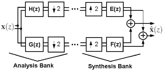
Figure 1: Two-channel multifilter bank.

In general, the design of the multifilter bank requires four multifilters: two on the analysis and two on the synthesis side. In perfect-reconstruction orthogonal MIMO filter banks, the analysis modulation matrix

$$M(z)=\begin{bmatrix}H(z)&H(-z)\\ G(z)&G(-z)\end{bmatrix}.$$

is paraunitary, that is

$$M^{*}(z)M(z)=M(z)M^{*}(z)=I.$$ (1)

In this case we can define the synthesis filters in terms of the analysis filters:

$$E(z)=H^{*}(z),\quad F(z)=G^{*}(z).$$

Eq. (1) can also be expressed as

$$\begin{split}H(z)H(z)^{*}+H(-z)H(-z)^{*}=I,\\ G(z)G(z)^{*}+G(-z)G(-z)^{*}=I,\\ H(z)G(z)^{*}+H(-z)G(-z)^{*}=0,\end{split}$$

or in terms of the coefficients

$$\begin{split}\sum_{k}C_{k}C_{k+2\ell}^{T}&=\sum_{k}D_{k}D_{k+2\ell}^{T}=\delta_{0\ell}\,I,\\ \sum_{k}C_{k}D_{k+2\ell}^{T}&=0,\end{split}$$

for any integer $\ell$.

Given $H(z)$, the matrix polynomial

$$P(z)=H(z)H^{*}(z)=\left(\sum_{k=0}^{n}C_{k}z^{-k}\right)\left(\sum_{k=0}^{n}C_{k}^{T}z^{k}\right)=\sum_{k=-n}^{n}P_{k}z^{k},$$

is called the matrix lowpass product filter (or scalar product filter in the case $r=1$). The coefficients $P_{k}$ satisfy $P_{-k}=P_{k}^{T}$. $P(z)$ is a half-band polynomial filter CNKS-96 , that is, it satisfies the equation

$$P(z)+P(-z)=2I.$$ (2)

This implies that $P_{0}=I$, and $P_{2\ell}=0$ for all nonzero integers $\ell$.

2.2 Multiwavelet Theory

2.2.1 Multiscaling and Multiwavelet Functions

Consider the iteration of a MIMO filter bank along the channel containing $H(z)$. After $k$ iterations, the equivalent filters will be

$$\begin{split}H^{(k)}(z)&=\prod_{j=0}^{k}H(z^{2^{j}})=H(z^{2^{k}})H(z^{2^{k-1}})\cdots H(z),\\ G^{(k)}(z)&=G(z^{2^{k}})\prod_{j=0}^{k-1}H(z^{2^{j}})=G(z^{2^{k}})H(z^{2^{k-1}})\cdots H(z),\end{split}$$

or in the time domain

$$C_{j}^{(k)} =\sum_{j}C_{j}^{(k-1)}C_{j-2^{k-1}}^{(k-1)},$$

$$D_{j}^{(k)} =\sum_{j}D_{j}^{(k-1)}D_{j-2^{k-1}}^{(k-1)},$$

where $C_{j}^{(0)}=C_{j}$, $D_{j}^{(0)}=D_{j}$.

The filterbank coefficients are associated with function vectors $\bm{\varphi}=[\phi_{0},\phi_{1},\ldots,\phi_{r-1}]^{T}$, called the multiscaling function, and $\bm{\psi}=[\psi_{0},\psi_{1},\ldots,\psi_{r-1}]^{T}$, called the multiwavelet function. These functions satisfy the recursion equations

$$\begin{split}\bm{\varphi}(t)&=\sqrt{2}\sum_{k=0}^{n}C_{k}\bm{\varphi}(2t-k),\\ \bm{\psi}(t)&=\sqrt{2}\sum_{k=0}^{n}D_{k}\bm{\varphi}(2t-k).\end{split}$$

The support of $\bm{\varphi}$, $\bm{\psi}$ is contained in the interval $[0,n]$, but it could be strictly smaller than the interval. See MRvF-96 for more details.

2.2.2 Multiwavelet Properties

Pre- and Postfiltering

Since multifilters are MIMO, they operate on several streams of input data rather than one. Therefore, input data needs to be vectorized. There are many prefilters available for various applications, but three kinds are preferred:

• Oversampling - Repeated Row Preprocessing

• Critical Sampling - Matrix Preprocessing

• Embedded Orthogonal Symmetric Prefilter Bank

In SW-00 , the first and second approach is presented for the GHM and CL multiwavelets. In practical applications, a popular choice is based on the Haar transform CMP-98 ; TST-99 . Haar pre- and postfilters have the advantage of simultaneously possessing symmetry and the orthogonality, and no multiplication is needed if one ignores the scaling factor. The problem of constructing symmetric prefilters is considered in detail in HSLS-03 , with proposed solutions for the DGHM and CL multifilters.

The third technique is applied in GM-05 ; HLSH-07 . They find a three-tap prefilter for the DGHM multifilter by searching among the parameters which minimize the first-order absolute moment of the filter coefficients.

Similarly, at the filter bank output, a postfilter is needed to reconstruct the signal. Pre- and postprocessing is not needed for scalar wavelets.

Balancing Order

The orthogonal multiscaling function is said to be balanced of order $q$ if the signals ${\mathbf{u}}_{k}=[\cdots,(-2)^{k},(-1)^{k},0^{k},1^{k},2^{k},\cdots]^{T}$ are preserved by the operator $L^{T}$ for $k=0,1,\ldots,q-1$. That is,

$$L^{T}{\mathbf{u}}_{k}=2^{-k}{\mathbf{u}}_{k},$$

where

$$L=\begin{bmatrix}\cdots\\ &C_{0}&C_{1}&\cdots&C_{n}\\ &&C_{0}&C_{1}&\cdots&C_{n}\\ &&&&&&\cdots\end{bmatrix}.$$

Multiwavelets that do not satisfy this property are said to be unbalanced. See LV-01 ; LV-98 ; PS-98 ; LP-11 for more details. Balanced multiwavelets do not require preprocessing.

Approximation Order

In the scalar case, a certain approximation order refers to the ability of the low-pass filter to reproduce discrete-time polynomials, while the wavelet annihilates discrete-time polynomials up to the same degree. Since many real-world signals can be modeled as polynomials, this property typically leads to higher coding gain (CG).

In the case of non-balanced multiwavelets, appropriate preprocessing is required to take advantage of approximation orders.

The approximation order of multiscaling and multiwavelet functions can be determined using the following result established in WLXL-10 . A multiscaling function provides approximation order $p$ iff there exist vectors ${\mathbf{u}}_{k}\in\,{\mathbb{R}}^{r}$, $0\leq k<p$, ${\mathbf{u}}_{0}\neq{\mathbf{0}}$, which satisfy

$$\begin{split}\sum_{\ell=0}^{k}\frac{1}{(2i)^{\ell}}\begin{pmatrix}k\\ \ell\end{pmatrix}{\mathbf{u}}_{k-\ell}^{T}D^{\ell}H(0)&=2^{-k}{\mathbf{u}}_{k}^{T},\\ \sum_{\ell=0}^{k}\frac{1}{(2i)^{\ell}}\begin{pmatrix}k\\ \ell\end{pmatrix}{\mathbf{u}}_{k-\ell}^{T}D^{\ell}H(\pi)&=0,\end{split}$$

where $D^{\ell}$ is the derivative of order $\ell$, and the masks of multiscaling and multiwavelet functions are

$$H(\omega)=\frac{1}{\sqrt{2}}\sum_{k=0}^{n}C_{k}e^{ik\omega},\qquad G(\omega)=\frac{1}{\sqrt{2}}\sum_{k=0}^{n}D_{k}e^{ik\omega}.$$ (3)

To fully characterize the multifilter bank with respect to approximation order we can add the condition

$$\sum_{\ell=0}^{k}\frac{1}{(2i)^{\ell}}\begin{pmatrix}k\\ \ell\end{pmatrix}{\mathbf{u}}_{k-\ell}^{T}D^{\ell}G(0)=0.$$

Good Multifilter Properties (GMPs)

A multiwavelet system can be represented by an equivalent scalar filter bank system TSLT-00 . The $r$ equivalent scalar filters are, in fact, the $r$ polyphases of the corresponding multifilter. This relationship motivates a new measure called good multifilter properties (GMPs) TSLT-98 , (TSLT-00, , (Def. 1)), which characterizes the magnitude response of the equivalent scalar filter bank associated with a multifilter. GMPs provide a set of design criteria imposed on the scalar filters, which can be translated directly to eigenvector properties of the designed multiwavelet filters.

An orthogonal multiwavelet system has GMPs of order at least $(1,1,1)$ if the following conditions are satisfied TSLT-00

$$\begin{split}{\mathbf{H}}(0){\mathbf{e}}(0)={\mathbf{e}}(0)\\ {\mathbf{H}}(r\pi){\mathbf{e}}(\pi)=0\\ {\mathbf{G}}(0){\mathbf{e}}(0)=0\end{split}$$

where $H(\omega)$ and $G(\omega)$ are masks of the lowpass and highpass filters (see eq. (3)), and

$${\mathbf{e}}(\omega)=[1,e^{-i\omega},e^{-2i\omega},\ldots,e^{-(r-1)i\omega}]^{T}.$$

A class of symmetric-antisymmetric biorthogonal multiwavelet filters which possess GMPs was introduced in TST-99 .

A GMP order of at least $(1,1,1)$ is critical for ensuring no frequency leakage across bands, hence improving compression performance. Multifilters possessing GMPs have better performance than those which do not possess GMPs LY-10 , due to better frequency responses for energy compaction, greater regularity and greater approximation order of the corresponding wavelet/scaling functions. GMPs help prevent both DC and high-frequency leakage across bands; this contributes to reduced smearing, blocking, ringing artifacts, and also helps to prevent checkerboard artifacts in reconstructed images for image coding.

The SA4 multiwavelet, introduced below in section 3.3, is a member of a one-parameter family of orthogonal multiwavelets with four coefficient matrices TSLT-00 . Different members of the family have different approximation order, but all of them have a GMP order of at least $(1,1,1)$. This manifests itself in the smooth decay to zero of the magnitude responses near $\omega=\pi$, compared to the following 4-tap orthogonal multiwavelet filters:

• The GHM multiwavelet DGHM-96 has symmetric orthogonal scaling functions and an approximation order of 2 for its filter length 4.

• Chui and Lian’s CL multiwavelet CL-96 has the highest possible approximation order of 3 for its filter length 3.

• Jiang’s multiwavelet JOPT4 J-98a has optimal time-frequency localization for its filter length.

Although the GHM and CL systems are the most commonly used orthogonal multiwavelet systems, and have higher approximation order than the SA4 system, they do not satisfy GMPs.

Smoothness

The smoothness of $\bm{\varphi}$, $\bm{\psi}$ can be characterized by Sobolev regularity $S$; this is discussed in MS-97 ; CDP-97 ; J-98b . The regularity estimate is related to both the eigenvalues and the corresponding eigenvectors of the transition operator and to spectral radius of the transition operator.

Symmetry and Antisymmetry

A function $g(t)$ is symmetric about a point $c$ if $g(c-t)=g(c+t)$ for all $t$. It is antisymmetric if $g(c-t)=-g(c+t)$.

For scaling functions and wavelets of compact support, the only possible symmetry is about the center of their support. For multiscaling and multiwavelet functions, this could be a different point for different components.

In the scalar case, the scaling function cannot be antisymmetric, since it must have a nonzero integral. In the multiwavelet case, some components even of $\bm{\varphi}$ can have antisymmetry.

2.3 Problem Statement

The design of perfect reconstruction multifilter banks and multiwavelets remains a significant problem. In the scalar case, spectral factorization of a half-band filter that is positive definite on the unit circle was, in fact, the first design technique, suggested by Smith and Barnwell SB-86 . This provides a motivation to extend the technique to the multiwavelet case. Spectral factorization of a Hermitian product filter in the multiwavelet case is more challenging than in the scalar case, and has not been investigated previously.

The present paper considers the application of MSF to the problem of finding an orthogonal lowpass multifilter $H(z)$, given a product filter $P(z)$. Since every orthogonal multiscaling filter $H(z)$ is a spectral factor of some matrix product filter, this can be used as a tool for designing new filters.

With an eye towards future applications, we are interested in constructing multifilters with desirable properties, especially GMPs. This implies that the determinant of $P(z)$ will have at least one zero of higher multiplicity on the complex unit circle. That is, $P(z)$ will be degenerate.

As a test case, we want to use a product filter $P(z)$ which satisfies the half-band condition (2), and is derived from an $H(z)$ which has more than 2 taps (i.e. $n\geq 3$) and good regularity properties and GMPs. Our benchmark test case will be the 2-channel orthogonal SA4 multiwavelet.

While there are many matrix spectral factorization algorithms CNKS-96 ; JK-85 ; L-93 , most cannot handle the degenerate case. We use Bauer’s method, based on the Toeplitz method of spectral factorization of the Youla and Kazanjian algorithm B-56 ; YK-78 , which can handle this case. However, convergence becomes very slow.

It is easy to see that matrix spectral factorization is not unique. If $H_{1}(z)$ is a factor of a given $P(z)$, then $H_{2}(z)=H_{1}(z)U$ is also a factor for any orthogonal matrix $U$, or more generally $H_{2}(z)=H_{1}(z)U(z)$ for paraunitary $U(z)$. Other operations may be permissible in some cases.

In our experiments with Bauer’s algorithm, the initial factors do not correspond to smooth functions. We apply regularization techniques, both to speed up convergence and to work towards recovering the original filter in this test case. In this manner, we derive two filters which we call the approximate and exact SA4 multiwavelets.

Let us briefly summarize some previous work.

Matrix Spectral Factorization (MSF) plays a crucial role in the solution of various applied problems for MIMO systems in communications and control engineering WMW-15 . It has been applied to designing minimum phase FIR filters and the associated all-pass filter HCW-10 , quadrature-mirror filter banks C-07 , MIMO systems for optimum transmission and reception filter matrices for precoding and equalization F-05 , precoders DXD-13 , and many other applications.

The analysis of linear systems corresponding to a given spectral density function was first established by Wiener, who used linear prediction theory of multi-dimensional stochastic processes WM-57 . The method of Wilson for MSF was developed for applications in the prediction theory of multivariate discrete time series, with known (or estimated) spectral density W-72 . Many numerical approaches to MSF have been proposed, for example CNKS-96 ; JK-85 ; L-93 . A survey of such algorithms is given in SK-01 ; however, this does not include algorithms for the degenerate case.

It is well known that all MSF methods have difficulties in this situation, and some of them cannot handle zeros on the unit circle at all. For example, Kučera’s algorithm, an otherwise popular matrix spectral factorization algorithm, has this limitation, and is not suitable for our purpose.

Bauer’s method was successful applied in LR-86 to the Radon projection. In that paper, factorization of the autocorrelation matrix of the Radon projection of a minimum phase pseudo-polynomial restored the coefficients of the original pseudo-polynomial with an accuracy around $10^{-17}$ after 10,000 recursions on a 64-bit floating point processor.

3 Matrix Spectral Factorization

The following theorem answers the existence question for MSF.

Theorem 3.1

(Matrix form of the Riesz-Fejér lemma HHS-04 ; EJL-09 ) A matrix polynomial

$$P(z)=\sum_{k=-n}^{n}P_{k}z^{k}$$

can be factored as $P(z)=H(z)H^{*}(z)$, where

$$H(z)=\sum_{k=0}^{n}C_{k}z^{-k}$$

is an $r$-channel causal polynomial matrix, if and only if $P(z)$ is symmetric positive semidefinite for $z$ on the complex unit circle.

3.1 Bauer’s Method

If $H(z)$ and $P(z)$ are known, we can construct doubly infinite block Toeplitz matrices $L$ and $T$ from their coefficients, by setting $L_{ij}=C_{i-j}$, $T_{ij}=T_{j-i}$. $T$ is symmetric and block banded with bandwidth $n$; $L$ is block lower triangular, also with bandwidth $n$.

The relation $P(z)=H(z)H^{*}(z)$ corresponds to $T=L\ L^{T}$, that is, $L$ is a Cholesky factor of $T$.

In Bauer’s method, we pick a large enough integer $f$, and truncate $T$ to (block) size $f\times f$:

$$T^{(f)}=\begin{pmatrix}P_{0}&P_{1}&\cdots&P_{n}&\\ P_{-1}&P_{0}&P_{1}&\cdots&P_{n}&\\ \vdots&&\ddots&&&\ddots&\\ P_{-n}&&&\ddots&&&P_{n}\\ &\ddots&&&\ddots&&\vdots\\ &&\ddots&&&\ddots&P_{1}\\ &&&P_{-n}&\cdots&P_{-1}&P_{0}\end{pmatrix}$$

If $T^{(f)}$ is positive definite, we can compute the Cholesky factorization $T=L^{(f)}\ L^{(f)T}$, where

$$L^{(f)}=\begin{pmatrix}C_{0}^{(1)}&\\ C_{1}^{(2)}&C_{0}^{(2)}&\\ \vdots&&\ddots&&&&\\ C_{n}^{(n+1)}&&&C_{0}^{(n+1)}&\\ &\ddots&&&\ddots&\\ &&C_{n}^{(f)}&\cdots&C_{1}^{(f)}&C_{0}^{(f)}\end{pmatrix}$$

It is shown in YK-78 that this factorization is possible, and that $C_{k}^{(f)}\to C_{k}$ as $f\to\infty$.

Bauer’s method works even in the case of highly degenerate $P(z)$. Unfortunately, convergence in this case is very slow.

3.2 Numerical Behavior

For chosen size $f$, the matrix $T^{(f)}$ is of size $2f\times 2f$. Its singular values are all in the range $[0,2]$. The first $(f-1)$ singular values are close to 2, then $\sigma_{f}=\sigma_{f+1}=1$, and the remaining $(f-1)$ singular values are close to 0. See fig. 2.

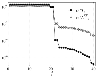
Figure 2: A sharp drop of the singular values of the Toeplitz matrix $T$ and of its spectral factor $L^{SF}$, for $f=20$; (filled circles) singular values of $T$; (hollow circles) singular values of $L^{SF}$.

The numerical stability of the factorization algorithm is good, until the higher singular values get too close to 0.

A bigger problem is the slow convergence. For example, in the scalar case $p(z)=z^{-1}+2+z$, where the factor is $h(z)=1+z^{-1}$, the value on the diagonal in row $f$ is

$$\sqrt{1+\frac{1}{f}}\approx 1+\frac{1}{2f},$$

which converges only very slowly to the limit 1. This simple problem has a double zero of the determinant on the unit circle. For higher order zeros, convergence speed becomes even worse.

3.3 Testing Bauer’s Method

A flowchart for testing Bauer’s method for MSF is shown in fig. 3. The steps are

• Choice of the benchmark multiscaling function $H(z)$;

• Construction of the matrix lowpass product filter $P(z)$;

• Find a spectral factor $L^{SF}=L^{(f)}$, and assess its quality;

• Do different kinds of postprocessing to obtain spectral factors $H^{(i)}$, $i=1,2,3$;

• Compare the obtained factors with the benchmark $H(z)$.

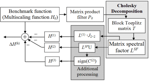
Figure 3: Steps in testing matrix spectral factorization using Bauer’s method.

Step 1: We consider the well-known orthogonal SA4 multiwavelet CL-96 ; HM-12 ; TSLT-00 as a benchmark testing case.

The recursion coefficients $C_{k}$ and $D_{k}$ of SA4 depend on a parameter $t$. They are

$$\begin{gathered}C_{0}=\alpha\begin{pmatrix}1&t\\ 1&-t\end{pmatrix};\quad C_{1}=\alpha\begin{pmatrix}t^{2}&t\\ -t^{2}&t\end{pmatrix};\quad C_{2}=\alpha\begin{pmatrix}t^{2}&-t\\ t^{2}&t\end{pmatrix};\quad C_{3}=\alpha\begin{pmatrix}1&-t\\ -1&-t\end{pmatrix};\\ D_{0}=\alpha\begin{pmatrix}t&-1\\ t&1\end{pmatrix};\quad D_{1}=\alpha\begin{pmatrix}-t&t^{2}\\ t&t^{2}\end{pmatrix};\quad D_{2}=\alpha\begin{pmatrix}-t&-t^{2}\\ -t&t^{2}\end{pmatrix};\quad D_{0}=\alpha\begin{pmatrix}t&1\\ -t&1\end{pmatrix};\end{gathered}$$ (4)

where $\alpha=1/(\sqrt{2}(1+t^{2}))$. In this paper, we use the filter with $t=4+\sqrt{15}$, which leads to $\alpha=(4-\sqrt{15})/(8\sqrt{2})$. Numerical values of $C_{k}$, $D_{k}$ are listed in table 1.

These coefficients generate the 2-band compactly supported orthogonal multiscaling function $\bm{\varphi}=[\phi_{0},\phi_{1}]^{T}$ and multiwavelet function $\bm{\psi}=[\psi_{0},\psi_{1}]^{T}$, all with support $[0,3]$. Graphs of these functions can be found in fig. 8 in a later chapter.

Table 1: Coefficients of the original SA4 multiscaling and multiwavelet functions.

$n$	$C_{n}$		$D_{n}$
$0$	$0.011226792152545$	$0.088388347648318$	$-0.088388347648318$	$0.011226792152545$
	$0.011226792152545$	$-0.088388347648318$	$-0.088388347648318$	$-0.011226792152545$
$1$	$0.695879989034003$	$0.088388347648318$	$0.088388347648318$	$-0.695879989034003$
	$-0.695879989034003$	$0.088388347648318$	$-0.088388347648318$	$-0.695879989034003$
$2$	$0.695879989034003$	$-0.088388347648318$	$0.088388347648318$	$0.695879989034003$
	$0.695879989034003$	$0.088388347648318$	$0.088388347648318$	$-0.695879989034003$
$3$	$0.011226792152545$	$-0.088388347648318$	$-0.088388347648318$	$-0.011226792152545$
	$-0.011226792152545$	$-0.088388347648318$	$0.088388347648318$	$-0.011226792152545$

Step 2: The symbol of the product lowpass multifilter $P$ has the form

$$P(z)=P_{3}^{T}z^{-3}+P_{1}^{T}z^{-1}+P_{0}+P_{1}z+P_{3}z^{3},$$

where

$$P_{0} =I,$$

$$P_{1}=P_{-1}^{T} =\frac{1}{64}\begin{pmatrix}4\sqrt{15}+17&&4\sqrt{15}+16\\ -4\sqrt{15}-16&&-4\sqrt{15}-17\end{pmatrix},$$

$$P_{2} =0,$$

$$P_{3}=P_{-3}^{T} =\frac{1}{64}\begin{pmatrix}15-4\sqrt{15}&&4\sqrt{15}-16\\ 16-4\sqrt{15}&&4\sqrt{15}-15\end{pmatrix}.$$

Numerical values of $P_{k}$ are given in table 2.

Table 2: The matrix coefficients $P_{k}$ of the half-band product filter $P$

$k$	$P_{k}$
0	1	0
	0	1
1	$0.507686459137964$	$0.492061459137964$
	$-0.492061459137964$	$-0.507686459137964$
3	$-0.007686459137964$	$-0.007938540862036$
	$0.007938540862036$	$0.007686459137964$

The impulse responses of the product filter (see fig. 4) have the character of nearly Haar-type scaling and wavelet functions. The frequency responses have good selectivity.

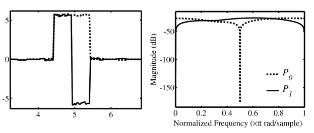
Figure 4: The impulse response (left) and frequency response (right) of the two components of the product filter $P=\left[P_{0};P_{1}\right]^{T}$.

Step 3: The matrix $T^{(f)}$ in this case looks like this:

$$T^{(f)}=\begin{pmatrix}P_{0}&P_{1}^{T}&0&P_{3}^{T}&\\ P_{1}&P_{0}&P_{1}^{T}&0&P_{3}^{T}&\\ 0&&\ddots&&&\ddots&\\ P_{3}&&&\ddots&&&P_{3}^{T}\\ &\ddots&&&\ddots&&0\\ &&\ddots&&&\ddots&P_{1}^{T}\\ &&&P_{3}&0&P_{1}&P_{0}\end{pmatrix}$$

For any fixed $f$, the coefficients from the last row of $L^{(f)}$ are approximate factors of $P(z)$. Suppressing the dependence on $f$ in the notation, we define the filter

$$L^{SF}(z)=\sum_{k=0}^{n}C_{k}^{(f)}z^{-k}$$

and the matrix

$$L^{SF} =\begin{bmatrix}C_{0}^{(f)}&C_{1}^{(f)}&C_{2}^{(f)}&C_{3}^{(f)}\end{bmatrix}$$ (5)

$$=\begin{bmatrix}L_{00}&L_{01}&L_{02}&L_{03}&L_{04}&L_{05}&L_{06}&L_{07}\\ L_{10}&L_{11}&L_{12}&L_{13}&L_{14}&L_{15}&L_{16}&L_{17}\end{bmatrix}.$$ (6)

This notation will be used again later.

To measure the quality of the factorization, we compute

$$\Delta P(z)=P(z)-L^{SF}(z)\ L^{SF*}(z)=\sum_{k=-n}^{n}\Delta P_{k}\ z^{k}.$$

The residual is then

$$\Delta P=\max_{k=-n,\ldots,n}\max_{ij}|(\Delta P_{k})_{ij}|.$$

In numerical experiments, the minimal error $\Delta P$ is achieved for $f=81$; the coefficients $C_{k}^{(81)}$ are given in table 3. The numerical error $\Delta P^{(81)}=3.169\cdot 10^{-9}$ for Bauer’s method is much better than that of Wilson’s method for MSF, which cannot be lower then $10^{-5}$ ESS-17 . The impulse response of the obtained spectral factor is non-regular, but the frequency response has good selectivity. This approximate factor does not quite provide perfect reconstruction. This is addressed in more detail in subsection 5.2.

Table 3: Coefficients of the lowpass spectral factor $L^{(f)}(z)$ for $f=81$, with $\Delta P^{(81)}=3.169\cdot 10^{-9}$.

$k$	$C_{k}^{(81)}$
$0$	0.094428373297668	0
	-0.091754813647953	0.022310801334572
$1$	0.175943193428843	0.679731045265413
	0.010360133828403	-0.702056243347588
$2$	0.000129414745433	0.700756678587017
	0.165030422671601	0.681046913905671
$3$	-0.081190837390599	0.021002135513698
	-0.083853536287580	-0.001275235049147

Steps 4 and 5 will be covered in chapter 4.

4 Construction of Approximate and Exact SA4 Multiwavelets

Above, we showed how to obtain the approximate spectral factor $L^{SF}$ for a given size $f$. Given any factor of $P$, other possible factors can be found be postmultiplication with suitable orthogonal matrices, or in some cases by other manipulations.

In subsection 4.1 we use a simple averaging process and column reversal to produce a lowpass filter that is similar to, but not identical to, the original SA4 multiscaling function. We call this the approximate SA4 multiwavelet.

In subsection 4.2, we add a rotation postfactor and an averaging process to produce another multiwavelet which is even closer to the original SA4 multiwavelet. We call this the exact SA4 multiwavelet.

The newly derived multiscaling filters are denoted by

$$H^{(1)}=\left[C_{0}^{(1)},C_{1}^{(1)},C_{2}^{(1)},C_{3}^{(1)}\right]$$

for the approximate SA4 multiwavelet, and

$$H^{(3)}=\left[C_{0}^{(3)},C_{1}^{(3)},C_{2}^{(3)},C_{3}^{(3)}\right]$$

for the exact SA4 multiwavelet. ($H^{(2)}$ is an intermediate step in the calculation of $H^{(3)}$). In each case, we find the corresponding multiwavelet filter by using a QR decomposition GvL-13 . The multiscaling filter is factorized as

$$\begin{pmatrix}C_{0}\\ C_{1}\\ C_{2}\\ C_{3}\end{pmatrix}=QR=\begin{pmatrix}|&&|\\ {\mathbf{q}}_{1}&\cdots&{\mathbf{q}}_{8}\\ |&&|\end{pmatrix}\cdot\begin{pmatrix}I\\ 0\\ 0\\ 0\end{pmatrix}$$

The coefficients $D_{k}$ are then obtained from the third and fourth columns of $Q$.

We define the absolute error by

$$\Delta H^{(k)}=H-H^{(k)}=\left[\Delta C_{0}^{(k)},\Delta C_{1}^{(k)},\Delta C_{2}^{(k)},\Delta C_{3}^{(k)}\right],$$

where $\Delta C_{n}^{(k)}=C_{n}-C_{n}^{(k)}$ for $k=1,2,3$, and likewise for $\Delta G^{(k)}$.

To measure the deviation of the new filters from the original, we introduce the mean square error (MSE) of the multiscaling and multiwavelet functions,

$$\mbox{MSE-MF}^{(k)}=\sum_{ij}|\Delta H_{ij}^{(k)}|^{2},\qquad\mbox{MSE-MwF}^{(k)}=\sum_{ij}|\Delta G_{ij}^{(k)}|^{2},$$

and themaximal absolute errors (MAE) of the matrix coefficients, the multiscaling function and the multiwavelet function as

$$\mbox{MAE-MC}_{\ell}^{(k)} =\max_{ij}|[\Delta C_{\ell}^{(k)}]_{ij}|,$$

MAE-MF $$=\max_{ij}|\Delta H_{ij}^{(k)}|=\max_{ij}|H_{ij}-H_{ij}^{(k)}|,$$

MAE-MwF $$=\max_{ij}|\Delta G_{ij}^{(k)}|=\max_{ij}|G_{ij}-G_{ij}^{(k)}|.$$

4.1 Approximate SA4 Multiwavelet

The spectral factor $L^{SF}$ obtained from Bauer’s method leads to non-symmetrical and non-regular functions. A simple algorithm can be used to symmetrize and regularize the scaling functions. Below, we are using the notation from eq. (5).

First, we average the absolute values of the first and fourth, as well as the second and third, matrix coefficients of the spectral factor:

$$\begin{split}L_{0,6}^{SF}&=\frac{1}{4}\left(|L_{00}^{SF}|+|L_{10}^{SF}|+|L_{06}^{SF}|+|L_{16}^{SF}|\right),\\ L_{1,7}^{SF}&=\frac{1}{4}\left(|L_{01}^{SF}|+|L_{11}^{SF}|+|L_{07}^{SF}|+|L_{17}^{SF}|\right),\\ L_{2,4}^{SF}&=\frac{1}{4}\left(|L_{02}^{SF}|+|L_{12}^{SF}|+|L_{04}^{SF}|+|L_{14}^{SF}|\right),\\ L_{3,5}^{SF}&=\frac{1}{4}\left(|L_{05}^{SF}|+|L_{15}^{SF}|+|L_{05}^{SF}|+|L_{15}^{SF}|\right).\end{split}$$

and construct average matrices

$$\begin{bmatrix}L_{2,4}^{SF}&L_{3,5}^{SF}\\ L_{2,4}^{SF}&L_{3,5}^{SF}\end{bmatrix},\qquad\begin{bmatrix}L_{0,6}^{SF}&L_{1,7}^{SF}\\ L_{0,6}^{SF}&L_{1,7}^{SF}\end{bmatrix}.$$

Second, the matrix coefficients $C_{1}^{(1)}$ and $C_{3}^{(1)}$ are obtained by multiplying the averaged matrices from the right by $J=\mbox{diag}(1,-1)$, but keep the signs, while the matrix coefficients $C_{0}^{(1)}$ and $C_{2}^{(1)}$ are obtained by multiplying $C_{1}^{(1)}$ and $C_{3}^{(1)}$ on the left and right by $U=\mbox{antidiag}(1,1)$:

$$\begin{split}C_{3}^{(1)}&=\mbox{sign}(L_{3}^{SF})\begin{bmatrix}L_{0,6}^{SF}&L_{1,7}^{SF}\\ L_{0,6}^{SF}&L_{1,7}^{SF}\end{bmatrix}\cdot J,\\ C_{0}^{(1)}&=U\cdot C_{3}^{(1)}\cdot U,\\ C_{1}^{(1)}&=\mbox{sign}(L_{1}^{SF})\begin{bmatrix}L_{2,4}^{SF}&L_{3,5}^{SF}\\ L_{2,4}^{SF}&L_{3,5}^{SF}\end{bmatrix}\cdot J,\\ C_{2}^{(1)}&=U\cdot C_{1}^{(1)}\cdot U.\end{split}$$

This produces coefficients quite close to the original coefficients in (4).

In order to determine the best approximate solution, we investigate the influence of the size $f$ of the Toeplitz matrix $T^{(f)}$ for the numerical errors MAE-MF⁽¹⁾, MSE-MC${}_{0}^{(1)}$, and MSE-MC${}_{1}^{(1)}$. These errors are shown in fig. 5 in logarithmic scale, for $f$ up to 100. Note that MSE-MC${}_{3}^{(1)}$ = MSE-MC${}_{0}^{(1)}$, and MSE-MC${}_{2}^{(1)}$ = MSE-MC${}_{1}^{(1)}$, by construction.

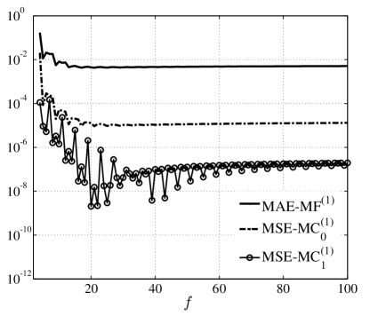
Figure 5: Dependence of maximum absolute error MAE-MF⁽¹⁾ and mean squared errors MSE-MC${}_{0}^{(1)}$ = MSE-MC${}_{3}^{(1)}$, MSE-MC${}_{1}^{(1)}$ = MSE-MC${}_{2}^{(1)}$ on matrix size $f$ (log. scale).

The important minimal errors MAE-MF⁽¹⁾ and MSE-MwF⁽¹⁾ for $f=21$ are tabulated in table 4; the matrix coefficients of are listed in table 5. Obviously, the development of the errors shows the convergence of the algorithm, as well as the dependency of the errors on the size $f$. It also shows that the main error comes from the matrix coefficients $C_{0}^{(1)}$ and $C_{3}^{(1)}$, rather than $C_{1}^{(1)}$ and $C_{2}^{(1)}$.

The error MSE-MF⁽¹⁾ behaves essentially the same way as MAE-MC${}_{0}^{(1)}$. Unfortunately, the convergence of MAE-MC${}_{0}^{(1)}$ and MAE-MC${}_{3}^{(1)}$ stalls at a relatively large number. Thus, the approximate SA4 multiwavelet is not very accurate. Better matrix coefficients are achieved in the next subchapter.

Table 4: The minimum MAEs and MSEs for the approximate and exact SA4 multiscaling and multiwavelet functions, the size $f$ and the corresponding angle $\theta$.

$f$		MAE-MF(1)	MAE-MwF(1)	MSE-MF(1)	MSE-MwF(1)
21		$4.2797\cdot 10^{-3}$		$4.6139\cdot 10^{-6}$
$f$	$\theta$	MAE-MF(2)	MAE-MwF(2)	MSE-MF(2)	MSE-MwF(2)
15,400	$1.444628609880879$	$1.220\cdot 10^{-4}$		$7.376\cdot 10^{-9}$
$f$	$\theta$	MAE-MF(3)	MAE-MwF(3)	MSE-MF(3)	MSE-MwF(3)
12,042	$1.444630025395427$	$8.285\cdot 10^{-8}$	$8.557\cdot 10^{-8}$	$3.835\cdot 10^{-15}$	$3.717\cdot 10^{-15}$

Table 5: Coefficients of the approximate SA4 multiscaling and multiwavelet functions for $f=21$.

n	$C_{n}^{(3)}$		$D_{n}^{(3)}$
$0$	$0.011165766264837$	$0.088552225597447$	$-0.088552225597447$	$0.011165766264837$
	$0.011165766264837$	$-0.088552225597447$	$-0.088552225597447$	$-0.011165766264837$
$1$	$0.691600252880066$	$0.088718768987217$	$0.088718768987217$	$-0.691600252880066$
	$-0.691600252880066$	$0.088718768987217$	$-0.088718768987217$	$-0.691600252880066$
$2$	$0.691600252880066$	$-0.088718768987217$	$0.088718768987217$	$0.691600252880066$
	$0.691600252880066$	$0.088718768987217$	$0.088718768987217$	$-0.691600252880066$
$3$	$0.011165766264837$	$-0.088552225597447$	$-0.088552225597447$	$-0.011165766264837$
	$-0.011165766264837$	$-0.088552225597447$	$0.088552225597447$	$-0.011165766264837$

4.2 Exact SA4 Multiwavelet

The second algorithm leads to more regular scaling functions. We multiply the coefficients of $L^{SF}$ from the right by the unitary matrix $U(\theta)$

$$C_{k}^{(2)}=C_{k}^{SF}\cdot U(\theta)=C_{k}^{SF}\cdot\begin{pmatrix}\cos\theta&\sin\theta\\ -\sin\theta&\cos\theta\end{pmatrix},\qquad k=0,\ldots,3.$$

This produces the approximate factor $H^{(2)}$.

The angle $\theta$ (in radians) is calculated as the average value

$$\theta=\frac{1}{2}\left(\cos^{-1}(\mbox{even})+\sin^{-1}(\mbox{odd})\right),$$

where

$$\mbox{even}=\frac{1}{4}\left(\left|L_{00}+L_{04}+L_{10}+L_{14}\right|+\left|L_{02}+L_{06}+L_{12}+L_{16}\right|\right)$$

and

$$\mbox{odd}=\frac{1}{4}\left(\left|L_{01}+L_{05}+L_{11}+L_{15}\right|+\left|L_{03}+L_{07}+L_{13}+L_{17}\right|\right).$$

Again, we are using the notation from eq. (5).

Figure 6 shows the dependence of the angle $\theta$ on the size $f$ (log. scale). It can be seen that in the angle there is one overshoot, after that it is decreasing very slowly. The minimum errors are obtained at the maximal possible size of Toeplitz matrix $f=15,400$, with the values shown in table 4. This shows the influence of the very slow convergence; despite right multiplication with the unitary matrix, desirable precison cannot be an achieved. The errors MSE-MF⁽²⁾ and MAE-MF⁽²⁾ for $H^{(2)}$ are shown in fig. 7.

To increase the numerical precision and obtain the exact SA4 multiscaling function, we again apply an averaging approach.

$$H^{(3)} =[C_{0}^{(3)},C_{1}^{(3)},C_{2}^{(3)},C_{3}^{(3)}],$$

$$(C_{0}^{(3)})_{ij} =\mbox{sign}((C_{0}^{(2)})_{ij})\cdot\frac{1}{2}\left(\left|(C_{0}^{(2)})_{ij}\right|+\left|(C_{3}^{(2)})_{ij}\right|\right),$$

$$(C_{1}^{(3)})_{ij} =\mbox{sign}((C_{1}^{(2)})_{ij})\cdot\frac{1}{2}\left(\left|(C_{1}^{(2)})_{ij}\right|+\left|(C_{2}^{(2)})_{ij}\right|\right),$$

$$(C_{2}^{(3)})_{ij} =\mbox{sign}((C_{2}^{(2)})_{ij})\cdot\frac{1}{2}\left(\left|(C_{1}^{(2)})_{ij}\right|+\left|(C_{2}^{(2)})_{ij}\right|\right),$$

$$(C_{3}^{(3)})_{ij} =\mbox{sign}((C_{3}^{(2)})_{ij})\cdot\frac{1}{2}\left(\left|(C_{0}^{(2)})_{ij}\right|+\left|(C_{3}^{(2)})_{ij}\right|\right).$$

The errors for $H^{(3)}$ are shown in fig. 7, with minima shown in table 4. Let us consider the accuracy of the multiscaling functions obtained at the leading local minima of the error MAE-MF⁽³⁾ . There are 3 minima, as can be seen in the zoomed part of fig. 7. The first local minimum is at the value $f=4,269$, the second at $f=9,139$, the third at $f=12,042$. This means that increasing the size of the Toeplitz matrix leads to slow improvement in the precision of the exact multiscaling function. Nevertheless, due to applying the averaging method, the minimal errors in $H^{(3)}$ and $G^{(3)}$ for $f=12,042$ are smaller by 2 or 3 orders of magnitude than the errors in $H^{(2)}$ and $G^{(2)}$, and smaller by 5 orders of magnitude than the errors in $H^{(1)}$ and $G^{(1)}$.

We choose $H^{(3)}$ for $f=12,042$ for the coefficients of the exact SA4 multiwavelet, given in table 6. They are almost the same as the original coefficients in (4).

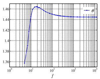
Figure 6: Dependence of the angle $\theta$ (radians) on size $f$ (log scale).

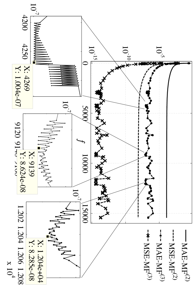
Figure 7: Dependence of the errors MSE-MF⁽ⁱ⁾ and MAE-MF⁽ⁱ⁾ $i=2,3$, on the size of $f$ (log scale).

Table 6: Coefficients of the exact SA4 multiscaling and multiwavelet functions for $f=12,042$.

n	$C_{n}^{(3)}$		$D_{n}^{(3)}$
$0$	$0.01122679201336641$	$0.08838843031594616$	$-0.08838843285624247$	$0.01122679262734716$
	$0.01122679228175923$	$-0.08838843013543155$	$-0.08838843302944295$	$-0.01122679235802515$
$1$	$0.6958799459541121$	$0.08838843050191729$	$0.08838843089794699$	$-0.6958799676294173$
	$-0.6958799462085388$	$0.08838842817713602$	$-0.08838843321541406$	$-0.6958799673174058$
$2$	$0.6958799459541121$	$-0.08838843050191729$	$0.08838843089794699$	$0.6958799676294172$
	$0.6958799462085388$	$0.08838842817713602$	$0.08838843321541406$	$-0.6958799673174058$
$3$	$0.01122679201336641$	$-0.08838843031594616$	$-0.08838843285624255$	$-0.01122679262734722$
	$-0.01122679228175923$	$-0.08838843013543155$	$0.08838843302944295$	$-0.01122679235802536$

5 Performance Analysis

5.1 Comparison With Other Multiwavelets

Table 7 gives the results of our experiments with the approximate and exact SA4 multiwavelets, compared with other well-known orthogonal and biorthogonal filter banks. Comparisons include coding gain (CG), Sobolev smoothness (S) CMP-98 , symmetry/antisymmetry, and length. All of the multiwavelets considered have symmetry/antisymmetry.

The CG for orthogonal transforms is a good indication of the performance in signal processing. It is the ratio of arithmetic and geometric means of channel variances $\sigma_{i}^{2}$:

$$CG=\frac{\frac{1}{r}\sum_{i=1}^{r}\sigma_{i}^{2}}{\left(\prod_{i=1}^{r}\sigma_{i}^{2}\right)^{1/r}}$$

Coding gain is one of the most important factors to be considered in many applications. It is always greater than or equal to 1; greater values are better. CG is equal to 1 if all the variances are equal, which means that it is not possible to clearly distinguish between the smooth and the detailed components of the multiwavelet transformation coefficients. To estimate CG, the variance is computed using a first order Markov model AR(1) with intersample autocorrelation coefficient $\rho=0.95$ DS-98 .

The Sobolev exponent $S$ of a filter bank measures the $L^{2}$-differentiability of the corresponding multiscaling function $\bm{\varphi}=[\phi_{0},\phi_{1}]^{T}$, and thus also the multiwavelet function $\bm{\psi}=[\psi_{0},\psi_{1}]^{T}$. It is completely determined by the multiscaling symbol $H(z)$.

The obtained Sobolev regularity and CGs of the approximate and exact SA4 multiwavelets are equal: $S^{(1)}=S^{(3)}=0.9919$, and $CG^{(1)}=CG^{(3)}=3.7323$ dB. This means that for some applications we can use the SA4 multiwavelet.

According to table 7, the approximate and exact SA4 multiwavelets are better than most commonly used filter banks. They also allow an economical lifting scheme for future implementation.

Fig. 8 shows a comparison of the approximate and exact SA4 multiwavelets in time domain and impulse response. The influence of the lower precision of the approximate SA4 multiwavelet can be seen in the time domain image.

Table 7: Comparison of coding gain (CG), Sobolev regularity (S), symmetry/antisymmetry (S/A), and length, for various multiwavelets.

Multifilter	CG	S	S/A	Length
Biorthogonal Hermitian cubic spline (bih34n, S-98 )	1.51	2.5	yes	3/5
Biorthogonal (dual to Hermitian cubic spline) (bih32s, AZC-07 )	1.01	2.5	yes	3/5
Integer Haar CP-01	1.83	0.5	yes	2
Chui-Lian (CL, CL-96 )	2.06	1.06	yes	3
Biorthogonal (dual to Hermitian cubic spline) (bih54n, AZC-07 )	2.42	0.61	yes	5/3
Biorthogonal (from GHM) (bighm2, AZC-07 )	2.43	0.5	yes	2/6
Biorthogonal (from GHM, dual to bighm2) (bighm6, AZC-07 )	3.53	2.5	yes	6/2
Biorthogonal (dual to Hermitian cubic spline) (bih52s, T-98 )	3.69	0.83	yes	5/3
Approximate SA4	3.73	0.99	yes	4
Exact SA4 (STT-00 )	3.73	0.99	yes	4
Geronimo-Hardin-Massopust (GHM, GHM-94 )	4.41	1.5	yes	4

The magnitude of the approximate SA4 in the time domain is observably smaller than for the exact SA4, while the frequency responses are essentially identical (see fig. 8). Therefore, in applications where the frequency response is important, we can use the approximate multiscaling function.

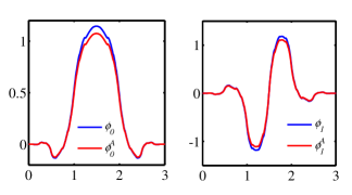
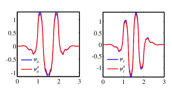
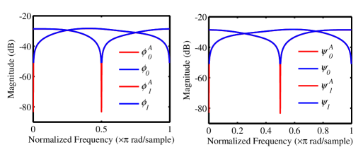
Figure 8: Top: The impulse responses of the components of the exact SA4 multiwavelet $\bm{\varphi}=(\phi_{0},\phi_{1})^{T}$, $\bm{\psi}=(\psi_{0},\psi_{1})^{T}$ (in blue), compared with the approximate multiwavelet $\bm{\varphi}^{A}=(\phi_{0}^{A},\phi_{1}^{A})^{T}$, $\bm{\psi}^{A}=(\psi_{0}^{A},\psi_{1}^{A})^{T}$ (in red); left to right: $\phi_{0}$, $\phi_{1}$, $\psi_{0}$, $\psi_{1}$; Bottom: The frequency response of the components of the exact SA4 multiwavelet (in blue) compared with the approximate multiwavelet (in red); left: $\phi_{0}$, $\phi_{1}$; right: $\psi_{0}$, $\psi_{1}$.

5.2 Influence of Inaccuracy of Filter Coefficients with Approximate SA4 Multiwavelet

The approximate SA4 multiwavelet $H^{(1)}$ is not quite an orthogonal perfect reconstruction filter. In this section, we explore whether it can still be useful in applications.

5.2.1 1D Signal (No Additional Processing)

The influence of the inaccuracy of the matrix filter coefficients in the case of the approximate SA4 multiwavelet is shown by 1D applications with no additional processing. By “no additional processing” we mean that we simply decompose and reconstruct a signal through several levels. No compression, denoising, or other processing is done.

We use Haar balancing pre- and postfilters CMP-98 ; SHSTH-99

$$Q=\frac{1}{\sqrt{2}}\begin{pmatrix}1&1\\ -1&1\end{pmatrix},$$

whose small length preserves the time localization of the multiwavelet decomposition, simplicity, orthogonality, and symmetry.

Results for the balanced version are shown in fig. 9(b).

The error in orthogonality of the approximate balanced SA4 multiwavelet is

$$\Delta H=I-Q\cdot H^{(1)}\cdot(H^{(1)})^{T}Q^{T}=0.0117\ I.$$

For the quality measure, we decompose and reconstruct five normed test signals of length $N=2^{7}$, $s$ (without noise) and $\hat{s}=s+\epsilon$ (with noise). The number of decomposition levels is 6.

The noise components $\epsilon_{i}$ are independent identically distributed random variables with mean 0 and standard deviation $\sigma$. We use maximum absolute errors (MAE)

$$\Delta s=\max_{i}\left|\mbox{reconstructed }s_{i}-\mbox{original }s_{i}\right|,$$

where $s_{i}$ refers to the $i^{\mbox{\scriptsize th}}$ test signal.

The test signals are ’Cusp’, ’HiSine’, ’LoSine’, ’Piece-regular’, and ’Piece-polynomial’, implemented in the Matlab environment. See fig. 9(a).

(a)
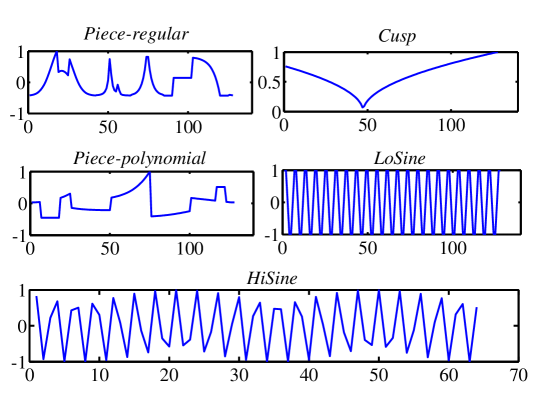
(b)

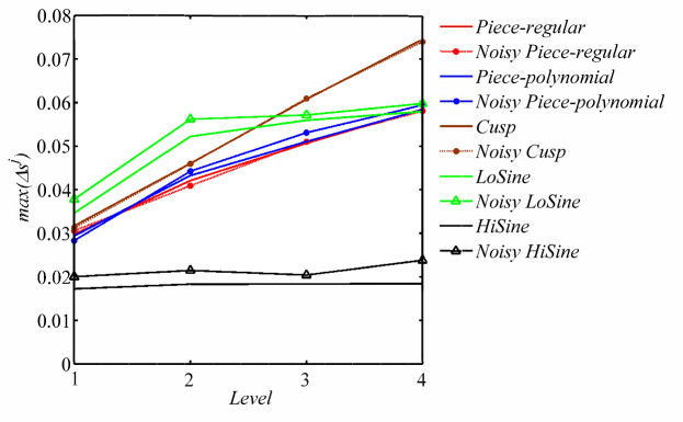
Figure 9: Decomposition and reconstruction with the balanced approximate SA4 multiwavelet; (a) The normed test signals; (b) The MAEs obtained at level $j$.

For the test signal ’Cusp’, increasing the number of decomposition and reconstruction levels $j$ leads to a linear increase of MAE. From the obtained small differences (about $3.5\cdot 10^{-4}$) in error between noisy and noiseless signal, it follows that the presence of noise does not make much difference in signals of this type.

For the test signal ’HiSine’ we observe nearly constant MAEs for the noisy and noiseless signals with increasing level $j$; the difference between the noisy and noiseless signal is in the interval $[2-5.3]\cdot 10^{-3}$. Again, the presence of noise has only a minimal influence.

For the test signal ’LoSine’, both noisy and noiseless MAEs show a linear increase up to the second level, with only a small increase at the third and fourth level of $-5.7\cdot 10^{-3}$ and $3.6\cdot 10^{-3}$, as shown in fig. 9(b). Therefore, after the second level the influence of noise is weak.

For the test signal ’Piece-regular’, the MAE grows quadratically with increasing $j$. The difference between noisy and noiseless signals is smallest at a pre-/post-processing step ($6\cdot 10^{-5}$ and largest at the second level ($1.2\cdot 10^{-3}$). For the test signal ’Piece-polynomial’, the MAE grows non-uniformly and non-linearly with increasing $j$. The difference between noisy and noiseless signals is smallest at the pre-/post-processing step ($3.8\cdot 10^{-4}$) and largest at the third level ($2\cdot 10^{-3}$).

5.2.2 2D Signal (No Additional Processing)

The performance of the approximate SA4 multiwavelet was tested by decomposing and reconstructing several gray level images, through 6 or 7 levels. Fig. 10 shows the details for four of the images, with the quality measure $PSNR=\log_{10}(255^{2}/MSE)$ dB. The images used are ’Lena’ , ’Peppers’, ’Girlface’, and ’Barbara’.

The approximate balanced SA4 multiwavelet applied to the four images leads to an exponential decrease of the PSNRs. According to these results, it is preferable to use no more than 3 or 4 levels of decomposition. After that, the reconstructed image has very low PSNRs and visibly worse quality. In some applications, such as big data archives, higher levels of decomposition may be useful.

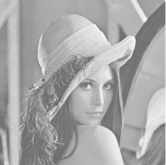
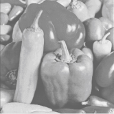
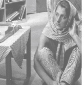
(a) (b) (c)
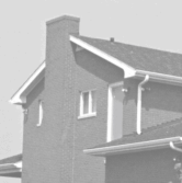
(d) (e) (f)

Figure 10: Test images of size $256\times 256$ pixels) (a) Lena, (b) Peppers, and ($512\times 512$ pixels) (c) House, (d) Girlface, (e) Barbara, and (f) Zelda.

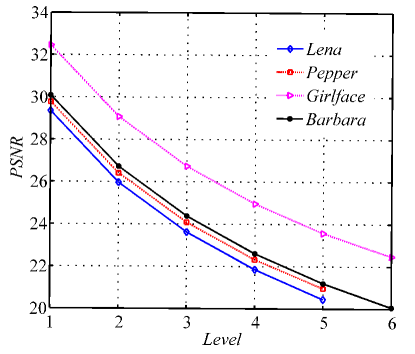
Figure 11: The PSNRs of four images for 2D decomposition and reconstruction without additional processing of 1 through 6 or 7 levels with the approximate SA4 multiwavelet.

5.3 Image Denoising

In this section, we compare the balanced and non-balanced version of the exact SA4 multiwavelet with the GHM multiwavelet (Downie and Silverman 1998) and the Chui-Lian multiwavelet CL (Downie and Silverman 1998), by considering image denoising with vector hard thresholding (Donoho and Johnstone 1994), using 1-5 levels. The images are ’Lena’, ’Zelda’, and ’House’, of size $512\times 512$ pixels, with white additive Gaussian noise with variance $\sigma=10$. See fig. 10.

The multiwavelet coefficients of the white noise are reduced at each level, but uniformly distributed within each level. Therefore, the best approach to denoising is to find an appropriate threshold value at each level.

The exact SA4 multiwavelet, both balanced and non-balanced, achieved the maximal PSNRs. The PSNR differences for the both versions of the test images are $3.57$ dB at the pre-/post-processing step and $4.06$ dB at the fifth level for “Lena”; $4.17$ dB (pre-/post-processing step) and $5.13$ dB (fifth level) for “Zelda”, $5.09$ dB (pre-/post-processing step) and $6.53$ dB (fifth level) for House”. Although balancing of multiwavelets destroys the symmetry, it leads to increasing PSNRs and better image denoising with the exact SA4 multiwavelet for the three test images for the both version multiwavelets, while for the non-balanced GHM and CL multiwavelets PSNRs decrease (see fig. 12(a)).

According to PSNRs, image decomposition and reconstruction through two levels with the approximate SA4 multiwavelet is comparable to image denoising with the non-balanced SA4 multiwavelet through three levels, while one level is comparable with the balanced multiwavelet pre-/post-processing step (see fig. 11 and fig. 12).

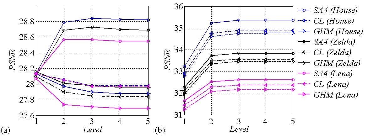
Figure 12: Comparative analysis of PSNRs for image denoising with the exact SA4 multiwavelet and vector hard threshold through 2-6 levels of the images ’House’, ’Zelda’, and ’Lena’ with $512\times 512$ pixels and white additive Gaussian noise with variance $\sigma=10$. Left: Non-balanced multiwavelets; Right: Balanced multiwavelets.

Obviously, the PSNRs of the exact balanced SA4 multiwavelet are better than the well-known orthogonal multiwavelets GHM and CL. They are useful in many applications.

6 Conclusion

In this paper, we consider for the first time the problem of obtaining an orthogonal multiscaling function by matrix spectral factorization from a degenerate polynomial matrix. We show benchmark testing of MSF, and apply Bauer’s method to factoring the product filter of the SA4 multiwavelet. In addition, we show how to remove numerical errors and improve the properties of the factors obtained from Cholesky factorization, leading to fast convergent algorithms.

A very important part is obtaining the key angle $\theta$ in explicit form. Based on the proposed averaging approach, we develop two filter banks, the approximate and the exact SA4 orthogonal multiwavelets.

Experimental results have shown that the performances of the resulting multiwavelets are better than those of the Chui-Lian multiwavelet and biorthogonal multifilters, and are highly comparable to that of longer multiwavelets. Theoretical analyses for the influence of the size $f$ of the Toeplitz matrix are considered, as well as simple 1D and 2D applications.

After comparing both types of multifilters, we concluded that the proposed averaging approach is a better way to remove numerical errors and find the exact SA4 multiwavelet filter bank. It is important to note that the performance of the balanced exact SA4 multiwavelet for image denoising is better than the well-known orthogonal multiwavelets GHM and CL, which are longer.

- (1) Averbuch, A.Z., Zheludev, V.A., Cohen, T.: Multiwavelet frames in signal space originated from Hermite splines. IEEE Trans. Signal Process. 55(3), 797–808 (2007)
- (2) Bauer, F.L.: Beiträge zur Entwicklung numerischer Verfahren für programmgesteuerte Rechenanlagen. II. Direkte Faktorisierung eines Polynoms. Bayer. Akad. Wiss. Math.-Nat. Kl. S.-B. 1956, 163–203 (1957) (1956)
- (3) Charoenlarpnopparut, C.: One-dimensional and multidimensional spectral factorization using gröbner basis approach. In: 2007 Asia-Pacific Conference on Communications, pp. 201–204 (2007)
- (4) Cheung, K.W., Po, L.M.: Integer multiwavelet transform for lossless image coding. In: Intelligent Multimedia, Video and Speech Processing, 2001. Proceedings of 2001 International Symposium on, pp. 117–120 (2001)
- (5) Chui, C.K., Lian, J.A.: A study of orthonormal multi-wavelets. Appl. Numer. Math. 20(3), 273–298 (1996). Selected keynote papers presented at 14th IMACS World Congress (Atlanta, GA, 1994)
- (6) Cohen, A., Daubechies, I., Plonka, G.: Regularity of refinable function vectors. J. Fourier Anal. Appl. 3(3), 295–324 (1997)
- (7) Cooklev, T., Nishihara, A., Kato, M., Sablatash, M.: Two-channel multifilter banks and multiwavelets. In: Conference Proceedings, IEEE International Conference on Acoustics, Speech, and Signal Processing ICASSP-96, vol. 5, pp. 2769–2772 (1996)
- (8) Cotronei, M., Montefusco, L.B., Puccio, L.: Multiwavelet analysis and signal processing. IEEE Transactions on Circuits and Systems II: Analog and Digital Signal Processing 45(8), 970–987 (1998)
- (9) Donoho, D.L., Johnstone, I.M.: Ideal spatial adaptation by wavelet shrinkage. Biometrika 81(3), 425–455 (1994)
- (10) Donovan, G.C., Geronimo, J.S., Hardin, D.P., Massopust, P.R.: Construction of orthogonal wavelets using fractal interpolation functions. SIAM J. Math. Anal. 27(4), 1158–1192 (1996)
- (11) Downie, T.R., Silverman, B.W.: The discrete multiple wavelet transform and thresholding methods. IEEE Transactions on Signal Processing 46(9), 2558–2561 (1998)
- (12) Du, B., Xu, X., Dai, X.: Minimum-phase FIR precoder design for multicasting over MIMO frequency-selective channels. Journal of Electronics (China) 30(4), 319–327 (2013)
- (13) Ephremidze, L., Janashia, G., Lagvilava, E.: A simple proof of the matrix-valued Fejér-Riesz theorem. Journal of Fourier Analysis and Applications 15(1), 124–127 (2009)
- (14) Ephremidze, L., Saied, F., Spitkovsky, I.: On the algorithmization of Janashia-Lagvilava matrix spectral factorization method. Submitted to IEEE Trans. Inform. Theory
- (15) Fischer, R.F.: Sorted spectral factorization of matrix polynomials in MIMO communications. IEEE Transactions on Communications 53(6), 945–951 (2005)
- (16) Gan, L., Ma, K.K.: On minimal lattice factorizations of symmetric-antisymmetric multifilterbanks. IEEE Trans. Signal Process. 53(2, part 1), 606–621 (2005)
- (17) Geronimo, J.S., Hardin, D.P., Massopust, P.R.: Fractal functions and wavelet expansions based on several scaling functions. J. Approx. Theory 78(3), 373–401 (1994)
- (18) Golub, G.H., Van Loan, C.F.: Matrix computations, fourth edn. Johns Hopkins Studies in the Mathematical Sciences. Johns Hopkins University Press, Baltimore, MD (2013)
- (19) Hansen, M., Christensen, L.P.B., Winther, O.: Computing the minimum-phase filter using the QL-factorization. IEEE Trans. Signal Process. 58(6), 3195–3205 (2010)
- (20) Hardin, D.P., Hogan, T.A., Sun, Q.: The matrix-valued Riesz lemma and local orthonormal bases in shift-invariant spaces. Advances in Computational Mathematics 20(4), 367–384 (2004)
- (21) Hsung, T.C., Lun, D.P.K., Shum, Y.H., Ho, K.C.: Generalized discrete multiwavelet transform with embedded orthogonal symmetric prefilter bank. IEEE Trans. Signal Process. 55(12), 5619–5629 (2007)
- (22) Hsung, T.C., Sun, M.C., Lun, D.K., Siu, W.C.: Symmetric prefilters for multiwavelets. IEE Proceedings-Vision, Image and Signal Processing 150(1), 59–68 (2003)
- (23) Huo, G., Miao, L.: Cycle-slip detection of GPS carrier phase with methodology of SA4 multi-wavelet transform. Chinese Journal of Aeronautics 25(2), 227–235 (2012)
- (24) Ježek, J., Kučera, V.: Efficient algorithm for matrix spectral factorization. Automatica 21(6), 663–669 (1985)
- (25) Jiang, Q.: On the regularity of matrix refinable functions. SIAM J. Math. Anal. 29(5), 1157–1176 (1998)
- (26) Jiang, Q.: Orthogonal multiwavelets with optimum time-frequency resolution. IEEE Trans. Signal Process. 46(4), 830–844 (1998)
- (27) Lawton, W.: Applications of complex valued wavelet transforms to subband decomposition. IEEE Transactions on Signal Processing 41(12), 3566–3568 (1993)
- (28) Lebrun, J., Vetterli, M.: Balanced multiwavelets theory and design. IEEE Trans. Signal Process. 46(4), 1119–1125 (1998)
- (29) Lebrun, J., Vetterli, M.: High-order balanced multiwavelets: theory, factorization, and design. IEEE Trans. Signal Process. 49(9), 1918–1930 (2001)
- (30) Li, B., Peng, L.: Balanced multiwavelets with interpolatory property. IEEE Trans. Image Process. 20(5), 1450–1457 (2011)
- (31) Li, Y.F., Yang, S.Z.: Construction of paraunitary symmetric matrices and parametrization of symmetric orthogonal multiwavelet filter banks. Acta Math. Sinica (Chin. Ser.) 53(2), 279–290 (2010)
- (32) Massopust, P.R., Ruch, D.K., Van Fleet, P.J.: On the support properties of scaling vectors. Appl. Comput. Harmon. Anal. 3(3), 229–238 (1996)
- (33) Micchelli, C.A., Sauer, T.: Regularity of multiwavelets. Adv. Comput. Math. 7(4), 455–545 (1997)
- (34) Plonka, G., Strela, V.: Construction of multiscaling functions with approximation and symmetry. SIAM J. Math. Anal. 29(2), 481–510 (1998)
- (35) Roux, J.L.: 2D spectral factorization and stability test for 2D matrix polynomials based on the radon projection. In: Acoustics, Speech, and Signal Processing, IEEE International Conference on ICASSP ’86., vol. 11, pp. 1041–1044 (1986)
- (36) Sayed, A.H., Kailath, T.: A survey of spectral factorization methods. Numer. Linear Algebra Appl. 8(6-7), 467–496 (2001). Numerical linear algebra techniques for control and signal processing
- (37) Shen, L., Tan, H.H., Tham, J.Y.: Symmetric-antisymmetric orthonormal multiwavelets and related scalar wavelets. Appl. Comput. Harmon. Anal. 8(3), 258–279 (2000)
- (38) Smith, M., Barnwell, T.: Exact reconstruction techniques for tree-structured subband coders. IEEE Transactions on Acoustics, Speech, and Signal Processing 34(3), 434–441 (1986)
- (39) Strela, V.: A note on construction of biorthogonal multi-scaling functions. In: Wavelets, multiwavelets, and their applications (San Diego, CA, 1997), Contemp. Math., vol. 216, pp. 149–157. Amer. Math. Soc., Providence, RI (1998)
- (40) Strela, V., Heller, P.N., Strang, G., Topiwala, P., Heil, C.: The application of multiwavelet filterbanks to image processing. IEEE Transactions on Image Processing 8(4), 548–563 (1999)
- (41) Strela, V., Walden, A.: Signal and image denoising via wavelet thresholding: orthogonal and biorthogonal, scalar and multiple wavelet transforms. In: Nonlinear and nonstationary signal processing (Cambridge, 1998), pp. 395–441. Cambridge Univ. Press, Cambridge (2000)
- (42) Tan, H.H., Shen, L.X., Tham, J.Y.: New biorthogonal multiwavelets for image compression. Signal Processing 79(1), 45–65 (1999)
- (43) Tham, J.Y., Shen, L., Lee, S.L., Tan, H.H.: Good multifilter properties: a new tool for understanding multiwavelets. In: Proc. Intern. Conf. on Imaging, Science, Systems and Technology CISST-98, Las Vegas, USA, pp. 52–59 (1998)
- (44) Tham, J.Y., Shen, L., Lee, S.L., Tan, H.H.: A general approach for analysis and application of discrete multiwavelet transforms. IEEE Trans. Signal Process. 48(2), 457–464 (2000)
- (45) Turcajová, R.: Hermite spline multiwavelets for image modeling. In: Proc. SPIE 3391, Wavelet Applications V, 46, Orlando, FL, USA, pp. 46–56 (1998)
- (46) Wang, Z., McWhirter, J.G., Weiss, S.: Multichannel spectral factorization algorithm using polynomial matrix eigenvalue decomposition. In: 2015 49th Asilomar Conference on Signals, Systems and Computers, pp. 1714–1718 (2015)
- (47) Wiener, N., Masani, P.: The prediction theory of multivariate stochastic processes. I. The regularity condition. Acta Math. 98, 111–150 (1957)
- (48) Wilson, G.T.: The factorization of matricial spectral densities. SIAM J. Appl. Math. 23, 420–426 (1972)
- (49) Wu, G., Li, D., Xiao, H., Liu, Z.: The -band cardinal orthogonal scaling function. Appl. Math. Comput. 215(9), 3271–3279 (2010)
- (50) Youla, D.C., Kazanjian, N.N.: Bauer-type factorization of positive matrices and the theory of matrix polynomials orthogonal on the unit circle. IEEE Trans. Circuits and Systems CAS-25(2), 57–69 (1978)