Transition fronts in unbounded domains with multiple branches

Abstract

This paper is concerned with the existence and uniqueness of transition fronts of a general reaction-diffusion-advection equation in domains with multiple branches. In this paper, every branch in the domain is not necessary to be straight and we use the notions of almost-planar fronts to generalize the standard planar fronts. Under some assumptions of existence and uniqueness of almost-planar fronts with positive propagating speeds in extended branches, we prove the existence of entire solutions emanating from some almost-planar fronts in some branches. Then, we get that these entire solutions converge to almost-planar fronts in some of the rest branches as time increases if no blocking occurs in these branches. Finally, provided by the complete propagation of every front-like solution emanating from one almost-planar front in every branch, we prove that there is only one type of transition fronts, that is, the entire solutions emanating from some almost-planar fronts in some branches and converging to almost-planar fronts in the rest branches. Keywords. Reaction-diffusion-advection equations; Transition fronts; Almost-planar fronts; Domains with multiple branches.

1 Introduction

In this paper, we consider the following reaction-diffusion-advection equation in unbounded domains

$$\left\{\begin{array}[]{lll}&u_{t}-$div$(A(x)\nabla u)+q(x)\cdot\nabla u=f(x,u),&t\in\mathbb{R},\ x\in\Omega,\\ &\nu A(x)\nabla u=0,&t\in\mathbb{R},\ x\in\partial\Omega,\end{array}\right.$$ (1.3)

where $\Omega$ is a smooth non-empty open connected subset of $\mathbb{R}^{N}$ with $N\geq 2$ and $\nu(x)$ denotes the outward unit normal to $\partial\Omega$. More precise assumptions on $\Omega$ will be given later. Such equations arise in various models in combustion, population dynamics and ecology (see [15, 24, 26, 31, 39]), where $u$ typically stands for the temperature or the concentration of a species.

Throughout the paper, $A(x)=(A_{ij}(x))_{1\leq i,j\leq N}$ denotes a globally $C^{1,\alpha}$ (with $\alpha>0$) matrix field defined in $\overline{\Omega}$ and there exist $0<\beta_{1}\leq\beta_{2}$ such that

$$\beta_{1}|\xi|^{2}\leq\sum_{1\leq i,j\leq N}A_{i,j}(x)\xi_{i}\xi_{j}\leq\beta_{2}|\xi|^{2}\hbox{ for all }x\in\overline{\Omega}\hbox{ and }\xi\in\mathbb{R}^{N}.$$ (1.4)

The vector field $q(x)=(q_{i}(x))_{1\leq i\leq N}$ is bounded and of class $C^{0,\alpha}(\overline{\Omega})$. The term $q(x)\cdot\nabla u$ is understood as a transport term, or a driving flow. In some sense, the flow is driven by some exogeneously given flow represented by $q(x)$. The reaction term $f(x,u):\mathbb{R}^{N}\times[0,1]\rightarrow\mathbb{R}$ is assumed to be of class $C^{0,\alpha}$ in $x\in\mathbb{R}^{N}$ uniformly in $u\in[0,1]$, and of $C^{1,1}$ in $u$ uniformly in $x\in\mathbb{R}^{N}$. Assume that $f(x,u)$ is Lipschitz-continuous in $u$ uniformly for $x\in\mathbb{R}^{N}$. One also assumes that $0$ and $1$ are uniformly (in $x$) stable zeroes of $f(x,\cdot)$ in the sense that there exist $\gamma>0$ and $\sigma\in(0,1/2)$ such that $f(x,u)$ is decreasing in $u$ for $(x,u)\in\mathbb{R}^{N}\times[0,\sigma]$ and $(x,u)\in\mathbb{R}^{N}\times[1-\sigma,1]$ and

$$\left\{\begin{array}[]{lll}&f(x,u)\leq-\gamma u,&\hbox{ for all }(x,u)\in\mathbb{R}^{N}\times[0,\sigma],\\ &f(x,u)\geq\gamma(1-u),&\hbox{ for all }(x,u)\in\mathbb{R}^{N}\times[1-\sigma,1].\end{array}\right.$$ (1.7)

A typical example is the homogeneous bistable reaction $f$, that is, there is $\theta\in(0,1)$ such that

$$f(u)<0\hbox{ for $u\in(0,\theta)$ and }f(u)>0\hbox{ for $u\in(\theta,1)$}.$$ (1.8)

The underlying domain $\Omega$ is assumed to be a domain with multiple branches. We refer to [18] for the definition of a domain with multiple cylindrical branches, in which every branch is straight. In this paper, we drop the word ”cylindrical” such that our domains can contain curved branches. For any unit vector $e\in\mathbb{S}^{N-1}$, let $P_{e}$ be the hyperplane of $\mathbb{R}^{N}$ orthogonal to $e$. Let $\omega(s):\mathbb{R}\rightarrow P_{e}$ be a family of subsets of $P_{e}$ which is continuous with respect to $s$. Assume that $\omega(s)$ is a smooth bounded nonempty connected subset of $P_{e}$ for every $s$ and $0\in\omega(s)$ for some $s$. One also assumes that $|\omega(s)|$ is uniformly bounded for $s\in\mathbb{R}$ in the sense that $\sup_{y\in\omega(s)}|y|<+\infty$ uniformly for $s\in\mathbb{R}$. A branch in a direction $e\in\mathbb{S}^{N-1}$ with $\omega(s)$ and shift $x_{0}$ is the open unbounded domain of $\mathbb{R}^{N}$ defined by

$$\mathcal{H}_{e,\omega,x_{0}}=\big{\{}x\in\mathbb{R}^{N}:x-(x\cdot e)e\in\omega(x\cdot e),\ x\cdot e>0\big{\}}+x_{0}.$$ (1.9)

Notice that the width of $\mathcal{H}_{e,\omega,x_{0}}$ is bounded since $|\omega(s)|$ is uniformly bounded for $s\in\mathbb{R}$. A smooth unbounded domain of $\mathbb{R}^{N}$ is called a domain with multiple branches if there exist a real number $L>0$, an integer $m\geq 2$, and $m$ branches $\mathcal{H}_{i}:=\mathcal{H}_{e_{i},\omega_{i},x_{i}}$ (with $i=1,\cdots,m$), such that

$$\left\{\begin{array}[]{l}\displaystyle\mathcal{H}_{i}\cap\mathcal{H}_{j}=\emptyset\hbox{ for every }i\neq j\in\big{\{}1,\cdots,m\big{\}}\ \hbox{ and }\ \Omega\setminus B(0,L)=\mathop{\bigcup}_{i=1}^{m}\mathcal{H}_{i}\setminus B(0,L),\vspace{3pt}\\ \mathcal{H}_{i}\setminus B(0,L)\hbox{ is connected for every }i\in\{1,\cdots,m\}.\end{array}\right.$$ (1.10)

One can refer to Figure 1 as an example of a domain with $5$ branches. Remember that in this paper, the branches are not necessary to be straight.

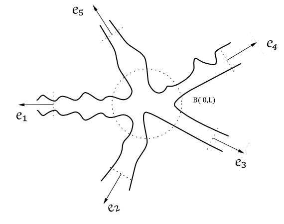
Figure 1: An example of a domain with 5 branches.

We go back to simple cases for recalling some known results with different geometrical conditions of $\Omega$. Let us replace the divergence-type operator $div(A\nabla u)$ by the Laplace operator together with Neumann boundary condition $\partial_{\nu}u:=\frac{\partial u}{\partial\nu}=0$ and set $q(x)\equiv 0$. Assume $f(x,u)=f(u)$ satisfying (1.8). That is,

$$\left\{\begin{array}[]{lll}&u_{t}-\Delta u=f(u),&t\in\mathbb{R},\ x\in\Omega,\\ &u_{\nu}=0,&t\in\mathbb{R},\ x\in\partial\Omega.\end{array}\right.$$ (1.13)

A simplest example of a domain with multiple branches is a straight infinite cylinder, that is, up to rotation,

$$\Omega=\big{\{}(x_{1},x^{\prime}):x_{1}\in\mathbb{R},\ x^{\prime}\in\omega\big{\}},$$ (1.14)

where $\omega\subset\mathbb{R}^{N-1}$ is a smooth bounded non-empty open connected subset of $\mathbb{R}^{N-1}$. From the pioneering paper [14], it is well known that (1.13) admits a planar front $\phi_{f}(x_{1}-c_{f}t)$ satisfying

$$c_{f}\phi_{f}^{\prime}+\phi_{f}^{\prime\prime}+f(\phi_{f})=0,\ \phi_{f}(-\infty)=1\hbox{ and }\phi_{f}(+\infty)=0.$$ (1.15)

The function $\phi_{f}$ is called the profile and the constant $c_{f}$ is called the propagation speed. It is also well-known that $\phi_{f}$ and $c_{f}$ are uniquely determined by $f$, $\phi_{f}$ is decreasing and $c_{f}$ is of the sign of $\int_{0}^{1}f(s)ds$.

Another particular example is a curved cylinder, that is, up to rotation,

$$\Omega=\big{\{}(x_{1},x^{\prime}):x_{1}\in\mathbb{R},\ x^{\prime}\in\omega(x_{1})\big{\}},$$ (1.16)

where $(\omega(x_{1}))_{x_{1}\in\mathbb{R}}$ is a family of smooth bounded non-empty open connected subset of $\mathbb{R}^{N-1}$. One can easily notice that the planar front $\phi_{f}(x_{1}-c_{f}t)$ is not a solution of (1.13) in general if $\omega(x_{1})$ is not independent of $x_{1}$. However, there still exist some front-like solutions. For instance, when $\Omega$ is a bilaterally straight cylinder, that is, $\omega(x_{1})$ is independent of $x_{1}$ for $x_{1}\leq-L$ and for $x_{1}\geq L$, with some $L>0$, there exist entire solutions emanating from the planar front $\phi_{f}(x_{1}-c_{f}t)$ coming from the “left” part of the domain, see [2, 8, 29]. More precisely, there exists a unique solution $u:\mathbb{R}\times\overline{\Omega}\to(0,1)$ of (1.13) such that

$$u(t,x)-\phi_{f}(x_{1}-c_{f}t)\rightarrow 0\,\text{ as }t\rightarrow-\infty\text{ uniformly in $\overline{\Omega}$}.$$ (1.17)

One can also refer to [29] for the existence of front-like solutions in asymptotically straight cylinders. If the curved cylinder $\Omega$ is with periodic boundaries, that is, $\omega(x_{1})$ is periodic with respect to $x_{1}\in\mathbb{R}$, there may also exist pulsating traveling fronts (as defined in the next paragraph), see [25] for some conditions of existence. For a general domain with multiple cylindrical branches (every branch is straight), one knows from [18] that there exist entire solutions emanating from planar fronts in some branches. In fact, let $I$ and $J$ be two non-empty sets of $\{1,\cdots,m\}$ ($m$ is the number of branches) such that $I\cap J=\emptyset$ and $I\cup J=\{1,\cdots,m\}$. There exists a time-increasing solution $u(t,x)$ of (1.13) such that

$$\left\{\begin{array}[]{rcll}u(t,x)\!-\!\phi_{f}(-x\cdot e_{i}\!-\!c_{f}t\!+\!\sigma_{i})&\!\!\!\to\!\!\!&0\!\!&\text{uniformly in $\overline{\mathcal{H}_{i}}\cap\overline{\Omega}\,$ for every $i\in I$},\vspace{3pt}\\ u(t,x)&\!\!\to\!\!&0\!\!&\displaystyle\text{uniformly in $\overline{\Omega\setminus\mathop{\bigcup}_{i\in I}\mathcal{H}_{i}}$},\end{array}\right.\text{as $t\rightarrow-\infty$}$$

for some real numbers $(\sigma_{i})_{i\in I}$.

We now recall some results regarding to the periodic heterogeneity of coefficients. Suppose that the coefficients $A(x)$, $q(x)$, the nonlinear function $f(x,u)$ and the domain $\Omega$ are periodic in the direction $e$. For convenience in presentation, assume that they are periodic in the sense that $A(x+ke)=A(x)$, $q(x+ke)=q(x)$, $f(x+ke,u)=f(x,u)$ and $\Omega+ke=\Omega$ for any $k\in\mathbb{Z}^{N}$. In this case, one can define pulsating fronts $u(t,x)$ for (1.3), see [3]. A pulsating front $u(t,x)$ facing direction $e$ is a classical solution of (1.3) such that for some $c\neq 0$, there holds

$$u(t-\frac{k}{c},x)=u(t,x+ke)\hbox{ for all $t\in\mathbb{R}$, $x\in\overline{\Omega}$},$$

and such that, for all $t\in\mathbb{R}$,

$$u(t,x)\rightarrow 1\hbox{ as }x\cdot e\rightarrow-\infty,\ u(t,x)\rightarrow 0\hbox{ as }x\cdot e\rightarrow+\infty.$$

Similarly, one can define a pulsating front facing direction $-e$. We refer to [10, 12, 16, 28, 35, 36, 37] for some existence results of pulsating fronts in the whole space $\Omega=\mathbb{R}^{N}$. We also refer to [9, 38, 40, 41] for nonexistence results. The heterogeneity of coefficients not only effects the profiles of pulsating fronts but also the propagation speeds. Generally speaking, the front facing direction $e$ is not the same as the front facing direction $-e$.

In this paper, we aim to deduce some existence and uniqueness results of solutions of (1.3) under rather general assumptions. For this purpose, we recall the notion of transition fronts which generalizes the standard notion of traveling fronts. Such notion covers the planar fronts, pulsating fronts and also many types of fronts in the whole space, such as conical shaped fronts, pyramidal fronts and so on, see [20, 21, 22, 23, 27, 32, 33, 34]. Let us first introduce a few notations. The unbounded open connected set $\Omega\subset\mathbb{R}^{N}$ is assumed to have a globally $C^{2,\beta}$ boundary with $\beta>0$ (this is what we call a smooth domain throughout the paper), that is, there exist $\rho>0$ and $C>0$ such that, for every $y\in\partial\Omega$, there are a rotation $R_{y}$ of $\mathbb{R}^{N}$ and a $C^{2,\beta}$ map $\psi_{y}:\bar{B}=\big{\{}x^{\prime}\in\mathbb{R}^{N-1}:|x^{\prime}|\leq 2\rho\big{\}}\rightarrow\mathbb{R}$ such that $\psi_{y}(0)=0$, $\|\psi_{y}\|_{C^{2,\beta}(\bar{B})}\leq C$ and

$$\Omega\cap B(y,\rho)=\left[y+R_{y}\big{(}\{x=(x^{\prime},x_{N})\in\mathbb{R}^{N}:x^{\prime}\in\bar{B},x_{N}>\psi_{y}(x^{\prime})\}\big{)}\right]\cap B(y,\rho),$$

where

$$B(y,\rho)=\big{\{}x\in\mathbb{R}^{N}:|x-y|<\rho\big{\}}$$

and $|\ \ |$ denotes the Euclidean norm. Let $d_{\Omega}$ be the geodesic distance in $\overline{\Omega}$. For any two subsets $A$ and $B$ of $\overline{\Omega}$, we set

$$d_{\Omega}(A,B)=\inf\big{\{}d_{\Omega}(x,y):(x,y)\in A\times B\big{\}},$$

and $d_{\Omega}(x,A)=d_{\Omega}(\{x\},A)$ for $x\in\mathbb{R}^{N}$. Consider now two families $(\Omega_{t}^{-})_{t\in\mathbb{R}}$ and $(\Omega_{t}^{+})_{t\in\mathbb{R}}$ of open non-empty subsets of $\Omega$ such that

$$\forall t\in\mathbb{R},\ \ \left\{\begin{array}[]{l}\Omega_{t}^{-}\cap\Omega_{t}^{+}=\emptyset,\vspace{3pt}\\ \partial\Omega_{t}^{-}\cap\Omega=\partial\Omega_{t}^{+}\cap\Omega=:\Gamma_{t},\vspace{3pt}\\ \Omega_{t}^{-}\cup\Gamma_{t}\cup\Omega_{t}^{+}=\Omega,\vspace{3pt}\\ \sup\big{\{}d_{\Omega}(x,\Gamma_{t}):x\in\Omega_{t}^{+}\big{\}}=\sup\big{\{}d_{\Omega}(x,\Gamma_{t}):x\in\Omega_{t}^{-}\big{\}}=+\infty\end{array}\right.$$ (1.22)

and

$$\left\{\begin{array}[]{l}\inf\Big{\{}\sup\big{\{}d_{\Omega}(y,\Gamma_{t}):y\in\Omega_{t}^{+},d_{\Omega}(y,x)\leq r\big{\}}:t\in\mathbb{R},\ x\in\Gamma_{t}\Big{\}}\rightarrow+\infty\vspace{3pt}\\ \inf\Big{\{}\sup\big{\{}d_{\Omega}(y,\Gamma_{t}):y\in\Omega_{t}^{-},d_{\Omega}(y,x)\leq r\big{\}}:t\in\mathbb{R},\ x\in\Gamma_{t}\Big{\}}\rightarrow+\infty\end{array}\right.\text{ as}\ \ r\rightarrow+\infty.$$ (1.25)

Notice that the condition (1.22) implies in particular that the interface $\Gamma_{t}$ is not empty for every $t\in\mathbb{R}$. As far as (1.25) is concerned, it says that for any $M>0$, there is $r_{M}>0$ such that, for every $t\in\mathbb{R}$ and $x\in\Gamma_{t}$, there are $y^{\pm}\in\mathbb{R}^{N}$ such that

$$y^{\pm}\in\Omega^{\pm}_{t},\ \ d_{\Omega}(x,y^{\pm})\leq r_{M}\ \ \text{and}\ \ d_{\Omega}(y^{\pm},\Gamma_{t})\geq M.$$ (1.26)

Moreover, in order to avoid interfaces with infinitely many twists, the sets $\Gamma_{t}$ are assumed to be included in finitely many graphs: there is an integer $n\geq 1$ such that, for each $t\in\mathbb{R}$, there are $n$ open subsets $\omega_{i,t}\subset\mathbb{R}^{N-1}$(for $1\leq i\leq n$), $n$ continuous maps $\psi_{i,t}:\omega_{i,t}\rightarrow\mathbb{R}$ and $n$ rotations $R_{i,t}$ of $\mathbb{R}^{N}$, with

$$\Gamma_{t}\subset\bigcup_{1\leq i\leq n}R_{i,t}\left(\big{\{}x=(x^{\prime},x_{N})\in\mathbb{R}^{N}:x^{\prime}\in\omega_{i,t},\ x_{N}=\psi_{i,t}(x^{\prime})\big{\}}\right).$$ (1.27)

Definition 1.1

[4, 5] For problem (1.3), a transition front connecting $0$ and $1$ is a classical solution $u:\mathbb{R}\times\overline{\Omega}\rightarrow(0,1)$ for which there exist some sets $(\Omega_{t}^{\pm})_{t\in\mathbb{R}}$ and $(\Gamma_{t})_{t\in\mathbb{R}}$ satisfying (1.22)-(1.27), and, for every $\varepsilon>0$, there exists $M_{\varepsilon}>0$ such that

$$\left\{\begin{array}[]{l}\forall\,t\in\mathbb{R},\ \ \forall\,x\in\overline{\Omega_{t}^{+}},\ \ \left(d_{\Omega}(x,\Gamma_{t})\geq M_{\varepsilon}\right)\Rightarrow\left(u(t,x)\geq 1-\varepsilon\right)\!,\vspace{3pt}\\ \forall\,t\in\mathbb{R},\ \ \forall\,x\in\overline{\Omega_{t}^{-}},\ \ \left(d_{\Omega}(x,\Gamma_{t})\geq M_{\varepsilon}\right)\Rightarrow\left(u(t,x)\leq\varepsilon\right)\!.\end{array}\right.$$ (1.30)

Furthermore, $u$ is said to have a global mean speed $\gamma$ $(\geq 0)$ if

$$\frac{d_{\Omega}(\Gamma_{t},\Gamma_{s})}{|t-s|}\rightarrow\gamma\ \ \text{as}\ \ |t-s|\rightarrow+\infty.$$ (1.31)

As far as the domain with multiple branches is concerned, one can smoothly extend every branch $\mathcal{H}_{i}$ for $-e_{i}$ part. Denote the extension of $\mathcal{H}_{i}$ by $\widetilde{\mathcal{H}}_{i}$. For instance, one can extend the $-e_{i}$ part of $\mathcal{H}_{i}$ to be

$$\widetilde{\mathcal{H}}_{i}:=\{x\in\mathbb{R}^{N};x-(x\cdot e_{i})e_{i}\in\widetilde{\omega}_{i}(x\cdot e_{i})\}+x_{i}$$ (1.32)

such that $|\widetilde{\omega}_{i}(s)|$ is uniformly bounded for $s\in\mathbb{R}$ and $\widetilde{\omega}_{i}(s)=\omega_{i}(s)$ for $s>0$. Moreover, one can redefine $A(x)$, $q(x)$, $f(x,u)$ to be $\widetilde{A}(x)$, $\widetilde{q}(x)$, $\widetilde{f}(x,u)$ in $\widetilde{\mathcal{H}}_{i}$ such that

$$\left\{\begin{array}[]{lll}&&\widetilde{A}(x)\in C^{1,\alpha}\hbox{ satisfies \eqref{eq-A}},\ \widetilde{q}(x)\in C^{0,\alpha}\hbox{ is bounded},\\ &&\widetilde{f}(x,u)\hbox{ is $C^{0,\alpha}$ in $x$ and $C^{1,\alpha}$ in $u$ satisfying $\widetilde{f}(x,0)=\widetilde{f}(x,1)=0$ and \eqref{eq-F}},\\ &&\widetilde{A}(x)=A(x),\ \widetilde{q}(x)=q(x),\ \widetilde{f}(x,u)=f(x,u)\hbox{ for $x\in\mathcal{H}_{i}$},\end{array}\right.$$ (1.36)

Notice that there are various ways of extension. As mentioned in front, for the following equation

$$\left\{\begin{array}[]{lll}&u_{t}-$div$(\widetilde{A}(x)\nabla u)+\widetilde{q}(x)\cdot\nabla u=\widetilde{f}(x,u),&t\in\mathbb{R},\ x\in\widetilde{\mathcal{H}}_{i},\\ &\nu\widetilde{A}(x)\nabla u=0,&t\in\mathbb{R},\ x\in\partial\widetilde{\mathcal{H}}_{i},\end{array}\right.$$ (1.39)

there are many possibilities of existence of front-like solutions including planar fronts and pulsating fronts. These fronts can actually be classified into the almost-planar front of the transition front, defined as following.

Definition 1.2

[4, 5] For a fixed $i\in\{1,\cdots,m\}$, assume that $\widetilde{\mathcal{H}}_{i}$ is a smooth extension of $\mathcal{H}_{i}$ and $\widetilde{A}(x)$, $\widetilde{q}(x)$, $\widetilde{f}(x,u)$ are redefined in $\widetilde{\mathcal{H}}_{i}$ such that (1.36) holds. A transition front $u(t,x)$ connecting $0$ and $1$ of (1.39) in the sense of Definition 1.1 is called almost-planar if, for every $t\in\mathbb{R}$, the set $\Gamma_{t}$ can be chosen as

$$\Gamma_{t}=\{x\in\widetilde{\mathcal{H}}_{i};x\cdot e_{i}=\xi_{t}\},$$

for some real number $\xi_{t}$. If $\Omega_{t}^{+}$ and $\Omega_{t}^{-}$ are defined by $\{x\in\widetilde{\mathcal{H}}_{i};x\cdot e_{i}\lessgtr\xi_{t}\}$ respectively, we call that $u(t,x)$ is facing direction $e_{i}$. If $\Omega^{+}_{t}$ and $\Omega_{t}^{-}$ are defined by $\{x\in\widetilde{\mathcal{H}}_{i};x\cdot e_{i}\gtrless\xi_{t}\}$ respectively, we call that $u(t,x)$ is facing direction $-e_{i}$.

For the existence of entire solutions emanating from almost-planar fronts in some branches and their large time behavior, we make rather general assumptions, that is, assume the existence and uniqueness of almost-planar fronts in every extended branch.

Assumption 1.3

For every $i\in\{1,\cdots,m\}$, assume that $\widetilde{\mathcal{H}}_{i}$ is a smooth extension of $\mathcal{H}_{i}$ and $\widetilde{A}(x)$, $\widetilde{q}(x)$, $\widetilde{f}(x,u)$ are redefined in $\widetilde{\mathcal{H}}_{i}$ such that (1.36) holds. Assume that there is a unique (up to time shifts) almost-planar front $u^{i}_{r}(t,x)$ connecting $0$ and $1$ of (1.39) facing to direction $e_{i}$ with sets $\Omega_{t}^{\pm}$ and $\Gamma_{t}$ satisfying

$$\Omega_{t}^{+}=\{x\in\widetilde{\mathcal{H}}_{i};x\cdot e_{i}<c^{i}_{r}t\},\ \Omega_{t}^{-}=\{x\in\widetilde{\mathcal{H}}_{i};x\cdot e_{i}>c^{i}_{r}t\}\hbox{ and }\Gamma_{t}=\{x\in\widetilde{\mathcal{H}}_{i};x\cdot e_{i}=c^{i}_{r}t\},$$

where $c^{i}_{r}$ is the propagation speed.

Assumption 1.4

For every $i\in\{1,\cdots,m\}$, assume that $\widetilde{\mathcal{H}}_{i}$ is a smooth extension of $\mathcal{H}_{i}$ and $\widetilde{A}(x)$, $\widetilde{q}(x)$, $\widetilde{f}(x,u)$ are redefined in $\widetilde{\mathcal{H}}_{i}$ such that (1.36) holds. Assume that there is a unique (up to time shifts) almost-planar front $u^{i}_{l}(t,x)$ connecting $0$ and $1$ of (1.39) facing to direction $-e_{i}$ with sets $\Omega_{t}^{\pm}$ and $\Gamma_{t}$ satisfying

$$\Omega_{t}^{+}=\{x\in\widetilde{\mathcal{H}}_{i};x\cdot e_{i}>-c^{i}_{l}t\},\ \Omega_{t}^{-}=\{x\in\widetilde{\mathcal{H}}_{i};x\cdot e_{i}<-c^{i}_{l}t\}\hbox{ and }\Gamma_{t}=\{x\in\widetilde{\mathcal{H}}_{i};x\cdot e_{i}=-c^{i}_{l}t\},$$

where $c^{i}_{l}$ is the propagation speed.

Remark 1.5

The uniqueness in Assumptions 1.3 and 1.4 means that if there is a transition front $v(t,x)$ with the same sets $\Gamma_{t}$ and $\Omega^{\pm}_{t}$ defined in Assumption 1.3 or 1.4, then there is $\tau\in\mathbb{R}$ such that $v(t,x)=u^{i}_{r}(t+\tau,x)$ or $v(t,x)=u^{i}_{l}(t+\tau,x)$ respectively.

Moreover, we need a technical assumption, that is,

Assumption 1.6

For any fixed $i\in\{1,\cdots,m\}$, take a sequence $\{t_{n}\}_{n\in\mathbb{N}}\subset\mathbb{R}$ such that $t_{n}\rightarrow+\infty$ as $n\rightarrow+\infty$. Let $\mathcal{H}_{i}^{n}=\mathcal{H}_{i}-t_{n}e_{i}$, $A_{n}(x)=A(x+t_{n}e_{i})$, $q_{n}(x)=q_{n}(x+t_{n}e_{i})$ and $f_{n}(x,\cdot)=f(x+t_{n}e_{i},\cdot)$ for $x\in\mathcal{H}_{i}^{n}$. Assume that for any such sequence $\{t_{n}\}_{n\in\mathbb{N}}$, there is an infinite cylinder $\mathcal{H}_{i}^{\infty}$ parallel to $e_{i}$ such that $\mathcal{H}_{i}^{n}$ converge locally uniformly to $\mathcal{H}_{i}^{\infty}$ and there are $A_{\infty}(x)$, $q_{\infty}(x)$, $f_{\infty}(x,\cdot)$ satisfying (1.36) such that $A_{n}\rightarrow A_{\infty}$, $q_{n}(x)\rightarrow q_{\infty}(x)$, $f_{n}\rightarrow f_{\infty}$ locally uniformly in $\mathcal{H}_{i}^{\infty}$ as $n\rightarrow+\infty$. Assume that there exist a unique (up to time shifts) almost planar front $v_{r}(t,x)$ facing direction $e_{i}$ and a unique almost planar front $v_{l}(t,x)$ facing direction $-e_{i}$ for the limiting equation

$$\left\{\begin{array}[]{lll}&v_{t}-$div$(A_{\infty}(x)\nabla v)+q_{\infty}(x)\cdot\nabla v=f_{\infty}(x,v),&t\in\mathbb{R},\ x\in\mathcal{H}_{i}^{\infty},\\ &\nu A_{\infty}(x)\nabla v=0,&t\in\mathbb{R},\ x\in\partial\mathcal{H}_{i}^{\infty}.\end{array}\right.$$

This assumption actually holds for many cases such as (i) $\mathcal{H}_{i}^{\infty}$ is a straight cylinder and $A_{\infty}$, $q_{\infty}$, $f_{\infty}(\cdot,s)$ (for every $s\in\mathbb{R}$) are constant, (ii) $\mathcal{H}_{i}^{\infty}$ is a straight cylinder and $A_{\infty}$, $q_{\infty}$, $f_{\infty}$ are independent of $x\cdot e_{i}$, (iii) $\mathcal{H}_{i}^{\infty}$, $A_{\infty}$, $q_{\infty}$, $f_{\infty}$ are periodic in $x\cdot e_{i}$, see [5, Theorem 1.14]. One can see Section 5 for some examples which satisfy all Assumptions 1.3, 1.4 and 1.6.

Now, we claim the existence of entire solutions emanating from almost-planar fronts in some branches.

Theorem 1.7

Let Assumptions 1.4 and 1.6 hold. Let $I$ and $J$ be two non-empty sets of $\{1,\cdots,m\}$ such that $I\cap J=\emptyset$ and $I\cup J=\{1,\cdots,m\}$. If $c^{i}_{l}>0$ for all $i\in I$, then there exists a time-increasing entire solution $u(t,x)$ of (1.3) such that

$$\left\{\begin{array}[]{rcll}u(t,x)\!-\!u^{i}_{l}(t+\sigma_{i},x)&\!\!\!\to\!\!\!&0\!\!&\text{uniformly in $\overline{\mathcal{H}_{i}}\cap\overline{\Omega}\,$ for every $i\in I$},\vspace{3pt}\\ u(t,x)&\!\!\to\!\!&0\!\!&\displaystyle\text{uniformly in $\overline{\Omega\setminus\mathop{\bigcup}_{i\in I}\mathcal{H}_{i}}$},\end{array}\right.$$ (1.41)

as $t\rightarrow-\infty$ for some real numbers $(\sigma_{i})_{i\in I}$.

We then investigate the large time behavior of the entire solution $u(t,x)$ in Theorem 1.7. By the standard parabolic estimates, one knows that there is a $C^{2}(\overline{\Omega})$ solution $p:\overline{\Omega}\rightarrow(0,1]$ of

$$\left\{\begin{array}[]{lll}&-$div$(A(x)\nabla p)+q(x)\cdot\nabla p=f(x,p),&x\in\Omega,\\ &\nu A(x)\nabla p=0,&t\in\mathbb{R},\ x\in\partial\Omega,\end{array}\right.$$ (1.44)

such that $u(t,x)\rightarrow p(x)$ as $t\rightarrow+\infty$ locally uniformly in $x\in\overline{\Omega}$. For the propagation in a domain with multiple cylindrical branches $\Omega$, two cases may occur, that is, the propagation is complete or blocked. Here, we mean the complete propagation by $p\equiv 1$ and we mean the blocked propagation by $p<1$. Both completely propagating and blocking phenomena have been proved to exist in many kinds of domains, such as exterior domains [6], bilaterally straight cylinders [2, 8, 30] and some periodic domains [11], under some geometrical conditions on domains respectively. Except the geometry of domains may block the propagation, the heterogeneity of the coefficients can also block the propagation, see [13]. If one treats the almost-planar front connecting $0$ and $1$ with positive propagation speed as an invasion of $0$ by $1$ in the sense of [5], then the negative propagation speed means $0$ invading $1$. The entire solution in Theorem 1.7 means that $1$ invades $0$ from branches $\mathcal{H}_{i}$. Similar as Theorem 1.7 and by providing Assumption 1.3, one can replace the roles of $0$ and $1$ through replacing $u$ and $f(x,u)$ by $1-u$ and $-f(x,1-u)$ to prove that if $c^{j}_{r}<0$ for some $j\in J$, $0$ invades $1$ from branches $\mathcal{H}_{j}$. In other words, $c^{j}_{r}<0$ implies that $1$ can not invade $0$ in branches $\mathcal{H}_{j}$, that is, the propagation is blocked.

Corollary 1.8

Let Assumptions 1.3, 1.4 and 1.6 hold. Let $I$ and $J$ be the non-empty sets and $u(t,x)$ be the entire solution satisfying (1.41) in Theorem 1.7. If $c^{i}_{r}<0$ for some $j\in J$, the solution $u(t,x)$ is blocked in $\mathcal{H}_{j}$, that is, $\sup_{x\in\mathcal{H}_{j}}p(x)<1$.

We assert in the following theorem that if the propagation of $u(t,x)$ is unblocked in some branches $\mathcal{H}_{j}$ for some $j\in J$, that is,

$$\liminf_{x\in\mathcal{H}_{j};\ x\cdot e_{j}\rightarrow+\infty}p(x)=1,$$ (1.45)

then $u(t,x)$ will eventually converge to the almost-planar front facing direction $e_{j}$ in $\mathcal{H}_{j}$.

Theorem 1.9

Let Assumptions 1.3, 1.4 and 1.6 hold. Let $I$ and $J$ be the non-empty sets and $u(t,x)$ be the entire solution satisfying (1.41) in Theorem 1.7. Assume that $J_{1}$ is a non-empty subset of $J$. If no blocking occurs in the branch $\mathcal{H}_{j}$ for all $j\in J_{1}$ in the sense of (1.45), then $c^{j}_{r}>0$ and the solution $u(t,x)$ converges to the almost-planar front facing direction $e_{j}$ in $\mathcal{H}_{j}$ for every $j\in J_{1}$ eventually, that is, there exist some real umbers $\tau_{j}$ such that

$$u(t,x)-u^{j}_{r}(t+\tau_{j},x)\rightarrow 0,$$

for $x\in\overline{\mathcal{H}_{j}}$ such that $x\cdot e_{j}\geq\varepsilon t$ as $t\rightarrow+\infty$, where $\varepsilon$ is an arbitrary positive constant.

Corollary 1.10

Let $u(t,x)$ be the entire solution in Theorem 1.9. If $u$ propagates completely in $\overline{\Omega}$, that is, $p\equiv 1$, then $J_{1}\equiv J$ and the entire solution $u(t,x)$ is a transition front connecting $0$ and $1$ with $(\Gamma_{t})_{t\in\mathbb{R}}$, $(\Omega^{\pm}_{t})_{t\in\mathbb{R}}$ defined by

$$\Gamma_{t}\!=\!\mathop{\bigcup}_{i\in I}\!\big{\{}x\!\in\!\mathcal{H}_{i}\cap\Omega:x\cdot e_{i}\!=\!c^{i}_{l}|t|\!+\!A\big{\}}\ (t\!\leq\!0),\ \Gamma_{t}\!=\!\mathop{\bigcup}_{j\in J_{1}}\!\big{\{}x\!\in\!\mathcal{H}_{j}\cap\Omega:x\cdot e_{j}\!=\!c^{j}_{r}t\!+\!A\big{\}}\ (t\!>\!0),$$ (1.46)

and

$$\left\{\begin{array}[]{llll}\displaystyle\Omega_{t}^{+}=\mathop{\bigcup}_{i\in I}\big{\{}x\in\mathcal{H}_{i}\cap\Omega:x\cdot e_{i}>c^{i}_{l}|t|+A\big{\}},&\Omega_{t}^{-}=\Omega\setminus\overline{\Omega_{t}^{+}},&\text{ for $t\leq 0$,}\vspace{3pt}\\ \displaystyle\Omega_{t}^{-}=\mathop{\bigcup}_{j\in J}\big{\{}x\in\mathcal{H}_{j}\cap\Omega:x\cdot e_{j}>c^{j}_{r}t+A\big{\}},&\Omega_{t}^{+}=\Omega\setminus\overline{\Omega_{t}^{-}},&\text{ for $t>0$,}\end{array}\right.$$ (1.49)

for some $A>0$. Moreover, there exist some real numbers $(\tau_{j})_{j\in J}$ such that

$$\left\{\begin{array}[]{rcll}u(t,x)-u^{j}_{r}(t+\tau_{j},x)&\!\!\!\to\!\!\!&0\!\!&\text{uniformly in $\overline{\mathcal{H}_{j}}\cap\overline{\Omega}\,$ for every $j\in J$},\vspace{3pt}\\ u(t,x)&\!\!\!\to\!\!\!&1\!\!&\displaystyle\text{uniformly in $\overline{\Omega\setminus\mathop{\bigcup}_{j\in J}\mathcal{H}_{j}}$},\end{array}\right.$$ (1.50)

as $t\rightarrow+\infty$.

Remark 1.11

Indeed, the conclusion of Corollary 1.10 covers the results of Theorem 1.7 in [18], where the almost-planar front in every branch is the planar front with the unique speed $c_{f}$.

Finally, we prove a general version of Conjecture 1.13 of [18], that is there is only one type of transition fronts connecting $0$ and $1$ by provided the complete propagation of any entire solution emanating from an almost-planar front in every branch. For each $i\in\{1,\cdots,m\}$, we denote by $u_{i}:\mathbb{R}\times\overline{\Omega}\rightarrow(0,1)$ the time-increasing solution of (1.3) emanating from the almost-planar front $u^{i}_{l}(t,x)$ in the branch $\mathcal{H}_{i}$, that is,

$$u_{i}(t,x)\rightarrow u^{i}_{l}(t,x)\mathop{\longrightarrow}_{t\to-\infty}0\hbox{ uniformly in $\overline{\mathcal{H}_{i}}\cap\overline{\Omega}$},\ u_{i}(t,x)\mathop{\longrightarrow}_{t\to-\infty}0\hbox{ uniformly in $\overline{\Omega\setminus\mathcal{H}_{i}}$}.$$ (1.51)

Theorem 1.12

Let Assumptions 1.3, 1.4 and 1.6 hold. If for every $i\in\{1,\cdots,m\}$, the entire solution $u_{i}$ of (1.51) propagates completely in the sense that $u_{i}(t,x)\rightarrow 1$ as $t\rightarrow+\infty$ locally uniformly in $\overline{\Omega}$, then any transition front of (1.3) connecting $0$ and $1$ is of the type (1.41), (1.46)-(1.49), that is, it emanates from the almost-planar fronts coming from some proper subset of branches as $t\to-\infty$ and it converges to the almost-planar fronts in the other branches as $t\to+\infty$.

Notice that Theorem 1.12 does not hold in general, without the assumption that every entire solution $u_{i}$ of (1.51) propagates completely, see the counter-example in Remark 1.10 of [18].

We organize this paper as following. In Section 2, we prove the existence of entire solutions emanating from almost-planar fronts in some branches, that is, Theorem 1.7. We also show Corollary 1.8 in this section. Section 3 is devoted to proving Theorem 1.9 and Corollary 1.10 which indicate the large time behavior of the entire solution of Theorem 1.7. In Section 4, we prove the uniqueness of the transition front connecting $0$ and $1$, that is, Theorem 1.12. Finally, we give some examples in Section 5, to which our results can be applied.

2 Existence of entire solutions

In this section, we only prove the existence of an entire solution emanating from one almost-planar front in one branch. The existence of entire solutions emanating from some almost-planar fronts in some branches, that is, Theorem 1.7, can be proved in a similar way. Indeed, from the following constructions of sub- and supersolutions, one knows that the constructions do not depend on the geometrical structure of the domain beyond the initiated branch. It means that one can construct sub- and supersolutions for some branches by simply combining the sub- and supersolutions in each branch of these branches. We assume without loss of generality that the branch $\mathcal{H}_{i}$ ($i$ could be any integer of $1,\cdots,m$) is the initiated branch, in which the entire solution emanating. By Assumption 1.4, one knows that for the extension $\widetilde{\mathcal{H}}_{i}$ of the branch $\mathcal{H}_{i}$, there is an almost-planar front $u^{i}_{l}(t,x)$ connecting $0$ and $1$ facing direction $-e_{i}$ of the equation (1.39). Assume that $c^{i}_{l}>0$. In the sequel, we are going to prove that there is an entire solution $u(t,x)$ such that

$$\left\{\begin{array}[]{rcll}u(t,x)\!-\!u^{i}_{l}(t,x)&\!\!\!\to\!\!\!&0\!\!&\text{uniformly in $\overline{\mathcal{H}_{i}}\cap\overline{\Omega}\,$},\vspace{3pt}\\ u(t,x)&\!\!\to\!\!&0\!\!&\displaystyle\text{uniformly in $\overline{\Omega\setminus\mathcal{H}_{i}}$},\end{array}\right.$$ (2.1)

as $t\rightarrow-\infty$.

2.1 Construction of sub- and supersolutions

We first need an auxiliary lemma which will be used frequently.

Lemma 2.1

For any $i\in\{1,\cdots,m\}$, assume that $\widetilde{\mathcal{H}}_{i}$ is a smooth extension of $\mathcal{H}_{i}$ and $\widetilde{A}(x)$, $\widetilde{q}(x)$, $\widetilde{f}(x,u)$ are redefined in $\widetilde{\mathcal{H}}_{i}$ such that (1.36) holds. Then, for any $\beta>0$, there exist $\lambda_{i}>0$ and a positive $C^{2}$ function $\psi_{i}(x)$ satisfying

$$\left\{\begin{array}[]{lll}&-$div$(\widetilde{A}(x)\nabla\psi_{i})+\lambda_{i}($div$(\widetilde{A}(x)e_{i}\psi_{i})+e_{i}\widetilde{A}\nabla\psi_{i})+\widetilde{q}(x)\cdot\nabla\psi_{i}&\\ &-\lambda_{i}\widetilde{q}(x)e_{i}\psi_{i}-\lambda_{i}^{2}(e_{i}\widetilde{A}(x)e_{i})\psi_{i}\geq-\beta\psi_{i},&x\in\widetilde{\mathcal{H}}_{i},\\ &\nu\widetilde{A}(x)(\lambda_{i}\psi_{i}(x)e_{i}+\nabla\psi_{i})\geq 0,&x\in\partial\widetilde{\mathcal{H}}_{i},\end{array}\right.$$ (2.5)

such that $0<\inf_{\widetilde{\mathcal{H}}_{i}}\psi_{i}(x)\leq\sup_{\widetilde{\mathcal{H}}_{i}}\psi_{i}(x)<+\infty$.

Proof. Take a positive bounded $C^{2}$ function $\widetilde{\psi}_{i}(x)$ such that $\partial_{\nu}\widetilde{\psi}_{i}\geq 1$ for $x\in\partial\widetilde{\mathcal{H}}_{i}$ and all of its derivatives $\nabla\widetilde{\psi}_{i}$, $\nabla^{2}\widetilde{\psi}_{i}$ are bounded in the sense of $L^{\infty}$ norm. One can apply the classical distance function in [17] to get a such function. Let $\psi_{i}(x)=\widetilde{\psi}_{i}(x)+C$ where $C$ is a positive constant. Notice that $\nabla\psi_{i}=\nabla\widetilde{\psi}_{i}$ and $\nabla^{2}\psi_{i}=\nabla^{2}\widetilde{\psi}_{i}$. For any $\beta>0$, one can take $C$ sufficiently large and $0<\lambda_{i}\leq 1/(\|\widetilde{\psi}_{i}\|_{L^{\infty}}+C)$ sufficiently small such that

$$\frac{1}{\psi_{i}(x)}\Big{(}-div(\widetilde{A}(x)\nabla\psi_{i})+\lambda_{i}(div(\widetilde{A}(x)e_{i}\psi_{i})+e_{i}\widetilde{A}\nabla\psi_{i})+\widetilde{q}(x)\cdot\nabla\psi_{i}\Big{)}-\lambda_{i}\|\widetilde{q}(x)\|-\lambda_{i}^{2}\beta_{2}+\beta\geq 0,$$ (2.6)

for all $x\in\widetilde{\mathcal{H}}_{i}$ where $\|q(x)\|=\sum_{1\leq i\leq N}\|q_{i}(x)\|_{L^{\infty}}$ and $\beta_{2}$ is defined in (1.4). Then, the first inequality of (2.5) holds by (2.6) and the second inequality of (2.5) holds by

$$\lambda_{i}\leq 1/(\|\widetilde{\psi}_{i}\|_{L^{\infty}}+C)\leq(\nu\cdot\nabla\psi_{i})/\psi_{i}=(\nu\cdot\nabla\widetilde{\psi}_{i})/\psi_{i}.$$

From above, it is obvious that $0<\inf_{\widetilde{\mathcal{H}}_{i}}\psi_{i}(x)\leq\sup_{\widetilde{\mathcal{H}}_{i}}\psi_{i}(x)<+\infty$. $\Box$

Moreover, we need the time-monotonicity property of $u^{i}_{l}(t,x)$.

Lemma 2.2

Let Assumptions 1.4 and 1.6 hold. If $c^{i}_{l}>0$, then $(u^{i}_{l})_{t}(t,x)>0$ for all $t\in\mathbb{R}$ and $x\in\widetilde{H}_{i}$ and for any positive constant $D$, there exist $T_{1}<0$ and $k>0$ such that $(u^{i}_{l})_{t}(t,x)\geq k$ for $t\leq T_{1}$ and $x\in\overline{\widetilde{H}_{i}}$ such that $|x\cdot e_{i}+c^{i}_{l}t|\leq D$.

Proof. Since $c^{i}_{l}>0$, one can easily verify that $u^{i}_{l}(t,x)$ is an invasion of $0$ by $1$ in the sense of Definition 1.4 of [4]. Then, by Theorem 1.11 of [4], one has that $u^{i}_{l}(t,x)$ is increasing in time $t$, that is, $(u^{i}_{l})_{t}(t,x)>0$.

Denote, up to rotation,

$$\widetilde{\mathcal{H}}_{i}:=\{(x_{1},x^{\prime})\in\mathbb{R}^{N};x^{\prime}\in\widetilde{\omega}_{i}(x_{1})\},$$

where $\widetilde{\mathcal{H}}_{i}=\mathcal{H}_{i}$ for $x_{1}>0$. Notice that

$$d_{\Omega}(x,y)\geq|x-y|\hbox{ and }\frac{d_{\Omega}(x,y)}{|x-y|}<+\infty\hbox{ for any $x$, $y\in\widetilde{\mathcal{H}}_{i}$}$$ (2.7)

since $|\widetilde{\omega}_{i}(s)|$ is uniformly bounded for $s\in\mathbb{R}$. By [4, Theorem 1.2], we have that for any positive constant $D$, there is $\eta\in(0,1/2]$ such that $\eta\leq u^{i}_{l}(t,x)\leq 1-\eta$ for any $t\in\mathbb{R}$ and $x\in\overline{\widetilde{H}_{i}}$ such that $|x_{1}+c^{i}_{l}t|\leq D$. Take any negative constant $T_{1}$. Now assume by contradiction that there exist sequences $\{t_{n}\}_{n\in\mathbb{N}}$ of $(-\infty,T_{1}]$ and $\{x_{n}\}_{n\in\mathbb{N}}=\{(x_{n1},x_{n}^{\prime})\}_{n\in\mathbb{N}}$ satisfying $|x_{n1}+c^{i}_{l}t_{n}|\leq D$ such that $(u^{i}_{l})_{t}(t_{n},x_{n})\rightarrow 0$. Then, either $t_{n}\rightarrow t_{*}\in(-\infty,T_{1}]$ or $t_{n}\rightarrow-\infty$ as $n\rightarrow+\infty$. For the former case, there is $x_{*}\in\overline{\widetilde{\mathcal{H}}_{i}}$ such that $x_{n}\rightarrow x_{*}$ as $n\rightarrow+\infty$. So, $(u^{i}_{l})_{t}(t_{*},x_{*})=0$. If $x_{*}\in\widetilde{\mathcal{H}}_{i}$, it contradicts $(u^{i}_{l})_{t}>0$ for all $t\in\mathbb{R}$ and $x\in\overline{\widetilde{\mathcal{H}}_{i}}$. Then, $x_{*}\in\partial\widetilde{\mathcal{H}}_{i}$ and the Hopf lemma implies that $\partial_{\nu}(u^{i}_{l})_{t}(t_{*},x_{*})<0$ which contradicts the boundary condition.

Then, if $t_{n}\rightarrow-\infty$ as $n\rightarrow+\infty$, $x_{n1}$ converges to $+\infty$ as $n\rightarrow+\infty$. Since $|\omega_{i}(s)|$ is bounded uniformly for $s\in\mathbb{R}$, there is $x^{\prime}_{*}\in\mathbb{R}^{N-1}$ such that $x^{\prime}_{n}\rightarrow x^{\prime}_{*}$ as $n\rightarrow+\infty$. Let $\mathcal{H}_{i}^{n}=\widetilde{\mathcal{H}}_{i}-x_{n1}e_{i}$, $A_{n}(x)=\widetilde{A}(x_{1}+x_{n1},x^{\prime})$, $q_{n}(x)=\widetilde{q}(x_{1}+x_{n1},x^{\prime})$ and $f_{n}(x,\cdot)=\widetilde{f}(x_{1}+x_{n1},x^{\prime},\cdot)$. Then, by Assumption 1.6, there is an infinite cylinder $\mathcal{H}_{i}^{\infty}$ parallel to $e_{i}$ such that $\mathcal{H}_{i}^{n}$ converge locally uniformly to $\mathcal{H}_{i}^{\infty}$ and there are $A_{\infty}(x)$, $q_{\infty}(x)$, $f_{\infty}(x,\cdot)$ satisfying (1.36) such that $A_{n}\rightarrow A_{\infty}$, $q_{n}\rightarrow q_{\infty}$, $f_{n}\rightarrow f_{\infty}$ locally uniformly in $\mathcal{H}_{i}^{\infty}$. Let $u_{n}(t,x)=u^{i}_{l}(t+t_{n},x_{1}+x_{n1},x^{\prime})$. Then, $(0,x^{\prime}_{n})\in\mathcal{H}_{i}^{n}$ and $(u_{n})_{t}(0,0,x_{n}^{\prime})\rightarrow 0$ as $n\rightarrow+\infty$. Since $u^{i}_{l}(t,x)$ is an almost-planar by Assumption 1.4, it follows from Definition 1.1 and (2.7) that for any $\varepsilon>0$, there is $M_{\varepsilon}>0$ such that

$$\left\{\begin{array}[]{lll}u^{i}_{l}(t,x)\geq 1-\varepsilon,&&\hbox{ for $t\in\mathbb{R}$ and $x\in\widetilde{\mathcal{H}}_{i}$ such that $x_{1}+c^{i}_{l}t\geq M_{\varepsilon}$},\\ u^{i}_{l}(t,x)\leq\varepsilon,&&\hbox{ for $t\in\mathbb{R}$ and $x\in\widetilde{\mathcal{H}}_{i}$ such that $x_{1}+c^{i}_{l}t\leq-M_{\varepsilon}$}.\end{array}\right.$$

Then, by $|x_{n1}+c^{i}_{l}t_{n}|\leq D$, one can easily check that

$$\left\{\begin{array}[]{lll}u_{n}(t,x)\geq 1-\varepsilon,&&\hbox{ for $t\in\mathbb{R}$ and $x\in\mathcal{H}^{n}_{i}$ such that $x_{1}+c^{i}_{l}t\geq M_{\varepsilon}+D$},\\ u_{n}(t,x)\leq\varepsilon,&&\hbox{ for $t\in\mathbb{R}$ and $x\in\mathcal{H}^{n}_{i}$ such that $x_{1}+c^{i}_{l}t\leq-M_{\varepsilon}-D$}.\end{array}\right.$$ (2.11)

It means that $u_{n}(t,x)$ is an almost-planar front facing $-e_{i}$ with speed $c^{i}_{l}$ for all $n$. By parabolic estimates, $u_{n}(t,x)$ converge, up to extraction of a subsequence, to a solution $u_{*}(t,x)$ of

$$\left\{\begin{array}[]{lll}&u_{t}-$div$(A_{\infty}(x)\nabla u)+q_{\infty}(x)\cdot\nabla u=f_{\infty}(x,u),&t\in\mathbb{R},\ x\in\mathcal{H}_{i}^{\infty},\\ &\nu A_{\infty}(x)\nabla u=0,&t\in\mathbb{R},\ x\in\partial\mathcal{H}_{i}^{\infty}.\end{array}\right.$$

Then, $u_{*}(t,x)=v_{l}(t,x)$ up to shifts by Assumption 1.6 and $v_{l}(t,x)$ is an almost-planar front facing $-e_{i}$ with speed $c^{i}_{l}$ by (2.11). Since $c^{i}_{l}>0$, one has that $(v_{l})_{t}>0$. However, $(0,x^{\prime}_{n})\rightarrow(0,x^{\prime}_{*})\in\mathcal{H}_{i}^{\infty}$ as $n\rightarrow+\infty$ and $v_{t}(0,0,x^{\prime}_{*})=(u_{*})_{t}(0,0,x^{\prime}_{*})=0$ which is a contradiction. This completes the proof. $\Box$

Similarly, one can get the following lemma for $u^{i}_{r}(t,x)$.

Lemma 2.3

Let Assumptions 1.3 and 1.6 hold. If $c^{i}_{r}>0$, then $(u^{i}_{r})_{t}(t,x)>0$ for all $t\in\mathbb{R}$ and $x\in\widetilde{H}_{i}$ and for any positive constant $D$, there exist $T_{2}>0$ and $k>0$ such that $(u^{i}_{r})_{t}(t,x)\geq k$ for $t\geq T_{2}$ and $x\in\overline{\widetilde{H}_{i}}$ such that $|x\cdot e_{i}-c^{i}_{r}t|\leq D$.

We then announce some parameters. Remember that $\mathcal{H}_{i}$ is the initiated branch and $i$ is a fixed integer of $1,\cdots,m$. For convenience, define

$$\mathcal{H}_{i}(R):=\{x\in\mathcal{H}_{i};x\cdot e_{i}\geq R\},$$

for any $R>0$. By Lemma 2.1, there exist $\lambda_{i}>0$ and $\psi_{i}(x)>0$ such that (2.5) holds for the extension $\widetilde{\mathcal{H}}_{i}$ of $\mathcal{H}_{i}$ and $\beta=\gamma$ where $\gamma$ is defined by (1.7). Notice that $v(x):=e^{-\lambda_{i}(x\cdot e_{i}-L)}\psi_{i}(x)$ satisfies

$$\left\{\begin{array}[]{lll}&-$div$(A(x)\nabla v)+q(x)\cdot\nabla v\geq-\gamma v,&x\in\mathcal{H}_{i}(L),\\ &\nu A(x)\nabla v\geq 0,&x\in\partial\mathcal{H}_{i}(L),\end{array}\right.$$ (2.15)

where $L$ is defined by (1.10). Let $\delta>0$ be a constant such that

$$\delta\leq\min\Big{(}\frac{\sigma}{2},\lambda_{i}c^{i}_{l}\Big{)}\hbox{ where $\sigma$ is defined in \eqref{eq-F}}.$$

Let $\widetilde{\delta}=\delta/\|\psi_{i}\|_{L^{\infty}(\overline{\mathcal{H}_{i}(L)})}$. Since $u^{i}_{l}(t,x)$ is an almost-planar front by Assumption 1.4, there is $M_{\delta}>0$ such that

$$\left\{\begin{array}[]{lll}u^{i}_{l}(t,x)\geq 1-\delta,&&\hbox{ for $t\in\mathbb{R}$ and $x\in\widetilde{\mathcal{H}}_{i}$ such that $x\cdot e_{i}+c^{i}_{l}t\geq M_{\delta}$},\\ u^{i}_{l}(t,x)\leq\delta,&&\hbox{ for $t\in\mathbb{R}$ and $x\in\widetilde{\mathcal{H}}_{i}$ such that $x\cdot e_{i}+c^{i}_{l}t\leq-M_{\delta}$}.\end{array}\right.$$ (2.18)

By Lemma 2.2, there exist $T_{1}<0$ and $k>0$ such that

$$(u^{i}_{l})_{t}(t,x)\geq k\hbox{ for $t\leq T_{1}$ and $x\in\widetilde{\mathcal{H}}_{i}$ such that $-M_{\delta}\leq x\cdot e_{i}+c^{i}_{l}t\leq M_{\delta}$}.$$ (2.19)

Let $\omega$ be a large positive constant such that

$$\omega k\geq(\gamma+M)e^{\lambda_{i}(M_{\delta}+L+1)},$$ (2.20)

where $M=\sup_{x\in\mathbb{R}^{N},u\in[0,1]}|f_{u}(x,u)|$. We now construct a subsolution as the following

$$\underline{u}(t,x)=\left\{\begin{array}[]{lll}\max\{u^{i}_{l}(\underline{\zeta}(t),x)-\widetilde{\delta}e^{-\lambda_{i}(x\cdot e_{i}-L)}\psi_{i}(x),0\},&&\hbox{ in $\overline{\mathcal{H}_{i}(L)}$}\\ 0,&&\hbox{ in $\overline{\Omega}\setminus\overline{\mathcal{H}_{i}(L)}$},\end{array}\right.$$

where $\underline{\zeta}(t)=t-\omega e^{\delta t}$.

Lemma 2.4

There exists $T<0$ such that $\underline{u}(t,x)$ is a subsolution of (1.3) for all $t\leq T$ and $x\in\overline{\Omega}$.

Proof. Take $T\leq T_{1}<0$ such that

$$c^{i}_{l}T<-L-M_{\delta^{\prime}},$$ (2.22)

where $\delta^{\prime}:=\widetilde{\delta}\inf_{x\in\widetilde{\mathcal{H}}_{i}}\psi(x)>0$ (one knows from Lemma 2.1 that $\inf_{x\in\widetilde{\mathcal{H}}_{i}}\psi(x)>0$) and $M_{\delta^{\prime}}$ is defined by (2.18) with $\delta$ replaced by $\delta^{\prime}$. Notice that $\underline{\zeta}(t)\leq T_{1}$ for all $t\leq T$. Let us first check that $\underline{u}(t,x)$ is well-defined and continuous for all $t\leq T$ and $x\in\overline{\Omega}$. Notice that the interfaces $\Gamma_{\xi}$ of $u_{l}^{i}(\xi,x)$ is defined by $\Gamma_{\xi}=\{x\in\widetilde{\mathcal{H}_{i}};x\cdot e_{i}=-c^{i}_{l}\xi\}$. Since $c^{i}_{l}\underline{\zeta}(t)<-L-M_{\delta^{\prime}}$ for $t\leq T$ by (2.22) and $\widetilde{\mathcal{H}_{i}}=\mathcal{H}_{i}$ for $x\cdot e_{i}\geq L$, one has $x\cdot e_{i}+c^{i}_{l}\underline{\zeta}(t)<-M_{\delta^{\prime}}$ for $t\leq T$ and $x\in\overline{\mathcal{H}_{i}}$ such that $x\cdot e_{i}\leq L$. Thus, it follows from (2.18) that

$$u^{i}_{l}(\underline{\zeta}(t),x)\leq\delta^{\prime}\hbox{ for $t\leq T$ and $x\in\overline{\mathcal{H}_{i}}$ such that $x\cdot e_{i}\leq L$}.$$

Meantime, on $x\in\overline{\mathcal{H}_{i}}$ such that $x\cdot e_{i}=L$, one has $\widetilde{\delta}e^{-\lambda_{i}(x\cdot e_{i}-L)}\psi_{i}(x)\geq\delta^{\prime}$. Therefore, $\underline{u}(t,x)=0$ for $t\leq T$ and $x\in\overline{\mathcal{H}_{i}}$ such that $x\cdot e_{i}=L$. By the definition of $\underline{u}(t,x)$, it is well-defined and continuous in $\overline{\Omega}$. Since $u^{i}_{l}(t,x)$ satisfies $\nu A(x)\nabla u^{i}_{l}(t,x)=0$ on $x\in\partial\mathcal{H}_{i}(L)$ and by (2.15), one knows that $\underline{u}(t,x)$ satisfies $\nu A(x)\nabla\underline{u}(t,x)\leq 0$ for any $t\leq T$ and $x\in\partial\Omega$.

To prove that $\underline{u}(t,x)$ is a subsolution, one only has to check that

$$N(t,x):=\underline{u}_{t}-\hbox{ div}(A(x)\nabla\underline{u})+q(x)\cdot\nabla\underline{u}-f(x,\underline{u})\leq 0,$$

for $t\leq T$ and $x\in\overline{\Omega}$ such that $\underline{u}(t,x)>0$. From above arguments, $\underline{u}(t,x)>0$ implies that $x\in\overline{\mathcal{H}_{i}(L)}$ and $\underline{u}(t,x)=u^{i}_{l}(\underline{\zeta}(t),x)-\widetilde{\delta}e^{-\lambda_{i}(x\cdot e_{i}-L)}\psi_{i}(x)$. Since $u^{i}_{l}(t,x)$ satisfies (1.3) for $x\in\overline{\mathcal{H}_{i}(L)}$, it follows from some calculations and (2.15) that

$$N(t,x)\leq-\omega\delta e^{\delta t}(u^{i}_{l})_{t}(\underline{\zeta}(t),x)+\gamma\widetilde{\delta}e^{-\lambda_{i}(x\cdot e_{i}-L)}\psi_{i}(x)+f(x,u^{i}_{l}(\underline{\zeta}(t),x))-f(x,\underline{u}(t,x)).$$

For $t\leq T$ and $x\in\overline{\mathcal{H}_{i}(L)}$ such that $x\cdot e_{i}+c^{i}_{l}\underline{\zeta}(t)\leq-M_{\delta}$, it follows that $0<u^{i}_{l}(\underline{\zeta}(t),x)\leq\delta$ and $\underline{u}(t,x)\leq\delta$. Then, by $\delta\leq\sigma/2$ and (1.7),

$$f(x,u^{i}_{l}(\underline{\zeta}(t),x))-f(x,\underline{u}(t,x))\leq-\gamma\widetilde{\delta}e^{-\lambda_{i}(x\cdot e_{i}-L)}\psi_{i}(x).$$

Thus,

$$N(t,x)\leq-\omega\delta e^{\delta t}(u^{i}_{l})_{t}(\underline{\zeta}(t),x)+\Big{(}\gamma-\gamma\Big{)}\widetilde{\delta}e^{-\lambda_{i}(x\cdot e_{i}-L)}\psi_{i}(x)\leq 0,$$

by $(u^{i}_{l})_{t}>0$. For $t<T$ and $x\in\overline{\mathcal{H}_{i}(L)}$ such that $x\cdot e_{i}+c^{i}_{l}\underline{\zeta}(t)\geq M_{\delta}$, it follows that $u^{i}_{l}(\underline{\zeta}(t),x)\geq 1-\delta$ and $\underline{u}(t,x)\geq 1-2\delta$. Then, by $\delta\leq\sigma/2$ and (1.7),

$$f(x,u^{i}_{l}(\underline{\zeta}(t),x))-f(x,\underline{u}(t,x))\leq-\gamma\widetilde{\delta}e^{-\lambda_{i}(x\cdot e_{i}-L)}\psi_{i}(x).$$

Thus,

$$N(t,x)\leq-\omega\delta e^{\delta t}(u^{i}_{l})_{t}(\underline{\zeta}(t),x)+\Big{(}\gamma-\gamma\Big{)}\widetilde{\delta}e^{-\lambda_{i}(x\cdot e_{i}-L)}\psi_{i}(x)\leq 0,$$

by $(u^{i}_{l})_{t}>0$.

Finally, for $t\leq T$ and $x\in\overline{\mathcal{H}_{i}(L)}$ such that $-M_{\delta}\leq x\cdot e_{i}+c^{i}_{l}\underline{\zeta}(t)\leq M_{\delta}$, one has $(u^{i}_{l})_{t}(\underline{\zeta}(t),x)\geq k>0$ where $k$ is defined by (2.19). It also implies that $x\cdot e_{i}\geq-c^{i}_{l}(t-\omega e^{\delta t})-M_{\delta}$ and hence $e^{-\lambda_{i}(x\cdot e_{i}-L)}\leq e^{\lambda_{i}c^{i}_{l}t}e^{\lambda_{i}(M_{\delta}+L)}$. It is obvious that

$$f(x,u^{i}_{l}(\underline{\zeta}(t),x))-f(x,\underline{u}(t,x))\leq M\widetilde{\delta}e^{-\lambda_{i}(x\cdot e_{i}-L)}\psi_{i}(x),$$

where $M=\sup_{x\in\mathbb{R}^{N},u\in[0,1]}|f_{u}(x,u)|$. Therefore,

$$N(t,x)\leq -k\omega\delta e^{\delta t}+\gamma\widetilde{\delta}e^{-\lambda_{i}(x\cdot e_{i}-L)}\psi_{i}(x)+M\widetilde{\delta}e^{-\lambda_{i}(x\cdot e_{i}-L)}\psi_{i}(x)$$

$$\leq -k\omega\delta e^{\delta t}+(\gamma+M)\widetilde{\delta}e^{\lambda_{i}c^{i}_{l}t}e^{\lambda_{i}(M_{\delta}+L)}\psi_{i}(x)\leq 0,$$

by $\delta\leq\lambda_{i}c^{i}_{l}$, $\widetilde{\delta}\psi_{i}(x)\leq\delta$ and (2.20). This completes the proof. $\Box$

Take any small $\varepsilon>0$ (at least $\varepsilon<\delta^{\prime}=\widetilde{\delta}\inf_{x\in\widetilde{\mathcal{H}}_{i}}\psi(x)$). Let $L_{\varepsilon}\geq L$ large enough such that $\delta e^{-\lambda_{i}(L_{\varepsilon}-L)}\leq\varepsilon/2$. We now construct supersolutions as the following

$$\overline{u}_{1}(t,x)=u_{l}^{i}(\overline{\zeta}(t),x)+\widetilde{\delta}e^{-\lambda_{i}(x\cdot e_{i}-L)}\psi_{i}(x),\hbox{ in $\overline{\mathcal{H}_{i}(L)}$},$$

where $\overline{\zeta}(t)=t+\omega e^{\delta t}$ and $\omega$ is defined by (2.20), and

$$\overline{u}_{2}(t,x)=\varepsilon\hbox{ for $x\in\overline{\mathcal{H}_{i}}$ such that $x\cdot e_{i}\leq L_{\varepsilon}$ and $x\in\overline{\Omega}\setminus\overline{\mathcal{H}_{i}}$}.$$

Lemma 2.5

There exists $T_{\varepsilon}<0$ such that $\overline{u}_{1}(t,x)$ is a supersolution of (1.3) for $t\leq T_{\varepsilon}$ and $x\in\overline{\mathcal{H}_{i}(L)}$ and $\overline{u}_{2}(t,x)$ is a supersolution of (1.3) for $t\leq T_{\varepsilon}$ and $x\in\overline{\mathcal{H}_{i}}$ such that $x\cdot e_{i}\leq L_{\varepsilon}$ and $x\in\overline{\Omega}\setminus\overline{\mathcal{H}_{i}}$.

Proof. Take $T_{\varepsilon}\leq T_{1}-\omega<0$ such that $c^{i}_{l}\omega e^{\delta t}\leq 1$ for all $t\leq T_{\varepsilon}$ and

$$c_{l}^{i}T_{\varepsilon}\leq-L_{\varepsilon}-M_{\varepsilon/2}-1,$$

where $M_{\varepsilon/2}$ is defined by (2.18) with $\delta$ replaced by $\varepsilon/2$. Notice that $\overline{\zeta}(t)\leq T_{1}$ for all $t\leq T_{\varepsilon}$. Since $f(x,\varepsilon)<0$ by $\varepsilon<\delta^{\prime}<\delta<\sigma$, one can easily find that $\overline{u}_{2}(t,x)$ is a supersolution of (1.3) for $t\leq T_{\varepsilon}$ and $x\in\overline{\mathcal{H}_{i}}$ such that $x\cdot e_{i}\leq L_{\varepsilon}$ and $x\in\overline{\Omega}\setminus\overline{\mathcal{H}_{i}}$. Obviously, $\overline{u}_{1}(t,x)$ is of $C^{2}$ in $\overline{\mathcal{H}_{i}(L)}$. By $\nu A(x)\nabla u^{i}_{l}(t,x)=0$ on $\partial\mathcal{H}_{i}(L)$ and (2.15), it follows that $\nu A(x)\nabla\overline{u}_{1}(t,x)\geq 0$ for any $t\leq T_{\varepsilon}$ and $x\in\partial\mathcal{H}_{i}(L)$.

Now, we check that

$$N(t,x):=\overline{u}_{1t}-\hbox{div}(A(x)\nabla\overline{u}_{1})+q(x)\cdot\nabla\overline{u}_{1}-f(x,\overline{u}_{1})\geq 0,$$

for $t\leq T_{\varepsilon}$ and $x\in\overline{\mathcal{H}_{i}(L)}$. By some calculation, one can obtain that

$$N(t,x)\geq\omega\delta e^{\delta t}(u^{i}_{l})_{t}(\overline{\zeta}(t),x)-\gamma\widetilde{\delta}e^{-\lambda_{i}(x\cdot e_{i}-L)}\psi_{i}(x)+f(x,u^{i}_{l}(\overline{\zeta}(t),x))-f(x,\overline{u}_{1}(t,x)),$$

since $u^{i}_{l}(t,x)$ satisfies (1.3) for $x\in\overline{\mathcal{H}_{i}(L)}$ and by (2.15). For $t\leq T_{\varepsilon}$ and $x\in\overline{\mathcal{H}_{i}(L)}$ such that $x\cdot e_{i}+c^{i}_{l}\overline{\zeta}(t)\leq-M_{\delta}$, it follows that $0<u^{i}_{l}(\overline{\zeta}(t),x)\leq\delta$. Thus, $\overline{u}_{1}(t,x)\leq 2\delta\leq\sigma$ since $\widetilde{\delta}e^{-\lambda_{i}(x\cdot e_{i}-L)}\psi_{i}(x)\leq\widetilde{\delta}\psi_{i}(x)<\delta$. Then, by (1.7),

$$f(x,u^{i}_{l}(\overline{\zeta}(t),x)-f(x,\overline{u}_{1}(t,x))\geq\gamma\widetilde{\delta}e^{-\lambda_{i}(x\cdot e_{i}-L)}\psi_{i}(x).$$

Thus,

$$N(t,x)\geq\omega\delta e^{\delta t}(u^{i}_{l})_{t}(\overline{\zeta}(t),x)+\Big{(}-\gamma+\gamma\Big{)}\widetilde{\delta}e^{-\lambda_{i}(x\cdot e_{i}-L)}\psi_{i}(x)\geq 0,$$

by $(u^{i}_{l})_{t}>0$. For $t\leq T_{\varepsilon}$ and $x\in\overline{\mathcal{H}_{i}(L)}$ such that $x\cdot e_{i}+c^{i}_{l}\overline{\zeta}(t)\geq M_{\delta}$, it follows that $u^{i}_{l}(\overline{\zeta}(t),x)\geq 1-\delta$ and $\overline{u}_{1}(t,x)\geq 1-\delta\geq 1-\sigma$. Then, by (1.7),

$$f(x,u^{i}_{l}(\overline{\zeta}(t),x))-f(x,\underline{u}_{1}(t,x))\geq\gamma\widetilde{\delta}e^{-\lambda_{i}(x\cdot e_{i}-L)}\psi_{i}(x).$$

Thus,

$$N(t,x)\geq\omega\delta e^{\delta t}(u^{i}_{l})_{t}(\overline{\zeta}(t),x)+\Big{(}-\gamma+\gamma\Big{)}\widetilde{\delta}e^{-\lambda_{i}(x\cdot e_{i}-L)}\psi_{i}(x)\geq 0,$$

by $(u^{i}_{l})_{t}>0$.

Finally, for $t\leq T_{\varepsilon}$ and $x\in\overline{\mathcal{H}_{i}(L)}$ such that $-M_{\delta}\leq x\cdot e_{i}+c^{i}_{l}\overline{\zeta}(t)\leq M_{\delta}$, one has $(u^{i}_{l})_{t}(\overline{\zeta}(t),x)\geq k>0$ where $k$ is defined by (2.19). It also implies that $x\cdot e_{i}\geq-c^{i}_{l}\overline{\zeta}(t)-M_{\delta}\geq-c^{i}_{l}t-1-M_{\delta}$ since $c^{i}_{l}\omega e^{\delta t}\leq 1$ for $t\leq T_{\varepsilon}$ and hence $e^{-\lambda_{i}(x\cdot e_{i}-L)}\leq e^{\lambda_{i}c^{i}_{l}t}e^{\lambda_{i}(M_{\delta}+L+1)}$. It is obvious that

$$f(x,u^{i}_{l}(\overline{\zeta}(t),x))-f(x,\overline{u}_{1}(t,x))\geq-M\widetilde{\delta}e^{-\lambda_{i}(x\cdot e_{i}-L)}\psi_{i}(x),$$

where $M=\sup_{x\in\mathbb{R}^{N},u\in[0,1]}|f_{u}(x,u)|$. Therefore,

$$N(t,x)\geq k\omega\delta e^{\delta t}-\gamma\widetilde{\delta}e^{-\lambda_{i}(x\cdot e_{i}-L)}\psi_{i}(x)-M\widetilde{d}e^{-\lambda_{i}(x\cdot e_{i}-L)}\psi_{i}(x)$$

$$\geq k\omega\delta e^{\delta t}-(\gamma+M)\widetilde{\delta}e^{\lambda_{i}c^{i}_{l}t}e^{\lambda_{i}(M_{\delta}+L+1)}\psi_{i}(x)\geq 0,$$

by $\delta\leq\lambda_{i}c^{i}_{l}$, $\widetilde{\delta}\psi_{i}(x)\leq\delta$ and (2.20). This completes the proof. $\Box$

Notice that $\overline{u}_{1}(t,x)\geq\delta^{\prime}>\varepsilon$ for all $t\leq T_{\varepsilon}$ and $x\in\overline{\mathcal{H}_{i}}$ such that $x\cdot e_{i}=L$. By the definition of $L_{\varepsilon}$, we know that $\widetilde{\delta}e^{-\lambda_{i}(x\cdot e_{i}-L)}\psi_{i}(x)\leq\varepsilon/2$ for $x\in\overline{\mathcal{H}_{i}(L)}$ such that $x\cdot e_{i}=L_{\varepsilon}$. By the definition of $T_{\varepsilon}$, one has that $x\cdot e_{i}+c^{i}_{l}\overline{\zeta}(t)\leq-M_{\varepsilon/2}$ for $t\leq T_{\varepsilon}$ and $x\in\overline{\mathcal{H}_{i}(L)}$ such that $x\cdot e_{i}=L_{\varepsilon}$. Thus, $u_{l}^{i}(\overline{\zeta}(t),x)\leq\varepsilon/2$ and hence $\overline{u}_{1}(t,x)\leq\varepsilon$ for $t\leq T_{\varepsilon}$ and $x\in\overline{\mathcal{H}_{i}(L)}$ such that $x\cdot e_{i}=L_{\varepsilon}$. Let

$$\overline{u}(t,x)=\left\{\begin{array}[]{lll}\overline{u}_{1}(t,x),&&\hbox{ for $t\leq T_{\varepsilon}$ and $x\in\overline{\mathcal{H}_{i}(L_{\varepsilon})}$}\\ \min\{\overline{u}_{1}(t,x),\overline{u}_{2}(t,x)\},&&\hbox{ for $t\leq T_{\varepsilon}$ and $x\in\overline{\mathcal{H}_{i}(L)}$ such that $x\cdot e_{i}\leq L_{\varepsilon}$},\\ \overline{u}_{2}(t,x),&&\hbox{for $t\leq T_{\varepsilon}$ and $x\in\overline{\Omega}\setminus\overline{\mathcal{H}_{i}(L)}$}\end{array}\right.$$

which is well-defined by above analysis. Moreover, it is a supersolution of (1.3) for $t\leq T_{\varepsilon}$ and $x\in\overline{\Omega}$ by Lemma 2.5 and the maximum principle.

2.2 Existence, monotonicity and uniqueness of the entire solution

We now prove the existence of an entire solution satisfying (2.1). Consider a sequence of solutions $u_{n}$ of (1.3) for $t>-n$ with initial value

$$u_{n}(-n,x)=\underline{u}(-n,x).$$

It is obvious that $\underline{u}(t,x)$ is increasing in $t$ for $t$ negative enough and $\underline{u}(t,x)\leq\overline{u}(t,x)$. Even if it means decreasing $T_{\varepsilon}$, assume $T_{\varepsilon}\leq T$ where $T$ and $T_{\varepsilon}$ are defined by Lemma 2.4 and Lemma 2.5 respectively. Then, it follows from the comparison principle that

$$\underline{u}(t,x)\leq u_{n}(t,x)\leq\overline{u}(t,x)\hbox{ for $-n\leq t<T_{\varepsilon}$ and $x\in\Omega$},$$ (2.24)

and

$$u_{n}(t,x)\geq u_{n-1}(t,x)\hbox{ for all $t\in[-n+1,+\infty)$, $x\in\Omega$}.$$

Using the monotonicity of the sequence and parabolic estimates on $u_{n}$, we have that the sequence $u_{n}$ converges to an entire solution $u(t,x)$ of (1.3). By (2.24), the solution $u(t,x)$ satisfies

$$\underline{u}(t,x)\leq u(t,x)\leq\overline{u}(t,x)\hbox{ for all $t\in(-\infty,T_{\varepsilon})$ and $x\in\Omega$}.$$

By definition of $\underline{u}$, $\overline{u}$ and remembering that $\varepsilon$ can be arbitrary small, one then has that

$$\left\{\begin{array}[]{rcll}u(t,x)\!-\!u^{i}_{l}(t,x)&\!\!\!\to\!\!\!&0\!\!&\text{uniformly in $\overline{\mathcal{H}_{i}}\cap\overline{\Omega}\,$},\vspace{3pt}\\ u(t,x)&\!\!\to\!\!&0\!\!&\displaystyle\text{uniformly in $\overline{\Omega\setminus\mathcal{H}_{i}}$},\end{array}\right.$$

as $t\rightarrow-\infty$. Since $\underline{u}_{t}>0$ for $t$ negative enough, it follows from the maximum principle that $(u_{n})_{t}>0$ for $t>-n$ and $x\in\Omega$. Passing to the limit $n\rightarrow+\infty$, one gets that $u_{t}\geq 0$ for $t\in\mathbb{R}$ and $x\in\Omega$. Again by the maximum principle, either $u_{t}>0$ or $u_{t}\equiv 0$. Since $u(t,x)\rightarrow u_{l}^{i}(t,x)$ in $\overline{\mathcal{H}_{i}}\cap\overline{\Omega}$ as $t\rightarrow-\infty$ and $(u^{i}_{l})_{t}>0$, $u_{t}\equiv 0$ is impossible. Therefore, $u_{t}>0$ for $t\in\mathbb{R}$ and $x\in\Omega$.

For any $0<\delta\leq 1/2$, define

$$\Omega_{\delta}(t)=\{x\in\Omega;\delta\leq u(t,x)\leq 1-\delta\}.$$

One can apply the proof of Lemma 2.2 to get the following lemma.

Lemma 2.6

For all $\delta\in(0,1/2]$, there exist $T_{\delta}<0$ and $k>0$ such that

$$u_{t}(t,x)\geq k\hbox{ for all $t\in(-\infty,T_{\delta}]$ and $x\in\Omega_{\delta}(t)$.}$$

Remark 2.7

Since $u(t,x)$ satisfies (2.1), one can take $T_{\delta}$ negative enough such that $\Omega_{\delta}(t)\subset\{x\in\mathcal{H}_{i};|x\cdot e_{i}+x^{i}_{l}t|\leq D\}$ for $t\leq T_{\delta}$ and some $D>0$.

Now, we prove the uniqueness of the entire solution $u$. Let $\delta>0$ be defined as in Section 2.1. Assume that there is another entire solution $v(t,x)$ satisfying (2.1). Then, for any $0<\varepsilon<\delta$, there is $t_{\varepsilon}<0$ such that

$$\sup_{x\in\Omega}|u(t,x)-v(t,x)|\leq\varepsilon,\hbox{ for any $t\leq t_{\varepsilon}$}.$$

For any $t_{0}\leq\min(t_{\varepsilon},T_{\delta}-\omega\varepsilon)$, define

$$u^{+}(t,x)=u(t_{0}+t+\omega\varepsilon(1-e^{-\delta t}),x)+\varepsilon e^{-\delta t}\hbox{ and }u^{-}(t,x)=u(t_{0}+t-\omega\varepsilon(1-e^{-\delta t}),x)-\varepsilon e^{-\delta t},$$

where $\omega>0$ is a constant such that $\omega k\delta\geq\delta+M$, $k$ is defined by Lemma 2.6 and $M=\sup_{x\in\mathbb{R}^{N},u\in[0,1]}|f_{u}(x,u)|$. One can check that $u^{+}(t,x)$ and $u^{-}(t,x)$ are sup- and subsolutions of the problem satisfied by $v(t_{0}+t,x)$ for $t\in[0,T_{\delta}-t_{0}-\omega\varepsilon]$. We omit the details of the checking process by referring to similar arguments as in Section 3 of [6]. Then, by the comparison principle, one has that

$$u^{-}(t,x)\leq v(t_{0}+t,x)\leq u^{+}(t,x),\hbox{ for $t\in[0,T_{\delta}-t_{0}-\omega\varepsilon]$ and $x\in\Omega$}.$$

It implies that

$$u(t-\omega\varepsilon(1-e^{-\delta(t-t_{0})}),x)-\varepsilon e^{-\delta(t-t_{0})}\leq v(t,x)\leq u(t+\omega\varepsilon(1-e^{-\delta(t-t_{0})}),x)+\varepsilon e^{-\delta(t-t_{0})},$$

for $t\in[t_{0},T_{\delta}-\omega\varepsilon]$ and $x\in\Omega$. As $t_{0}\rightarrow-\infty$, one gets that

$$u(t-\omega\varepsilon,x)\leq v(t,x)\leq u(t+\omega\varepsilon,x)$$ (2.25)

for all $t\in(-\infty,T_{\delta}-\omega\varepsilon]$ and $x\in\Omega$. Again by the comparison principle, (2.25) holds for all $t\in\mathbb{R}$ and $x\in\Omega$. Since $\varepsilon$ is arbitrary, we then get that $v(t,x)\equiv u(t,x)$. This completes the proof of the uniqueness of the entire solution satisfying (2.1).

2.3 Proof of Corollary 1.8

We complete this section by proving Corollary 1.8.

Proof of Corollary 1.8. Let $u(t,x)$ be the entire solution satisfying (1.41). Assume that $c^{j}_{r}<0$ for some $j\in J=\{1,\cdots,m\}\setminus I$. By replacing $u$ and $f(x,u)$ by $1-u$ and $-f(x,1-u)$ and applying the same arguments as in Section 2.1 and Section 2.2, one can prove that there is an entire solution $v(t,x)$ of (1.3) satisfying

$$\left\{\begin{array}[]{rcll}v(t,x)\!-\!u^{j}_{r}(t,x)&\!\!\!\to\!\!\!&0\!\!&\text{uniformly in $\overline{\mathcal{H}_{j}}\cap\overline{\Omega}\,$},\vspace{3pt}\\ v(t,x)&\!\!\to\!\!&1\!\!&\displaystyle\text{uniformly in $\overline{\Omega\setminus\mathcal{H}_{j}}$},\end{array}\right.$$

as $t\rightarrow-\infty$ and $v(t,x)$ is decreasing as $t$ increases. Then, for any $\varepsilon>0$, there is $t_{\varepsilon}<0$ such that

$$v(t,x)\geq 1-\varepsilon\hbox{ for $t\leq t_{\varepsilon}$ and $x\in\overline{\Omega\setminus\mathcal{H}_{j}}$},$$

and

$$u(t,x)\leq\varepsilon\hbox{ for $t\leq t_{\varepsilon}$ and $x\in\overline{\Omega\setminus\mathop{\bigcup}_{i\in I}\mathcal{H}_{i}}$}.$$

Since $I\cap J=\emptyset$ and $u(t,x)\leq 1$ for all $t\in\mathbb{R}$ and $x\in\overline{\Omega}$, one has that

$$u(t_{0},x)-\varepsilon\leq v(t_{0},x),\hbox{ for all $x\in\overline{\Omega}$},$$

where $t_{0}\leq\min(t_{\varepsilon},T_{\delta}-\omega\varepsilon)$, $\delta$, $\omega$, $T_{\delta}$ are parameters as defined in Section 2.2. Then, by similar arguments as in Section 3 of [6], one can easily check that the function

$$u^{-}(t,x)=u(t_{0}+t-\omega\varepsilon(1-e^{-\delta t}),x)-\varepsilon e^{-\delta t}$$

is a subsolution of the problem satisfied by $v(t+t_{0},x)$ for $t\in[0,T_{\delta}-t_{0}-\omega\varepsilon]$. It follows from the comparison principle that

$$u(t-\omega\varepsilon(1-e^{-\delta(t-t_{0})}),x)-\varepsilon e^{-\delta(t-t_{0})}\leq v(t,x),$$

for $t\in[t_{0},T_{\delta}-\omega\varepsilon]$ and $x\in\Omega$. As $t_{0}\rightarrow-\infty$, one obtains that

$$u(t-\omega\varepsilon,x)\leq v(t,x),\hbox{ for $t\in(-\infty,T_{\delta}-\omega\varepsilon]$ and $x\in\Omega$.}$$

Again by the comparison principle, the above inequality holds for all $t\in\mathbb{R}$ and $x\in\Omega$. As $\varepsilon\rightarrow 0$, we gets that

$$u(t,x)\leq v(t,x)\hbox{ for all $t\in\mathbb{R}$ and $x\in\Omega$}.$$

By the properties of the almost-planar front $u^{j}_{r}(t,x)$ and since $v(t,x)$ is decreasing in time, it follows that

$$\sup_{x\in\mathcal{H}_{j}}u(t,x)\leq\sup_{x\in\mathcal{H}_{j}}v(t,x)<1\hbox{ for all $t\in\mathbb{R}$}.$$

This completes the proof. $\Box$

3 Large time behavior of entire solutions

In this section, let $u(t,x)$ be the entire solution emanating from some almost-planar fronts in branches $\mathcal{H}_{i}$ ($i\in I$), that is, satisfying (1.41). Let $J=\{1,\cdots,m\}\setminus I$ and $J_{1}$ be a non-empty subset of $J$. We assume that the propagation of $u(t,x)$ is not blocked by branches $\mathcal{H}_{j}$ for all $j\in J_{1}$, that is,

$$\hbox{$u(t,x)\rightarrow p(x)$ as $t\rightarrow+\infty$ and }\liminf_{x\in\mathcal{H}_{i};\ x\cdot e_{j}\rightarrow+\infty}p(x)=1.$$ (3.1)

By Corollary 1.8, we immediately get that $c^{j}_{r}>0$ for all $j\in J_{1}$. In the sequel, we investigate the large time behavior of the solution $u(t,x)$ in branches $\mathcal{H}_{j}$ for $j\in J_{1}$.

Recall that $\mathcal{H}_{j}(R):=\{x\in\mathcal{H}_{j};x\cdot e_{j}\geq R\}$ for $R>0$. Let $\lambda_{j}>0$ and $\psi_{j}(x)>0$ be the constant and function satisfying Lemma 2.1 for the extension $\widetilde{\mathcal{H}_{j}}$ of $\mathcal{H}_{j}$ and $\beta=\gamma$ where $\gamma$ is defined by (1.7). Then, $v(x):=e^{-\lambda_{j}(x\cdot e_{j}-L_{1})}\psi_{j}(x)$ satisfies

$$\left\{\begin{array}[]{lll}&-$div$(A(x)\nabla v)+q(x)\cdot\nabla v\geq-\gamma v,&x\in\mathcal{H}_{j}(L),\\ &\nu A(x)\nabla v\geq 0,&x\in\partial\mathcal{H}_{j}(L),\end{array}\right.$$ (3.4)

for any positive constant $L_{1}$.

Lemma 3.1

For every $j\in J_{1}$, there exist $\delta>0$, $\widetilde{\delta}>0$, $L_{1}\geq L>0$, $t_{1}\in\mathbb{R}$, $t_{2}\in\mathbb{R}$, $\tau_{1}\in\mathbb{R}$ and $\tau_{2}\in\mathbb{R}$ such that

$$u(t,x)\geq u_{r}^{j}(t-t_{1}+\tau_{1},x)-\delta e^{-\delta(t-t_{1})}-\widetilde{\delta}e^{-\lambda_{j}(x\cdot e_{j}-L_{1})}\psi_{j}(x)$$ (3.5)

for $t\geq t_{1}$ and $x\in\overline{\mathcal{H}_{j}(L_{1})}$ and

$$u(t,x)\leq u_{r}^{j}(t-t_{2}+\tau_{2},x)+\delta e^{-\delta(t-t_{2})}+\widetilde{\delta}e^{-\lambda_{j}(x\cdot e_{j}-L_{1})}\psi_{j}(x)$$ (3.6)

for $t\geq t_{2}$ and $x\in\overline{\mathcal{H}_{j}(L_{1})}$.

Proof. Step 1: some parameters. Fix any $j\in J_{1}$. Let $\delta>0$ be a constant such that

$$\delta\leq\min_{j\in J_{1}}\Big{(}\lambda_{j}c^{j}_{r},\gamma,\frac{\sigma}{3}\Big{)},$$ (3.7)

where $\gamma$ and $\sigma$ are defined by (1.7). Define

$$\widetilde{\delta}:=\frac{\delta}{\min_{j\in J_{1}}\|\psi_{j}\|_{L^{\infty}(\overline{\mathcal{H}_{j}(L)})}}\hbox{ and }\delta^{\prime}=\widetilde{\delta}\min_{j\in J_{1}}\inf_{\overline{\mathcal{H}_{j}(L)}}\psi_{j}(x).$$

Since $u^{j}_{r}(t,x)$ is an almost-planar front defined by Assumption 1.3, it follows from Definition 1.1 and (2.7) that there is $M_{\delta}>0$ such that

$$\left\{\begin{array}[]{lll}u^{j}_{r}(t,x)\geq 1-\delta,&&\hbox{ for $t\in\mathbb{R}$ and $x\in\widetilde{\mathcal{H}}_{j}$ such that $x\cdot e_{j}-c^{i}_{r}t\leq-M_{\delta}$},\\ u^{j}_{r}(t,x)\leq\delta,&&\hbox{ for $t\in\mathbb{R}$ and $x\in\widetilde{\mathcal{H}}_{j}$ such that $x\cdot e_{j}-c^{i}_{r}t\geq M_{\delta}$}.\end{array}\right.$$ (3.10)

Since $c^{j}_{r}>0$ and by Lemma 2.3, one has that $(u^{j}_{r})_{t}(t,x)>0$ and there exist $T_{2}>0$ and $k>0$ such that

$$(u^{j}_{r})_{t}(t,x)\geq k\hbox{ for $t\geq T_{2}$ and $x\in\widetilde{\mathcal{H}}_{j}$ such that $-M_{\delta}\leq x\cdot e_{j}-c^{j}_{r}t\leq M_{\delta}$}.$$ (3.11)

Remember that $\widetilde{\mathcal{H}}_{j}=\mathcal{H}_{j}$ for $x\cdot e_{j}\geq L$. Let $\omega>0$ such that

$$k\omega\geq\delta+\gamma+2M,$$ (3.12)

where $M=\sup_{x\in\mathbb{R}^{N},u\in[0,1]}|f_{u}(x,u)|$. By (3.1), there are $t_{1}\in\mathbb{R}$ and $L_{1}\geq L$ such that

$$u(t,x)\geq 1-\delta^{\prime}\geq 1-\delta,\hbox{ for $t\geq t_{1}$ and $x\in\overline{\mathcal{H}_{j}}$ such that $L_{1}\leq x\cdot e_{j}\leq L_{1}+2M_{\delta}+R$},$$ (3.13)

where $R$ is a fixed constant such that $R\geq c^{j}_{r}\omega$. Even if it means increasing $L_{1}$, assume that $L_{1}/c^{j}_{r}\geq T_{2}$.

Step 2: proof of (3.5). For $t\geq t_{1}$ and $x\in\overline{\mathcal{H}_{j}(L_{1})}$, we set

$$\underline{u}(t,x)=\max\Big{(}u^{j}_{r}(\underline{\zeta}_{1}(t),x)-\delta e^{-\delta(t-t_{1})}-\widetilde{\delta}e^{-\lambda_{j}(x\cdot e_{j}-L_{1})}\psi_{j}(x),0\Big{)},$$

where $\underline{\zeta}_{1}(t)=t-t_{1}+\omega e^{-\delta(t-t_{1})}-\omega+\tau_{1}$ and $\tau_{1}=(L_{1}+M_{\delta}+R)/c^{j}_{r}$. Notice that $\underline{\zeta}_{1}(t)\geq T_{2}$ for all $t\geq t_{1}$. We prove that $\underline{u}(t,x)$ is a subsolution of (1.3) for $t\geq t_{1}$ and $x\in\overline{\mathcal{H}_{j}(L)}$.

At the time $t=t_{1}$, it follows from (3.13) that

$$\underline{u}(t_{1},x)\leq\max\Big{(}1-\delta-\widetilde{\delta}e^{-\lambda_{j}(x\cdot e_{j}-L_{1})}\psi_{j}(x),0\Big{)}\leq 1-\delta\leq u(t_{1},x),$$

for $x\in\overline{\mathcal{H}_{j}}$ such that $L_{1}\leq x\cdot e_{j}\leq L_{1}+2M_{\delta}+R$. Since $c^{j}_{r}\underline{\zeta}_{1}(t)\geq L_{1}\geq L$ for $t\geq t_{1}$, the interfaces $\Gamma_{\underline{\zeta}_{1}}$ of $u^{j}_{r}(\underline{\zeta}_{1}(t),x)$ for $t\geq t_{1}$ are defined by $\{x\in\mathcal{H}_{j};x\cdot e_{j}=c^{j}_{r}\underline{\zeta}_{1}(t)\}$. For $x\in\overline{\mathcal{H}_{j}(L_{1}+2M_{\delta}+R)}$, one has that $x\cdot e_{j}-c^{j}_{r}\tau_{1}\geq M_{\delta}$. Then, by (3.10),

$$\underline{u}(t_{1},x)\leq\max\Big{(}\delta-\delta-\widetilde{\delta}e^{-\lambda_{j}(x\cdot e_{j}-L_{1})}\psi_{j}(x),0\Big{)}=0\leq u(t_{1},x),$$

for $x\in\overline{\mathcal{H}_{j}(L_{1}+2M_{\delta}+R)}$. Thus,

$$\underline{u}(t_{1},x)\leq u(t_{1},x),\hbox{ for all $x\in\overline{\mathcal{H}_{j}(L_{1})}$}.$$

Since $\nu A(x)\nabla u^{j}_{r}(t,x)=0$ for $x\in\partial\mathcal{H}_{j}(L)$ and by (3.4), one can notice that $\underline{u}(t,x)$ satisfies $\nu A(x)\nabla\underline{u}(t,x)\leq 0$ for $t\geq t_{1}$ and $x\in\partial\mathcal{H}_{j}(L_{1})$. For $x\in\overline{\mathcal{H}_{j}}$ such that $x\cdot e_{j}=L_{1}$, one has $\underline{u}(t,x)\leq 1-\widetilde{\delta}\psi_{j}(x)\leq 1-\delta^{\prime}\leq u(t,x)$ for all $t\geq t_{1}$.

Now let us check that

$$N(t,x):=\underline{u}_{t}-\hbox{div}(A(x)\nabla\underline{u})+q(x)\cdot\nabla\underline{u}-f(x,\underline{u})\leq 0,$$

for $t\geq t_{1}$ and $x\in\overline{\mathcal{H}_{j}(L_{1})}$ such that $\underline{u}(t,x)>0$. Notice that $u^{j}_{r}(t,x)$ satisfies (1.3) for $x\in\overline{\mathcal{H}_{j}(L_{1})}$. After some calculation, it follows from (3.4) that

$$N(t,x)\leq -\omega\delta e^{-\delta(t-t_{1})}(u^{j}_{r})_{t}(\underline{\zeta}_{1}(t),x)+\delta^{2}e^{-\delta(t-t_{1})}+\gamma\widetilde{\delta}e^{-\lambda_{j}(x\cdot e_{j}-L_{1})}\psi_{j}(x)$$

$$+f(x,u^{j}_{r}(\underline{\zeta}_{1}(t),x))-f(x,\underline{u}(t,x)).$$

For $t\geq t_{1}$ and $x\in\overline{\mathcal{H}_{j}(L_{1})}$ such that $x\cdot e_{j}-c^{j}_{r}\underline{\zeta}_{1}(t)\leq-M_{\delta}$, one has that $u^{j}_{r}(\underline{\zeta}_{1}(t),x)\geq 1-\delta$ and hence $\underline{u}(t,x)\geq 1-3\delta\geq 1-\sigma$. Thus, by (1.7),

$$f(x,u^{j}_{r}(\underline{\zeta}_{1}(t),x))-f(x,\underline{u}(t,x))\leq-\gamma\Big{(}\delta e^{-\delta(t-t_{1})}+\widetilde{\delta}e^{-\lambda_{j}(x\cdot e_{j}-L_{1})}\psi_{j}(x)\Big{)}.$$

It follows that

$$N(t,x)\leq -\omega\delta e^{-\delta(t-t_{1})}(u^{j}_{r})_{t}(\underline{\zeta}_{1}(t),x)+\delta(\delta-\gamma)e^{-\delta(t-t_{1})}+(\gamma-\gamma)\widetilde{\delta}e^{-\lambda_{j}(x\cdot e_{j}-L_{1})}\psi_{j}(x)\leq 0,$$

by$(u^{j}_{r})_{t}>0$ and (3.7). For $t\geq t_{1}$ and $x\in\overline{\mathcal{H}_{j}(L_{1})}$ such that $x\cdot e_{j}-c^{j}_{r}\underline{\zeta}_{1}(t)\geq M_{\delta}$, one has that $u^{j}_{r}(\underline{\zeta}_{1}(t),x)\leq\delta$ and hence $\underline{u}(t,x)\leq\delta\leq\sigma$. Thus, by (1.7),

$$f(x,u^{j}_{r}(\underline{\zeta}_{1}(t),x))-f(x,\underline{u}(t,x))\leq-\gamma\Big{(}\delta e^{-\delta(t-t_{1})}+\widetilde{\delta}e^{-\lambda_{j}(x\cdot e_{j}-L_{1})}\psi_{j}(x)\Big{)}.$$

It follows that

$$N(t,x)\leq -\omega\delta e^{-\delta(t-t_{1})}(u^{j}_{r})_{t}(\underline{\zeta}_{1}(t),x)+\delta(\delta-\gamma)e^{-\delta(t-t_{1})}+(\gamma-\gamma)\widetilde{\delta}e^{-\lambda_{j}(x\cdot e_{j}-L_{1})}\psi_{j}(x)\leq 0,$$

by $(u^{j}_{r})_{t}>0$ and (3.7). Finally, for $t\geq t_{1}$ and $x\in\overline{\mathcal{H}_{j}(L)}$ such that $-M_{\delta}\leq x\cdot e_{j}-c^{j}_{r}\underline{\zeta}_{1}(t)\leq M_{\delta}$, one has that $x\cdot e_{j}\geq c^{j}_{r}\underline{\zeta}_{1}(t)-M_{\delta}\geq c^{j}_{r}(t-t_{1})+L_{1}$ and $(u^{j}_{r})_{t}(\underline{\zeta}_{1}(t),x)\geq k>0$ by (3.11). Then, $\widetilde{\delta}e^{-\lambda_{j}(x\cdot e_{j}-L_{1})}\psi_{j}(x)\leq\delta e^{-\lambda_{j}c^{j}_{r}(t-t_{1})}$. It is obvious that

$$f(x,u^{j}_{r}(\underline{\zeta}_{1}(t),x))-f(x,\underline{u}(t,x))\leq M\Big{(}\delta e^{-\delta(t-t_{1})}+\widetilde{\delta}e^{-\lambda_{j}(x\cdot e_{j}-L_{1})}\psi_{j}(x)\Big{)},$$

where $M=\sup_{x\in\mathbb{R}^{N},u\in[0,1]}|f_{u}(x,u)|$. Thus, by (3.7) and (3.12), it follows that

$$N(t,x)\leq -k\omega\delta e^{-\delta(t-t_{1})}+\delta(\delta+M)e^{-\delta(t-t_{1})}+(\gamma+M)\widetilde{\delta}e^{-\lambda_{j}(x\cdot e_{j}-L_{1})}\psi_{j}(x)$$

$$\leq -k\omega\delta e^{-\delta(t-t_{1})}+\delta(\delta+M)e^{-\delta(t-t_{1})}+(\beta+M)\delta e^{-\lambda_{j}c^{j}_{r}(t-t_{1})}\leq 0.$$

By the comparison principle, one obtains that

$$u(t,x)\geq\underline{u}(t,x)\geq u^{j}_{r}(t-t_{1}-\omega+\tau_{1},x)-\delta e^{-\delta(t-t_{1})}-\widetilde{\delta}e^{-\lambda_{j}(x\cdot e_{j}-L_{1})}\psi_{j}(x),$$

for $t\geq t_{1}$ and $x\in\overline{\mathcal{H}_{j}(L_{1})}$.

Step 3: proof of (3.6). Since $u(t,x)$ satisfies (1.41) and $j\not\in I$, there is $t_{2}\in\mathbb{R}$ such that

$$u(t_{2},x)\leq\delta,\hbox{ for $x\in\overline{\mathcal{H}_{j}(L_{1})}$}.$$

For $t\geq t_{2}$ and $x\in\overline{\mathcal{H}_{j}(L_{1})}$, let us set

$$\overline{u}(t,x)=\min\Big{(}u^{j}_{r}(\overline{\zeta}_{2}(t),x)+\delta e^{-\delta(t-t_{2})}+\widetilde{\delta}e^{-\lambda_{j}(x\cdot e_{j}-L_{1})}\psi_{j}(x),1\Big{)},$$

where $\overline{\zeta}_{2}(t)=t-t_{2}-\omega e^{-\delta(t-t_{2})}+\omega+\tau_{2}$, $\tau_{2}=(L_{1}+M_{\delta^{\prime}})/c^{j}_{r}$ and $M_{\delta^{\prime}}$ is defined by (3.10) with $\delta$ replacing by $\delta^{\prime}$. We prove that $\overline{u}(t,x)$ is a supersolution of (1.3) for $t\geq t_{2}$ and $x\in\overline{\mathcal{H}_{j}(L_{1})}$.

At the time $t=t_{2}$, one has that

$$\overline{u}(t_{2},x)\geq\delta\geq u(t_{2},x),\hbox{ for all $x\in\overline{\mathcal{H}_{j}(L_{1})}$}.$$

Notice that $\overline{u}(t,x)$ satisfies $\nu A(x)\nabla\overline{u}\geq 0$ for $t\geq t_{2}$ and $x\in\partial\mathcal{H}_{j}(L_{1})$. By the definition of $\tau_{2}$, one has that $x\cdot e_{j}-c^{j}_{r}\overline{\zeta}_{2}(t)\leq L_{1}-c^{j}_{r}\tau_{2}\leq-M_{\delta^{\prime}}$ for $x\in\overline{\mathcal{H}_{j}}$ such that $x\cdot e_{j}=L_{1}$. Then, by (3.10), $\overline{u}(t,x)\geq 1-\delta^{\prime}+\widetilde{\delta}\psi_{j}(x)\geq 1\geq u(t,x)$ for all $t\geq t_{2}$ and $x\in\overline{\mathcal{H}_{j}}$ such that $x\cdot e_{j}=L_{1}$.

Then, one can do the similar arguments as in Step 2 to prove that

$$N(t,x):=\overline{u}_{t}-\hbox{div}(A(x)\nabla\overline{u})+q(x)\cdot\nabla\overline{u}-f(x,\overline{u})\geq 0,$$

for $t\geq t_{2}$ and $x\in\overline{\mathcal{H}_{j}(L_{1})}$ such that $\overline{u}(t,x)<1$. By the comparison principle, one obtains that

$$u(t,x)\leq\overline{u}(t,x)\leq u^{j}_{r}(t-t_{2}+\omega+\tau_{2},x)+\delta e^{-\delta(t-t_{2})}+\widetilde{\delta}e^{-\lambda_{j}(x\cdot e_{j}-L_{1})}\psi_{j}(x),$$

for $t\geq t_{2}$ and $x\in\overline{\mathcal{H}_{j}(L_{1})}$. $\Box$

By Lemma 3.1, one can actually get the following lemma.

Lemma 3.2

For every $j\in J_{1}$ and any $\varepsilon>0$, there exist $L_{\varepsilon}>0$, $t_{\varepsilon}\in\mathbb{R}$ and $\tau_{\varepsilon}\in\mathbb{R}$ such that

$$u(t,x)\geq u^{j}_{r}(t-t_{\varepsilon}+\tau_{\varepsilon},x)-\varepsilon e^{-\delta(t-t_{\varepsilon})}-\widetilde{\varepsilon}e^{-\lambda_{j}(x\cdot e_{j}-L_{\varepsilon})}\psi_{j}(x),$$

for all $t\geq t_{\varepsilon}$ and $x\in\overline{\mathcal{H}_{j}(L_{\varepsilon})}$, where $\widetilde{\varepsilon}=\varepsilon/\|\psi_{j}\|_{L^{\infty}(\overline{\mathcal{H}_{j}(L)})}$ and $\delta>0$ is defined as in Lemma 3.1.

Proof. For any $\varepsilon>0$, let $\hat{\varepsilon}:=\varepsilon/\delta$ and $\varepsilon^{\prime}:=\hat{\varepsilon}\widetilde{\delta}\inf_{\overline{\mathcal{H}_{j}(L)}}\psi_{j}(x)\leq\varepsilon$. If $\varepsilon\geq\delta$, then it follows from Lemma 3.1 that the conclusion of Lemma 3.2 holds for $t_{\varepsilon}=t_{2}$ as in Lemma 3.1. Now we consider $0<\varepsilon<\delta$. By (3.1), there are $t_{\varepsilon}>0$ and $L_{\varepsilon}$ such that for $t\geq t_{\varepsilon}$,

$$u(t,x)\geq 1-\varepsilon^{\prime}\geq 1-\varepsilon,\hbox{ for $x\in\overline{\mathcal{H}_{j}}$ such that $L_{\varepsilon}\leq x\cdot e_{j}\leq L_{\varepsilon}+2M_{\varepsilon}$+R},$$

where $R$ is a fixed constant such that $R\geq\hat{\varepsilon}c^{j}_{r}\omega$. Then, as the proof for Lemma 3.1, one can show that the following function

$$\underline{u}(t,x)=\max\Big{(}u^{j}_{r}(t-t_{\varepsilon}+\hat{\varepsilon}\omega e^{-\delta(t-t_{\varepsilon})}-\hat{\varepsilon}\omega+\tau_{\varepsilon},x)-\hat{\varepsilon}\delta e^{-\delta(t-t_{\varepsilon})}-\hat{\varepsilon}\widetilde{\delta}e^{-\lambda_{j}(x\cdot e_{j}-L_{\varepsilon})}\psi_{j}(x),0\Big{)},$$

where $\tau_{\varepsilon}=(L_{\varepsilon}+M_{\varepsilon}+R)/c^{j}_{r}$ is a subsolution of the problem satisfied by $u(t,x)$ for $t\geq t_{\varepsilon}$ and $x\in\overline{\mathcal{H}_{j}(L_{\varepsilon})}$. Then, the conclusion follows from the comparison principle. $\Box$

As soon as Lemma 3.1 and Lemma 3.2 provided, one can get the next lemma about the local stability of the almost-planar front in the branch $\mathcal{H}_{j}$ for $j\in J_{1}$.

Lemma 3.3

There is $N\geq 0$ such that, if there are $L_{1}\geq L$, $j\in J_{1}$, $\varepsilon>0$, $t_{0}\in\mathbb{R}$ and $\tau\in\mathbb{R}$ such that

$$\sup_{x\in\overline{\mathcal{H}_{j}(L_{1})}}|u(t_{0},x)-u^{j}_{r}(t_{0}+\tau,x)|\leq\varepsilon$$

together with $t_{0}$ being sufficiently large such that $u^{j}_{r}(t+\tau,x)\geq 1-\varepsilon$ and $u(t,x)\geq 1-\varepsilon$ for all $t\geq t_{0}$ and $x\in\overline{\mathcal{H}_{j}}$ with $x\cdot e_{j}=L_{1}$, then it holds

$$\sup_{x\in\overline{\mathcal{H}_{j}(L_{1})}}|u(t,x)-u^{j}_{r}(t+\tau,x)|\leq N\,\varepsilon\ \ \text{for all $t\geq t_{0}$}.$$

Proof. Let $\delta>0$ and $\omega>0$ be defined as in Lemma 3.1. Define $\hat{\varepsilon}$ as in Lemma 3.2. Since $\sup_{x\in\overline{\mathcal{H}_{j}(L)}}|u(t_{0},x)-u^{j}_{r}(t_{0}+\tau,x)|\leq\varepsilon$, it follows from similar arguments to those of Lemmas 3.1 and 3.2 that the following functions

$$\max\left(u^{j}_{r}(t+\hat{\varepsilon}\omega e^{-\delta(t-t_{0})}-\hat{\varepsilon}\omega+\tau,x)-\hat{\varepsilon}\delta e^{-\delta(t-t_{0})}-\hat{\varepsilon}\widetilde{\delta}e^{-\lambda_{j}(x\cdot e_{j}-L_{1})}\psi_{j}(x),0\right)$$

and

$$\min\left(u^{j}_{r}(t-\hat{\varepsilon}\omega e^{-\delta(t-t_{0})}+\hat{\varepsilon}\omega+\tau,x)+\hat{\varepsilon}\delta e^{-\delta(t-t_{0})}+\hat{\varepsilon}\widetilde{\delta}e^{-\lambda_{j}(x\cdot e_{j}-L_{1})}\psi_{j}(x),1\right)$$

are respectively a sub-solution and a super-solution of the problem satisfied by $u(t,x)$ for all $t\geq t_{0}$ and $x\in\overline{\mathcal{H}_{j}(L_{1})}$. It then follows that

$$u^{j}_{r}(t+\hat{\varepsilon}\omega e^{-\delta(t-t_{0})}-\hat{\varepsilon}\omega +\tau,x)-\hat{\varepsilon}\delta e^{-\delta(t-t_{0})}-\hat{\varepsilon}\widetilde{\delta}e^{-\lambda_{j}(x\cdot e_{j}-L_{1})}\psi_{j}(x)\leq u(t,x)$$

$$\leq u^{j}_{r}(t-\hat{\varepsilon}\omega e^{-\delta(t-t_{0})}+\hat{\varepsilon}\omega+\tau,x)+\hat{\varepsilon}\delta e^{-\delta(t-t_{0})}+\hat{\varepsilon}\widetilde{\delta}e^{-\lambda_{j}(x\cdot e_{j}-L_{1})}\psi_{j}(x)$$

for all $t\geq t_{0}$ and $x\in\overline{\mathcal{H}_{j}(L_{1})}$. For these $t$ and $x$, since $(u^{j}_{r})_{t}>0$, one infers that

$$u(t,x)\leq u^{j}_{r}(t+\hat{\varepsilon}\omega+\tau,x)+2\hat{\varepsilon}\delta\leq u^{j}_{r}(t+\tau,x)+\hat{\varepsilon}\omega\|(u^{j}_{r})_{t}\|_{L^{\infty}}+2\hat{\varepsilon}\delta.$$

Similarly, one can prove that $u(t,x)\geq u^{j}_{r}(t+\tau,x)-\omega\hat{\varepsilon}\|(u^{j}_{r})_{t}\|_{L^{\infty}}-2\hat{\varepsilon}\delta$. As a consequence, one has

$$\sup_{x\in\overline{\mathcal{H}_{j}(L_{1})}}|u(t,x)-u^{j}_{r}(t+\tau,x)|\leq\omega\hat{\varepsilon}\|(u^{j}_{r})_{t}\|_{L^{\infty}}+2\hat{\varepsilon}\delta=N\varepsilon\ \text{ for all $t\geq t_{0}$},$$

with the constant $N=\max_{j\in\{1,\cdots,m\}}\Big{(}\omega\|(u^{j}_{r})_{t}\|_{L^{\infty}}/\delta+2\Big{)}$ being independent of $j$, $\varepsilon$, $t_{0}$ and $\tau$. $\Box$

Proof of Theorem 1.9. Let $L_{1}>0$, $t_{1}\in\mathbb{R}$, $t_{2}\in\mathbb{R}$, $\tau_{1}\in\mathbb{R}$, $\tau_{2}\in\mathbb{R}$ and $\delta>0$ be as in Lemma 3.1. For every $j\in J_{1}$, $t\geq\max(t_{1},t_{2})$ and $x\in\overline{\mathcal{H}_{j}(L_{1})}$, there holds

$$\begin{array}[]{l}u^{j}_{r}(t-t_{1}+\tau_{1},x)-\delta e^{-\delta(t-t_{1})}-\widetilde{\delta}e^{-\lambda_{j}(x\cdot e_{j}-L_{1})}\psi_{j}(x)\vspace{3pt}\\ \qquad\qquad\qquad\leq u(t,x)\leq u^{j}_{r}(t-t_{2}+\tau_{2},x)+\delta e^{-\delta(t-t_{2})}+\widetilde{\delta}e^{-\lambda_{j}(x\cdot e_{j}-L_{1})}\psi_{j}(x).\end{array}$$ (3.14)

Consider now any sequence $\{t_{n}\}_{n\in\mathbb{N}}$ such that $t_{n}\rightarrow+\infty$ as $n\rightarrow+\infty$, and consider any $j\in J_{1}$. For every $n\in\mathbb{N}$, let $\mathcal{H}_{j}^{n}=\mathcal{H}_{j}-c^{j}_{r}t_{n}e_{j}$, $A_{n}(x)=A(x+c^{j}_{r}t_{n}e_{j})$, $q_{n}(x)=q(x+c^{j}_{r}t_{n}e_{j})$ and $f_{n}(x,u)=f(x+c^{j}_{r}t_{n}e_{j})$. By Assumption 1.6, there is an infinite cylinder $\mathcal{H}_{j}^{\infty}$ parallel to $e_{j}$ such that $\mathcal{H}_{j}^{n}$ converge locally uniformly to $\mathcal{H}_{j}^{\infty}$ and there are $A_{\infty}(x)$, $q_{\infty}(x)$, $f_{\infty}(x,\cdot)$ satisfying (1.36) such that $A_{n}\rightarrow A_{\infty}$, $q_{n}\rightarrow q_{\infty}$, $f_{n}\rightarrow f_{\infty}$ locally uniformly in $\mathcal{H}_{j}^{\infty}$ as $n\rightarrow+\infty$. Let $v_{n}(t,x)=u^{j}_{r}(t+t_{n},x+c^{j}_{r}t_{n}e_{j})$. Since $u^{j}_{r}(t,x)$ is an almost-planar, one has that for any $\varepsilon>0$, there is $M_{\varepsilon}>0$ such that

$$\left\{\begin{array}[]{lll}v_{n}(t,x)\geq 1-\varepsilon,&&\hbox{ for $t\in\mathbb{R}$ and $x\in\overline{\mathcal{H}^{n}_{j}}$ such that $x\cdot e_{j}-c^{i}_{r}t\leq-M_{\varepsilon}$},\\ v_{n}(t,x)\leq\varepsilon,&&\hbox{ for $t\in\mathbb{R}$ and $x\in\overline{\mathcal{H}^{n}_{j}}$ such that $x\cdot e_{j}-c^{i}_{r}t\geq M_{\varepsilon}$}.\end{array}\right.$$ (3.17)

From standard parabolic estimates, up to extraction of a subsequence, the functions $v_{n}(t,x)$ converge locally uniformly to a solution $v_{\infty}(t,x)$ of

$$\left\{\begin{array}[]{lll}&u_{t}-$div$(A_{\infty}(x)\nabla u)+q_{\infty}(x)\cdot\nabla u=f_{\infty}(x,u),&t\in\mathbb{R},\ x\in\mathcal{H}_{j}^{\infty},\\ &\nu A_{\infty}(x)\nabla u=0,&t\in\mathbb{R},\ x\in\partial\mathcal{H}_{j}^{\infty}.\end{array}\right.$$ (3.20)

By (3.17), $v_{\infty}(t,x)$ is still an almost-planar front connecting $0$ and $1$ facing direction $e_{j}$ with

$$\Gamma_{t}=\{x\in\overline{\mathcal{H}_{j}^{\infty}};x\cdot e_{j}=c^{j}_{r}t\} \Omega_{t}^{+}=\{x\in\overline{\mathcal{H}_{j}^{\infty}};x\cdot e_{j}<c^{j}_{r}t\} \Omega_{t}^{-}=\{x\in\overline{\mathcal{H}_{j}^{\infty}};x\cdot e_{j}>c^{j}_{r}t\}$$, and . (3.21)

Then, $v_{\infty}(t,x)=v_{r}(t,x)$ up to shifts by Assumption 1.6.

Now, let $u_{n}(t,y)=u(t+t_{n},y+c^{j}_{r}t_{n}e_{j})$ defined in $\mathbb{R}\times\overline{\Omega-c^{j}_{r}t_{n}e_{j}}$. From standard parabolic estimates, up to extraction of a subsequence, the functions $u_{n}(t,x)$, converge locally uniformly in $(t,y)\in\mathbb{R}\times\overline{\mathcal{H}_{j}^{\infty}}$ to a solution $u_{\infty}(t,y)$ of (3.20). It follows from (3.14) that

$$v_{\infty}(t-t_{1}+\tau_{1},y)\leq u_{\infty}(t,y)\leq v_{\infty}(t-t_{2}+\tau_{2},y)$$

for all $(t,y)\in\mathbb{R}\times\overline{\mathcal{H}_{j}^{\infty}}$. In particular, $u_{\infty}$ is an almost-planar front connecting $0$ and $1$ facing direction $e_{j}$ of (3.20) in the cylinder $\mathcal{H}_{j}^{\infty}$ with sets $\Gamma_{t}$ and $\Omega_{t}^{\pm}$ defined by (3.21). By Assumption 1.6, there is $\tau_{j}\in\mathbb{R}$ such that $u_{\infty}(t,y)=v_{\infty}(t+\tau_{j},y)$ for all $(t,y)\in\mathbb{R}\times\overline{\mathcal{H}_{j}^{\infty}}$. Therefore,

$$u_{n}(t,y)\rightarrow v_{\infty}(t+\tau_{j},y)\ \ \text{locally uniformly in $\mathbb{R}\times\overline{\mathcal{H}_{j}^{\infty}}$ as $n\rightarrow+\infty$}.$$ (3.22)

Remember that

$$v_{n}(t+\tau_{j},y)=u^{j}_{r}(t+t_{n}+\tau_{j},y+c^{j}_{r}t_{n}e_{j})\rightarrow v_{\infty}(t+\tau_{j},y)\ \ \text{locally uniformly in $\mathbb{R}\times\overline{\mathcal{H}_{j}^{\infty}}$ as $n\rightarrow+\infty$}.$$

Pick now any $\varepsilon>0$, and let $M_{\varepsilon}>0$ be defined by (3.17). Let $L_{\varepsilon}\geq L_{1}$ such that

$$\delta e^{-\lambda_{j}(x\cdot e_{j}-L_{1})}\leq\frac{\varepsilon}{3}\hbox{ for $x\cdot e_{j}\geq L_{\varepsilon}$}.$$ (3.23)

Define $K=c^{j}_{r}\max(|t_{1}-\tau_{1}+\tau_{j}|,|t_{2}-\tau_{2}+\tau_{j}|,|\tau_{j}|)$. It then follows from (3.22) that

$$\sup_{y\in\overline{\mathcal{H}_{j}^{n}},\ |y\cdots e_{j}-c^{j}_{r}\tau_{j}|\leq M_{\varepsilon/2}+K}|u_{n}(0,y)-v_{n}(\tau_{j},y)|\leq\varepsilon\ \ \text{for $n$ large enough}.$$ (3.24)

Since $t_{n}\rightarrow+\infty$ as $n\rightarrow+\infty$, (3.14) and (3.23) imply that, for $n$ large enough and $y\in\overline{\mathcal{H}_{j}^{n}}$ such that $y\cdot e_{j}\geq L_{\varepsilon}-c^{j}_{r}t_{n}$,

$$u^{j}_{r}(t+t_{n}-t_{1}+\tau_{1},y+c^{j}_{r}t_{n}e_{j})-\frac{\varepsilon}{2}\leq u_{n}(t,y)\leq u^{j}_{r}(t+t_{n}-t_{2}+\tau_{2},y+c^{j}_{r}t_{n}e_{j})+\frac{\varepsilon}{2}.$$

Therefore, by (3.17), one has that for $n$ large enough,

$$\left\{\begin{array}[]{ll}0<u_{n}(0,y)\leq\varepsilon&\text{for all $y\in\overline{\mathcal{H}_{j}^{n}}$ such that $y\cdot e_{j}-c^{j}_{r}\tau_{j}\geq M_{\varepsilon/2}+K$},\vspace{3pt}\\ 1-\varepsilon\leq u_{n}(0,y)<1&\displaystyle\text{for all $y\in\overline{\mathcal{H}_{j}^{n}(L_{\varepsilon}-c^{j}_{r}t_{n})}$ such that $y\cdot e_{j}-c^{j}_{r}\tau_{j}\leq M_{\varepsilon/2}+K$}.\end{array}\right.$$ (3.25)

Since $v_{n}(\tau_{j},y)=u^{j}_{r}(t_{n}+\tau_{j},y+c^{j}_{r}t_{n}e_{j})$, one has $0<v_{n}(\tau_{j},y)\leq\varepsilon/2\leq\varepsilon$ for all $y\in\overline{\mathcal{H}_{j}^{n}}$ such that $y\cdot e_{j}-c^{j}_{r}\tau_{j}\geq M_{\varepsilon/2}+K$, and $1-\varepsilon\leq 1-\varepsilon/2\leq v_{n}(\tau_{j},y)<1$ for all $y\in\overline{\mathcal{H}_{j}^{n}}$ such that $y\cdot e_{j}-c^{j}_{r}\tau_{j}\leq-M_{\varepsilon/2}-K$. It then can be deduced from (3.25) that, for $n$ large enough,

$$|u_{n}(0,y)-v_{n}(\tau_{j},y)|\leq\varepsilon$$

for all $y\in\overline{\mathcal{H}_{j}^{n}}$ such that $y\cdot e_{j}-c^{j}_{r}\tau_{j}\geq M_{\varepsilon/2}+K$ and $y\in\overline{\mathcal{H}_{j}^{n}(L_{\varepsilon}-c^{j}_{r}t_{n})}$ such that $y\cdot e_{j}-c^{j}_{r}\tau_{j}\leq-M_{\varepsilon/2}-K$. By the definitions of $u_{n}(t,y)$, $v_{n}(t,y)$ and $\mathcal{H}_{j}^{n}$ together with (3.24), one gets that, for $n$ large enough,

$$|u(t_{n},x)-u^{j}_{r}(t_{n}+\tau_{j},x)|\leq\varepsilon\ \ \text{for all $x\in\overline{\mathcal{H}_{j}}$ such that $x\cdot e_{j}\geq L_{\varepsilon}$}.$$ (3.26)

It then follows from Lemma 3.3 that, for $n$ large enough, $|u(t,x)-u^{j}_{r}(t+\tau_{j},x)|\leq N\varepsilon$ for all $t\geq t_{n}$ and $x\in\overline{\mathcal{H}_{j}(L_{\varepsilon})}$, where the constant $N\geq 0$ is given in Lemma 3.3. One can take $\varepsilon>0$ arbitrary small by taking $L_{\varepsilon}$ large enough. Notice that the choice of $\tau_{j}$ is independent of $\varepsilon$ and $L_{\varepsilon}$. Then, one concludes that

$$u(t,x)-u^{j}_{r}(t+\tau_{j},x)\to 0\ \ \text{uniformly for $x\in\overline{\mathcal{H}_{j}}$ such that $x\cdot e_{j}\geq L_{\varepsilon}$, as $t\rightarrow+\infty$ and $L_{\varepsilon}\rightarrow+\infty$}.$$

In particular, we can take $L_{\varepsilon}=\mu t$ for any positive constant $\mu$.

The proof of Theorem 1.9 is thereby complete. $\Box$

Proof of Corollary 1.10. By Corollary 1.8, the complete propagation of $u(t,x)$ means that $J_{1}\equiv J$. We now only have to modify slightly in the proof of Theorem 1.9. By the proof of Theorem 1.9, one can get that for any $\varepsilon>0$, there exist a sequence $\{t_{n}\}_{n\in\mathbb{N}}$ such that $t_{n}\rightarrow+\infty$ and a constant $L_{\varepsilon}\geq L_{1}$ ($L_{1}$ is defined in Lemma 3.1) such that (3.26) holds for large $n$. Since the propagation of $u(t,x)$ is complete, it implies that $u(t_{n},x)\geq 1-\varepsilon$ for $x\in\overline{\mathcal{H}_{j}}$ such that $L_{1}\leq x\cdot e_{j}\leq L_{\varepsilon}$ for large $n$. By the definition of $u^{j}_{r}(t,x)$, one also knows that $u^{j}_{r}(t_{n}+\tau_{j},x)\geq 1-\varepsilon$ for $x\in\overline{\mathcal{H}_{j}}$ such that $L_{1}\leq x\cdot e_{j}\leq L_{\varepsilon}$ and large $n$. Then, by (3.26), one has $|u(t_{n},x)-u^{j}_{r}(t_{n}+\tau_{j},x)|\leq\varepsilon$ for all $x\in\overline{\mathcal{H}_{j}}$ such that $x\cdot e_{j}\geq L_{1}$. Finally, it follows from Lemma 3.3 and $\varepsilon$ being arbitrary small that

$$u(t,x)-u^{j}_{r}(t+\tau_{j},x)\to 0\ \ \text{uniformly for $x\in\overline{\mathcal{H}_{j}}$ such that $x\cdot e_{j}\geq L_{1}$, as $t\rightarrow+\infty$}.$$

By (1.41) and $u(t,x)$ converges to $1$ locally uniformly in $\overline{\Omega}$, one can easily get (1.50). Then, it is elementary to check that $u$ is a transition front connecting $0$ and $1$ of (1.3) defined by Definition 1.1 with sets $(\Gamma_{t})_{t\in\mathbb{R}}$ and $\Omega_{t}^{\pm}$ defined by (1.46) and (1.49). $\Box$

4 Uniqueness of transition fronts

In this section, we study the uniqueness of the transition front connecting $0$ and $1$, that is, Theorem 1.12. Let $u(t,x)$ be any transition front connecting $0$ and $1$ of (1.3). In the sequel, we always assume that for every $i\in\{1,\cdots,m\}$, the entire solution $u_{i}$ of (1.51) propagates completely. Then, by Corollary 1.8, it implies that $c^{i}_{r}>0$ for all $i\in\{1,\cdots,m\}$. One also has that $c^{i}_{l}>0$ for all $i\in\{1,\cdots,m\}$. In fact, if $i\in\{1,\cdots,m\}$ such that $c^{i}_{l}<0$, one can replace $u$ and $f(x,u)$ by $v:=1-u$ and $g(x,v):=-f(x,1-u)$. Then, $v(t,x)$ satisfies

$$\left\{\begin{array}[]{lll}&v_{t}-$div$(A(x)\nabla v)+q(x)\cdot\nabla v=g(x,v),&t\in\mathbb{R},\ x\in\Omega,\\ &\nu A(x)\nabla v=0,&t\in\mathbb{R},\ x\in\partial\Omega.\end{array}\right.$$

Let $v_{i}(t,x)=1-u_{i}(t,x)$ and $v^{i}_{r}(t,x)=1-u^{i}_{l}(t,x)$. Then, $v^{i}_{r}(t,x)$ is an almost-planar front facing $e_{i}$ with speed $-c^{i}_{l}>0$ and $v^{i}_{r}(t,x)\rightarrow 1$ locally uniformly in $\overline{\widetilde{\mathcal{H}}_{i}}$ as $t\rightarrow+\infty$. Since $u_{i}(t,x)$ satisfies (1.51), one has that for any $\varepsilon>0$ and $L_{1}\geq L$, there is $t_{0}<0$ such that

$$v_{i}(t_{0},x)\geq 1-\varepsilon\hbox{ for $\overline{\Omega}\cap\overline{\mathcal{H}_{i}}$ and $x\in\overline{\mathcal{H}_{i}}$ such that $x\cdot e_{i}\leq L_{1}$}.$$

Then, by the proof of Theorem 1.9, there is $\tau\in\mathbb{R}$ such that $v_{i}(t,x)-v^{i}_{r}(t,x)\rightarrow 0$ for $x\in\overline{\mathcal{H}_{i}}$ such that $x\cdot e_{i}\geq\eta t$ as $t\rightarrow+\infty$, where $\eta$ is an arbitrary positive constant. This contradicts the complete propagation of $u_{i}(t,x)$.

For any $i\in\{1,\cdots,m\}$ and any $R>0$, define

$$\mathcal{H}_{i}(R):=\{x\in\mathcal{H}_{i};x\cdot e_{i}\geq R\}.$$

Notice that $\mathcal{H}_{i}(R)\subset\Omega$ for any $R\geq L$. Let $\delta$ be a positive constant such that

$$0<\delta\leq\min\Big{(}\gamma,\frac{\sigma}{3}\Big{)},$$ (4.2)

where $\gamma$ and $\sigma$ are defined by (1.7).

4.1 Preliminaries

In this subsection, we study some properties of entire solutions emanating from almost-planar fronts and two initial value problems.

Lemma 4.1

For any $\eta\in(0,1/2]$, denote

$$\Omega_{\eta}=\{(t,x)\in\mathbb{R}\times\overline{\Omega};\eta\leq u_{i}(t,x)\leq 1-\eta\}.$$

There is $k>0$ such that $(u_{i})_{t}(t,x)\geq k$ for any $(t,x)\in\Omega_{\eta}$.

Proof. It can be proved similarly by the proof of Lemma 2.2. Since $u_{i}(t,x)$ propagates completely, it follows from Corollary 1.10 that $u_{i}(t,x)$ has large time behaviour as (1.50) for $J=\{1,\cdots,m\}\setminus\{i\}$. Then, one only has to analyze one more case, that is, $t_{n}\rightarrow+\infty$ by similar arguments for the case $t_{n}\rightarrow-\infty$ in the proof of Lemma 2.2. Here, we omit the details. $\Box$

Let $I$ be any non-empty subset of $\{1,\cdots,m\}$ such that $\{1,\cdots,m\}\setminus I\neq\emptyset$. Let $(\tau_{i})_{i\in I}$ be a family of non-positive constants. Let $u_{I,\tau_{i}}(t,x)$ be the entire solution emanating from almost-planar fronts $u^{i}_{l}(t+\tau_{i},x)$ in branches $\mathcal{H}_{i}$ where $i\in I$, that is,

$$\left\{\begin{array}[]{rcll}u_{I,\tau_{i}}(t,x)\!-\!u^{i}_{l}(t+\tau_{i},x)&\!\!\!\to\!\!\!&0\!\!&\text{uniformly in $\overline{\mathcal{H}_{i}}\cap\overline{\Omega}\,$ for every $i\in I$},\vspace{3pt}\\ u_{I,\tau_{i}}(t,x)&\!\!\to\!\!&0\!\!&\displaystyle\text{uniformly in $\overline{\Omega\setminus\mathop{\bigcup}_{i\in I}\mathcal{H}_{i}}$},\end{array}\right.$$ (4.3)

as $t\rightarrow-\infty$.

Lemma 4.2

The entire solution $u_{I,\tau_{i}}(t,x)$ propagates completely, that is, $u_{I,\tau_{i}}(t,x)\rightarrow 1$ locally uniformly in $\overline{\Omega}$ as $t\rightarrow+\infty$.

Proof. Fix any $i\in I$. Let $u_{i}(t,x)$ be the entire solution emanating from $u^{i}_{l}(t,x)$ in the branch $\mathcal{H}_{i}$, that is, satisfying (1.51). Then, there is $T_{1}<0$ such that

$$\left\{\begin{array}[]{lll}u_{i}(t+\tau_{i},x)\leq u^{i}_{l}(t+\tau_{i},x)+\frac{\delta}{2}&&\text{for $t\leq T_{1}$ and $x\in\overline{\mathcal{H}_{i}(L)}$},\vspace{3pt}\\ u_{i}(t+\tau_{i},x)\leq\frac{\delta}{2}&&\text{for $t\leq T_{1}$ and $x\in\overline{\Omega\setminus\mathcal{H}_{i}(L)}$}.\end{array}\right.$$ (4.4)

By (4.3), even if it means decreasing $T_{1}<0$, one has that

$$u_{I,\tau_{i}}(T_{1},x)\geq u^{i}_{l}(T_{1}+\tau_{i},x)-\frac{\delta}{2}\text{ for $x\in\overline{\mathcal{H}_{i}(L)}$}.$$ (4.5)

Define

$$\Omega_{\xi}^{+}(\delta):=\{\xi\in\mathbb{R},x\in\overline{\Omega};u_{i}(\xi,x)\geq 1-\delta\}\hbox{ and }\Omega_{\xi}^{-}(\delta):=\{\xi\in\mathbb{R},x\in\overline{\Omega};u_{i}(\xi,x)\leq\delta\}.$$

Then $\delta\leq u_{i}(\xi,x)\leq 1-\delta$ for $(\xi,x)\in\overline{\Omega}\setminus\Big{(}\Omega_{\xi}^{+}(\delta)\cup\Omega_{\xi}^{-}(\delta)\Big{)}$. By Lemma 4.1, there is $k>0$ such that $(u_{i})_{\xi}(\xi,x)\geq k$ for $(\xi,x)\in\overline{\Omega}\setminus\Big{(}\Omega_{\xi}^{+}(\delta)\cup\Omega_{\xi}^{-}(\delta)\Big{)}$. Let $\omega>0$ such that

$$k\omega\geq\delta+M,$$ (4.6)

where $M=\sup_{x\in\mathbb{R}^{N},u\in[0,1]}|f_{u}(x,u)|$.

For any $t\geq 0$ and $x\in\overline{\Omega}$, define

$$\underline{u}(t,x)=\max\Big{(}u_{i}(\underline{\zeta}(t),x)-\delta e^{-\delta t},0\Big{)},$$ (4.7)

where

$$\underline{\zeta}(t)=t+T_{1}+\tau_{i}+\omega e^{-\delta t}-\omega$$

We check that $\underline{u}(t,x)$ is a subsolution of the problem satisfied by $u_{I,\tau_{i}}(t,x)$.

At the time $t=0$, one has that $\underline{\zeta}(0)=T_{1}+\tau_{i}\leq T_{1}$ since $\tau_{i}$ is non-positive. Then, by (4.4) and (4.5),

$$\underline{u}(0,x)\leq\max\Big{(}u_{i}(T_{1}+\tau_{i},x)-\delta,0\Big{)}\leq u^{i}_{l}(t,x)-\frac{\delta}{2}\leq u_{I,\tau_{i}}(T_{1},x)\hbox{ for $x\in\overline{\mathcal{H}_{i}(L)}$},$$

and

$$\underline{u}(0,x)\leq\max\Big{(}\frac{\delta}{2}-\delta,0\Big{)}=0\leq u_{I,\tau_{i}}(T_{1},x)\hbox{ for $x\in\overline{\Omega\setminus\mathcal{H}_{i}(L)}$}.$$

Thus, $\underline{u}(0,x)\leq u_{I,\tau_{i}}(T_{1},x)$ for all $x\in\overline{\Omega}$. It is obvious that $\nu A(x)\nabla\underline{u}=0$ on $x\in\partial\Omega$.

Now, let us check that

$$N(t,x):=\underline{u}_{t}-\hbox{div}(A(x)\nabla\underline{u})+q(x)\cdot\nabla\underline{u}-f(x,\underline{u})\leq 0,$$

for any $t\geq 0$ and $x\in\overline{\Omega}$ such that $\underline{u}(t,x)>0$. It follows from some calculation that

$$N(t,x)=-\omega\delta e^{-\delta t}(u_{i})_{t}(\underline{\zeta}(t),x)+\delta^{2}e^{-\delta t}+f((u_{i}(\underline{\zeta}(t),x))-f(x,\underline{u}(t,x)).$$

For $t\geq 0$ and $x\in\overline{\Omega}$ such that $(\underline{\zeta}(t),x)\in\Omega_{\underline{\zeta}(t)}^{-}(\delta)$, it follows that $0<u_{i}(\underline{\zeta}(t),x)\leq\delta$ and $\underline{u}(t,x)\leq\delta$. Then, by (1.7) and (4.2), one has that

$$f(x,u_{i}(\underline{\zeta}(t),x))-f(x,\underline{u}(t,x))\leq-\gamma\delta e^{-\delta t}.$$

Thus,

$$N(t,x)\leq-\omega\delta e^{-\delta t}(u_{i})_{t}(\underline{\zeta}(t),x)+\delta(-\gamma+\delta)e^{-\delta t}\leq 0,$$

by $(u_{i})_{t}(\overline{\zeta}(t),x)>0$ and $\delta\leq\gamma$. For $t\geq 0$ and $x\in\overline{\Omega}$ such that $(\underline{\zeta}(t),x)\in\Omega_{\underline{\zeta}(t)}^{+}(\delta)$, it follows that $u_{i}(\underline{\zeta}(t),x)\geq 1-\delta$ and $\underline{u}(t,x)\geq 1-2\delta$. Then, by by (1.7) and (4.2),

$$f(x,u_{i}(\underline{\zeta}(t),x))-f(x,\underline{u}(t,x))\leq-\gamma\delta e^{-\delta t}.$$

Thus,

$$N(t,x)\leq-\omega\delta e^{-\delta t}(u_{i})_{t}(\underline{\zeta}(t),x)+\delta(-\gamma+\delta)e^{-\delta t}\leq 0,$$

by $(u_{i})_{t}(\underline{\zeta}(t),x)>0$ and $\delta\leq\gamma$.

Finally, for $t\geq 0$ and $x\in\overline{\Omega}$ such that $(\underline{\zeta}(t),x)\in\overline{\Omega}\setminus\Big{(}\Omega_{\underline{\zeta}(t)}^{+}(\delta)\cup\Omega_{\underline{\zeta}(t)}^{-}(\delta)\Big{)}$, there is $k>0$ such that $(u_{i})_{t}(\underline{\zeta}(t),x)\geq k>0$. It is obvious that

$$f(x,u_{i}(\underline{\zeta}(t),x))-f(x,\underline{u}(t,x))\leq M\delta e^{-\delta t}.$$

Therefore,

$$N(t,x)\leq -k\omega\delta e^{-\delta t}+\delta^{2}e^{-\delta t}+M\delta e^{-\delta t}$$

$$\leq -k\omega\delta e^{-\delta t}+\delta(\delta+M)e^{-\delta t}\leq 0,$$

by (4.6).

By the comparison principle, one concludes that

$$u_{I,\tau_{i}}(t,x)\geq\underline{u}(t-T_{1},x)\geq u_{i}(t+\tau_{i}+\omega e^{-\delta(t-T_{1})}-\omega,x)-\delta e^{-\delta(t-T_{1})},\hbox{ for $t\geq T_{1}$ and $x\in\overline{\Omega}$}.$$

Since $u_{i}(t,x)$ propagates completely, one has that $u_{I,\tau_{i}}(t,x)\rightarrow 1$ locally uniformly in $\overline{\Omega}$ as $t\rightarrow+\infty$. This completes the proof. $\Box$

Similar as Lemma 4.1, we have the following corollary.

Corollary 4.3

For any $\eta\in(0,1/2]$, denote

$$\Omega^{I}_{\eta}=\{(t,x)\in\mathbb{R}\times\overline{\Omega};\eta\leq u_{I,\tau_{i}}(t,x)\leq 1-\eta\}.$$

There is $k>0$ such that $(u_{I,\tau_{i}})_{t}(t,x)\geq k$ for any $(t,x)\in\Omega^{I}_{\eta}$.

Since $u_{I,\tau_{i}}(t,x)$ propagates completely, it is a transition front connecting $0$ and $1$ by Corollary 1.10. By (4.3), one can easily check that there is $T_{1}<0$ such that $\Gamma_{t}$, $\Omega_{t}^{\pm}$ ($t\leq T_{1}$) of $u_{I,\tau_{i}}(t,x)$ can be denoted by

$$\Gamma_{t}=\cup_{i\in I}\{x\in\mathcal{H}_{i};x\cdot e_{i}=-c^{i}_{l}(t+\tau_{i})\},\hbox{ for $t\leq T_{1}$},$$

and

$$\Omega_{t}^{+}=\cup_{i\in I}\{x\in\mathcal{H}_{i};x\cdot e_{i}>-c^{i}_{l}(t+\tau_{i})\},\ \Omega^{-}=\Omega\setminus\overline{\Omega_{t}^{+}},\hbox{ for $t\leq T_{1}$}.$$

Here, even if it means decreasing $T_{1}$, we assume that $T_{1}$ is negative enough such that

$$-c^{i}_{l}(t+\tau_{i})\geq L\hbox{ for all $t\leq T_{1}$ and $i\in I$}.$$

Since $\tau_{i}\leq 0$ for all $i\in I$ and by looking back at the construction of sub- and supersolutions for the existence of the entire solution $u(t,x)$ satisfying Theorem 1.7, one knows that $T_{1}$ can be taken independent of the choice of $I$ and $\tau_{i}$. Moreover, for $\delta>0$ defined by (4.2), it follows from Definition 1.1 and (2.7) that there is $A_{\delta}>0$ such that

$$\left\{\begin{array}[]{lll}u_{I,\tau_{i}}(t,x)\geq 1-\delta&&\hbox{ for $t\leq T_{1}$ and $x\in\overline{\cup_{i\in I}\mathcal{H}_{i}(-c^{i}_{l}(t+\tau_{i})+A_{\delta})}$},\\ u_{I,\tau_{i}}(t,x)\leq\delta&&\hbox{ for $t\leq T_{1}$ and $x\in\overline{\Omega\setminus\cup_{i\in I}\mathcal{H}_{i}(-c^{i}_{l}(t+\tau_{i})-A_{\delta})}$}.\end{array}\right.$$ (4.10)

Notice that $A_{\delta}$ is independent of the choice of $I$ and $\tau_{i}$. One may need to decrease $T_{1}$ again such that the sets in (4.10) are well-defined for $t\leq T_{1}$.

Lemma 4.4

Let $I$ be a non-empty subset of $\{1,\cdots,m\}$ and $\{1,\cdots,m\}\setminus I\neq\emptyset$. For any $L_{i}\geq L$ ($i\in I$), let $v_{0}(x)$ be an initial value satisfying

$$v_{0}(x)=\left\{\begin{array}[]{lll}1,&&\hbox{ for $x\in\overline{\cup_{i\in I}\mathcal{H}_{i}(L_{i})}$},\\ \delta,&&\hbox{ for $x\in\overline{\Omega\setminus\cup_{i\in I}\mathcal{H}_{i}(L_{i})}$},\end{array}\right.$$

and $v(t,x)$ be the solution of (1.3) for $t\geq 0$ with $v(0,x)=v_{0}(x)$. Then, there exist $R>0$ and $\omega>0$ such that for any family of constants $(L_{i})_{i\in I}$ satisfying $L_{i}\geq L+A_{\delta}+R$ for all $i\in I$, there holds that

$$v(t,x)\leq u_{I,\tau_{i}}(t+\tau+\omega,x)+\delta e^{-\delta t}\hbox{ for $t\geq 0$ and $x\in\overline{\Omega}$},$$

where

$$\tau=\max_{i\in I}\Big{(}\frac{A_{\delta}-L_{i}}{c^{i}_{l}}\Big{)}\hbox{ and }\tau+\tau_{i}=\frac{A_{\delta}-L_{i}}{c^{i}_{l}}.$$

Proof. Let $T_{1}$ be defined in (4.10). Let $R$ be defined by $R:=\min_{i\in\{1,\cdots,m\}}(-c^{i}_{l}T_{1})>0$ which implies

$$\max_{i\in\{1,\cdots,m\}}(-R/c^{i}_{l})=T_{1}.$$ (4.12)

For any family of constants $(L_{i})_{i\in I}$ satisfying $L_{i}\geq L+A_{\delta}+R$, let

$$\tau=\max_{i\in I}\Big{(}\frac{A_{\delta}-L_{i}}{c^{i}_{l}}\Big{)}\hbox{ and }\tau+\tau_{i}=\frac{A_{\delta}-L_{i}}{c^{i}_{l}}.$$

Notice that $\tau\leq T_{1}$ by (4.12) and $\tau_{i}\leq 0$ for all $i\in I$. Let $u_{I,\tau_{i}}(\xi,x)$ be the entire solution satisfying (4.3). Define

$$\Omega_{\xi}^{+}(\delta):=\{\xi\in\mathbb{R},x\in\overline{\Omega};u_{I,\tau_{i}}\geq 1-\delta\}\hbox{ and }\Omega_{\xi}^{-}(\delta):=\{\xi\in\mathbb{R},x\in\overline{\Omega};u_{I,\tau_{i}}\leq\delta\}.$$

Then $\delta\leq u_{I,\tau_{i}}(\xi,x)\leq 1-\delta$ for $(\xi,x)\in\overline{\Omega}\setminus\Big{(}\Omega_{\xi}^{+}(\delta)\cup\Omega_{\xi}^{-}(\delta)\Big{)}$. By Corollary 4.3, there is $k>0$ such that $(u_{I,\tau_{i}})_{\xi}(\xi,x)\geq k$ for $(\xi,x)\in\overline{\Omega}\setminus\Big{(}\Omega_{\xi}^{+}(\delta)\cup\Omega_{\xi}^{-}(\delta)\Big{)}$. Let $\omega>0$ such that

$$k\omega\geq\delta+M,$$

where $M=\sup_{x\in\mathbb{R}^{N},u\in[0,1]}|f_{u}(x,u)|$.

For any $t\geq 0$ and $x\in\overline{\Omega}$, define

$$\overline{u}(t,x)=\min\Big{(}u_{I,\tau_{i}}(\overline{\zeta}(t),x)+\delta e^{-\delta t},1\Big{)},$$

where

$$\overline{\zeta}(t)=t+\tau-\omega e^{-\delta t}+\omega$$

We only have to check that $\overline{u}(t,x)$ is a supersolution of the problem satisfied by $v(t,x)$.

At the time $t=0$, one has that $\overline{\zeta}(0)=\tau\leq T_{1}$ and

$$\overline{u}(0,x)\geq\min\Big{(}u_{I,\tau_{i}}(\tau,x)+\delta,1\Big{)}\geq\delta\geq v_{0}(x)\hbox{ for $x\in\overline{\Omega\setminus\cup_{i\in I}\mathcal{H}_{i}(L_{i})}$}.$$

By the definition of $\tau$ and $\tau_{i}$, $x\in\overline{\mathcal{H}_{i}(L_{i})}$ implies that $x\cdot e_{i}\geq-c^{i}_{l}(\tau+\tau_{i})+A_{\delta}$ for any $i\in I$. It then follows from (4.10) that

$$\overline{u}(0,x)\geq\Big{(}1-\delta+\delta,1\Big{)}=1\geq v_{0}(x)\hbox{ for $x\in\overline{\cup_{i\in I}\mathcal{H}_{i}(L_{i})}$}.$$

Thus, $\overline{u}(0,x)\geq v_{0}(x)$ for all $x\in\overline{\Omega}$. Moreover, it is obvious that $\nu A(x)\nabla\overline{u}=0$ on $x\in\partial\Omega$.

Similar as the proof of Lemma 4.2, one can easily check that

$$N(t,x):=\overline{u}_{t}-\hbox{div}(A(x)\nabla\overline{u})+q(x)\cdot\nabla\overline{u}-f(x,\overline{u})\geq 0,$$

for any $t\geq 0$ and $x\in\overline{\Omega}$ such that $\overline{u}(t,x)<1$.

Then, by the comparison principle and $(u_{I,\tau_{i}})_{\xi}(\xi,x)>0$, one concludes that

$$v(t,x)\leq\overline{u}(t,x)\leq u_{I,\tau_{i}}(t+\tau+\omega,x)+\delta e^{-\delta t},\hbox{ for $t\geq 0$ and $x\in\overline{\Omega}$}.$$

This completes the proof. $\Box$

Fix any $i\in\{1,\cdots,m\}$. Let $u_{i}(t,x)$ be the entire solution emanating from $u^{i}_{l}(t,x)$ in $\mathcal{H}_{i}$ satisfying (1.51). Define $J:=\{1,\cdots,m\}\setminus\{i\}$. Let $\widetilde{u}_{i}(t,x)$ be the entire solution emanating from $u^{j}_{l}(t,x)$ in $\mathcal{H}_{j}$ for all $j\in J$, that is,

$$\left\{\begin{array}[]{rcll}\widetilde{u}_{i}(t,x)\!-\!u^{j}_{l}(t,x)&\!\!\!\to\!\!\!&0\!\!&\text{uniformly in $\overline{\mathcal{H}_{j}}\cap\overline{\Omega}\,$ for every $j\in J$},\vspace{3pt}\\ \widetilde{u}_{i}(t,x)&\!\!\to\!\!&0\!\!&\displaystyle\text{uniformly in $\overline{\Omega\setminus\mathop{\bigcup}_{j\in J}\mathcal{H}_{j}}$},\end{array}\right.$$ (4.13)

as $t\rightarrow-\infty$. By Lemma 4.2, $\widetilde{u}(t,x)$ propagates completely. Then, by Corollary 1.10, there exists a real number $\eta_{i}$ such that

$$\left\{\begin{array}[]{rcll}\widetilde{u}_{i}(t,x)-u^{i}_{r}(t+\eta_{i},x)&\!\!\!\to\!\!\!&0\!\!&\text{uniformly in $\overline{\mathcal{H}_{i}}\cap\overline{\Omega}\,$},\vspace{3pt}\\ \widetilde{u}_{i}(t,x)&\!\!\!\to\!\!\!&1\!\!&\displaystyle\text{uniformly in $\overline{\Omega\setminus\mathcal{H}_{i}}$},\end{array}\right.$$ (4.14)

as $t\rightarrow+\infty$. Assume that $\eta_{i}=0$ even if it means shifting $\widetilde{u}_{i}(t,x)$ in time. Therefore, there is $T_{2}>0$ and $A_{\delta}$ such that for all $t\geq T_{2}$,

$$\left\{\begin{array}[]{lll}\widetilde{u}_{i}(t,x)\leq\delta&&\hbox{ for $t\geq T_{2}$ and $x\in\overline{\mathcal{H}_{i}(c^{i}_{r}t+A_{\delta})}$},\\ \widetilde{u}_{i}(t,x)\geq 1-\delta&&\hbox{ for $t\geq T_{2}$ and $x\in\overline{\Omega\setminus\mathcal{H}_{i}(c^{i}_{r}t-A_{\delta})}$}.\end{array}\right.$$ (4.17)

Even if it means increasing $T_{2}$, assume that $c^{i}_{r}t-A_{\delta}\geq L$ for all $t\geq T_{2}$ which means that the sets in (4.17) are well-defined.

Before we deduce some properties of $u_{i}(t,x)$ and $\widetilde{u}_{i}(t,x)$, we need the following lemma.

Lemma 4.5

There exist $C>0$, $r_{i}>0$, $\varphi_{i}(x)>0$ and $D>0$ such that

$$u^{i}_{l}(t,x)\geq 1-Ce^{-r_{i}(x\cdot e_{i}+c^{i}_{l}t)}\varphi_{i}(x),\hbox{ for $t\in\mathbb{R}$ and $x\in\overline{\widetilde{\mathcal{H}}_{i}}$ such that $x\cdot e_{i}\geq-c^{i}_{l}t+D$}.$$

Proof. By a similar proof of Lemma 2.4, one knows that there exist $r_{i}>0$ and $\varphi_{i}(x)\in C^{2}$ satisfying

$$\left\{\begin{array}[]{lll}&-$div$(\widetilde{A}(x)\nabla\varphi_{i})+r_{i}($div$(\widetilde{A}(x)e_{i}\varphi_{i})+e_{i}\widetilde{A}\nabla\varphi_{i})+\widetilde{q}(x)\cdot\nabla\varphi_{i}&\\ &-r_{i}\widetilde{q}(x)e_{i}\varphi_{i}-r_{i}^{2}(e_{i}\widetilde{A}(x)e_{i})\varphi_{i}-r_{i}c^{i}_{l}\varphi_{i}\geq-\gamma\varphi_{i},&x\in\widetilde{\mathcal{H}}_{i},\\ &\nu\widetilde{A}(x)(r_{i}\varphi_{i}(x)e_{i}+\nabla\varphi_{i})\geq 0,&x\in\partial\widetilde{\mathcal{H}}_{i},\end{array}\right.$$ (4.21)

where $\gamma$ is defined by (1.7), and $0<\inf_{\widetilde{\mathcal{H}}_{i}}\varphi_{i}(x)\leq\sup_{\widetilde{\mathcal{H}}_{i}}\varphi_{i}(x)<+\infty$. Let $\delta>0$ be defined by (4.2), $\widetilde{\delta}:=\delta/\|\varphi_{i}\|_{L^{\infty}(\widetilde{\mathcal{H}}_{i})}$ and $\delta^{\prime}=\widetilde{\delta}\inf_{\widetilde{\mathcal{H}}_{i}}\varphi_{i}(x)$. By Assumption 1.4, there is $D>0$ such that $u^{i}_{l}(t,x)\geq 1-\delta^{\prime}$ for $t\in\mathbb{R}$ and $x\in\widetilde{\mathcal{H}}_{i}$ such that $x\cdot e_{i}\geq-c^{i}_{l}t+D$. Consider the domain

$$D^{+}:=\{(t,x)\in\mathbb{R}\times\widetilde{\mathcal{H}}_{i};x\cdot e_{i}\geq-c^{i}_{l}t+D\}.$$

Note that $u^{i}_{l}(t,x)\geq 1-\delta^{\prime}$ for $(t,x)\in D^{+}$. Define $\phi(t,x):=1-\widetilde{\delta}e^{-r_{i}(x\cdot e_{i}+c^{i}_{l}t-D)}\varphi_{i}(x)$. Then, $\phi(t,x)\geq 1-\widetilde{\delta}\|\varphi_{i}\|_{L^{\infty}}\geq 1-\delta$ for $t\in\mathbb{R}$ and $x\in\widetilde{\mathcal{H}}_{i}$ such that $x\cdot e_{i}\geq-c^{i}_{l}t+D$. By (1.7), (4.2) and (4.21), one can easily check that $\phi(t,x)$ satisfies

$$\left\{\begin{array}[]{lll}&\phi_{t}-$div$(\widetilde{A}(x)\nabla\phi)+\widetilde{q}(x)\cdot\nabla\phi\leq\widetilde{f}(x,\phi),&(t,x)\in D^{+},\\ &\nu\widetilde{A}(x)\nabla\phi\leq 0,&(t,x)\in\partial D^{+},\end{array}\right.$$ (4.24)

where $\partial D^{+}=\{t\in R,x\in\partial\widetilde{\mathcal{H}}_{i};x\cdot e_{i}\geq-c^{i}_{l}t+D\}$. Moreover, one has that

$$\phi(t,x)\leq 1-\widetilde{\delta}\varphi_{i}(x)\leq 1-\delta^{\prime}\leq u^{i}_{l}(t,x)\hbox{ for all $(t,x)\in D^{+}$ such that $x\cdot e_{i}=-c^{i}_{l}t+D$}.$$ (4.25)

Define

$$\varepsilon_{*}=\inf\{\varepsilon>0;u^{i}_{l}(t,x)+\varepsilon\geq\phi(t,x)\hbox{ in $D^{+}$}\}.$$

Since $\phi(t,x)\leq 1$, then $\varepsilon_{*}<+\infty$. One only has to prove that $\varepsilon_{*}=0$.

Assume by contradiction that $\varepsilon_{*}>0$. Then, there exist sequences $0<\varepsilon_{n}<\varepsilon_{*}$ and $(t_{n},x_{n})_{n\in\mathbb{N}}$ in $D^{+}$ such that

$$\varepsilon_{n}\rightarrow\varepsilon_{*}\hbox{ as $n\rightarrow+\infty$ and }u^{i}_{l}(t_{n},x_{n})+\varepsilon_{n}<\phi(t_{n},x_{n})\hbox{ for all $n$}.$$ (4.26)

We claim that $x_{n}\cdot e_{i}+c^{i}_{l}t_{n}<+\infty$. Otherwise, $u^{i}_{l}(t_{n},x_{n})\rightarrow 1$ and $\phi(t_{n},x_{n})\rightarrow 1$ which contradicts the above inequality. Now, define $v(t,x)=u^{i}_{l}(t,x)+\varepsilon^{*}-\phi(t,x)$. Then, $v(t,x)\geq 0$ in $D^{+}$. By (4.26), one has that $v(t_{n},x_{n})\rightarrow 0$ as $n\rightarrow+\infty$. By (4.25), one knows that $v(t,x)\geq\varepsilon^{*}>0$ for $(t,x)\in D^{+}$ such that $x\cdot e_{i}=-c^{i}_{l}t+D$. Since standard parabolic estimates imply that $\|(u^{i}_{l})_{t}\|_{\infty}$, $\|\nabla u^{i}_{l}\|_{L^{\infty}}$ are bounded, there is $\rho>0$ such that $x_{n}\cdot e_{i}+c^{i}_{l}t_{n}\geq D+\rho$. Take $\tau>0$ and $y_{n}$ such that $y_{n}\cdot e_{i}+c^{i}_{l}(t_{n}-\tau)=D$. Then, $|x_{n}-y_{n}|<+\infty$ by $|x\cdot e_{i}+c^{i}_{l}t_{n}|<+\infty$ and

$$v(t_{n}-\tau,y_{n})\geq\varepsilon_{*}>0.$$ (4.27)

Since $\widetilde{f}(x,u)$ is decreasing in $u$ for $x\in\mathbb{R}^{N}$ and $u\in[1-\sigma,1]$, it follows from (1.39) and $u^{i}_{l}(t,x)\geq 1-\delta^{\prime}\geq 1-\delta\geq 1-\sigma$ in $D^{+}$ that

$$(u^{i}_{l}+\varepsilon_{*})_{t}-\hbox{div}(\widetilde{A}(x)\nabla(u^{i}_{l}+\varepsilon_{*}))+\widetilde{q}(x)\cdot\nabla(u^{i}_{l}+\varepsilon_{*})\geq\widetilde{f}(x,u^{i}_{l}+\varepsilon)\hbox{ in $D^{+}$}.$$ (4.28)

By (4.24) and (4.28), one gets that $v(t,x)$ satisfies

$$v_{t}-\hbox{div}(\widetilde{A}(x)\nabla v)+\widetilde{q}(x)\cdot\nabla v\geq b(t,x)v,\hbox{ in $D^{+}$},$$

where $b(t,x)$ is bounded in $D^{+}$. Then, by linear parabolic estimates, one has that

$$v(t_{n}-\tau,y_{n})\rightarrow 0,\hbox{ as $n\rightarrow+\infty$},$$

which contradicts (4.27). Therefore, $\varepsilon_{*}=0$ and $u^{i}_{l}(t,x)\geq\phi(t,x)$ in $D^{+}$. This completes the proof. $\Box$

Remark 4.6

Similar as Lemma 4.5, one has the following property of $u^{i}_{r}(t,x)$, that is,

$$u^{i}_{r}(t,x)\geq 1-Ce^{r_{i}(x\cdot e_{i}-c^{i}_{r}t)}\varphi_{i}(x),\hbox{ for $t\in\mathbb{R}$ and $x\in\overline{\widetilde{\mathcal{H}}_{i}}$ such that $x\cdot e_{i}\leq c^{i}_{r}t-D$}.$$

By Lemma 2.4 and Lemma 4.5, one has the following corollary.

Corollary 4.7

There exist $T_{1}<0$, $A>0$, $r_{i}>0$ and $\lambda_{i}>0$ such that

$$u_{i}(t,x)\geq 1-\delta e^{-r_{i}(x\cdot e_{i}+c^{i}_{l}t-A)}-\delta e^{-\lambda_{i}(x\cdot e_{i}-L)}\hbox{ for $t\leq T_{1}$ and $x\in\overline{\mathcal{H}_{i}(-c^{i}_{l}t+A)}$}.$$

Proof. Let $\delta$ be defined by (4.2). By Lemma 2.4, there exist $T_{1}<0$, $\lambda_{i}>0$, $\psi_{i}(x)$ and $\omega>0$ such that

$$u_{i}(t,x)\geq u^{i}_{l}(t-\omega,x)-\widetilde{\delta}e^{-\lambda_{i}(x\cdot e_{i}-L)}\hbox{ for $t\leq T_{1}$ and $x\in\overline{\mathcal{H}_{i}(L)}$},$$ (4.29)

where $\widetilde{\delta}=\delta/\|\psi_{i}\|_{L^{\infty}(\overline{\mathcal{H}_{i}(L)})}$. Even if it means decreasing $T_{1}$, assume that $-c^{i}_{l}t+D\geq L$ for all $t\leq T_{1}$ where $D$ is defined by Lemma 4.5. Then, $x\in\widetilde{\mathcal{H}}_{i}$ such that $x\cdot e_{i}\geq-c^{i}_{l}t+D$ means that $x\in\mathcal{H}_{i}(L)$. It follows from Lemma 4.5 and (4.29) that there exist $C>0$, $r_{i}>0$, $\varphi_{i}(x)>0$ and $D>0$ such that

$$u_{i}(t,x)\geq 1-Ce^{-r_{i}(x\cdot e_{i}+c^{i}_{l}(t-\omega))}\varphi_{i}(x)-\delta e^{-\lambda_{i}(x\cdot e_{i}-L)},$$

for $t\leq T_{1}$ and $x\in\overline{\mathcal{H}_{i}}$ such that $x\cdot e_{i}\geq-c^{i}_{l}t+D$. By taking a constant $A>0$ sufficiently large, one can have the conclusion. $\Box$

Lemma 4.8

There exist $T_{2}>0$, $0<\mu\leq\delta$ and $D>0$ such that for any $t_{0}\geq T_{2}$,

$$\widetilde{u}_{i}(t,x)\geq 1-3\delta e^{-\mu(t-t_{0})}\hbox{ for $t\geq t_{0}$ and $x\in\overline{\Omega\setminus\mathcal{H}_{i}(c^{i}_{r}t_{0}+\frac{c^{i}_{r}}{2}(t-t_{0})-D)}$}.$$

Proof. Remember that $\widetilde{u}_{i}(t,x)$ propagates completely. By Lemma 3.1, there exist $T>0$ and $\tau_{1}\in\mathbb{R}$ such that

$$\widetilde{u}_{i}(t,x)\geq u_{r}^{i}(t-T+\tau_{1},x)-\delta e^{-\delta(t-T)}-\widetilde{\delta}e^{-\lambda_{i}(x\cdot e_{i}-L)}\psi_{i}(x)\hbox{ for $t\geq T$ and $x\in\overline{\mathcal{H}_{i}(L)}$},$$

and

$$\widetilde{u}_{i}(t,x)\geq 1-\delta,\hbox{ for all $t\geq T$ and $x\in\overline{\Omega\setminus\mathcal{H}_{i}(L)}$}.$$

By Remark 4.6 and $\widetilde{\delta}\psi_{i}(x)\leq\delta$, there exist $C>0$, $r_{i}>0$, $\varphi_{i}(x)>0$ and $D>0$ such that

$$\widetilde{u}_{i}(t,x)\geq 1-Ce^{r_{i}(x\cdot e_{i}-c^{i}_{r}(t-T+\tau_{1}))}\varphi_{i}(x)-\delta e^{-\delta(t-T)}-\delta e^{-\lambda_{i}(x\cdot e_{i}-L)},$$ (4.30)

for $t\geq T$ and $x\in\overline{\mathcal{H}_{i}(L)}$ such that $x\cdot e_{i}\leq c^{i}_{r}t-D$. By (4.30), even if it means increasing $D$, one can assume that

$$\widetilde{u}_{i}(t,x)\geq 1-3\delta\hbox{ for $t\geq T$ and $x\in\overline{\mathcal{H}_{i}(L)}$ such that $x\cdot e_{i}\leq c^{i}_{r}t-D$}.$$

Take $T_{2}\geq T>0$ large enough such that

$$Ce^{r_{i}(-\frac{c^{i}_{r}}{2}T_{2}-D+c^{i}_{r}(T-\tau_{1}))}\varphi_{i}(x)\leq\delta,\ e^{-\delta(T_{2}-T)}\leq 1\hbox{ and }e^{-\lambda_{i}(\frac{c^{i}_{r}}{2}T_{2}-D-L)}\leq 1.$$

For any $t_{0}\geq T_{2}$, $t\geq t_{0}$ and $x\in\overline{\mathcal{H}_{i}(L)}$ such that $x\cdot e_{i}=\frac{c^{i}_{r}}{2}t-D$, one has that

$$\widetilde{u}(t,x)\geq 1-\delta e^{-\frac{r_{1}c^{i}_{r}}{2}(t-t_{0})}-\delta e^{-\delta(t-t_{0})}-\delta e^{-\frac{\lambda_{i}c^{i}_{r}}{2}(t-t_{0})}.$$

Let $\mu:=\min(\delta,r_{i}c^{i}_{r}/2,\lambda_{i}c^{i}_{r}/2)$. Then,

$$\widetilde{u}_{i}(t,x)\geq 1-3\delta e^{-\mu(t-t_{0})}\hbox{ for $t\geq t_{0}$ and $x\in\overline{\mathcal{H}_{i}(L)}$ such that $x\cdot e_{i}=c^{i}_{r}t_{0}+\frac{c^{i}_{r}}{2}(t-t_{0})-D$}.$$

By $\mu\leq\delta\leq\gamma$, (1.7) and (4.2), one can easily check that $1-3\delta e^{-\mu(t-t_{0})}$ is a subsolution of the problem satisfied by $\widetilde{u}(t,x)$ for $t\geq t_{0}$ and $x\in\overline{\Omega\setminus\mathcal{H}_{i}(c^{i}_{r}t_{0}+\frac{c^{i}_{r}}{2}(t-t_{0})-D)}$. Therefore, it follows from the comparison principle that

$$\widetilde{u}_{i}(t,x)\geq 1-3\delta e^{-\mu(t-t_{0})}\hbox{ for $t\geq t_{0}$ and $x\in\overline{\Omega\setminus\mathcal{H}_{i}(c^{i}_{r}t_{0}+\frac{c^{i}_{r}}{2}(t-t_{0})-D)}$}.$$

This completes the proof. $\Box$

Let $\mu$ be the constant such that Lemma 4.8 holds for $\delta=\min(\gamma,\frac{\sigma}{3})$. From now on, we reset the constant $\delta$ such that

$$0<\delta\leq\min_{i\in\{1,\cdots,m\}}(\gamma,\frac{\sigma}{4},\mu,\frac{\lambda_{i}c^{i}_{r}}{2},\frac{r_{i}c^{i}_{r}}{2}),$$ (4.31)

where $\lambda_{i}$ and $r_{i}$ are as in Corollary 4.7. By increasing $T_{2}$ and $D$, Lemma 4.8 still holds for such $\delta$ and $\mu$. Then, all of above results hold for such $\delta$.

Lemma 4.9

Fix any $i\in\{1,\cdots,m\}$. For any $L_{i}\geq L$ and $R>0$ such that $L_{i}-R\geq L$, let $w_{0}(x)$ be an initial value satisfying

$$w_{0}(x)=\left\{\begin{array}[]{lll}1-\delta,&&\hbox{ for $x\in\overline{\mathcal{H}_{i}}$ such that }L_{i}-R\leq x\cdot e_{i}\leq L_{i}+R,\\ 0,&&\hbox{ for $x\in\overline{\Omega\setminus\mathcal{H}_{i}(L_{i}-R)}$ and $x\in\overline{\mathcal{H}_{i}(L_{i}+R)}$}\end{array}\right.$$ (4.34)

and $w(t,x)$ be the solution of (1.3) for $t\geq 0$ with $w(0,x)=w_{0}(x)$. Then, there exist $L_{0}>0$, $R_{0}>0$ and $\omega>0$ such that for all $R\geq R_{0}$ and $L_{i}\geq L_{0}+2R$, there holds

$$w(t,x)\geq u_{i}(t+\tau_{1}-\omega,x)+\widetilde{u}_{i}(t+\tau_{2}-\omega,x)-1-\delta e^{-\delta t},\hbox{ for $0\leq t\leq T$ and $x\in\overline{\Omega}$},$$ (4.35)

where

$$\tau_{1}=\frac{R-L_{i}+A_{\delta}}{c^{i}_{l}},\ \tau_{2}=\frac{L_{i}+R-A_{\delta}}{c^{i}_{r}}\hbox{ and }T=\frac{L_{i}-2R-L}{c^{i}_{l}}.$$

Furthermore, by taking $\delta$ sufficiently small and taking $L_{i}$, $R$, $L_{i}-2R$ sufficiently large, one has

$$\omega(t,x)\geq 1-3\delta_{1}\hbox{ for all $t\geq 0$ and $x\in\overline{\mathcal{H}_{i}}$ such that $L_{i}\leq x\cdot e_{i}\leq L_{i}+c^{i}_{r}t$},$$ (4.36)

for any constant $0<\delta_{1}\leq\sigma/3$.

Proof. Step 1: some parameters. Let $T_{1}<0$ such that (4.10) and Corollary 4.7 hold. Remember that $T_{2}>0$, $\mu>0$ and $D>0$ are constants such that (4.17) and Lemma 4.8 hold. By Corollary 4.3, there is $k>0$ such that $(u_{i})_{\xi}(\xi,x)\geq k$ for $\xi\leq T_{1}$ and $x\in\overline{\mathcal{H}_{i}}$ such that $-c^{i}_{l}\xi-A_{\delta}\leq x\cdot e_{i}\leq-c^{i}_{l}\xi+A_{\delta}$, and $(\widetilde{u}_{i})_{\xi}(\xi,x)\geq k$ for $\xi\geq T_{2}$ and $x\in\overline{\mathcal{H}_{i}}$ such that $c^{i}_{r}\xi-A_{\delta}\leq x\cdot e_{i}\leq c^{i}_{r}\xi+A_{\delta}$. Let $\omega>0$ such that

$$k\omega\geq\delta+4M.$$

Let

$$R_{0}=\max_{i\in\{1,\cdots,m\}}(A_{\delta}+A+c^{i}_{l}\omega,A_{\delta}+D+c^{i}_{r}\omega,L,c^{i}_{l}T_{1}-L-A_{\delta})$$

and

$$L_{0}=\max_{i\in\{1,\cdots,m\}}(A_{\delta}-T_{1}c^{i}_{l},c^{i}_{r}T_{2}+A_{\delta},L).$$

For any $R\geq R_{0}$ and $L_{i}\geq L_{0}+2R$, let $\tau_{1}$ and $\tau_{2}$ be defined as

$$\tau_{1}:=\frac{R-L_{i}-A_{\delta}}{c^{i}_{l}}-\omega\hbox{ and }\tau_{2}:=\frac{L_{i}+R-A_{\delta}}{c^{i}_{r}}-\omega.$$

Notice that $\tau_{1}+\omega\leq T_{1}$ and $\tau_{2}\geq T_{2}$. Let $T$ be

$$T=\frac{L_{i}-2R-L}{c^{i}_{l}}.$$

Step 2: proof of (4.35). For any $0\leq t\leq T$ and $x\in\overline{\Omega}$, we set

$$\underline{u}(t,x)=\max\Big{(}u_{i}(\underline{\zeta}_{1}(t),x)+\widetilde{u}_{i}(\underline{\zeta}_{2}(t),x)-1-\delta e^{-\delta t},0\Big{)},$$

where

$$\underline{\zeta}_{1}(t)=t+\tau_{1}+\omega e^{-\delta t}\hbox{ and }\underline{\zeta}_{2}(t)=t+\tau_{2}+\omega e^{-\delta t}.$$

We prove that $\underline{u}(t,x)$ is a subsolution of the problem satisfied by $w(t,x)$ for $0\leq t\leq T$ and $x\in\overline{\Omega}$.

At the time $t=0$, one has $\underline{\zeta}_{1}(0)=\tau_{1}+\omega\leq T_{1}$, $\underline{\zeta}_{2}(0)=\tau_{2}+\omega\geq T_{2}$ and

$$\underline{u}(0,x)\leq\max\Big{(}1+1-1-\delta,0\Big{)}=1-\delta\leq w_{0}(x),\hbox{ for $x\in\overline{\mathcal{H}_{i}}$ such that $L_{i}-R\leq x\cdot e_{i}\leq L_{i}+R$}.$$

By the definition of $\tau_{1}$, one has that $L_{i}-R=-c^{i}_{l}(\tau_{1}+\omega)-A_{\delta}$ and hence $x\in\overline{\Omega\setminus\mathcal{H}_{i}(L_{i}-R)}$ implies $x\in\overline{\Omega\setminus\mathcal{H}_{i}(-c^{i}_{l}(\tau_{1}+\omega)-A_{\delta})}$. It follows from $\tau_{1}+\omega\leq T_{1}$ and (4.10) that $u_{i}(\tau_{1}+\omega,x)\leq\delta$ for $x\in\overline{\Omega\setminus\mathcal{H}_{i}(L_{i}-R)}$. Thus,

$$\underline{u}(0,x)\leq\max\Big{(}\delta+1-1-\delta,0\Big{)}=0\leq w_{0}(x),\hbox{ for $x\in\overline{\Omega\setminus\mathcal{H}_{i}(L_{i}-R)}$}.$$

By the definition of $\tau_{2}$, one has that $L_{i}+R=c^{i}_{r}(\tau_{2}+\omega)+A_{\delta}$ and hence $x\cdot e_{i}\geq L_{i}+R$ implies $x\cdot e_{i}\geq c^{i}_{r}(\tau_{2}+\omega)+A_{\delta}$. It follows from $\tau_{2}\geq T_{2}$ and (4.17) that $\widetilde{u}_{i}(\tau_{2}+\omega,x)\leq\delta$ for $x\in\overline{\mathcal{H}_{i}(L_{i}+R)}$. Thus,

$$\underline{u}(0,x)\leq\max\Big{(}\delta+1-1-\delta,0\Big{)}=0\leq w_{0}(x),\hbox{ for $x\in\overline{\mathcal{H}_{i}(L_{i}+R)}$}.$$

Therefore, $\underline{u}(0,x)\leq w_{0}(x)$ for all $x\in\overline{\Omega}$. It is obvious that $\nu A(x)\nabla\underline{u}(t,x)=0$ for all $0\leq t\leq T$ and $x\in\partial\Omega$.

Let us now check that

$$N(t,x)=\underline{u}_{t}-\hbox{div}(A(x)\nabla\underline{u})+q(x)\cdot\nabla\underline{u}-f(x,\underline{u})\leq 0,$$

for $0\leq t\leq T$ and $x\in\overline{\Omega}$ such that $\underline{u}(t,x)>0$. After some calculation, one has

$$N(t,x)= -\omega\delta e^{-\delta t}\Big{(}(u_{i})_{t}(\underline{\zeta}_{1}(t),x)+(\widetilde{u}_{i})_{t}(\underline{\zeta}_{2}(t),x)\Big{)}+\delta^{2}e^{-\delta t}+f(x,u_{i}(\underline{\zeta}_{1}(t),x))$$

$$+f(x,\widetilde{u}_{i}(\underline{\zeta}_{2}(t),x))-f(x,\underline{u}(t,x)).$$

We first deal with the part $x\in\overline{\Omega\setminus\mathcal{H}_{i}(L_{i}+\frac{c^{i}_{r}}{2}t)}$ for $0\leq t\leq T$. Notice that $\underline{\zeta}_{2}(t)\geq\tau_{2}+\omega e^{-\delta t}\geq T_{2}$ for all $0\leq t\leq T$ and

$$L_{i}+\frac{c^{i}_{r}}{2}t\leq c^{i}_{r}(\tau_{2}+\omega e^{-\delta t})+\frac{c^{i}_{r}}{2}(\underline{\zeta}_{2}(t)-(\tau_{2}+\omega e^{-\delta t}))-D\hbox{ for all $t\geq 0$}.$$

By Lemma 4.8, it implies that

$$\widetilde{u}_{i}(\underline{\zeta}_{2}(t),x)\geq 1-3\delta\hbox{ and }1-\widetilde{u}_{i}(\underline{\zeta}_{2}(t),x)\leq 3\delta e^{-\mu t}\hbox{ for all $0\leq t\leq T$ and $x\in\overline{\Omega\setminus\mathcal{H}_{i}(L_{i}+\frac{c^{i}_{r}}{2}t)}$}.$$

Also notice that $\underline{\zeta}_{1}(t)\leq T+\tau_{1}+\omega\leq(-R-L-A_{\delta})/c^{i}_{l}\leq T_{1}$ for all $0\leq t\leq T$. Then, for $0\leq t\leq T$ and $x\in\overline{\Omega\setminus\mathcal{H}_{i}(-c^{i}_{l}\underline{\zeta}_{1}(t)-A_{\delta})}$, it follows from (4.10) that $u_{i}(\underline{\zeta}_{1}(t),x)\leq\delta$ and hence $\underline{u}(t,x)\leq\delta$. Thus, by (4.31) and (1.7),

$$f(x,u_{i}(\underline{\zeta}_{1}(t),x))-f(x,\underline{u}(t,x))\leq-\gamma(1-\widetilde{u}_{i}(\underline{\zeta}_{2}(t),x)+\delta e^{-\delta t})\leq-4\gamma\delta e^{-\delta t},$$

and $f(x,\widetilde{u}_{i})\leq 0$. It then follows from $(u_{i})_{t}>0$, $(\widetilde{u}_{i})_{t}>0$ and (4.31) that

$$N(t,x)\leq -\omega\delta e^{-\delta t}\Big{(}(u_{i})_{t}(\underline{\zeta}_{1}(t),x)+(\widetilde{u}_{i})_{t}(\underline{\zeta}_{2}(t),x)\Big{)}+\delta^{2}e^{-\delta t}-4\gamma\delta e^{-\delta t}\leq 0.$$

For $0\leq t\leq T$ and $x\in\overline{\mathcal{H}_{i}}$ such that $-c^{i}_{l}\underline{\zeta}_{1}(t)-A_{\delta}\leq x\cdot e_{i}\leq-c^{i}_{l}\underline{\zeta}_{1}(t)+A_{\delta}$, one has that $(u_{i})_{t}(\underline{\zeta}_{1}(t),x)\geq k$. It is obvious that

$$f(x,u_{i}(\underline{\zeta}_{1}(t),x))-f(x,\underline{u}(t,x))\leq-\gamma(1-\widetilde{u}_{i}(\underline{\zeta}_{2}(t),x)+\delta e^{-\delta t})\leq 4M\delta e^{-\delta t}.$$

Thus,

$$N(t,x)\leq -\omega k\delta e^{-\delta t}+\delta^{2}e^{-\delta t}+4M\delta e^{-\delta t}\leq 0.$$

For $0\leq t\leq T$ and $x\in\overline{\mathcal{H}_{i}}$ such that $-c^{i}_{l}\underline{\zeta}_{1}(t)+A_{\delta}\leq x\cdot e_{i}\leq L_{i}+\frac{c^{i}_{r}}{2}t$, it follows from (4.10) that $u_{i}(\underline{\zeta}_{1}(t),x)\geq 1-\delta$ and hence $\underline{u}(t,x)\geq 1-3\delta$. Thus, by (4.31) and (1.7),

$$f(x,u_{i}(\underline{\zeta}_{1}(t),x))-f(x,\underline{u}(t,x))\leq-\gamma(1-\widetilde{u}_{i}(\underline{\zeta}_{2}(t),x)+\delta e^{-\delta t})\leq-4\gamma\delta e^{-\delta t}.$$

It then follows from $(u_{i})_{t}>0$, $(\widetilde{u}_{i})_{t}>0$ and (4.31) that

$$N(t,x)\leq -\omega\delta e^{-\delta t}\Big{(}(u_{i})_{t}(\underline{\zeta}_{1}(t),x)+(\widetilde{u}_{i})_{t}(\underline{\zeta}_{2}(t),x)\Big{)}+\delta^{2}e^{-\delta t}-4\gamma\delta e^{-\delta t}\leq 0.$$

We then deal with the part $x\in\overline{\mathcal{H}_{i}(L_{i}+\frac{c^{i}_{r}}{2}t)}$ for $0\leq t\leq T$. Notice that $\underline{\zeta}_{1}(t)\leq T_{1}$ for all $0\leq t\leq T$ and

$$L_{i}+\frac{c^{i}_{r}}{2}t\geq-c^{i}_{l}\underline{\zeta}_{1}(t)+A\hbox{ for all $t\geq 0$}.$$

By Corollary 4.7 and (4.31), it implies that

$$u_{i}(\underline{\zeta}_{1}(t),x) \geq 1-\delta e^{-r_{i}(x\cdot e_{i}+c^{i}_{l}\underline{\zeta}_{1}(t)-A)}-\delta e^{-\lambda_{i}(x\cdot e_{i}-L)}$$

$$\geq 1-2\delta e^{-\delta t}\hskip 56.9055pt\hbox{ for all $0\leq t\leq T$ and $x\in\overline{\mathcal{H}_{i}(L_{i}+\frac{c^{i}_{r}}{2}t)}$}.$$

Then, for $0\leq t\leq T$ and $x\in\overline{\mathcal{H}_{i}(L_{i}+\frac{c^{i}_{r}}{2}t)}$ such that $x\cdot e_{i}\leq c^{i}_{r}\underline{\zeta}_{2}(t)-A_{\delta}$, it follows from (4.17) that $\widetilde{u}_{i}(\underline{\zeta}_{2}(t),x)\geq 1-\delta$ and hence $\underline{u}(t,x)\leq 1-3\delta$. Thus, by (4.31) and (1.7),

$$f(x,\widetilde{u}_{i}(\underline{\zeta}_{2}(t),x))-f(x,\underline{u}(t,x))\leq-\gamma(1-u_{i}(\underline{\zeta}_{1}(t),x)+\delta e^{-\delta t})\leq-3\gamma\delta e^{-\delta t},$$

and $f(x,u_{i}(\underline{\zeta}_{1}(t),x))\leq 0$. It then follows from $(u_{i})_{t}>0$, $(\widetilde{u}_{i})_{t}>0$ and (4.31) that

$$N(t,x)\leq -\omega\delta e^{-\delta t}\Big{(}(u_{i})_{t}(\underline{\zeta}_{1}(t),x)+(\widetilde{u}_{i})_{t}(\underline{\zeta}_{2}(t),x)\Big{)}+\delta^{2}e^{-\delta t}-3\gamma\delta e^{-\delta t}\leq 0.$$

For $0\leq t\leq T$ and $x\in\overline{\mathcal{H}_{i}}$ such that $c^{i}_{r}\underline{\zeta}_{2}(t)-A_{\delta}\leq x\cdot e_{i}\leq c^{i}_{r}\underline{\zeta}_{2}(t)+A_{\delta}$, one has that $(\widetilde{u}_{i})_{t}(\underline{\zeta}_{2}(t),x)\geq k$. It is obvious that

$$f(x,\widetilde{u}_{i}(\underline{\zeta}_{2}(t),x))-f(x,\underline{u}(t,x))\leq M(1-u_{i}(\underline{\zeta}_{1}(t),x)+\delta e^{-\delta t})\leq 3M\delta e^{-\delta t}.$$

Thus,

$$N(t,x)\leq -\omega k\delta e^{-\delta t}+\delta^{2}e^{-\delta t}+3M\delta e^{-\delta t}\leq 0.$$

For $0\leq t\leq T$ and $x\in\overline{\mathcal{H}_{i}(c^{i}_{r}\underline{\zeta}_{2}(t)+A_{\delta})}$, it follows from (4.17) that $\widetilde{u}_{i}(\underline{\zeta}_{2}(t),x)\leq\delta$ and hence $\underline{u}(t,x)\leq\delta$. Thus, by (4.31) and (1.7),

$$f(x,\widetilde{u}_{i}(\underline{\zeta}_{2}(t),x))-f(x,\underline{u}(t,x))\leq-\gamma(1-u_{i}(\underline{\zeta}_{1}(t),x)+\delta e^{-\delta t})\leq-3\gamma\delta e^{-\delta t}.$$

It then follows that

$$N(t,x)\leq -\omega\delta e^{-\delta t}\Big{(}(u_{i})_{t}(\underline{\zeta}_{1}(t),x)+(\widetilde{u}_{i})_{t}(\underline{\zeta}_{2}(t),x)\Big{)}+\delta^{2}e^{-\delta t}-3\gamma\delta e^{-\delta t}\leq 0.$$

Consequently, by the comparison principle and $(u_{i})_{t}>0$, $(\widetilde{u}_{i})_{t}>0$, one gets that

$$w(t,x)\geq\underline{u}(t,x)\geq u_{i}(t+\tau_{1},x)+\widetilde{u}_{i}(t+\tau_{2},x)-1-\delta e^{-\delta t},$$

for $0\leq t\leq T$ and $x\in\overline{\Omega}$. This completes the proof of (4.35).

Step 3: proof of (4.36). Let $A_{\delta/3}$ be the constant such that (4.10) and (4.17) hold for $\delta$ replaced by $\delta/3$. By taking $R$ sufficiently large, one can make that for $0\leq t\leq T$ and $x\in\overline{\mathcal{H}_{i}}$ such that $x\cdot e_{i}=L_{i}$,

$$x\cdot e_{i}+c^{i}_{l}(t+\tau_{1}-\omega)\geq L_{i}+R-L_{i}+A_{\delta}-c^{i}_{l}\omega=R+A_{\delta}-c^{i}_{l}\omega\geq A_{\delta},$$

and

$$c^{i}_{r}(t+\tau_{2}-\omega)-x\cdot e_{i}\geq L_{i}+R-A_{\delta}-c^{i}_{r}\omega-L_{i}=R-A_{\delta}-c^{i}_{r}\omega\geq A_{\delta}.$$

Then, by (4.10), (4.17) and (4.35), one has that

$$w(t,x)\geq 1-3\delta\hbox{ for all $0\leq t\leq T$ and $x\in\overline{\mathcal{H}_{i}}$ such that $x\cdot e_{i}=L_{i}$}.$$

On the other hand, by taking $L_{i}-2R$ sufficiently large, one can make that $\delta e^{-\delta T}\leq\delta/3$ and for $x\in\overline{\mathcal{H}_{i}}$ such that $L_{i}-R\leq x\cdot e_{i}\leq L_{i}+R$,

$$x\cdot e_{i}+c^{i}_{l}(T+\tau_{1}-\omega)\geq L_{i}-2R-L+A_{\delta}-c^{i}_{l}\omega\geq A_{\delta/3},$$

and

$$c^{i}_{r}(T+\tau_{2}-\omega)-x\cdot e_{i}\geq\frac{c^{i}_{r}}{c^{i}_{l}}(L_{i}-2R-L)-A_{\delta}-c^{i}_{r}\omega\geq A_{\delta/3}.$$

Then, one has that

$$\omega(T,x)\geq 1-\delta,\hbox{ for $x\in\overline{\mathcal{H}_{i}}$ such that $L_{i}-R\leq x\cdot e_{i}\leq L_{i}+R$}.$$

One can do the same arguments as in Step 2 to get that

$$w(T+t,x)\geq\underline{u}(t,x)\geq u_{i}(t+\tau_{1},x)+\widetilde{u}_{i}(t+\tau_{2},x)-1-\delta e^{-\delta t},$$

for $0\leq t\leq T$ and $x\in\overline{\Omega}$. Then, $\omega(T+t,x)\geq 1-3\delta$ for all $0\leq t\leq T$ and $x\in\overline{\mathcal{H}_{i}}$ such that $x\cdot e_{i}=L_{i}$ By iteration, one has that

$$w(t,x)\geq 1-3\delta\hbox{ for all $t\geq 0$ and $x\in\overline{\mathcal{H}_{i}}$ such that $x\cdot e_{i}=L_{i}$}.$$ (4.37)

Now, let $\lambda_{i}>0$ and $\psi_{i}(x)>0$ be the constant and function satisfying Lemma 2.1 for the extension $\widetilde{\mathcal{H}_{i}}$ of $\mathcal{H}_{i}$ and $\beta=\gamma$ where $\gamma$ is defined by (1.7). We take any constant $\delta_{1}$ such that

$$0<\delta_{1}\leq\min_{i\in\{1,\cdots,m\}}(\lambda_{i}c^{i}_{r},\gamma,\sigma/3),$$

(remember that $c^{i}_{r}>0$ for all $i\in\{1,\cdots,m\}$ in this section). Define $\widetilde{\delta}_{1}:=\delta_{1}/\|\psi_{i}\|_{L^{\infty}(\overline{\mathcal{H}_{i}(L)})}$ and $\delta^{\prime}_{1}:=\widetilde{\delta}\inf_{\overline{\mathcal{H}_{i}(L)}}\psi_{i}(x)$. Since $\delta$ satisfying (4.31) can be arbitrarily taken, we take $\delta$ sufficiently small such that $3\delta<\delta^{\prime}_{1}\leq\delta_{1}$. Then, by (4.37), one has

$$w(t,x)\geq 1-\delta^{\prime}_{1}\hbox{ for all $t\geq 0$ and $x\in\overline{\mathcal{H}_{i}}$ such that $x\cdot e_{i}=L$}.$$

Moreover,

$$w(0,x)\geq 1-\delta\geq 1-\delta_{1}\hbox{ for $x\in\overline{\mathcal{H}_{i}}$ such that $L_{i}-R\leq x\cdot e_{i}\leq L_{i}+R$}.$$

Then, by the proof of Lemma 3.1 and since $R$ is sufficiently large, one can easily check that the function

$$\underline{u}_{1}(t,x)=\max\Big{(}u^{i}_{r}(t+\omega e^{-\delta_{1}t}-\omega+\tau_{1},x)-\delta_{1}e^{-\delta_{1}t}-\widetilde{\delta}_{1}e^{-\lambda_{i}(x\cdot e_{i}-L_{i})}\psi_{i}(x),0\Big{)},$$

for $t\geq 0$ and $x\in\overline{\mathcal{H}_{i}(L)}$, where $\omega$ is defined by (3.12) for $\delta_{1}$, $\tau_{1}=\frac{L_{i}+R-M_{\delta_{1}}}{c^{i}_{r}}$ and $M_{\delta_{1}}$ is defined by (3.10), is a subsolution of the problem satisfied by $w(t,x)$. Thus, by the comparison principle, it follows that

$$w(t,x)\geq\underline{u}_{1}(t,x),\hbox{ for $t\geq 0$ and $x\in\overline{\mathcal{H}_{i}(L_{i})}$}.$$

Then, it is elementary to check that $w(t,x)$ satisfies (4.36). $\Box$

4.2 Proof of Theorem 1.12

Now, we are ready to prove the uniqueness of the transition front connecting $0$ and $1$. We consider any transition front $u$ connecting $0$ and $1$ for (1.3) associated with some sets $(\Omega^{\pm}_{t})_{t\in\mathbb{R}}$ and $(\Gamma_{t})_{t\in\mathbb{R}}$. We first derive that the interfaces $\Gamma_{t}$ are located far away from the origin at very negative time.

Lemma 4.10

For every $\rho\geq 0$, there exists a real number $T$ such that

$$\Omega\cap B(0,L+\rho)\subset\Omega_{t}^{-}\ \ \text{for all $t\leq T_{1}$}.$$

Proof. Thanks to Lemma 4.9, it can be proved similarly by the arguments of the proof of [18, Lemma 4.5]. Actually, in the arguments of the proof of [18, Lemma 4.5], the key is to apply Lemma 4.1 of [18] whose conclusions are similar as those in our Lemma 4.9. $\Box$

By Definition 1.1, one can assume without loss of generality, even if it means redefining $\Omega^{\pm}_{t}$ and $\Gamma_{t}$, that, for every $t\in\mathbb{R}$ and $i\in\{1,\cdots,m\}$, there is an non-negative integer $n_{i,t}\in\{0,\cdots,n\}$ and some real numbers $L<\xi_{i,t,1}<\cdots<\xi_{i,t,n_{i,t}}$ (if $n_{i,t}\geq 1$) such that

$$\Gamma_{t}\cap\mathcal{H}_{i}=\bigcup_{k=1}^{n_{i,t}}\big{\{}x\in\mathcal{H}_{i}:x\cdot e_{i}=\xi_{i,t,k}\big{\}},$$ (4.38)

where $n$ is as in (1.27) and with the convention $\Gamma_{t}\cap\mathcal{H}_{i}=\emptyset$ if $n_{i,t}=0$. By (1.22), every $\Omega_{t}^{+}$ contains a half-infinite branch. Then, by continuity of $u(t,x)$, there is a set $I\subset\{1,\cdots,m\}$ such that $n_{i,t}\neq 0$ for all $t\leq T$ and $i\in I$. Notice that Lemma 4.10 also implies that $\xi_{i,t,1}\rightarrow+\infty$ as $t\rightarrow-\infty$ for every $i\in I$.

Lemma 4.11

For every $i\in I$, there holds

$$\liminf_{t\rightarrow-\infty}\Big{(}\xi_{i,t,1}+c^{i}_{l}t\Big{)}>-\infty.$$

Proof. Assume by contradiction that there exist $i\in I$ and a sequence $\{t_{k}\}_{k\in\mathbb{N}}$ such that $t_{k}\rightarrow-\infty$ as $k\rightarrow+\infty$ and $\xi_{i,t_{k},1}+c^{i}_{l}t_{k}\rightarrow-\infty$. Since $\xi_{i,t_{k},1}\rightarrow+\infty$ as $k\rightarrow+\infty$, it follows from Definition 1.1, (1.26) and (2.7) that for any $R>0$ and $\delta$ defined by (4.31), there is $D_{\delta}>0$ such that

$$\{x\in\mathcal{H}_{i};\xi_{i,t_{k},1}+D_{\delta}-R\leq x\cdot e_{i}\leq\xi_{i,t_{k},1}+D_{\delta}+R\}\subset\Omega^{+}_{t_{k}},\ \xi_{i,t_{k},1}+D_{\delta}-R\geq L\hbox{ for large $k$},$$

and

$$u(t_{k},x)\geq 1-\delta,\hbox{ for all $x\in\overline{\mathcal{H}_{i}}$ such that $\xi_{i,t_{k},1}+D_{\delta}-R\leq x\cdot e_{i}\leq\xi_{i,t_{k},1}+D_{\delta}+R$ and large $k$}.$$

Then, by Lemma 4.9, one has that

$$u(t,x)\geq u_{i}(t-t_{k}+\tau_{1}-\omega,x)+\widetilde{u}_{i}(t-t_{k}+\tau_{2}+\omega,x)-1-\delta e^{-\delta(t-t_{k})},\hbox{ for $0\leq t-t_{k}\leq T$ and $x\in\overline{\Omega}$},$$ (4.39)

where

$$\tau_{1}=\frac{R-\xi_{i,t_{k},1}+D_{\delta}+A_{\delta}}{c^{i}_{l}},\ \tau_{2}=\frac{\xi_{i,t_{k},1}+D_{\delta}+R-A_{\delta}}{c^{i}_{r}}\hbox{ and }T=\frac{\xi_{i,t_{k},1}+D_{\delta}-2R-L}{c^{i}_{l}}.$$

Notice that $t_{k}+T\rightarrow-\infty$ and $\tau_{2}\rightarrow+\infty$ as $k\rightarrow+\infty$ since $\xi_{i,t_{k},1}\rightarrow+\infty$, $\xi_{i,t_{k},1}+c^{i}_{l}t_{k}\rightarrow-\infty$ as $k\rightarrow+\infty$. Moreover, one has that

$$u(t_{k}+T,x)\geq u_{i}(\frac{2D_{\delta}+A_{\delta}-R-L}{c^{i}_{l}}-\omega,x)+\widetilde{u}_{i}(T+\tau_{2}-\omega,x)-1-\delta,\hbox{ for $x\in\overline{\Omega}$}.$$

Since $\widetilde{u}_{i}(t,x)\rightarrow 1$ as $t\rightarrow+\infty$ locally uniformly for $x\in\overline{\Omega}$ and $u_{i}(t,x)\rightarrow 1$ as $x\cdot e_{i}\rightarrow+\infty$ for any $t\in\mathbb{R}$ and $x\in\overline{\mathcal{H}_{i}}$, there are $L_{1}$ and $L_{2}$ such that

$$u(t_{k}+T,x)\geq 1-3\delta,\hbox{ for $x\in\overline{\mathcal{H}_{i}}$ such that $L_{1}\leq x\cdot e_{i}\leq L_{2}$ and large $k$}.$$

Since $\delta$ can be taken arbitrarily small, it implies that

$$\{x\in\mathcal{H}_{i};L_{1}\leq x\cdot e_{i}\leq L_{2}\}\subset\Omega^{+}_{t_{k}+T}.$$

Together with Lemma 4.10, one has that $\xi_{i,t_{k}+T,1}<+\infty$. This contradicts $\xi_{i,t,1}\rightarrow+\infty$ as $t\rightarrow-\infty$. $\Box$

Lemma 4.12

For every $i\in I$, there holds

$$\limsup_{t\rightarrow-\infty}\Big{(}\xi_{i,t,1}+c^{i}_{l}t\Big{)}<+\infty.$$

Proof. Take any sequence $\{t_{k}\}_{k\in\mathbb{N}}$ such that $t_{k}\rightarrow-\infty$ as $k\rightarrow+\infty$. By Definition 1.1, there is $D_{\delta}>0$, (1.26), (2.7) and Lemma 4.10 such that

$$u(t_{k},x)\leq\delta\hbox{ for $x\in\overline{\Omega\setminus\cup_{i\in I}\mathcal{H}_{i}(\xi_{i,t_{k},1}-D_{\delta})}$ and large $k$},$$

where $\delta$ is defined by (4.31). By Lemma 4.4, one has

$$u(t,x)\leq u_{I,\tau_{i}}(t-t_{k}+\tau+\omega,x)+\delta e^{-\delta(t-t_{k})}\hbox{ for $t\geq t_{k}$ and $x\in\overline{\Omega}$},$$ (4.40)

where

$$\tau=\max_{i\in I}\Big{(}\frac{A_{\delta}-\xi_{i,t_{k},1}+D_{\delta}}{c^{i}_{l}}\Big{)}\hbox{ and }\tau+\tau_{i}=\frac{A_{\delta}-\xi_{i,t_{k},1}+D_{\delta}}{c^{i}_{l}}.$$

Notice that $\tau\rightarrow-\infty$ as $k\rightarrow+\infty$ since $\xi_{i,t,1}\rightarrow+\infty$ as $t\rightarrow-\infty$ for every $i\in I$ and $\tau-t_{k}<+\infty$ by Lemma 4.11.

Assume by contradiction that there exist $i_{0}\in I$ and a sequence $\{t_{k}\}_{k\in\mathbb{N}}$ such that $t_{k}\rightarrow-\infty$ as $k\rightarrow+\infty$ and $\xi_{i_{0},t_{k},1}+c^{i_{0}}_{l}t_{k}\rightarrow+\infty$. Then, one has that

$$-c^{i_{0}}_{l}(t-t_{k}+\tau+\omega+\tau_{i_{0}})\rightarrow+\infty\hbox{ for any fixed $t$ as $k\rightarrow+\infty$}.$$ (4.41)

Since $\tau-t_{k}<+\infty$, one can pick any $t\leq T$ such that $t-t_{k}+\tau+\omega\leq T_{1}$ where $T_{1}$ is defined in (4.10). By passing $k\rightarrow+\infty$, it follows from (4.10), (4.40) and (4.41) that

$$u(t,x)\leq\delta,\hbox{ for $x\in\overline{\mathcal{H}_{i_{o}}(L)}$}.$$

which contradicts $i_{0}\in I$ and $n_{i_{0},t}\neq 0$ for $t\leq T$. $\Box$

Lemma 4.13

For every $i\in I$, there are constants $\sigma_{i}$, $\tau_{i}$ and $\eta$ such that

$$u_{i}(t+\sigma_{i},x)\leq u(t,x)\leq u_{I,\tau_{i}}(t+\eta,x)\hbox{ for all $t\in\mathbb{R}$ and $x\in\overline{\Omega}$}.$$

Proof. By Lemma 4.11 and Lemma 4.12, one has that $|\xi_{i,t,1}+c^{i}_{l}t|\leq+\infty$ for all $t\leq T$ and $i\in I$. Take any sequence $\{t_{k}\}_{k\in\mathbb{N}}$ such that $t_{k}\rightarrow-\infty$ as $k\rightarrow+\infty$. Consider (4.39) and notice that $|t_{k}+T|<+\infty$ and $|\tau_{1}-t_{k}|<+\infty$. By passing to the limit $k\rightarrow+\infty$, there is $\sigma_{i}\in\mathbb{R}$ such that

$$u(t,x)\geq u_{i}(t+\sigma_{i},x),\hbox{ for all $t\leq t_{0}$ with some $t_{0}\in\mathbb{R}$ and $x\in\overline{\Omega}$}.$$

Since $u_{i}(t+\sigma_{i},x)$ is a solution of (1.3), then it follows from the comparison principle that $u(t,x)\geq u_{i}(t+\sigma_{i},x)$ for all $t\in\mathbb{R}$ and $x\in\overline{\Omega}$.

Consider (4.40) and notice that $|\tau-t_{k}|<+\infty$ and $|\tau_{i}|<+\infty$ for all $i\in I$. Then, by passing the limit $k\rightarrow+\infty$ in (4.40), there is $\eta\in\mathbb{R}$ such that

$$u(t,x)\leq u_{I,\tau_{i}}(t+\eta,x)\hbox{ for all $t\in\mathbb{R}$ and $x\in\overline{\Omega}$}.$$

This completes the proof. $\Box$

Proof of Theorem 1.12. By (1.51), (4.3) and Lemma 4.13, one can get that $u(t,x)$ is trapped by shifts of $u^{i}_{l}(t,x)$ with some small perturbations for every $i\in I$ as $t\rightarrow-\infty$. Consider any sequence $\{t_{n}\}_{n\in\mathbb{N}}$ such that $t_{n}\rightarrow-\infty$ as $n\rightarrow+\infty$. By applying similar arguments as in the proof of Theorem 1.9, one can get that for any $\varepsilon>0$, there is $L_{\varepsilon}$ such that

$$|u(t_{n},x)-u^{i}_{l}(t_{n}+m_{i},x)|\leq\varepsilon\hbox{ for some $m_{i}$, large $n$ and $x\in\overline{\mathcal{H}_{i}(L_{\varepsilon})}$, every $i\in I$}.$$

Since $u_{I,\tau_{i}}(t,x)\rightarrow 0$ as $t\rightarrow-\infty$ locally uniformly for $x\in\overline{\Omega}$, then $u(t,x)\rightarrow 0$ as $t\rightarrow-\infty$ locally uniformly for $x\in\overline{\Omega}$ by Lemma 4.13 and hence one has that

$$|u(t_{n},x)-u^{i}_{l}(t_{n}+m_{i},x)|\leq\varepsilon\hbox{ for some $m_{i}$, large $n$ and all $x\in\overline{\mathcal{H}_{i}(L)}$, every $i\in I$}.$$

Let $\hat{\varepsilon}=\varepsilon/\delta$ where $\delta$ is defined as in Lemma 4.4. By the proof of Lemma 4.4, one can easily check that the functions

$$u^{+}(t,x)=\min\Big{(}u_{I,m_{i}}(t-t_{n}-\hat{\varepsilon}\omega e^{-\delta(t-t_{n})}+\omega,x)+\hat{\varepsilon}\delta e^{-\delta(t-t_{n})},1\Big{)},$$

and

$$u^{-}(t,x)=\max\Big{(}u_{I,m_{i}}(t-t_{n}+\hat{\varepsilon}\omega e^{-\delta(t-t_{n})}-\omega,x)-\hat{\varepsilon}\delta e^{-\delta(t-t_{n})},0\Big{)},$$

are sup- and subsolutions of the problem satisfied by $u(t,x)$ for $t\geq t_{n}$ and $x\in\overline{\Omega}$. It follows from the comparison principle that

$$u^{-}(t,x)\leq u(t,x)\leq u^{+}(t,x),\hbox{ for $t\geq t_{n}$ and $x\in\overline{\Omega}$}.$$

Thus, one has

$$|u(t,x)-u_{I,m_{i}}(t,x)|\leq\omega\hat{\varepsilon}\|(u_{I,m_{i}})_{t}\|_{L^{\infty}}+2\hat{\varepsilon}\delta\hbox{ for all $t\geq t_{n}$}.$$

Since $\varepsilon>0$ can be arbitrarily small by taking $t_{n}$ negative enough, then one gets that $u(t,x)\equiv u_{I,m_{i}}(t,x)$. Since $u_{I,m_{i}}(t,x)$ is a transition front emanating from almost-planar fronts $u^{i}_{l}(t+m_{i},x)$ in branches $\mathcal{H}_{i}$ for $i\in I$, it completes the proof of Theorem 1.12. $\Box$

5 Some applications

In this section, we give two simple examples to which our results can be applied.

Example 1: Consider the following equation

$$\left\{\begin{array}[]{lll}&u_{t}-\Delta u=f(u),&t\in\mathbb{R},\ x\in\Omega,\\ &\partial_{\nu}u=0,&t\in\mathbb{R},\ x\in\partial\Omega,\end{array}\right.$$ (5.3)

where $\nu$ denotes the outward unit normal to $\partial\Omega$ and $f(u)$ is a bistable nonlinearity, that is, satisfying (1.8). In this case, we make the branches of $\Omega$ are straight, that is,

$$\mathcal{H}_{i}:=\{x\in\mathbb{R}^{N};x-(x\cdot e)e\in\omega_{i},x\cdot e_{i}>0\}+x_{i},$$

for every $i\in\{1,\cdots,m\}$, where $\omega_{i}\subset\mathbb{R}^{N-1}$ is a fixed set and $x_{i}\in\mathbb{R}^{N}$ is a shift. Then, one can extend every branch $\mathcal{H}_{i}$ such that the extension $\widetilde{\mathcal{H}}_{i}$ is still a straight cylinder, that is,

$$\widetilde{\mathcal{H}_{i}}:=\{x\in\mathbb{R}^{N};x-(x\cdot e)e\in\omega_{i}\}+x_{i}.$$

By [14], one knows that there are planar fronts $\phi_{f}(x\cdot e_{i}-c_{f}t)$ facing to direction $e_{i}$ and $\phi_{f}(-x\cdot e_{i}-c_{f}t)$ facing to direction $-e_{i}$ (where $(\phi_{f},c_{f})$ satisfies (1.15)) for (5.3) with $\Omega$ replaced by $\widetilde{\mathcal{H}}_{i}$. Therefore, Assumptions 1.3 and 1.4 hold in this case. Since $\widetilde{\mathcal{H}}_{i}$ is invariant by shifts along with the direction $e_{i}$, it is obvious that Assumption 1.6 also holds. Thus, by Theorem 1.7, there exist entire solutions of (5.3) emanating from planar fronts. If additionally every entire solution emanating from a planar front in every branch $\mathcal{H}_{i}$ propagates completely, that is, satisfying (1.51) (see [18, Corollaries 1.11, 1.12] for some sufficient geometrical conditions), then it follows from Theorem 1.12 that the entire solution emanating from planar fronts is the only type of transition fronts connecting $0$ and $1$.

Example 2: Consider (5.3) in the domain $\Omega$ with branches $\mathcal{H}_{i}$ being asymptotically straight. That is, $\mathcal{H}_{i}$ is defined by (1.9) where $\omega_{i}(s)\underset{s\rightarrow+\infty}{\rightarrow}\omega_{i}^{\infty}\subset\mathbb{R}^{N-1}$ and $\omega_{i}^{\infty}$ is a bounded non-empty set of $\mathbb{R}^{N-1}$. One can extend the branch $\mathcal{H}_{i}$ by $\widetilde{\mathcal{H}}_{i}$ satisfying (1.32) where $\widetilde{\omega}_{i}(s)=\omega_{i}(s)$ for $s>0$ and $\widetilde{\omega}_{i}(s)=\omega_{i}^{\infty}$ for $s<s_{0}$ and some $s_{0}<0$. By [29], one knows that there are front-like solutions facing to directions $e_{i}$ and $-e_{i}$ for (5.3) with $\Omega$ replaced by $\widetilde{\mathcal{H}}_{i}$, which can also be easily verified to be almost-planar fronts connecting $0$ and $1$. Notice here that one may need to make $\widetilde{\mathcal{H}}_{i}$ smooth and $\widetilde{\mathcal{H}_{i}}\cap B(0,L)$ being star-shaped such that the propagation of the front-like solutions is complete. Then, Assumptions 1.3 and 1.4 hold in this case. Notice that the limiting system of Assumption 1.6 in this case is (5.3) in a straight cylinder rotated by $\mathbb{R}\times\omega^{\infty}_{i}$. Thus, Assumption 1.6 holds. Therefore, by Theorem 1.7, there exist entire solutions emanating from those front-like solutions. If additionally (1.51) holds, then the entire solution emanating from those front-like solutions is the only type of transition front connecting $0$ and $1$ by Theorem 1.12. Some potential geometrical conditions such that (1.51) holds are that the center $\Omega\cap B(0,L)$ is star-shaped and branches $\mathcal{H}_{i}$ are narrowing or slowly opening to be straight.

More examples can be made, by referring to [7] for (5.3) with an advection term in a cylinder, referring to [25] for (5.3) in cylinders with periodic boundaries and so on.

References

- [1]
- [2] H. Berestycki, J. Bouhours, G. Chapuisat, Front blocking and propagation in cylinders with varying cross section, Calc. Var. Part. Diff. Equations 55 (2016), 1-32.
- [3] H. Berestycki, F. Hamel, Front propagation in periodic excitable media, Comm. Pure Appl. Math. 55 (2002), 949-1032.
- [4] H. Berestycki, F. Hamel, Generalized traveling waves for reaction-diffusion equations, In: Perspectives in Nonlinear Partial Differential Equations. In honor of H. Brezis, Amer. Math. Soc., Contemp. Math. 446, 2007, 101-123.
- [5] H. Berestycki, F. Hamel, Generalized transition waves and their properties, Comm. Pure Appl. Math. 65 (2012), 592-648.
- [6] H. Berestycki, F. Hamel, H. Matano, Bistable travelling waves around an obstacle, Comm. Pure Appl. Math. 62 (2009), 729-788.
- [7] H. Berestycki, L. Nirenberg, Traveling fronts in cylinders, Ann. Inst. H. Poincaré, Anal. Non Linéaire 9 (1992), 497-572.
- [8] G. Chapuisat, E. Grenier, Existence and non-existence of progressive wave solutions for a bistable reaction-diffusion equation in an infinite cylinder whose diameter is suddenly increased, Comm. Part. Diff. Equations 30 (2005), 1805-1816.
- [9] W. Ding, F. Hamel, X. Zhao, Propagation phenomena for periodic bistable reaction-diffusion equations, Calc. Var. Part. Diff. Equations 54 (2015), 2517-2551.
- [10] W. Ding, F. Hamel, X. Zhao, Bistable pulsating fronts for reaction-diffusion equations in a periodic habitat, Indiana Univ. Math. J. 66 (2017), 1189-1265.
- [11] R. Ducasse, L. Rossi, Blocking and invasion for reaction-diffusion equations in periodic media, preprint (https://arxiv.org/abs/1711.07389).
- [12] A. Ducrot, A multi-dimensional bistable nonlinear diffusion equation in periodic medium, Math. Ann. 366 (2016), 783-818.
- [13] S. Eberle, Front blocking versus propagation in the presence of drift disturbance in the direction of propagation, preprint.
- [14] P.C. Fife, J.B. McLeod, The approach of solutions of nonlinear diffusion equations to traveling front solutions, Arch. Ration. Mech. Anal. 65 (1977), 335-361.
- [15] R.A. Fisher, The advance of advantageous genes, Ann. Eugenics 7 (1937), 335-369.
- [16] J. Fang, X.-Q. Zhao, Bistable traveling waves for monotone semiflows with applications, J. Europe. Math. Soc. 17 (2015), 2243-2288.
- [17] D. Gilbarg and N. S. Trudinger. Elliptic Partial Differential Equations of Second Order. Springer-Verlag, 2001.
- [18] H. Guo, F. Hamel, W.J. Sheng, On the mean speed of bistable transition fronts in unbounded domains, to appear.
- [19] F. Hamel, Bistable transition fronts in , Adv. Math. 289 (2016), 279-344.
- [20] F. Hamel, R. Monneau, Solutions of semilinear elliptic equations in with conical-shaped level sets, Comm. Part. Diff. Equations 25 (2000), 769-819.
- [21] F. Hamel, R. Monneau, J.-M. Roquejoffre, Existence and qualitative properties of multidimensional conical bistable fronts, Disc. Cont. Dyn. Syst. A 13 (2005), 1069-1096.
- [22] F. Hamel, R. Monneau, J.-M. Roquejoffre, Asymptotic properties and classification of bistable fronts with Lipschitz level sets, Disc. Cont. Dyn. Syst. A 14 (2006), 75-92.
- [23] M. Haragus, A. Scheel, Corner defects in almost planar interface propagation, Ann. Inst. H. Poincaré, Anal. Non Linéaire 23 (2006), 283-329.
- [24] A.N. Kolmogorov, I.G. Petrovsky, N.S. Piskunov, Étude de l’équation de la diffusion avec croissance de la quantité de matière et son application à un problème biologique, Moskow Univ. Math. Bull. 1 (1937), 1 C25.
- [25] H. Matano, K.I. Nakamura, B. Lou, Periodic traveling waves in a two-dimensional cylinder with saw-toothed boundary and their homogeneity limit, Netw. Heterog. Media 1 (2006), 537-568.
- [26] J.D. Murray, Mathematical biology, Springer-Verlag, 1989.
- [27] H. Ninomiya, M. Taniguchi, Existence and global stability of traveling curved fronts in the Allen-Cahn equations, J. Diff. Equations 213 (2005), 204-233.
- [28] J. Nolen, L. Ryzhik, Traveling waves in a one-dimensional heterogeneous medium, Ann. Inst. H. Poincaré, Anal. Non Linéaire 26 (2009), 1021-1047.
- [29] A. Pauthier, Entire solution in cylinder-like domains for a bistable reaction-diffusion equation, J. Dyn. Diff. Equations, (2018), 30:1273.
- [30] L. Roques, A. Roques, H. Berestycki, A. Kretzschmar, A population facing climate change: joint influences of Allee effects and environmental boundary geometry, Pop. Ecology 50 (2008), 215-225.
- [31] N. Shigesada, K. Kawasaki, Biological Invasions: Theory and Practice, Oxford Series in Ecology and Evolution, Oxford: Oxford UP, 1997.
- [32] M. Taniguchi, Traveling fronts of pyramidal shapes in the Allen-Cahn equation, SIAM J. Math. Anal. 39 (2007), 319-344.
- [33] M. Taniguchi, The uniqueness and asymptotic stability of pyramidal traveling fronts in the Allen-Cahn equations, J. Diff. Equations 246 (2009), 2103-2130.
- [34] M. Taniguchi, Multi-dimensional traveling fronts in bistable reaction-diffusion equations, Disc. Cont. Dyn. Syst. A 32 (2012), 1011-1046.
- [35] X. Xin, Existence and uniqueness of travelling waves in a reaction-diffusion equation with combustion nonlinearity, Indiana Univ. Math. J. 40 (1991), 985-1008.
- [36] X. Xin, Existence and stability of traveling waves in periodic media governed by a bistable nonlinearity, J. Dyn. Diff. Equations 3 (1991), 541-573.
- [37] J.X. Xin, Existence of planar flame fronts in convective-diffusive periodic media, Arch. Ration. Mech. Anal. 121 (1992), 205-233.
- [38] J.X. Xin, Existence and nonexistence of traveling waves and reaction-diffusion front propagation in periodic media, J. Statist. Phys. 73 (1993), 893-926.
- [39] J.X. Xin, Analysis and modeling of front propagation in heterogeneous media, SIAM Review 42 (2000), 161-230.
- [40] J.X. Xin, J. Zhu, Quenching and propagation of bistable reaction-diffusion fronts in multidimensional periodic media, Physica D 81 (1995), 94-110.
- [41] A. Zlatoš, Existence and non-existence of transition fronts for bistable and ignition reactions, Ann. Inst. H. Poincaré, Anal. Non Linéaire 34 (2017), 1687-1705.
- [42]