When Nash Meets Stackelberg

Abstract

This article introduces a class of Nash games among Stackelberg players (NASPs), namely, a class of simultaneous non-cooperative games where the players solve sequential Stackelberg games. Specifically, each player solves a Stackelberg game where a leader optimizes a (parametrized) linear objective function subject to linear constraints while its followers solve convex quadratic problems subject to the standard optimistic assumption. Although we prove that deciding if a NASP instance admits a Nash equilibrium is generally a $\Sigma^{p}_{2}$-hard decision problem, we devise two exact and computationally-efficient algorithms to compute and select Nash equilibria or certify that no equilibrium exists. We employ NASPs to model the hierarchical interactions of international energy markets where climate-change aware regulators oversee the operations of profit-driven energy producers. By combining real-world data with our models, we find that Nash equilibria provide informative, and often counterintuitive, managerial insights for market regulators.

1 Introduction

During the past decades, sustained methodological and practical advances in optimization promoted the development of reliable and efficient technologies to solve complex optimization problems. As a result, companies, organizations, and decision-makers often solve optimization problems to plan their operations and improve their efficiency. However, decision-making is rarely an individual task; on the contrary, it comprises several interconnected and self-driven decision-makers. To address the interactive and complex nature of decision-making, we arguably need novel frameworks combining the modeling capabilities of optimization with game theory. Despite this promising perspective, game-theoretical frameworks are as helpful as our ability to design efficient algorithms to compute their outcomes, for instance, Nash (i.e., simultaneous) and Stackelberg (i.e., sequential) equilibria. Motivated by these challenges, we provide models, algorithms, and theory concerning the Nash equilibria of games where self-driven players solve optimization problems.

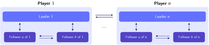
Figure 1: A schematic representation of a NASP with $n$ players with $2$ followers each. The vertical arrows represent sequential “Stackelberg” interactions, while the horizontal ones are simultaneous “Nash” interactions.

The Game.

This paper introduces a class of games capturing a hierarchical system of sequential and simultaneous interactions among decision-makers as shown in Figure 1. Specifically, we study a class of complete-information, simultaneous and non-cooperative “Nash” games among “Stackelberg” players (NASPs) where:

1. There are $n$ first-mover players called the leaders, each of which has a set of lower-level agents called the followers. Leaders and followers hierarchically decide their strategies by solving optimization problems, and the parameters of such problems are common information.

2. Each follower is associated with a unique leader and decides by optimizing a parametrized convex quadratic function over a set of linear constraints. Precisely, each follower solves an optimization problem where the objective function and the feasible region are parametrized in the decision variables of its leader. Furthermore, each follower simultaneously interacts with the other followers associated with the same leader; therefore, its objective function is also parametrized in the other followers’ variables.

3. Each leader optimizes an objective function that is linear in its variables and parametrized in the other leaders’ variables through bilinear terms. Furthermore, each leader’s optimization problem is constrained by linear inequalities involving the leader’s and its followers’ variables.

4. The leaders act simultaneously and non-cooperatively at the upper level. Given the decisions of each leader, its followers play simultaneously and non-cooperatively at the lower level. Specifically, each follower interacts with the followers having the same leader and does not interact with the other leaders’ followers.

Whenever we embed the followers’ optimization problems inside their associated leader’s optimization problem, we obtain a so-called Stackelberg game. In other words, a Stackelberg game is an optimization problem maximizing the leader’s objective subject to its constraints and the optimality of its followers’ optimization problems. Since the latter can be equivalently formulated through each follower’s Karush–Kuhn–Tucker conditions ($KKT$), we can express each Stackelberg game as a non-convex optimization problem that embeds the hierarchical interactions among a leader and its followers. As a consequence, we define a NASP as a simultaneous game where each player solves a Stackelberg game.

Remark 1.

We refer to the Stackelberg games associated with each leader as the players. The feasible set of a leader is defined by the linear inequalities directly associated with the leader’s optimization problem. In contrast, the feasible set of a player is defined by the leader’s constraints and the optimality of the followers’ optimization problems (or, equivalently, the $KKT$ conditions).

NASPs fall in the category of Equilibrium Problems with Equilibrium Constraints (EPECs), a class of problems possessing several applications in energy and pricing contexts [39, 45, 59, 58]. The Stackelberg leaders may represent first-mover decision-makers, for instance, governmental agencies and regulatory bodies; their followers may represent market players simultaneously optimizing their benefits under their leader’s regulations. In Example 1, we showcase a simple NASP.

Example 1.

Consider a NASP with $2$ players, the Latin player and the Greek player, having $2$ followers and $1$ follower, respectively. Let $w$ be the variables of the Latin leader and $y^{1}$ and $y^{2}$ be the variables of its followers. Let $\xi$ be the Greek leader’s variables and $\chi$ be the variables of its follower. Given $\xi,\chi$ as parameters, the Latin player solves the Stackelberg game

$$\min_{w,y}\quad\quad c^{\top}\left(\begin{array}[]{c}w\\ y\end{array}\right)+\left(C\left(\begin{array}[]{c}\xi\\ \chi\end{array}\right)\right)^{\top}\left(\begin{array}[]{c}w\\ y\end{array}\right)$$ (1g)

s.t. $$Aw+B\left(\begin{array}[]{c}y^{1}\\ y^{2}\end{array}\right)\quad\leq\quad b,$$ (1j)

$$y^{1}\quad\in\quad\arg\min_{y^{1}}\left\{\frac{1}{2}(y^{1})^{\top}Fy^{1}+f^{\top}y^{1}+(Gy^{2}+Hw)^{\top}y^{1}:Lw+Ny^{1}\leq d\right\},$$ (1k)

$$y^{2}\quad\in\quad\arg\min_{y^{2}}\left\{\frac{1}{2}(y^{2})^{\top}Oy^{2}+h^{\top}y^{2}+(Py^{1}+Qw)^{\top}y^{2}:Rw+Sy^{2}\leq e\right\}.$$ (1l)

Similarly, given $$w,y=(y^{1},y^{2})$$ as parameters, the Greek player solves the Stackelberg game

$$\min_{\xi,\chi}\quad\quad \alpha^{\top}\left(\begin{array}[]{c}\xi\\ \chi\end{array}\right)+\left(\Gamma\left(\begin{array}[]{c}w\\ y\end{array}\right)\right)^{\top}\left(\begin{array}[]{c}\xi\\ \chi\end{array}\right)\qquad\qquad\qquad\qquad\qquad\qquad\qquad\quad$$ (1s)

s.t. $$\Phi\xi+\Psi\chi\quad\leq\quad\beta,$$ (1t)

$$\chi\quad\in\quad\arg\min_{\chi}\left\{\frac{1}{2}\chi^{\top}\Delta\chi+\Phi^{\top}\chi+(\Upsilon\xi)^{\top}\chi:\Pi\xi+\Omega\chi\leq\gamma\right\}.$$ (1u)

In the above NASP formulation, $F$, $O$ and $\Delta$ are symmetric positive semi-definite matrices, $c$, $b$, $d$, $e$, $f$, $h$, $\alpha$, $\beta$, $\gamma$ are parameter vectors of appropriate dimensions. The remaining objects are matrices of appropriate dimensions. The objective function of each player is parametrized with respect to the variables of the other players. The objective function of each follower is parametrized in (i.) its leader’s variables, and (ii.) the variables of the other followers associated with its leader.

Applications.

NASPs provide a flexible modeling framework for many economic markets where several regulatory bodies interact and hierarchically regulate a set of lower-level economic agents. We outline three different applications related to energy, vaccine production, and insurance markets. First, the framework of NASPs is mainly motivated by international energy markets with climate change-aware regulatory authorities and profit-maximizing energy producers. In this context, each energy producer, i.e., each follower, competes in its respective domestic market regulated by a single regulatory agency through taxes (e.g., a carbon tax) and production caps. Each regulatory agency, i.e., each leader, negotiates environmental agreements for trading energy and interacts with other regulatory authorities. As we will show, the NASP abstraction practically captures the structure of such energy markets and it provides a general framework to derive practical insights into the effectiveness of environmental and regulatory initiatives. Recently, Anjos et al. [3] studied a complex multinational carbon-credit system for the energy market exploiting the models and the algorithms available in this work. Second, NASPs can model complex drug trade markets. For instance, the COVID-19 vaccine production and exchange posed a severe threat to the world’s immunization programs during the pandemic. Some experts warned of vaccine nationalism [68], a phenomenon encompassing the strict export and import regulations several countries have imposed on vaccines and the raw materials required for their production [37, 10, 9]. In this context, countries would act as leaders by regulating the trade of vaccines and providing incentives to domestic vaccine producers that would serve as followers. The leaders’ objective functions could model several tactical requirements; for instance, they can prioritize the production of doses reserved for vulnerable classes of the population or incentivize exports to neighboring countries. Third, NASPs can model several dynamics associated with insurance markets, specifically, hierarchical multi-insurer games embedding re-insurance mechanisms [41, 19]. Companies acting as followers contract insurance services to protect their operations from disruptions, e.g., cyberattacks. The insurers, acting as leaders, sell insurance products to their followers. The insurers may also mutually protect their portfolios to avoid losses due to large-scale disruptions, for instance, natural disasters.

Primary Contributions

We introduce NASPs, a class of games encompassing a series of hierarchical and simultaneous interactions among several decision-makers solving optimization problems. While the solution concept for each Stackelberg game is the Stackelberg equilibrium, namely, a solution where the followers’ decisions are optimal given the leader’s decisions, we employ the Nash equilibrium as the standard solution concept for NASPs. In a Nash equilibrium, players are mutually optimal and cannot unilaterally deviate from the equilibrium without diminishing their benefits, i.e., decreasing their objective function value. We distinguish between Pure-Strategy Nash equilibria (PNEs) and Mixed-Strategy Nash Equilibria (MNEs); players employ deterministic strategies in the former, while in the latter, players randomize over their strategies. Unless otherwise stated, we focus on the more general concept of MNE. We provide several theoretical, algorithmic, and practical contributions concerning the existence, computation, and interpretation of Nash equilibria in NASPs. Precisely:

1. We characterize the hardness of deciding whether a given instance of NASP admits a Nash equilibrium or not as a $\Sigma^{p}_{2}$-hard decision problem (Section 4). In other words, as long as $\mathcal{N}\mathcal{P}\neq\Sigma_{2}^{p}$, it is impossible to represent this problem as an integer program of polynomial size [69]. Under some mild conditions, we show that some NASP instances always admit an MNE (Corollary 1).

2. We provide the first exact and computationally-efficient algorithm to compute and select Nash equilibria in NASPs (Section 5). In contrast to the previous literature, our algorithm is exact and terminates with either a Nash equilibrium or a proof of its non-existence. We introduce two additional variants of our algorithm: a variant built upon an iterative inner-approximation scheme and a variant computing PNEs (Section 6). Our algorithms are based on the insight that any NASP possesses an equivalent convex representation (Theorems 4 and 3).

3. We apply NASPs to model international energy markets where climate-change aware regulators oversee the operations of profit-driven energy producers (Section 7). We provide a detailed computational analysis of the performance of our algorithms on a set of synthetic energy-market instances. Furthermore, by combining real-world data and our models, we derive informative yet counterintuitive managerial insights from the MNEs. We also provide an analysis of the Chilean-Argentinean energy market and derive some insights for the policymakers.

We organize the manuscript as follows. In Section 2, we provide a literature review, while in Section 3, we introduce the background definitions. In Section 4, we present an overview of the computational complexity results. In Section 5, we present and characterize the algorithm to find equilibria in NASPs. In Section 6, we introduce an inner approximation algorithm and an algorithm to exclusively compute PNEs. In Section 7, we present the energy model, the computational tests, and the managerial insights. Finally, in Section 8, we provide some concluding remarks.

2 Literature Review

Nash [55, 54] introduced the concept of Nash Equilibrium in the context of finite games, i.e., games with a finite number of players and strategies. Nash proved that if the game is finite, there always exists an MNE. Within the optimization community, games expressed through the parametrized optimization problems associated with the players are often known as Nash equilibrium problems or Nash games. The Nash equilibrium concept has dramatically changed several scientific fields due to its flexibility and interpretability. Several authors employed Nash equilibria to capture the outcome of structured interactions of players solving optimization problems. For instance, gas market modeling [30, 35, 62, 36, 44, 29, 66], cross-border kidney exchange models [14, 13], competitive lot-sizing models [51, 16], knapsack and network-formation games [27, 17], and fixed-charge transportation models [61] employed the concept of Nash equilibrium.

In contrast to simultaneous games, sequential games partition the set of players into different groups, each playing in a predetermined round. When there are two rounds, the game is known as a Stackelberg game [67], with the first-round players being the leaders and the second-round players being the followers. In the optimization literature, Stackelberg games where players solve optimization problems are related to bilevel programming [21], and their applications span several domains. For instance, Bard et al. [6, 7] modeled taxation strategies in the context of biofuel production, Brotcorne et al. [11], Labbé and Violin [49], Grimm et al. [42] modeled bilevel pricing problems, and Hobbs et al. [43], Gabriel and Leuthold [38], Feijoo and Das [34] modeled pricing and environmental policies for energy markets, with power generators being leaders and network operators being followers.

Algorithms.

When multiple Stackelberg leaders, each possibly having multiple followers, interact, the game belongs to the family of EPECs. Their application in economics often involves a multi-leader, multi-follower game [57]. Several authors employed EPECs to represent economic markets involving several decision-makers. Sherali [63] introduced EPECs where both leaders and followers produce a homogeneous commodity, and Ralph and Smeers [59] and Hu and Ralph [45] studied the existence of PNEs in some specialized classes of EPECs arising in electricity markets. DeMiguel and Xu [24] crafted the concept of stochastic multi-leader Stackelberg-Nash-Cournot equilibrium for a particular form of investment-production interactions. Regarding methodological contributions, Gabriel et al. [39] provided an iterative algorithm to compute PNEs in a restricted class of EPECs where followers from distinct leaders interact. Leyffer and Munson [50] introduced an alternative solution concept based on a nonlinear programming reformulation. Kulkarni and Shanbhag [47, 48] analyzed EPECs with shared constraints and introduced solution concepts and algorithms when the players’ objective functions fulfill specific properties. Recently, Devine and Siddiqui [26] introduced an EPEC model for electricity markets with price-making firms with market power and price-taking firms. In contrast to this work, the previous works on EPECs either: (i.) proposed algorithms to exclusively compute PNEs, or (ii.) focused on weaker notions of equilibria. To the best of our knowledge, this is the first work providing an algorithm to compute exact MNEs for the large class of EPECs that NASPs represent.

Complexity and Equilibria.

The two paramount issues concerning Nash equilibria are existence, namely, determining when at least one equilibrium exists, and computation, namely, devising efficient algorithms to compute equilibria. The original proof of existence from Nash [55, 54] holds only for finite games, is non-constructive, and provides no methodology for computing or analytically constructing equilibria. Indeed, even if an equilibrium always exists, as in finite games or games with specific structures [60, 23], the problem of computing it is often not trivial, even in simple $2$-player cases [20]. Furthermore, many variations of the decision version of the equilibrium problem are $\mathcal{NP}$-complete [40], for instance, the problem of determining an equilibrium with specific properties. In general, an equilibrium may not even exist when players solve parametrized non-convex problems. For example, when players solve parametrized integer programs, Carvalho et al. [15, 18] proved that deciding if a Nash equilibrium exists is $\Sigma^{p}_{2}$-hard.

In the context of Stackelberg games with a single leader, however, the standard solution concept is the one of Stackelberg equilibrium. The seminal work of Jeroslow [46] proved that the complexity of determining if a sequential game admits an equilibrium rises one level up in the polynomial hierarchy for every additional round.

3 Definitions and Background

This section provides the basic notations and definitions we employ throughout the paper. As a standard notation in game theory, let the operator $\left(\cdot\right)^{-i}$ denote $\left(\cdot\right)$ except $i$. For any pair of vectors $\nu\in\mathbb{R}^{t}$ and $\tau\in\mathbb{R}^{t}$, let $\nu\perp\tau$ be equivalent to $\nu^{\top}\tau=0$. Given $M\in\mathbb{R}^{t\times t}$ and $q\in\mathbb{R}^{t}$, the linear complementarity problem (LCP) is the problem of finding, if any, a vector $\nu\in\mathbb{R}^{t}$ such that $0\leq\nu\perp(M\nu+q)\geq 0$ [33, 32, 22]. We say that the optimization problem in $y\in\mathbb{R}^{n_{f}}$ has a simple parameterization with respect to $x\in\mathbb{R}^{n_{\ell}}$ if the problem is in the form of $\min_{y\in\mathbb{R}^{n_{f}}}\{f(y)+(Cx)^{\top}y:y\in\mathscr{F},Ax+By\leq b\}$, where $C$, $A$, $B$, $b$ are matrices and vectors of appropriate dimensions, $\mathscr{F}\subseteq\mathbb{R}^{n_{f}}$, and $f:\mathbb{R}^{n_{f}}\to\mathbb{R}$.

3.1 Simultaneous Games

Definition 1 (Simultaneous “Nash” Game).

A simultaneous game $P$ among $n$ players is a finite tuple of optimization problems $P=\left(P^{1},\dots,P^{n}\right)$, where each player $i$ solves $P^{i}=P^{i}(x^{i},x^{-i})=\min_{x^{i}\in\mathbb{R}^{n_{i}}}\{f^{i}(x^{i},x^{-i}):x^{i}\in\mathscr{F}^{i}\}$ with $f^{i}$ and $\mathscr{F}^{i}$ being the objective function and the feasible set of $i$, respectively. The game has complete information if every player knows $\mathscr{F}^{1},\dots,\mathscr{F}^{n}$ and $f^{1},\dots,f^{n}$.

Depending on the structure of each optimization problem $P^{i}$, we characterize the game as (i) simpleif, for every player $i$, $f^{i}(x^{i},x^{-i})=\frac{1}{2}(x^{i})^{\top}Q^{i}x^{i}+(c^{i})^{\top}x^{i}+(C^{i}x^{-i})^{\top}x^{i}$ where $Q^{i}$ is a positive semi-definite matrix, and $c^{i}$ and $C^{i}$ are a vector and a matrix of appropriate dimensions, respectively, or (ii) linear, if the game is simple and $Q^{i}=0$ for all $i$, or (iii) facile, if the game is simple and $\mathscr{F}^{i}$ is a polyhedron for any $i$. Furthermore, for any player $i$, we call any $x^{i}\in\mathscr{F}^{i}$ a pure strategy. If a player randomizes over its pure strategies, we call the resulting strategy mixed. Formally, a mixed strategy $\sigma^{i}$ for player $i$ is a probability distribution over $\mathscr{F}^{i}$.

Definition 2 (Nash equilibrium).

Given a simultaneous game $P$, $\sigma=(\sigma^{1},\dots,\sigma^{n})$ is an MNE for $P$ if $\mathbb{E}_{X\sim\sigma}\left[f^{i}(X^{i},X^{-i})\right]\leq\mathbb{E}_{X^{-i}\sim\sigma^{-i}}\left[f^{i}(\widetilde{x}^{i},X^{-i})\right]$ for any player $i$ and for any $\widetilde{x}^{i}\in\mathscr{F}^{i}$. If $\sigma^{i}$ has a singleton support for any $i$, then $\sigma$ is a PNE.

Intuitively, Definition 2 states that in a Nash equilibrium $\sigma=(\sigma^{1},\dots,\sigma^{n})$, no player $i$ can unilaterally deviate from $\sigma^{i}$ to any other strategy without increasing the expectation of its objective function value, i.e., without being strictly worse off compared to the equilibrium strategy.

Whenever $P$ is a facile Nash game, each player’s problem is convex in its variables. Therefore, the set of points $x=(x^{1},\dots,x^{n})$ concurrently satisfying the $KKT$ conditions of every problem $P^{i}$ form the set of PNEs for $P$. Equivalently, these conditions could be reformulated as an LCP involving a matrix $M$ and a vector $q$ such that every solution to $0\leq x\perp(Mx+q)\geq 0$ is a PNE for $P$ and every PNE of $P$ solves the LCP [22].

3.2 Stackelberg Games

In contrast to simultaneous games, the players of Stackelberg games play in two rounds [12]. Let $w\in\mathbb{R}^{n_{\ell}}$ be the leader’s variables. After the leader plays, its followers compete in a simultaneous game parametrized in the leader’s variables $w$. Specifically, in this paper, the followers play a simultaneous game $P(w)$ that has a simple parameterization with respect to $w$, i.e., each problem $P^{1}(w),\dots,P^{n}(w)$ has a simple parameterization with respect to $w$.

Definition 3 (Stackelberg game).

Let $P(w)$ be a simultaneous game with a simple parametrization with respect to $w\in\mathbb{R}^{n_{\ell}}$, $\operatorname{SOL}(P(w))$ be its solution set, $f$ be a function such that $f:\mathbb{R}^{n_{\ell}+n_{f}}\to\mathbb{R}$, and $\mathcal{S}\subseteq\mathbb{R}^{n_{\ell}+n_{f}}$. A Stackelberg game $S$ is the optimization problem $\displaystyle S=\min_{w\in\mathbb{R}^{n_{\ell}},y\in\mathbb{R}^{n_{f}}}\{f(w,y):(w,y)\in\mathcal{S},\;y\in\operatorname{SOL}(P(w))\}$.

If $P(w)$ is a facile simultaneous game with a simple parameterization with respect to the leader’s variables $w$, $\mathcal{S}$ is a polyhedron, and $f(w,y)$ is a linear function, we say $S$ is a simple Stackelberg game. From a game-theory perspective, the solution of a Stackelberg game is a so-called subgame perfect Nash equilibrium. We remark that Definition 3 implies that the Stackelberg game is optimistic, i.e., if $P(w)$ has more than one solution, then the followers collectively select the solution $y\in\operatorname{SOL}(P(w))$ maximizing the leader’s objective function [25]. The optimistic assumption may be quite restrictive when $|\operatorname{SOL}(P(w))|>1$, since it exposes the issue of equilibria selection for the followers’ game. However, it also has a strong economic interpretation. The leader can, in fact, persuade followers to play a favorable solution by transferring utility, i.e., by paying followers an arbitrarily small value. Whenever the followers solve strictly convex quadratic programs, as in our application in Section 7, the optimistic assumption is not restrictive since there is always a unique followers’ equilibrium (i.e., $|\operatorname{SOL}(P(w))|=1$). Recently, Basu et al. [8] provided an extended formulation for the feasible region of a simple Stackelberg game. Specifically, the authors proved that the feasible region $\{(w,y)\in\mathcal{S},\;y\in\operatorname{SOL}(P(w))\}$ of a simple Stackelberg game is the union of finitely many polyhedra. We will later employ this result to prove that the convex hull of the union of these polyhedra is the space of mixed strategies for each NASP player.

3.3 NASPs

Combining the previous definitions, a NASP is a simultaneous game with complete information where each player solves a simple parametrized Stackelberg game.

Definition 4 (NASP).

A NASP $N=(S^{1},\dots,S^{n})$ is a complete-information simultaneous game among $n$ players, where each player $i$ solves the simple Stackelberg game $S^{i}(x^{i},x^{-i})=\min_{\begin{subarray}{c}x^{i}\in\mathbb{R}^{n_{\ell}+n_{f}}\end{subarray}}\{(c^{i})^{\top}x^{i}+(C^{i}x^{-i})^{\top}x^{i}:x^{i}\in\mathscr{F}^{i}\}$ with $\mathscr{F}^{i}:=\{x^{i}=(w^{i},y^{i}):x^{i}\in\mathcal{S}^{i},\;y^{i}\in\operatorname{SOL}(P(w^{i}))\}$, and $\mathcal{S}^{i}$ being a polyhedron.

In Definition 4, we let $x^{i}\in\mathbb{R}^{n_{\ell}+n_{f}}$ be a joint representation of the leader’s and the followers’ variables for the $i$-th NASP player. We refer to $\mathscr{F}^{i}$ as the $i$-th player feasible region, and we say that $\mathscr{F}^{i}$ is bounded if $\mathcal{S}^{i}$ is a polytope and $\operatorname{SOL}(P(w^{i})$ is finite.

Remark 2.

The Nash equilibrium of Definition 2 directly applies to the NASPs of Definition 4. We remark that, based on our previous definitions, we only consider NASPs where each Stackelberg game fulfills the optimistic assumptions. Therefore, when we claim a NASP does not have an MNE, we claim that no MNE exists when each leader’s followers select the most favorable equilibrium for the leader. If there is no MNE satisfying the optimistic assumption, there might exist an MNE where the players do not fulfill such assumption.

4 Hardness of Finding a Nash Equilibrium

We characterize the computational complexity associated with deciding whether a NASP admits an MNE or not as $\Sigma^{p}_{2}$-hard. This result holds even for the simplest of NASPs called a trivial NASP $N=(S^{1},S^{2})$. In the latter, two leaders have a single follower each, and each follower solves a parametrized linear problem. We formalize our results in Theorem 1, Corollary 1, and Theorem 2.

Theorem 1.

It is $\Sigma^{p}_{2}$-hard to decide if a trivial NASP has a PNE.

Corollary 1.

If each player’s feasible set in a NASP is bounded, an MNE exists.

Theorem 2.

It is $\Sigma^{p}_{2}$-hard to decide if a trivial NASP has an MNE.

Proof of Theorem 1..

Carvalho et al. [15, Theorem 2.1] showed that deciding if a PNE exists is $\Sigma^{p}_{2}$-hard in two-player simultaneous games where (i.) each player solves a binary integer program with bounded variables, and (ii.) $f^{i}$ is linear in $x^{i}$ and parametrized in $x^{-i}$. We employ this result by formulating the Stackelberg game associated with each player as a parametrized integer program. First, we can employ the reformulation proposed in Basu et al. [8]; it requires that the parametrized integer program has a bounded feasible region and is thus compatible with (i.). Second, we can employ the reformulation proposed in Audet et al. [4]; it requires that all integer variables are binary, and thus it is also compatible with (i.). Since the objective of each player $i$ is linear in $x^{i}$, the result of Carvalho et al. [15] extends to trivial NASPs. ∎

Under an assumption of boundedness, we also show that a trivial NASP always admits an MNE.

Proof of Corollary 1..

Let $\mathscr{F}^{i}$ be bounded for each player $i$. If $f^{i}$ is linear in $x^{i}$, there always exists an optimal solution that is an extreme point of $\operatorname{conv}(\mathscr{F}^{i})$. Since the feasible set $\mathscr{F}^{i}$ of each simple Stackelberg game is a union of polyhedra [8], $\operatorname{conv}(\mathscr{F}^{i})$ is a polyhedron. Furthermore, since $\mathscr{F}^{i}$ is bounded, $\operatorname{conv}(\mathscr{F}^{i})$ is precisely a polytope, and the strategies of player $i$ are the finitely many extreme points of $\operatorname{conv}(\mathscr{F}^{i})$. Since each player has finitely many strategies, the game is finite, and it always admits an MNE [54]. ∎

We complement the previous result with Theorem 2, where we show that if at least one player’s feasible region is not bounded, deciding on the existence of an MNE is $\Sigma^{p}_{2}$-hard. In contrast to the proof of Theorem 1, we could not apply any of the result of Carvalho et al. [18, 15] since the reformulated players’ integer programs: (i.) are not bounded, preventing us from applying the reduction of Basu et al. [8], and (ii.) employ general integer variables as opposed to binary variables, preventing us from using the reduction of Audet et al. [4]. Based on the one of Carvalho et al. [18, 15], we provide a novel proof that reduces the problem of computing an MNE in a NASP to the Subset Sum Interval (SSI) problem. While the full proof and its associated claims are available in the electronic companion, we provide a proof sketch below.

Definition 5 (SSI).

Given $q_{1},\ldots,q_{k},p,t,k\in\mathbb{Z}_{+}$ and $\log_{2}(t-p)\leq k$, does there exist an integer $s\in\mathbb{Z}$ with $p\leq s<t$, such that, for all $I\subseteq\{1,2,\dots,k\}$, then $\sum_{i\in I}q_{i}\neq s$?

The term $t-p$ can be a power of $2$, and the SSI would then asks if there exists an $r\in\mathbb{Z}_{+}$ such that $2^{r}=t-p$. Eggermont and Woeginger [28] proved that, given $r\in\mathbb{Z}_{+}$ such that $t-p=2^{r}$, the problem is $\Sigma^{p}_{2}$-complete.

Proof Sketch of Theorem 2..

We reduce SSI to the problem of deciding on the existence of an MNE for a trivial NASP. Let $Q=\sum_{i=1}^{k}q_{i}$. We explicitly formulate the Stackelberg games associated with each player of a trivial NASP and denote them as the Latin and the Greek game, respectively. Let $w$ be the Latin leader’s decision variables, and let $y$ be its follower variables. Similarly, let $\xi$ be the Greek’s leader variables and $\chi$ its follower ones. The Latin player solves the problem

$$\max_{\begin{subarray}{c}w_{0},\dots,w_{k+3r+1}\in\mathbb{R}\\ y_{0},\dots,y_{k}\in\mathbb{R}\end{subarray}}\quad\quad \frac{w_{0}}{2}+\sum_{i=1}^{k}q_{i}w_{i}+2(Q+1)\xi_{r+1}w_{k+3r+1}$$

$$\qquad-(Q+1)\left(\sum_{i=1}^{r}2^{i-1}w_{k+i}+pw_{k+3r+1}\right)$$ (2a)

$$\text{s.t.}\quad w_{i}\quad \geq\quad 0,\quad y_{i}\quad\geq\quad 0,\quad w_{i}\quad\leq\quad 1 \forall\,i=0,\dots,k,$$ (2b)

$$w_{k+3r+1}\quad =\quad w_{k+2r+i} \forall\,i=1,\dots,r,$$ (2c)

$$w_{k+3r+1}\quad =\quad p+\sum_{i=1}^{r}2^{i-1}w_{k+r+i},$$ (2d)

$$\frac{w_{0}}{2}+\sum_{i=1}^{k}q_{i}w_{i}\quad \leq\quad w_{k+3r+1},$$ (2e)

$$(w_{k+i},w_{k+r+i},w_{k+2r+i})\quad \in\quad\Big{\{}(h,y,w)\in\mathbb{R}^{3}_{+}:\left\{h=w,y=1\right\}\cup\left\{h=y=0\right\}\Big{\}} \forall\,i=1,\dots,r,$$ (2f)

$$\left(y_{0},\dots,y_{k}\right)\quad \in\quad\arg\min_{y}\left\{\sum_{i=0}^{k}y_{i}:\begin{array}[]{l}y_{i}\geq-w_{i}\\ y_{i}\geq w_{i}-1\end{array}\forall\,i=0,\dots,k\right\}.$$ (2i)

The Greek player solves the problem

$$\max_{\begin{subarray}{c}\xi_{0},\dots,\xi_{r+1}\in\mathbb{R}\\ \chi_{1},\dots,\chi_{r}\in\mathbb{R}\end{subarray}}\quad\quad (1-w_{0})\xi_{0}$$ (2j)

$$\text{s.t.}\quad\xi_{i}\quad \geq\quad 0,\quad\chi_{i}\quad\geq\quad 0,\quad\xi_{i}\quad\leq\quad 1 \qquad\forall\,i=1,\dots,r,$$ (2k)

$$p+\sum_{i=1}^{r}2^{i-1}\xi_{i}\quad =\quad\xi_{r+1},$$ (2l)

$$\left(\chi_{1},\dots,\chi_{r}\right)\quad \in\quad\arg\min_{\chi}\left\{\sum_{i=1}^{r}\chi_{i}:\begin{array}[]{l}\chi_{i}\geq-\xi_{i}\\ \chi_{i}\geq\xi_{i}-1\end{array}\forall\,i=0,\dots,r\right\}.$$ (2o)

We show that the NASP in 2 has an MNE if and only if the corresponding SSI problem has an answer YES. First, we prove that the formulation ensures that $w_{0},\ldots,w_{k}$ and $\xi_{0},\ldots,\xi_{r}$ are binary (Claim 2). Considering the Greek player, if $w_{0}=1$, no matter what the Greek player does, its objective function value necessarily equals $0$, the smallest value it can take. We construct an MNE in this case. If $w_{0}=0$, then $\xi_{0}$ can be arbitrarily large, and there always exists a profitable unilateral deviation for the Greek player. Therefore, the problem of checking the existence of an MNE collapses to the problem of determining whether the Greek player can induce the Latin player to choose $w_{0}=0$ or not. By observing the last two terms in the Latin leader’s objective function, we prove that the Latin player plays optimally by always choosing $w_{k+3r+1}=\xi_{r+1}$. Indeed, if $w_{k+3r+1}\neq\xi_{r+1}$, the Latin player acts suboptimally (Claim 5).

On the one hand, if the SSI instance is a YES instance (i.e., it admits a solution), then let $\xi_{r+1}=s$. Since $s$ cannot be represented as a subset-sum, the Latin player can never ensure that 2e is satisfied with equality. Even if $w_{0}=1$, it only adds $0.5$ to the LHS of 2e. However, the Latin player would be better off by selecting $w_{0}=1$, as $w_{0}$ appears in the Latin leader’s objective and can improve the objective function’s value by $0.5$.

On the other hand, if the SSI instance is a $NO$ instance, no matter what value the Greek player assigns to $\xi_{r+1}=w_{k+3r+1}$, the Latin player will always ensure that 2e is satisfied with equality by choosing $w_{0}=0$. Choosing $w_{0}=1$ is not optimal for the Latin player since it would improve the objective only by $0.5$ while enforcing $w_{0}=0$ would improve the objective at least by $1$. Therefore, enforcing $w_{0}=0$ is optimal for the Latin player, and the Greek player will never have a profitable deviation from any feasible strategy. ∎

5 The Enumeration Algorithm

Although we proved that deciding on the existence of Nash equilibria is $\Sigma^{p}_{2}$-hard, in this section, we present an effective and exact algorithm to compute MNEs. Our algorithmic scheme exploits the structure of the (non-convex) feasible region $\mathscr{F}^{i}=\{x^{i}=(w^{i},y^{i}):x^{i}\in\mathcal{S}^{i},\;y^{i}\in\operatorname{SOL}(P(w^{i}))\}$ of each player $i$. While $\mathcal{S}^{i}$ is a polyhedron, $\operatorname{SOL}(P(w^{i}))$ is the parametrized set of solutions for the followers’ game. We also recall that $\operatorname{SOL}(P(w^{i}))$ is the set of points satisfying all the $KKT$ conditions associated with the followers’ optimization problems. Assuming such $KKT$ conditions are expressed as complementarity conditions, then

$$\mathscr{F}^{i}=\{x^{i}=(w^{i},y^{i}):x^{i}\in\mathcal{S}^{i},\;z^{i}=M^{i}x^{i}+q^{i},\;0\leq x^{i}_{j}\perp z^{i}_{j}\geq 0\;\;\;\forall\,j\in\mathcal{C}^{i}\}.$$ (3)

In the above reformulation, we let $\mathcal{C}^{i}$ be the set of indices for the complementarity conditions $0\leq x^{i}_{j}\perp z^{i}_{j}\geq 0$ describing $\operatorname{SOL}(P(w^{i}))$, and $q^{i}$ and $M^{i}$ be a vector and a matrix of appropriate dimensions, respectively. The set $\mathscr{F}^{i}$ also has an equivalent representation as the union of finitely many polyhedra. Let $\mathcal{O}^{i}=\{x^{i}:x^{i}\in\mathcal{S}^{i},\;z^{i}=M^{i}x^{i}+q^{i},\;x^{i}_{j}\geq 0,\;z^{i}_{j}\geq 0\;\;\;\forall\,j\in\mathcal{C}^{i}\}$ be the polyhedral relaxation of $\mathscr{F}^{i}$. For every player $i$, the finitely many polyhedra whose union is $\mathscr{F}^{i}$ are given by the complementarity polyhedra of Definition 6.

Definition 6 (Complementarity Polyhedron).

Given a player $i$ and a binary vector $\theta^{i}\in\{0,1\}^{|\mathcal{C}^{i}|}$, the complementarity polyhedron corresponding to $\theta^{i}$ is

$$\mathscr{P}^{i}(\theta^{i})=\{(x^{i},z^{i})\in\mathcal{O}^{i}:x^{i}_{j}\leq 0\;\;\forall\;j:\theta^{i}_{j}=0\}\cap\{(x^{i},z^{i})\in\mathcal{O}^{i}:z^{i}_{j}\leq 0\;\;\forall\;j:\theta^{i}_{j}=1\}.$$

In other words, for any player $i$, $\theta^{i}$ identifies whether the $j$-th complementarity conditions is active ($x^{i}_{j}\leq 0$) or not ($z^{i}_{j}\leq 0$) in the polyhedron $\mathscr{P}^{i}(\theta^{i})$. Therefore, $\mathscr{F}^{i}$ is the finite union of all the complementarity polyhedra, i.e., $\mathscr{F}^{i}=\bigcup_{\theta^{i}\in\{0,1\}^{|\mathcal{C}^{i}|}}\mathscr{P}^{i}(\theta^{i})$. Let $k^{i}$ be the number of the non-empty complementarity polyhedra associated with player $i$. The core idea behind our algorithm is to reformulate the NASP by letting each player select its strategies from $\operatorname{cl}\operatorname{conv}(\mathscr{F}^{i})$, i.e., the closure of the convex hull of $\mathscr{F}^{i}$, instead of $\mathscr{F}^{i}$. In other words, we convexify the NASP by letting players select their strategies from $\operatorname{cl}\operatorname{conv}(\mathscr{F}^{i})$. We prove that any PNE of the convexified NASP maps to an equivalent MNE in the original non-convex NASP. In practice, this idea requires, for each player $i$, the explicit enumeration of the $k^{i}$ complementarity polyhedra and the computation of the closure of their convex hull. We will employ the result of Balas [5] to compute the latter.

Theorem 3 (Balas [5]).

Given $k$ polyhedra $K_{j}=\{x\in\mathbb{R}^{n}:A_{j}x\leq b_{j}\}$ for $j=1,\dots k$, then $\operatorname{cl}\operatorname{conv}(\bigcup_{j=1}^{k}K_{j})=\{x\in\mathbb{R}^{n}:\exists(x_{1},\ldots,x_{k},\delta)\in(\mathbb{R}^{n})^{k}\times\mathbb{R}^{k}:A_{j}x_{j}\leq\delta_{j}b_{j},\;\sum_{w=1}^{k}x_{w}=x,\;\sum_{w=1}^{k}\delta_{w}=1,\;\delta_{j}\geq 0,\;\forall j=1,\dots,k\}$.

The last ingredient of our algorithm is the result of Stein et al. [65, Theorem 2.7] for separable simultaneous games, i.e., simultaneous games where $f^{i}(x^{i},x^{-i})$ is a separable polynomial for every player $i$. In a separable simultaneous game, Stein et al. [65] proved that every mixed strategy $\sigma^{i}$ of player $i$ has either finite support or a finite support equivalent. Since NASPs are indeed separable simultaneous games, we restrict our attention to MNEs where the players randomize over a finite number (precisely, at most $k^{i}$) of pure strategies.

The Enumeration Algorithm.

We formalize our enumeration scheme in Algorithm 1. Given a NASP instance $N=(S^{1},\dots,S^{n})$, the algorithm returns either an MNE for $N$ or a proof of its non-existence, i.e., a no certificate. Algorithm 1 exploits the equivalent convex representation of $N$, where each player’s feasible region $\mathscr{F}^{i}$ is replaced by $\widetilde{\mathscr{F}}^{i}:=\operatorname{cl}\operatorname{conv}(\mathscr{F}^{i})$. In Algorithm 1, the algorithm retrieves the sets $\widetilde{\mathscr{F}}^{i}$ by enumerating the $k^{i}$ complementarity polyhedra and computing the closure of their convex hull through the extended formulation of Theorem 3. In Algorithm 1, the algorithm reformulates $N$ into the equivalent simultaneous game $\widetilde{N}$, where each player $i$ solves $\widetilde{S}^{i}:=\min_{x^{i}\in\mathbb{R}^{n_{\ell}+n_{f}}}\{f^{i}(x^{i},x^{-i})=(c^{i})^{\top}x^{i}+(C^{i}x^{-i})^{\top}x^{i}:x^{i}\in\widetilde{\mathscr{F}}^{i}\}$. At this step, $\widetilde{N}$ is a facile simultaneous game, and we can formulate an LCP to determine its PNEs.

Data: A NASP instance $N=(S^{1},\ldots,S^{n})$.

Result: Either: (i.) $(\widehat{x}^{i},p^{i})$ for every $i$, or (ii.) no.

1 for $i\leftarrow 1$ to $n$ do

2       $\widetilde{\mathscr{F}}^{i}\leftarrow\operatorname{cl}\operatorname{conv}(\mathscr{F}^{i})$ by applying Theorem 3

3       $\widetilde{S}^{i}\leftarrow\min_{x^{i}\in\mathbb{R}^{n_{\ell}+n_{f}}}\{f^{i}(x^{i},x^{-i})=(c^{i})^{\top}x^{i}+(C^{i}x^{-i})^{\top}x^{i}:x^{i}\in\widetilde{\mathscr{F}}^{i}\}$

4      

5if $\exists$ a PNE $(\widetilde{x}^{1},\ldots,\widetilde{x}^{n})$ of $\widetilde{N}=(\widetilde{S}^{1},...,\widetilde{S}^{n})$  then

6       for $i\leftarrow 1$ to $n$ do

7             if $\widetilde{x}^{i}\in\mathscr{F}^{i}$ then $\exists j:\widehat{x}^{i}_{j}\leftarrow\widetilde{x}^{i}$, $p^{i}_{j}\leftarrow 1$

8             else  $\widetilde{x}^{i}=\sum_{j=1}^{k^{i}}p^{i}_{j}\widehat{x}^{i}_{j}$ for $\widehat{x}^{i}_{1},\dots,\widehat{x}^{i}_{k^{i}}\in\mathscr{F}^{i}$ with $p^{i}_{j}\geq 0$ and $\sum_{j=1}^{k^{i}}p^{i}_{j}=1$

9            

10      return ($\widehat{x}^{i}_{j}$, $p^{i}_{j}$) for each player $i=1,\dots,n$ and $j=1,...,k^{i}$

11      

12else return no

Algorithm 1 Enumeration Algorithm for NASPs

We claim that any PNE of $\widetilde{N}$ maps to an equivalent MNE in $N$. Let $\widetilde{x}=(\widetilde{x}^{1},\dots,\widetilde{x}^{n})$ be a PNE of $\widetilde{N}$. If $\widetilde{x}^{i}\in\mathscr{F}^{i}$ for each player $i$, then $i$ plays the pure strategy $\widetilde{x}^{i}$ in the MNE of $N$; therefore, $\widetilde{x}$ is necessarily a PNE for $N$ (Algorithm 1). Otherwise, if there exists a player $i$ such that $\widetilde{x}^{i}\notin\mathscr{F}^{i}$, then $\widetilde{x}^{i}\in\operatorname{cl}\operatorname{conv}(\mathscr{F}^{i})\backslash\mathscr{F}^{i}$ and we claim that $\widetilde{x}^{i}$ is equivalent to a mixed strategy (Algorithm 1). Indeed, $\widetilde{x}^{i}$ is either a convex combination of points in $\mathscr{F}^{i}$ or a limit of such points. Specifically, the points in the support of the convex combination belong to $\mathscr{F}^{i}$, i.e., they are pure strategies; the convex combination’s coefficients $p^{i}$ are the probabilities associated with each point in the support. In practice, the probabilities $p^{i}$ are precisely the values of the $\delta$ variables provided by Theorem 3. We provide a visualization of this convexification method in Figure 2. Finally, we prove the properties of Algorithm 1 in Theorem 4.

(a) Algorithm 1 of Algorithm 1: each player’s $i$ feasible region $\mathscr{F}^{i}$ is a non-convex union of finitely many polyhedra.

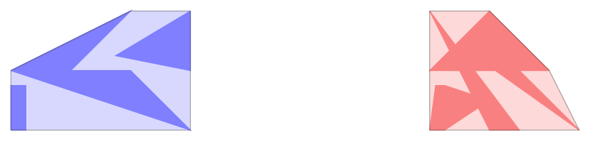
(b) Algorithm 1 of Algorithm 1: for each $i$, the algorithm computes $\operatorname{cl}\operatorname{conv}(\mathscr{F}^{i})$ via Theorem 3.

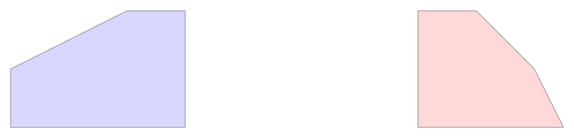
(c) Algorithm 1 of Algorithm 1: each player solves a parametrized convex problem over $\operatorname{cl}\operatorname{conv}(\mathscr{F}^{i})$.

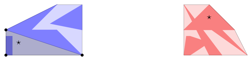
(d) Algorithms 1 and 1 of Algorithm 1: the PNE $\star$ of $\widetilde{N}$ is an MNE for $N$, since each $\widetilde{x}^{i}$ is a convex combination of strategies in $\mathscr{F}^{i}$.

Figure 2: A representation of Algorithm 1 for two players (blue and red).

Theorem 4.

Algorithm 1 terminates in a finite number of steps and returns either (i) an MNE for $N$ so that each player $i$ plays the strategy $\widehat{x}^{i}_{j}$ with probability $p^{i}_{j}$, or (ii) noif $N$ has no MNE.

Proof of Theorem 4..

The algorithm terminates in a finite number of steps since all the for loops have $n$ iterations, $k^{i}\leq 2^{\mathcal{C}^{i}}$ for any $i$, and Algorithm 1 is an LCP.

Proof of Statement (i.).

If Algorithm 1 returns $$(\widehat{x}^{i},p^{i}) \widetilde{x} \widetilde{N} f^{i} x^{i} \widetilde{x}^{i} \mathscr{F}^{i} i$$, then Algorithm 1 finds a PNE for . Since each player’s objective function is separable and linear in , is a distribution with finite support over [65]. Therefore, for every player ,

$$\mathbb{E}_{\widehat{X}\sim p}\left[\left(c^{i}+C^{i}\widehat{X}^{-i}\right)^{\top}\widehat{X}^{i}\right]\quad=\quad\sum_{j^{\prime}}\sum_{j=1}^{k_{i}}p^{-i}_{j^{\prime}}p^{i}_{j}\left(c^{i}+C^{i}\widehat{x}^{-i}_{j^{\prime}}\right)^{\top}\widehat{x}^{i}_{j}\quad=\quad\left(c^{i}+C^{i}\widetilde{x}^{-i}\right)^{\top}\widetilde{x}^{i}.$$ (4a)

Assume $$(\widehat{x}^{i},p^{i}) N i (\widehat{x}^{i},p^{i}) (\dagger\widehat{x}^{i},\dagger p^{i}) \sum_{j=1}^{k^{i}}(\dagger p^{i}_{j}\dagger\widehat{x}^{i}_{j}) i \widetilde{N} f^{i} x^{i} i \sum_{j=1}^{k^{i}}(\dagger p^{i}_{j}\dagger\widehat{x}^{i}_{j}) \widetilde{P}^{i} \widetilde{N}$$ is not an MNE for , or, equivalently, there exists player that can profitably and unilaterally deviate from to . By definition, is a pure strategy for in . By leveraging the linearity of in for any player , we can show that is also a profitable deviation for in since

$$\left(c^{i}+C^{i}\widetilde{x}^{-i}\right)^{\top}\widetilde{x}^{i} \quad=\quad\sum_{j^{\prime}}\sum_{j=1}^{k_{i}}p^{-i}_{j^{\prime}}p^{i}_{j}\left(c^{i}+C^{i}\widehat{x}^{-i}_{j^{\prime}}\right)^{\top}\left(\widehat{x}^{i}_{j}\right)$$

$$\quad\geq\quad\sum_{j^{\prime}}\sum_{j=1}^{k^{i}}p^{-i}_{j^{\prime}}\dagger p^{i}_{j}\left(c^{i}+C^{i}\widetilde{x}^{-i}_{j^{\prime}}\right)^{\top}\left(\dagger\widehat{x}^{i}_{j}\right)$$

$$\quad=\quad\left(c^{i}+C^{i}\left(\sum_{j^{\prime}}p^{-i}_{j^{\prime}}\widetilde{x}^{-i}_{j^{\prime}}\right)\right)^{\top}\left(\sum_{j=1}^{k^{i}}\dagger p^{i}_{j}\dagger\widehat{x}^{i}_{j}\right)$$

$$\quad=\quad\left(c^{i}+C^{i}\widetilde{x}^{-i}\right)^{\top}\left(\sum_{j=1}^{k^{i}}\dagger p^{i}_{j}\dagger\widehat{x}^{i}_{j}\right).$$

This last equation proves that there also exists a profitable deviation from $$(\widehat{x}^{i},p^{i}) \widetilde{N} (\widehat{x}^{i},p^{i}) \widetilde{N}$$ in , contradicting the fact is a PNE in .

Proof of Statement (ii.).

To prove this statement, we prove its contrapositive; namely, we show that if $N$ has an MNE, then Algorithm 1 obtains a PNE for $\widetilde{N}$. Let the MNE of $N$ be $(\widehat{x}^{i},p^{i})$, and let $\widetilde{x}^{i}=\sum_{j=1}^{k_{i}}p_{j}^{i}\widehat{x}^{i}_{j}$. Since $(\widetilde{x}^{1},\dots,\widetilde{x}^{n})$ is both feasible in $\widetilde{N}$ and an MNE in $N$, then

$$\sum_{j^{\prime}}\sum_{j=1}^{k^{i}}p^{-i}_{j^{\prime}}p^{i}_{j}(C^{i}\widehat{x}^{-i}_{j^{\prime}}+c^{i})^{\top}\widehat{x}^{i}_{j}\quad\leq\quad\sum_{j^{\prime}}p^{-i}_{j^{\prime}}(C^{i}\widehat{x}^{-i}_{j^{\prime}}+c^{i})^{\top}\overline{x}^{i}\qquad\forall\,\overline{x}^{i}\in\mathscr{F}_{i}.$$

By leveraging the linearity of $f^{i}$ in $x^{i}$, we have that $\left(C^{i}\widetilde{x}^{-i}+c^{i}\right)^{\top}\widetilde{x}^{i}\leq\left(C^{i}\widetilde{x}^{-i}+c^{i}\right)^{\top}\overline{x}^{i}$ for any $\overline{x}^{i}\in\mathscr{F}_{i}$. If the previous inequality holds for any $\overline{x}^{i}\in\operatorname{cl}\operatorname{conv}(\mathscr{F}_{i})$ and for any player $i$, then $\widetilde{x}$ is also a PNE of $\widetilde{N}$. First, the inequality holds for any $\overline{x}^{i}\in\operatorname{conv}(\mathscr{F}_{i})$. Let $\overline{x}^{i}=\sum_{j=1}^{k^{i}}\lambda_{j}\overline{x}^{i}_{j}$, where $\overline{x}^{i}_{j}\in\mathscr{F}_{i}$ and $\lambda_{j}\geq 0$ and $\sum_{j=1}^{k^{i}}\lambda_{j}=1$, i.e., $\lambda$ are the coefficients of a convex combination. Consider the $k^{i}$ inequalities associated with each strategy $\overline{x}^{i}_{j}$ in the support of $\overline{x}^{i}$. By multiplying such inequalities by the associated non-negative $\lambda_{j}$ on both sides, we obtain that

$$\left(C^{i}\widetilde{x}^{-i}+c^{i}\right)^{\top}\widetilde{x}^{i}\quad \leq\quad\sum_{j=1}^{k^{i}}\lambda_{j}\left(C^{i}\widetilde{x}^{-i}+c^{i}\right)^{\top}\overline{x}^{i}_{j}\quad=\quad\left(C^{i}\widetilde{x}^{-i}+c^{i}\right)^{\top}\overline{x}^{i}.$$ (4b)

Therefore, the inequality holds for any $\overline{x}^{i}\in\operatorname{conv}(\mathscr{F}_{i})$. To extend this result to the closure, i.e., for any $\overline{x}^{i}\in\operatorname{cl}\operatorname{conv}(\mathscr{F}_{i})$, we consider a convergent sequence $\overline{x}^{i}_{1},\overline{x}^{i}_{2},\dots$ such that $\overline{x}^{i}_{j}\in\operatorname{conv}(\mathscr{F}_{i})$ and $\lim_{j\to\infty}\overline{x}^{i}_{j}=\overline{x}^{i}$. For any $j=1,\dots,k^{i}$ and any $i$

$$\left(C^{i}\widetilde{x}^{-i}+c^{i}\right)^{\top}\widetilde{x}^{i}\quad \leq\quad\left(C^{i}\widetilde{x}^{-i}+c^{i}\right)^{\top}\overline{x}^{i}_{j}$$

$$\implies\lim_{j\to\infty}\left(C^{i}\widetilde{x}^{-i}+c^{i}\right)^{\top}\widetilde{x}^{i}\quad \leq\quad\lim_{j\to\infty}\left(C^{i}\widetilde{x}^{-i}+c^{i}\right)^{\top}\overline{x}^{i}_{j}$$

$$\implies\left(C^{i}\widetilde{x}^{-i}+c^{i}\right)^{\top}\widetilde{x}^{i}\quad \leq\quad\left(C^{i}\widetilde{x}^{-i}+c^{i}\right)^{\top}\left(\lim_{j\to\infty}\overline{x}^{i}_{j}\right)\quad=\quad\left(C^{i}\widetilde{x}^{-i}+c^{i}\right)^{\top}\overline{x}^{i}.$$

Thus, $\left(C^{i}\widetilde{x}^{-i}+c^{i}\right)^{\top}\widetilde{x}^{i}\leq\left(C^{i}\widetilde{x}^{-i}+c^{i}\right)^{\top}\overline{x}^{i}$ holds for any $\overline{x}^{i}\in\operatorname{cl}\operatorname{conv}(\mathscr{F}_{i})$, and $\widetilde{x}$ is a PNE of $\widetilde{N}$. ∎

Remark 3.

In the proof of Theorem 4, we only assume that any $f^{i}$ is linear in $x^{i}$. Whenever this assumption holds, any NASP admits an equivalent convex representation $\widetilde{N}$ so that any PNE in $\widetilde{N}$ is an MNE in $N$. Furthermore, we can solve the LCP in Algorithm 1 of Algorithm 1 as a Mixed-Integer Program (MIP), and select an equilibrium optimizing a given objective function.

6 Algorithmic Enhancements

We propose two enhancements to Algorithm 1. First, in Section 6.1, we introduce an algorithm that iteratively refines a convex approximation of each $\widetilde{\mathscr{F}}^{i}$. Second, in Section 6.2, we tailor Algorithm 1 to specifically retrieve PNEs, instead of general MNEs.

6.1 Inner Approximation Algorithm

Algorithm 1 necessarily converges to an MNE or a proof of its non-existence. However, from a practical perspective, $k^{i}$ may be exponential in ${\mathcal{C}^{i}}$ for any $i$, i.e., $k^{i}=2^{\mathcal{C}^{i}}$. Thus, computing $\widetilde{\mathscr{F}}^{i}$ may be prohibitively difficult in practice, as it requires the enumeration of an exponential number of complementarity polyhedra for each player. Motivated by this practical issue, we introduce an inner approximation algorithm inspired by Algorithm 1. We aim to possibly avoid the expensive enumeration of the complementarity polyhedra by iteratively refining a convex inner approximation of $\widetilde{\mathscr{F}}^{i}$ for every player $i$. Instead of computing $\widetilde{\mathscr{F}}^{i}$, i.e., the closure of the convex hull of the union of all the complementarity polyhedra for $i$, this algorithm approximates $\widetilde{\mathscr{F}}^{i}$ by considering the closure of the convex hull of the union of some complementarity polyhedra. Let $\widehat{\mathscr{F}}^{i}\supseteq\widetilde{\mathscr{F}}^{i}$ be the inner approximation of $\widetilde{\mathscr{F}}^{i}$. Starting from $\widehat{\mathscr{F}}^{i}=\mathcal{O}^{i}$, we refine $\widehat{\mathscr{F}}^{i}$ by computing the closure of the convex hull of $\widehat{\mathscr{F}}^{i}\cup\mathscr{P}^{i}(\theta^{i})$, i.e., the union of $\widehat{\mathscr{F}}^{i}$ and an additional complementarity polyhedron. This inner approximation scheme enables to iteratively grow the description of $\widehat{\mathscr{F}}^{i}$, even when considering the union of $\widehat{\mathscr{F}}^{i}$ with several complementarity polyhedra. Let $\mathcal{J}^{i}\subseteq\{0,1\}^{|\mathcal{C}^{i}|}$ be a set of complementarity polyhedra for $i$ so that, for any $\theta^{i}\in\mathcal{J}^{i}$, $\mathscr{P}^{i}(\theta^{i})$ is a complementarity polyhedron.

Definition 7 (Inner Approximation).

The inner approximation for $i$ induced by the set of complementarity polyhedra $\mathcal{J}^{i}$ is $\mathcal{I}^{i}_{\mathcal{J}^{i}}=\operatorname{cl}\operatorname{conv}\left(\bigcup_{\theta^{i}\in\mathcal{J}^{i}}(\mathscr{P}^{i}(\theta^{i}))\right)$.

For any choice of $\mathcal{J}^{i}$ and player $i$, we remark that $\mathcal{I}^{i}_{\mathcal{J}^{i}}$ is a polyhedron and, thus, convex.

Data: A NASP instance $N=(S^{1},\ldots,S^{n})$, $\mathcal{J}=(\mathcal{J}^{1},...,\mathcal{J}^{n})$ with $\mathcal{J}^{i}\subseteq\{0,1\}^{|\mathcal{\mathcal{missing}}{C}^{i}|}$.

Result: Either: (i.) $(\widehat{x}^{i},p^{i})$ for every $i$, or (ii.) no.

1

2 Function InnerApproximation($N,\mathcal{J}$):

3       for $i\leftarrow 1$ to $n$ do

4             $\widehat{\mathscr{F}}^{i}\leftarrow\mathcal{I}^{i}_{\mathcal{J}^{i}}$, $\widetilde{S}^{i}\leftarrow\min_{x^{i}\in\mathbb{R}^{n_{\ell}+n_{f}}}\{f^{i}(x^{i},x^{-i})=(c^{i})^{\top}x^{i}+(C^{i}x^{-i})^{\top}x^{i}:x^{i}\in\widehat{\mathscr{F}}^{i}\}$

5            

6      if $\exists$ a PNE $(\widetilde{x}^{1},\ldots,\widetilde{x}^{n})$ of $\widetilde{N}=(\widetilde{S}^{1},...,\widetilde{S}^{n})$  then

7             if getDeviation$(S^{i},\widetilde{x})=\emptyset$ for any player $i$  then

8                   $\widetilde{x}^{i}=\sum_{j=1}^{k^{i}}p^{i}_{j}\widehat{x}^{i}_{j}$ for $\widehat{x}^{i}_{1},\dots,\widehat{x}^{i}_{k^{i}}\in\mathscr{F}^{i}$ with $p^{i}_{j}\geq 0$ and $\sum_{j=1}^{k^{i}}p^{i}_{j}=1$

9                   return ($\widehat{x}^{i}_{j}$, $p^{i}_{j}$) for each player $i=1,\dots,n$ and $j=1,...,k^{i}$

10                  

11            else if getDeviation$(S^{i},\widetilde{x})=\widehat{x}^{i}$ for some player $i$ then

12                   $\widetilde{\theta}^{i}\leftarrow$ the complementarity polyhedron so that $\widehat{x}^{i}\in\mathscr{P}^{i}(\theta^{i})$, $\mathcal{J}^{i}\leftarrow\mathcal{J}^{i}\cup\{\widetilde{\theta}^{i}\}$

13                   return InnerApproximation$(N,\mathcal{J})$

14                  

15            

16      else

17             if  $\exists\;\widetilde{\theta}^{i}:\widetilde{\theta}^{i}\notin\mathcal{J}^{i}$  then

18                   $\mathcal{J}^{i}\leftarrow\mathcal{J}^{i}\cup\{\widetilde{\theta}^{i}\}$ and return InnerApproximation$(N,\mathcal{J})$

19                  

20            else  return no

21            

22      

Algorithm 2 Inner Approximation Algorithm for NASPs

The Algorithm.

In Algorithm 2, we present the inner approximation algorithm $\texttt{InnerApproximation}(N,\mathcal{J})$ to compute an MNE for a NASP $N$. Let $\mathcal{J}=(\mathcal{J}^{1},...,\mathcal{J}^{n})$ be a vector containing an arbitrary initial set of complementarity polyhedra for each player $i$. In Algorithm 2, the algorithm computes, for each player $i$, the associated inner approximations $\widehat{\mathscr{F}}^{i}$. During the first iteration, if we initialize $\mathcal{J}^{i}=\emptyset$, then $\widehat{\mathscr{F}}^{i}=\mathcal{O}^{i}$. Similarly to Algorithm 1, Algorithm 2 formulates a convexified game $\widetilde{N}$ (Algorithm 2) where each player’s feasible region is the polyhedron $\widehat{\mathscr{F}}^{i}=\mathcal{I}^{i}_{\mathcal{J}^{i}}$. Since $\widetilde{N}$ is a facile simultaneous game, Algorithm 2 determines a PNE by solving an equivalent LCP.

On the one hand, assume that $\widetilde{N}$ admits the PNE $\widetilde{x}$. In order to check whether $\widetilde{x}$ is an MNE for $N$, we employ the routine getDeviation (Algorithm 2). Given $\widetilde{x}$ and a player $i$, the routine computes the optimal solution $\widehat{x}^{i}$ of the Stackelberg game $S^{i}$ by fixing the other players’ choices $x^{-i}$ to $\widetilde{x}^{-i}$, i.e., it computes the so-called best response $\widehat{x}^{i}=\arg\min_{x^{i}}S^{i}(x^{i},\widetilde{x}^{-i})$. If $f^{i}(\widetilde{x}^{i},\widetilde{x}^{-i})=f^{i}(\widehat{x}^{i},\widetilde{x}^{-i})$, the routine determines that $\widetilde{x}^{i}$ is optimal and returns $\emptyset$ since there exists no profitable deviation for player $i$. Otherwise, if $f^{i}(\widetilde{x}^{i},\widetilde{x}^{-i})\geq f^{i}(\widehat{x}^{i},\widetilde{x}^{-i})$, $\widehat{x}^{i}$ is a profitable deviation for player $i$, and the routine returns $\widehat{x}^{i}$. If, for any player $i$, there exists no profitable deviation from $\widetilde{x}$ in $N$, then $\widetilde{x}$ is also an MNE for $N$, and the algorithm returns the MNE in Algorithm 2. Otherwise, at least one player $i$ has a profitable deviation $\widehat{x}^{i}$, and Algorithm 2 refines $\mathcal{J}^{i}$ by including the polyhedron containing $\widehat{x}^{i}$. Specifically, in Algorithm 2, the algorithm adds to $\mathcal{J}^{i}$ the complementarity polyhedron $\widetilde{\theta}^{i}$ so that $\widehat{x}^{i}\in\mathscr{P}^{i}(\widetilde{\theta}^{i})$. Consequently, the algorithm starts a recursion with the updated $\mathcal{J}$ in Algorithm 2.

On the other hand, $\widetilde{N}$ may not admit a PNE as in Algorithm 2. In this case, we have no information to guide the refinement of the players’ inner approximations. Therefore, the algorithm arbitrarily refines at least one $\mathcal{J}^{i}$ by including at least one complementarity polyhedron $\widetilde{\theta}^{i}\notin\mathcal{J}^{i}$ and start a new recursion (Algorithm 2); we will discuss some strategies regarding the selection of $\widetilde{\theta}^{i}$ in Section 7.5. If no MNE to $\widetilde{N}$ exists when the players’ approximations are exact, i.e., when $\mathcal{J}^{i}=\widetilde{\mathscr{F}^{i}}$ for any player $i$, then no MNE in $N$ exists. The results on the correctness and finite termination of Theorem 4 also extend to Algorithm 2.

Hierarchy of Approximations.

In optimization, given a problem and one of its inner approximations, a solution to the inner approximation is also a solution to the original problem. However, this is not the case for Nash equilibria: in NASPs, the inner approximated game $\widetilde{N}$ may admit an MNE that is not an MNE for the original game $N$, as we show in Remark 4.

Remark 4.

Consider a NASP with $n=2$, where the first Latin player solves $\min_{x}\{\xi x:x\in\mathbb{R},x\geq 0\}$, and the second Greek player solves $\min_{\xi,\chi}\{x\xi:\xi\in[-5,5],\chi\geq 0,\;\chi\in\arg\min_{\chi}\{\chi:\chi\geq\xi-1,\chi\geq-\xi-1\}$. This NASP has no MNE since the Greek player is optimal with $\xi=-5$ for any Latin’s player decision, and when $\xi=-5$, the Latin player’s problem is unbounded. By explicitly writing the $KKT$ conditions of the Greek follower’s problem, the Greek’s problem becomes

$$\min_{\xi,\chi,\mu}\left\{x\xi:\xi\in[-5,5],\;\mu_{1}+\mu_{2}=1,\;\chi\geq 0,\;\begin{array}[]{cccc}0\leq&\mu_{1}&\perp\chi-\xi+1&\geq 0,\\ 0\leq&\mu_{2}&\perp\chi+\xi+1&\geq 0\end{array}\right\}.$$

If $\mathcal{J}^{2}=\{(0,0),(1,1),(1,0),(0,1)\}$, then $\mathcal{I}^{2}_{\mathcal{J}^{2}}=\widetilde{\mathscr{F}}^{2}$, and the approximation is exact. While the first two polyhedra $(0,0)$ and $(1,1)$ are empty, the remaining two polyhedra can be projected onto the $\xi$ space as $[-5,-1]\cup[1,5]$. Consider the inner approximation $\mathcal{J}^{2}=\{(0,1)\}$ corresponding to the inner approximated game $\widetilde{N}$, where the Latin player solves $\min_{x}\left\{\xi x:x\in\mathbb{R},x\geq 0\right\}$ and the Greek player solves $\min_{\xi}\left\{x\xi:\xi\in\mathbb{R},\xi\in[1,5]\right\}$. The inner approximation is exact for the Latin player, and $\widetilde{N}$ has a PNE $(\xi,x)=(0,1)$. Conversely, consider a game $N$ where the Greek’s objective becomes $\min_{\xi}-x\xi$, and the corresponding inner approximation becomes $\xi\in[-5,-1]$. In this case, while $N$ has an MNE $(\xi,x)=(0,5)$, $\widetilde{N}$ would have no MNE.

6.2 Computing PNEs

Several applications demand deterministic PNEs instead of randomized MNEs. This practical need motivates an enhancement of Algorithm 1 to compute only PNEs. As previously mentioned, any strategy $x^{i}\in\mathscr{F}^{i}$ is a pure strategy for player $i$. This also implies that the pure strategies are strictly contained in a single complementarity polyhedron. We can practically require that each $x^{i}$ belongs to $\mathscr{F}^{i}$ by considering the $\delta$ variables associated with the extended formulation of Theorem 3 and enforcing them to be binary. Since the $\delta$ are the convex multipliers associated with each complementarity polyhedron, whenever there exists a $j\in\{1,\dots,k\}$ so that $\delta_{j}=1$, the projection of $x$ onto the original space belongs to the $j$-th complementarity polyhedron. Thus, we can modify Algorithm 1 to compute PNEs by (i.) solving the LCP associated with $\widetilde{N}$ as a MIP, and (ii.) enforcing the $\delta$ ($\delta^{i}$ for any $i$) variables to be binary. Any PNE for $\widetilde{N}$ is necessarily a PNE for $N$, and if $\widetilde{N}$ has no PNE, $N$ has no PNE.

7 Experiments on Energy Markets

This section introduces an energy market model based on NASPs. We analyze and compare the performance of our algorithms, and we provide an extensive set of computational results leading to clear and enlightening managerial insights for market regulators.

7.1 The Energy Model

Let the color red identify the NASP’s parameters, the color blue identify each player $i$ variables, and the color green identify the variables of the opponents of $i$. We model an energy market where a set $\mathcal{R}$ of $n$ energy regulators (e.g., governmental agencies) from different geographical regions oversee the operations of their domestic markets and trade energy among themselves. Each regulator $r\in\mathcal{R}$ solves the Stackelberg game

$$\min_{\begin{subarray}{c}\mathbf{{\color[rgb]{0.23046875,0.1640625,0.96875}q}}^{r},\mathbf{{\color[rgb]{0.23046875,0.1640625,0.96875}t}}^{r},\mathbf{{\color[rgb]{0.23046875,0.1640625,0.96875}q}}^{r^{\prime}\to r}_{\text{imp}},\mathbf{{\color[rgb]{0.23046875,0.1640625,0.96875}q}}^{r}_{\text{exp}}\end{subarray}}\quad\quad \sum_{p\in\mathcal{P}^{r}}\mathbf{{\color[rgb]{1,0.1,0.1}C}}^{r,p}_{\text{emmision}}\mathbf{{\color[rgb]{0.23046875,0.1640625,0.96875}q}}^{r,p}-{\color[rgb]{1,0.1,0.1}b^{r}}\mathbf{{\color[rgb]{0.23046875,0.1640625,0.96875}t}}^{r}\mathbf{{\color[rgb]{0.23046875,0.1640625,0.96875}q}}^{r}+\sum_{r^{\prime}\in\mathcal{R}\setminus r}\mathbf{{\color[rgb]{0.17578125,0.80078125,0.20703125}\pi}}^{r}\mathbf{{\color[rgb]{0.23046875,0.1640625,0.96875}q}}^{r^{\prime}\to r}_{\text{imp}}-\mathbf{{\color[rgb]{0.17578125,0.80078125,0.20703125}\pi}}^{r}\mathbf{{\color[rgb]{0.23046875,0.1640625,0.96875}q}}^{r}_{\text{exp}}$$ (5a)

s.t. $$\mathbf{{\color[rgb]{0.23046875,0.1640625,0.96875}t}}^{r}\quad\leq\quad\overline{\mathbf{{\color[rgb]{1,0.1,0.1}t}}^{r}},$$ (5b)

$${\color[rgb]{1,0.1,0.1}\alpha^{r}}-{\color[rgb]{1,0.1,0.1}\beta^{r}}\left(\sum_{p\in\mathcal{P}^{r}}\mathbf{{\color[rgb]{0.23046875,0.1640625,0.96875}q}}^{r,p}+\mathbf{{\color[rgb]{0.23046875,0.1640625,0.96875}q}}^{r}_{\text{imp}}-\mathbf{{\color[rgb]{0.23046875,0.1640625,0.96875}q}}^{r}_{\text{exp}},\right)\quad\leq\quad\overline{\mathbf{{\color[rgb]{1,0.1,0.1}\pi}}^{r}},$$ (5c)

$$\sum_{r^{\prime}\in\mathcal{R}}\mathbf{{\color[rgb]{0.23046875,0.1640625,0.96875}q}}^{r^{\prime}\to r}_{\text{imp}}\quad=\quad\mathbf{{\color[rgb]{0.23046875,0.1640625,0.96875}q}}^{r}_{\text{imp}},$$ (5d)

$$\mathbf{{\color[rgb]{0.23046875,0.1640625,0.96875}q}}^{r}\quad\in\quad\operatorname{SOL}(\text{Simultaneous game among }\mathcal{P}^{r}).$$ (5e)

The regulator $r\in\mathcal{R}$ matches the domestic demand of energy given by a demand curve with the intercept ${\color[rgb]{1,0.1,0.1}\alpha^{r}}$ and the elasticity parameter ${\color[rgb]{1,0.1,0.1}\beta^{r}}$. Inside each regulator’s market, a set $\mathcal{P}^{r}$ of energy producers act as followers playing a simultaneous Cournot competition on the amount of energy produced (Constraint 5e). In other words, given the domestic demand curve associated with each regulator’s $r$ geographical area, each producer $p\in\mathcal{P}^{r}$ decides the quantity of energy units $\mathbf{{\color[rgb]{0.23046875,0.1640625,0.96875}q}}^{r,p}$ to inject into the market depending on (i) the regulator’s policies, (ii) the parameters of its cost structure, and (iii) the current price of energy. The regulator $r$ minimizes a cost $\mathbf{{\color[rgb]{1,0.1,0.1}C}}^{r,p}_{\text{emmision}}$ on each unit of energy $\mathbf{{\color[rgb]{0.23046875,0.1640625,0.96875}q}}^{r,p}$ produced by $p$ to reduce emissions while concurrently being constrained to keep the domestic energy price under a given threshold $\overline{\mathbf{{\color[rgb]{1,0.1,0.1}\pi}}^{r}}$ (Constraint 5c). Specifically, $\mathbf{{\color[rgb]{1,0.1,0.1}C}}^{r,p}_{\text{emmision}}$ is the product of (i) the social cost of carbon, i.e., the cost incurred due to the emission of one unit of greenhouse gases, and (ii) the emission factor, i.e., the amount of greenhouse gases emitted for each unit of energy produced by $p$. In order to meet the demand, $r$ can import $\mathbf{{\color[rgb]{0.23046875,0.1640625,0.96875}q}}^{r}_{\text{imp}}$ units of energy from other markets so that $\mathbf{{\color[rgb]{0.23046875,0.1640625,0.96875}q}}^{r}_{\text{imp}}$ is the sum of the amount of energy $\mathbf{{\color[rgb]{0.23046875,0.1640625,0.96875}q}}^{r^{\prime}\to r}_{\text{imp}}$ imported from any other $r^{\prime}\in\mathcal{R}\setminus r$ (Constraint 5d). We let ${\color[rgb]{1,0.1,0.1}b^{r}}\in\{0,1\}$ be a tax parameter. If ${\color[rgb]{1,0.1,0.1}b^{r}}=1$, the regulator collects a tax of $\mathbf{{\color[rgb]{0.23046875,0.1640625,0.96875}t}}^{r}$ on each unit of energy produced in the market with a tax cap of $\overline{\mathbf{{\color[rgb]{1,0.1,0.1}t}}^{r}}$ (Constraint 5b); since the objective is no longer linear with ${\color[rgb]{1,0.1,0.1}b^{r}}=1$, we replace the nonlinear product terms with their McCormick envelopes [53]. Each regulator minimizes the sum of: (i) the net emission costs $\mathbf{{\color[rgb]{1,0.1,0.1}C}}^{r,p}_{\text{emmision}}\mathbf{{\color[rgb]{0.23046875,0.1640625,0.96875}q}}^{r,p}$ generated by each producer $p$, and (ii) if ${\color[rgb]{1,0.1,0.1}b^{r}}=1$, the negative net total taxes $\mathbf{{\color[rgb]{0.23046875,0.1640625,0.96875}t}}^{r}\mathbf{{\color[rgb]{0.23046875,0.1640625,0.96875}q}}^{r}$, and (iii) the net cost of energy imports $\mathbf{{\color[rgb]{0.17578125,0.80078125,0.20703125}\pi}}^{r}\mathbf{{\color[rgb]{0.23046875,0.1640625,0.96875}q}}^{r^{\prime}\to r}_{\text{imp}}$ from any other market $r^{\prime}$, and (iv) the negative net revenues $\mathbf{{\color[rgb]{0.17578125,0.80078125,0.20703125}\pi}}^{r}\mathbf{{\color[rgb]{0.23046875,0.1640625,0.96875}q}}^{r}_{\text{exp}}$ from energy exports to other countries. The import price $\mathbf{{\color[rgb]{0.17578125,0.80078125,0.20703125}\pi}}^{r}$ is a variable linking the different markets since it depends on the energy available from all the regulators. Equivalently, $\mathbf{{\color[rgb]{0.17578125,0.80078125,0.20703125}\pi}}^{r}$ is the shadow price to the so-called market-clearing constraint $\sum_{r^{\prime}\in\mathcal{R}}\mathbf{{\color[rgb]{0.23046875,0.1640625,0.96875}q}}^{r\to r^{\prime}}_{\text{imp}}=\sum_{r\in\mathcal{R}}\mathbf{{\color[rgb]{0.23046875,0.1640625,0.96875}q}}^{r}_{\text{exp}}$. In practice, we implement this constraint by introducing the invisible hand, a fictitious player whose optimality conditions enforce the market-clearing constraint. This implies the energy market is a perfect market (i.e., there is perfect competition), similarly to the markets modeled by several authors [30, 29, 38, 62, 36]. Therefore, in any MNE, $\mathbf{{\color[rgb]{0.17578125,0.80078125,0.20703125}\pi}}^{r}=\mathbf{{\color[rgb]{0.17578125,0.80078125,0.20703125}\pi}}^{r^{\prime}}$ for any $r,r^{\prime}\in\mathcal{R}$. Inside the regulator’s $r$ market, each producer $p\in\mathcal{P}^{r}$ solves the convex quadratic problem

$$\min_{\mathbf{{\color[rgb]{0.23046875,0.1640625,0.96875}q}}^{r,p}}\quad\quad \mathbf{{\color[rgb]{1,0.1,0.1}C}}^{r,p}\mathbf{{\color[rgb]{0.23046875,0.1640625,0.96875}q}}^{r,p}+\frac{1}{2}\mathbf{{\color[rgb]{1,0.1,0.1}D}}^{r,p}{(\mathbf{{\color[rgb]{0.23046875,0.1640625,0.96875}q}}^{r,p})}^{2}+\mathbf{{\color[rgb]{0.23046875,0.1640625,0.96875}t}}^{r}\mathbf{{\color[rgb]{0.23046875,0.1640625,0.96875}q}}^{r,p}-\left({\color[rgb]{1,0.1,0.1}\alpha^{r}}-{\color[rgb]{1,0.1,0.1}\beta^{r}}\left(\sum_{p^{\prime}\in\mathcal{P}^{r}}\mathbf{{\color[rgb]{0.23046875,0.1640625,0.96875}q}}^{r,p^{\prime}}+\mathbf{{\color[rgb]{0.23046875,0.1640625,0.96875}q}}^{r}_{\text{imp}}-\mathbf{{\color[rgb]{0.23046875,0.1640625,0.96875}q}}^{r}_{\text{exp}}\right)\right)\mathbf{{\color[rgb]{0.23046875,0.1640625,0.96875}q}}^{r,p}$$ (6a)

s.t. $$\mathbf{{\color[rgb]{0.23046875,0.1640625,0.96875}q}}^{r,p}\quad\geq\quad 0,\quad\mathbf{{\color[rgb]{0.23046875,0.1640625,0.96875}q}}^{r,p}\quad\leq\quad\overline{\mathbf{{\color[rgb]{1,0.1,0.1}q^{r,p}}}}.\qquad$$ (6b)

Each producer $p$ minimizes the sum of (i) a linear and a quadratic cost of production $\mathbf{{\color[rgb]{1,0.1,0.1}C}}^{r,p}\mathbf{{\color[rgb]{0.23046875,0.1640625,0.96875}q}}^{r,p}+\frac{1}{2}\mathbf{{\color[rgb]{1,0.1,0.1}D}}^{r,p}{(\mathbf{{\color[rgb]{0.23046875,0.1640625,0.96875}q}}^{r,p})}^{2}$, and (ii) the tax expenses $\mathbf{{\color[rgb]{0.23046875,0.1640625,0.96875}t}}^{r}\mathbf{{\color[rgb]{0.23046875,0.1640625,0.96875}q}}^{r,p}$, and (iii) the negative net profits given by $\mathbf{{\color[rgb]{0.23046875,0.1640625,0.96875}q}}^{r,p}$ times the current energy price depending on the amount of energy produced inside $r$’s market. The producer also has two constraints imposing a non-negative amount of energy $\mathbf{{\color[rgb]{0.23046875,0.1640625,0.96875}q}}^{r,p}$ produced and a capacity cap set at $\overline{\mathbf{{\color[rgb]{1,0.1,0.1}q^{r,p}}}}$. When $\mathbf{{\color[rgb]{1,0.1,0.1}D}}^{r,p}\geq 0$, $p$ solves a strictly convex quadratic optimization problem, and therefore, the followers’ game in $r$ has a unique equilibrium.

7.2 Data Generation.

On the one hand, we generate $2$ sets of instances (InstanceSet A and B) to compare the performances of our algorithms extensively. InstanceSet A contains $150$ instances with $3\leq|\mathcal{R}|\leq 5$ and $1\leq|\mathcal{P}^{r}|\leq 3$, while InstanceSet B contains $50$ instances with $|\mathcal{R}|=7$ and $1\leq|\mathcal{P}^{r}|\leq 3$. On the other hand, to derive managerial insights and prescriptive recommendations, we generate a real-world Chile-Argentina instance based on real data and a set of instances InstanceSet Insights with $|\mathcal{R}|=2$. We employ $3$ realistic taxation schemes for each regulator’s $r$ market: (i) Single-Taxation, where each $p\in\mathcal{P}^{r}$ incurs in the same $\mathbf{{\color[rgb]{0.23046875,0.1640625,0.96875}t}}^{r}$ tax, (ii) Standard Taxation, where $r$ imposes a custom tax $\mathbf{{\color[rgb]{0.23046875,0.1640625,0.96875}t}}^{r,p}$ on each producer $p\in\mathcal{P}^{r}$, (iii) Carbon-Taxation, where $\mathbf{{\color[rgb]{0.23046875,0.1640625,0.96875}t}}^{r}$ is proportional to $\mathbf{{\color[rgb]{1,0.1,0.1}C}}^{r,p}_{\text{emmision}}$ for any $p$, i.e., $\mathbf{{\color[rgb]{0.23046875,0.1640625,0.96875}t}}^{r}=\mathbf{{\color[rgb]{1,0.1,0.1}C}}^{r,p}_{\text{emmision}}{\color[rgb]{0.23046875,0.1640625,0.96875}\bf t_{e}}^{r}$ where ${\color[rgb]{0.23046875,0.1640625,0.96875}\bf t_{e}}^{r}$ is the per-unit emission tax.

For any regulator $r$, we randomly draw each $p\in\mathcal{P}^{r}$ from $3$ categories: highly polluting producers (e.g., coal and oil plants) with $\mathbf{{\color[rgb]{1,0.1,0.1}C}}^{r,p}_{\text{emmision}}\in[300,500]$, averagely polluting producers (e.g., gas-powered plants) with $\mathbf{{\color[rgb]{1,0.1,0.1}C}}^{r,p}_{\text{emmision}}\in[100,200]$, and green producers (e.g., solar and wind farms, hydroelectric stations) with $\mathbf{{\color[rgb]{1,0.1,0.1}C}}^{r,p}_{\text{emmision}}\in[25,50]$. The associated emission costs $\mathbf{{\color[rgb]{1,0.1,0.1}C}}^{r,p}_{\text{emmision}}$ are $USD$ values per GWh of unit-energy and assume that each tonne of CO₂ has a social cost of $25\$$. Finally, $\mathbf{{\color[rgb]{1,0.1,0.1}C}}^{r,p}$, $\mathbf{{\color[rgb]{1,0.1,0.1}D}}^{r,p}$, and $\overline{\mathbf{{\color[rgb]{1,0.1,0.1}q^{r,p}}}}$ are in the ranges $[150,300]$, $[0,0.6]$, and $[50,20000]$, respectively. We refer the reader to the electronic companion for a detailed review of the parameters.

7.3 Managerial Insights

In our first set of experiments, we attempt to answer the following two managerial questions:

1. Tax policy. Are regulators further reducing their emissions if they consider the carbon tax as a source of income?

2. Trade policy. How does competitive energy trade among different markets affect the overall level of emissions?

We employ InstanceSet Insights with $4$ combinations of parameters for our energy model. First, we employ either a Carbon-Taxation scheme with the revenue term in every regulator’s objective or no taxation. Second, we either allow regulators to trade energy or not.

Tax Policy.

Several authors argue that carbon tax revenues can further help reduce carbon emissions, promote greener technologies such as carbon sequestration and electric vehicles, and even cover governmental expenses [56, 52, 1]. Intuitively, the carbon taxes collected by regulators maximizing such incomes may help promote greener energy sources. However, throughout our experiments, we observe the opposite effect. When a regulator maximizes its carbon-tax revenues with ${\color[rgb]{1,0.1,0.1}b^{r}}=1$, it also systematically imposes a smaller carbon tax compared to the case where it does not optimize for carbon-tax revenues (${\color[rgb]{1,0.1,0.1}b^{r}}=0$). Therefore, as a feedback effect, coal and gas producers generate more energy than they would produce with a greater taxation level, and the regulator collects more tax incomes. While the overall emission levels are modest compared to a no-taxation scheme, they are more significant compared to ${\color[rgb]{1,0.1,0.1}b^{r}}=0$. Specifically, in $40$ out of the $50$ test instances, both markets’ net emissions increased by an average of $13.5$% with ${\color[rgb]{1,0.1,0.1}b^{r}}=1$. Further, a statistical t-test rejects the null hypothesis ($p$-value of $0.00018$) that the global emissions are equal with and without the regulators maximizing a carbon tax. Similarly, we observe decreased level of energy trade in $30$ out of $50$ instances and, on average, a decrease of about $7.8$% with ${\color[rgb]{1,0.1,0.1}b^{r}}=1$ compared with ${\color[rgb]{1,0.1,0.1}b^{r}}=0$. However, a similar t-test does not support the hypothesis that the traded quantities of energy in the two cases have the same population mean ($p$-value of $0.29$).

Trade policy.

We observe a decreased taxation level when the regulators’ markets can exchange energy. Quantitatively, the average tax rate drops by $12.9$% when the markets can trade energy. However, in the $63\%$ of the tests, the tax rate slightly increases when markets can trade. Nevertheless, in the instances with a lower tax rate and trade, the tax rate is significantly lower than in the cases where markets do not trade. We further study whether an increased trade intensity could exhibit an increased emission level as an externality. However, the overall level of emissions consistently decreases when markets trade energy. Specifically, we observe a substitution effect where clean energy producers fulfill the demand of the emission-intensive market through energy exports. Indeed, the average net emissions drop by $35.9$% when markets exchange energy, and the net emissions never increase. With the same energy consumption levels, the single market’s emissions may increase while the overall emissions in both markets decrease.

General Remarks.

Overall, regulators are not necessarily reducing their net emissions if they consider carbon taxes as a source of revenue, and the free and competitive trade of energy among markets tends to reduce the total emissions. We remark that our insights are sensitive to the producers’ cost, capacity, emission factors, and domestic energy demands. Nevertheless, NASPs provide an effective and flexible framework to perform such analyses and potentially extend them to richer energy models. We refer the reader to the electronic companion for the expanded set of computational results involving InstanceSet Insights.

7.4 The Chilean-Argentinan Case Study

We model the Chilean and Argentinean electricity markets through the energy NASP by using real data from the years $2018-2019$. The two countries started trading electricity in $2016$, with Chile exporting a small amount of electricity ($1558$ MWh) to Argentina. Furthermore, since the countries signed a cooperation agreement for electricity and gas in $2019$, experts expect an increased level of trade in the future [64, 31]. Furthermore, both countries joined the Paris agreement, committing to the decarbonization of their energy systems. In this respect, Chile was the first country in Latin America to implement a carbon tax ($5$ USD$\$$ per tonne of $CO_{2}$), followed by Argentina ($10$ USD$\$$ per tonne of $CO_{2}$). We analyze the impact of an integrated energy market between the two domestic markets of Chile and Argentina. The energy regulators of both countries can impose carbon policies in the form of taxes. We model several different energy producers in each country. In the Chilean case, we consider hydroelectric, solar, wind, natural gas, and coal as electricity sources. In the Argentinean case, we mainly consider gas-powered thermal and hydroelectric plants. The historical demand is $129$ TWh/year for Argentina and $60$ TWh/year for Chile. We analyze how the markets react (i.) under different electricity-trade policies and (ii.) under the forecasted future levels of renewable sources of electricity.

Insights Without Renewable Expansion.

We test our model when the available capacity for renewables is as of $2019$. On the one hand, when the markets cannot trade energy, the overall production tends to favor non-renewable sources. Specifically, $71$% of the generation in Argentina comes from gas-powered power plants, while hydroelectric plants fulfill the remaining demand. In the Chilean market, coal and gas power plants meet $42$% of the demand, hydroelectric energy accounts for the $36$%, and renewable sources (solar and wind) account for approximately the $15$%. On the other hand, when markets trade, we observe a remarkable substitution effect where Chilean imports from Argentina replace carbon-intensive (coal and gas) sources in Chile. Further, we observe an increase in the carbon tax in Chile and, symmetrically, a decrease in Argentina. However, in Argentina, the exports to Chile tend to increase the domestic electricity price, thus contracting the local demand. Overall, without an increase in the renewable capacity or a significant decrease in carbon’s social cost, our model predicts that Argentina’s market could experience increased energy prices. Therefore, unless high-capacity renewable sources can operate in the countries, the trade between Chile and Argentina may be limited.

Insights With Renewable Expansion.

To assess the likelihood of future trade under large renewable deployments, we consider two expansions of wind and solar capacities in Chile for $20$ GWh and $40$ GWh, respectively [2]. When markets do not trade, we observe an increasing energy price drop and demand increase in Chile; In the $40$ GWh case, the energy price falls by $13$%, and the domestic demand increases by $20$%. When trade is allowed, the Argentinean market starts importing small quantities of energy from Chile with an expansion of $20$ GWh. With an expansion of $40$ GWh, the Argentinean market intensively imports energy from Chile, up to $12$ TWh/year. Remarkably, similarly to what was observed in Chile, the Argentinean market experiences a price drop and an increase in domestic demand.

7.5 Performance Analysis

In terms of performance analysis, we test Algorithm 1 and Algorithm 2 on InstanceSet A and B. We mark an instance as solved when the algorithm either finds an MNE or certifies its non-existence within the time limit of $1800$ seconds. Tables 1 and 2 summarize the computational results for InstanceSetA and InstanceSetB, respectively. The upper parts of the tables report results for Algorithm 1 (FE) and Algorithm 2 (InnerApp) for generic MNEs, while the bottom parts report the results for the PNE variant of Algorithm 1 ($FE-P$). In Algorithm 2 of Algorithm 2, we select a total of $\widehat{\theta}$ complementarity polyhedra $\widetilde{\theta}^{i}$ by employing $3$ strategies ($ES$): given a lexicographic order of each player’s polyhedra, we add $\widehat{\theta}$ polyhedra sequentially ($Seq$), reverse-sequentially ($RSeq$), or randomly ($Rand$). In the $Time(s)$ columns, we report the average time in seconds when the algorithm (i) finds an MNE (EQ), and (ii) proves no MNE exists (NO), and (iii) solves the instance or hits the time limit. In the $Wins$ columns, we report the number of times the algorithm outperforms the others in computing time when either an MNE exists ($EQ$) or not ($NO$). Finally, we report the number of solved instances in the last column ($Solved$). InnerApp outperforms FE, being on average twice as fast, and up to $30$ times faster when an MNE exists (e.g., InnerApp-RevSeq-1). Furthermore, in InstanceSet B, InnerApp manages to solve $47$ out of the $50$ hard instances compared to the $20$ solved by FE. When no MNE exists, FE tends to outperform InnerApp since the latter necessarily needs to converge to the exact approximation to provide a certificate of non-existence. We remark that both InnerApp and FE may also return a PNE, while FE-P will necessarily return a PNE if one exists. Empirically, a PNE exists in $37.6\%$ and $30.4\%$ of instances in the InstanceSetA and InstanceSetB, respectively.

Table 1: Results for InstanceSetA.

				Time (s)			Wins
	Algorithm	ES	$\widehat{\theta}$	EQ	NO	All	EQ	NO	Solved
	FE	-	-	26.78	0.12	120.21	6	82	140/149
		Seq	1	6.18	0.35	51.33	3	0	145/149
		Seq	3	16.20	0.18	55.82	5	0	145/149
		Seq	5	5.85	0.15	51.08	3	0	145/149
		RSeq	1	7.33	0.36	3.73	26	0	149/149
		RSeq	3	10.31	0.18	53.12	4	0	145/149
		RSeq	5	8.68	0.15	76.41	5	0	143/149
		Rand	1	4.80	0.36	26.60	8	0	147/149
		Rand	3	29.49	0.18	85.65	5	0	143/149
MNE	InnerApp	Rand	5	21.59	0.15	58.26	2	0	145/149
PNE	FE-P	-	-	6.46	0.12	328.23	–	–	122/149

Table 2: Results for InstanceSetB.

				Time (s)			Wins
	Algorithm	ES	$\widehat{\theta}$	EQ	NO	All	EQ	NO	Solved
	FE	-	-	260.29	1.12	1174.32	0	2	20/50
		Seq	1	39.26	9.64	672.24	1	0	32/50
		Seq	3	62.66	3.88	616.25	1	0	34/50
		Seq	5	24.03	2.83	733.97	1	0	30/50
		RSeq	1	171.47	9.66	262.74	27	0	47/50
		RSeq	3	13.85	3.86	585.27	4	0	34/50
		RSeq	5	78.57	2.83	798.90	6	0	29/50
		Rand	1	34.65	9.65	497.06	0	0	37/50
		Rand	3	123.02	3.87	588.03	2	0	36/50
MNE	InnerApp	Rand	5	39.18	2.86	711.77	4	0	41/50
PNE	FE-P	-	-	7.36	1.12	1441.95	–	–	10/50

In order to provide a baseline result, we also compare our algorithm with the $SGM$ algorithm from Carvalho et al. [18]. The $SGM$ algorithm computes equilibria for bounded Integer Programming Games, i.e., simultaneous non-cooperative games where each player solves a bounded parametrized mixed-integer program. We reformulate each Stackelberg game $S^{i}$ as a parametrized mixed-integer program. Specifically, we reformulate 3 as a set of linear inequalities and integer variables associated with the complementarities. Although this reformulation is exact, the resulting parametrized mixed-integer programs may be unbounded and it might prevent $SGM$ from terminating. We implement the market clearing constraints by introducing a virtual player solving the problem $\max_{\pi}\{\sum_{r\in\mathcal{R}}(\sum_{r^{\prime}\in\mathcal{R}}\mathbf{{\color[rgb]{0.23046875,0.1640625,0.96875}q}}^{r\to r^{\prime}}_{\text{imp}}-\sum_{r\in\mathcal{R}}\mathbf{{\color[rgb]{0.23046875,0.1640625,0.96875}q}}^{r}_{\text{exp}})\pi\}$, where $\pi$ is the clearing price. In any MNE, the virtual player guarantees that $\mathbf{{\color[rgb]{0.17578125,0.80078125,0.20703125}\pi}}^{r}=\pi$ and $\mathbf{{\color[rgb]{0.23046875,0.1640625,0.96875}q}}^{r\to r^{\prime}}_{\text{imp}}=\sum_{r\in\mathcal{R}}\mathbf{{\color[rgb]{0.23046875,0.1640625,0.96875}q}}^{r}_{\text{exp}}$ for any $r\in\mathcal{R}$. Since the virtual player solves an unbounded problem, at each iteration, we compute the MNE among the non-virtual players by fixing the price $\mathbf{{\color[rgb]{0.17578125,0.80078125,0.20703125}\pi}}^{r}$ to a specific value. Once the $SGM$ computes a candidate MNE with $\mathbf{{\color[rgb]{0.23046875,0.1640625,0.96875}q}}^{r\to r^{\prime}}_{\text{imp}}\neq\sum_{r\in\mathcal{R}}\mathbf{{\color[rgb]{0.23046875,0.1640625,0.96875}q}}^{r}_{\text{exp}}$, we increase the price $\pi$ whenever $\mathbf{{\color[rgb]{0.23046875,0.1640625,0.96875}q}}^{r\to r^{\prime}}_{\text{imp}}>\sum_{r\in\mathcal{R}}\mathbf{{\color[rgb]{0.23046875,0.1640625,0.96875}q}}^{r}_{\text{exp}}$ and decrease it whenever $\mathbf{{\color[rgb]{0.23046875,0.1640625,0.96875}q}}^{r\to r^{\prime}}_{\text{imp}}<\sum_{r\in\mathcal{R}}\mathbf{{\color[rgb]{0.23046875,0.1640625,0.96875}q}}^{r}_{\text{exp}}$. In Table 3, we compare the computational results of, for instance, our algorithm $FE$ with the ones of $SGM$ on InstanceSet A. Our $FE$ dominates the $SGM$ in computing times (by a factor of $10$) and solved instances. $SGM$ solves less than $37\%$ of the instances, and, when finding an MNE, the algorithm requires, on average, $308.68$ seconds, an increase of $11.5$ times when compared to $FE$. Similarly, when $SGM$ does not find an MNE, the algorithm requires $55.44$ seconds on average, compared to $0.12$ seconds required by $FE$. We remark that $SGM$ cannot provide proof of non-existence; thus, it may not terminate when the players’ optimization problems are unbounded, and an MNE does not exist. Indeed, most of the time limits are related to the non-existence of an equilibrium.

Table 3: Comparison with SGM on InstanceSet A.

Time (s)
Algorithm	EQ	NO	All	Solved
SGM	308.68	55.44	1191.92	55/149
FE	26.78	0.12	120.21	140/149

8 Concluding Remarks

We introduced NASPs, a class of non-cooperative and simultaneous games among Stackelberg games. NASPs capture complex hierarchical interactions among decision-makers solving optimization problems, and they can express the complexity associated with many economic markets. We employed theory and tools from optimization – specifically, polyhedral theory – and we provided a series of theoretical and algorithmic characterizations of NASPs. From a theoretical perspective, we proved that the problem of deciding if a NASP admits an MNE is $\Sigma^{p}_{2}$-hard. Furthermore, we demonstrated the equivalence of computing an MNE in a NASP and computing a PNE in a convexified version of the game. From an algorithmic standpoint, we provided an exact algorithm to compute and select MNEs, and a variant for computing PNEs. We further introduced a refined version of our original algorithm to exploit an increasingly-accurate sequence of convex inner approximations of the game. From a practical perspective, we contextualized NASPs in international energy markets by proposing a data-rich and realistic model capable of providing valuable managerial insights from Nash equilibria. We analyzed a real-world case study of the Chilean-Argentinean energy market and unveiled counterintuitive consequences of policymaking for climate change-aware regulators.

We believe this paper establishes a solid benchmark for future work combining optimization and game theory. Moreover, it exposes the need for novel game theory frameworks capturing the complex interactions among self-driven decision-makers, as extensively motivated in our energy applications. On the one hand, we hopefully foresee further methodological developments extending our approach to other hierarchical games (e.g., multi-leader games with common interacting followers) and novel applications of NASPs. On the other hand, we hope our analysis of energy markets could be extended to other domains to derive insightful managerial insights.

Supplementary Material

In this electronic companion, we complement the proofs of Section 4 in Section 9, and we provide an instance of NASP without PNEs in Section 10. Finally, in Section 11, we provide a detailed overview of the computational tests.

9 Proof of Theorem 2

Before proving Theorem 2, we formally define the concept of trivial NASP and introduce the two technical lemmata regarding the extended formulations of the union of polyhedra.

9.1 Trivial NASP and Extended Formulations, and Stackelberg Games

Definition 8 (Trivial NASP).

A trivial NASP $N=(S^{1},S^{2}$) is a NASP with $n=2$ where, for any $i$, $P^{i}$ is a simple Stackelberg game and each leader has a single follower solving a linear program with a simple parameterization with respect to its leader’s variables.

The additional assumptions of a trivial NASP are seemingly strong. Specifically, we limit each leader to having one follower and each follower to solve a linear program with a simple parameterization with respect to its leader’s variables. Basu et al. [8] proved that any finite union of polyhedra is the feasible region of a simple Stackelberg game in a lifted space. We formalize their result for $2$ polyhedra in Lemma 1.

Lemma 1.

Consider the union of two polyhedra $\mathcal{S}:=\left\{(h,y,w)\in\mathbb{R}^{3}_{+}:h=w,\;y=1\right\}\cup\left\{(h,y,w)\in\mathbb{R}_{+}^{3}:h=0,\;y=0\right\}$. $\mathcal{S}$ has an extended formulation as a feasible set of a simple Stackelberg game.

Proof of Lemma 1..

Let $z_{1},z_{2},\dots$ be the variables in the lifted space, i.e., variables that can be projected out. The extended formulation of $\mathcal{S}$ is equivalent to the Stackelberg feasible region

$$w\quad\geq\quad 0,\quad y\quad\geq\quad 0\quad h\quad\geq\quad 0, \quad y\quad\leq\quad 1,\quad h\quad\leq\quad w,\quad z_{1},\dots,z_{6}\quad\geq\quad 0$$ (7a)

$$(z_{1},,\dots,z_{6})\quad \in\quad\arg\min_{z}\left\{\sum_{i=1}^{6}z_{i}:\begin{array}[]{ccc}z_{1}\geq h-w&;&z_{1}\geq-h\\ z_{2}\geq 1-y&;&z_{2}\geq-h\\ z_{3}\geq y-1&;&z_{3}\geq-h\\ z_{4}\geq w-h&;&z_{4}\geq-y\\ z_{5}\geq h-w&;&z_{5}\geq-y\\ z_{6}\geq y-1&;&z_{6}\geq-y\end{array}\right\}.$$ (7h)

The above formulation is the feasible set of a Stackelberg game. ∎

Furthermore, we show that if two sets $S\subseteq\mathbb{R}^{n_{1}}$ and $T\subseteq\mathbb{R}^{n_{2}}$ have an extended formulation as Stackelberg feasible regions, so does $S\times T$.

Lemma 2.

Suppose $S\subseteq\mathbb{R}^{n_{1}}$ and $T\subseteq\mathbb{R}^{n_{2}}$ have an extended formulation as Stackelberg feasible regions. Then, $S\times T$ has an extended formulation as a Stackelberg feasible region.

Proof of Lemma 2..

Let the extended formulation of $S$ be $\{(w,y):A_{S}w+B_{S}y\leq b_{S},\;y\in\arg\min\{f_{S}^{T}y:C_{S}w+D_{S}y\leq g_{S}\}\}$, and the extended formulation of $T$ be $\{(w,y):A_{T}w+B_{T}y\leq b_{T},\;y\in\arg\min\{f_{T}^{T}y:C_{T}w+D_{T}y\leq g_{T}\}\}$. The extended formulation of $S\times T$ is

$$A_{S}w+B_{S}y\quad\leq\quad b_{S}, \quad A_{T}u+B_{T}v\quad\leq\quad b_{T},$$

$$(y,v)\quad \in\quad\arg\min\left\{f_{S}^{T}y+f_{T}^{T}v:\begin{array}[]{c}C_{S}w+D_{S}y\quad\leq\quad g_{S}\\ C_{T}u+D_{T}y\quad\leq\quad g_{T}\end{array}\right\}.$$

∎

9.2 Proof of Theorem 2

We prove the hardness result by performing a reduction of a trivial NASP to the SSI problem (Definition 5).

Proof of Theorem 2..

We reduce SSI to the problem of deciding the existence of an MNE for the trivial NASP in 2. Let $Q=\sum_{i=1}^{k}q_{i}$, and let the two Stackelberg games $(S^{1},S^{2})$ be the Latin and the Greek game, respectively. The proof develops around the following $7$ core claims.

Claim 1.

The game defined in 2 is a trivial NASP.

Claim 2.

The region of space for $w$ defined by 2b and 2i is the Cartesian product of $(\{w_{i}:w_{i}\leq 0\}\cup\{w_{i}:w_{i}\geq 1\})$ for $i=0,\dots,k$. Similarly, the region of space for $\xi$ defined by 2o and 2k is the Cartesian product of $(\{\xi_{i}:\xi_{i}\leq 0\}\cup\{\xi_{i}:\xi_{i}\geq 0\})$ for any $i=1,\dots,k$.

Claim 3.

$w_{k+3r+1}$ takes only integer values.

Claim 4.

$(w_{k+3r+1})^{2}=\sum_{i=1}^{r}2^{i-1}w_{k+i}+pw_{k+3r+1}$ holds for the Latin player’s feasible set.

Claim 5.

Given some $\xi_{r+1}\in\mathbb{Z}$ between $p$ and $t-1$, the Latin player has a profitable unilateral deviation for any feasible strategy with $w_{k+3r+1}\neq\xi_{r+1}$.

Claim 6.

If SSI has decision YES, then 2 has a PNE (and hence an MNE).

Claim 7.

If SSI has decision NO, then 2 has no MNE.

Proof of Claim 1. The constraints and the players’ objectives are linear in their variables. The constraints 2f are valid due to Lemma 1. Because of Lemma 2, we can reformulate the constraints 2f and 2i as the feasible region of a Stackelberg game. Furthermore, each follower solves a linear program parametrized in its leader’s variables. Therefore, 2 is a trivial NASP.

Proof of Claim 2. The constraints in 2i enforce that $y_{i}\geq\max(-w_{i},w_{i}-1)$. Since $y_{i}$ is minimized, it necessarily equals $\max(w_{i}-1,-w_{i})$. However, as of 2b, $y_{i}$ is non-negative. Therefore, either $w_{i}\leq 0$ or $1-w_{i}\leq 0$. Equivalently, we can express this disjunction as $(\{w_{i}:w_{i}\leq 0\}\cup\{w_{i}:w_{i}\geq 1\})$. The same reasoning holds for the Greek player.

Proof of Claim 3. From 2f, each $w_{k+r+i}$ is either $0$ or $1$ for any $i=1,\dots,r$. Depending on the value of $w_{k+r+i}$, the variable is in either one of the polyhedra defining $S$ (see Lemma 1). Moreover, since in 2d the RHS is a sum of integers, the LHS $w_{k+3r+1}$ is also an integer.

Proof of Claim 4. Consider the set $S$ defined in Lemma 1. For any point $h=w$ and $y=1$ in the first polyhedron, $h=wy$. Similarly, for any point $h=0$ and $y=0$ in the second polyhedron, $h=wy$. Thus, the nonlinear equation $h=wy$ is valid for the set $S$. Similarly, by multiplying both sides of 2d with $w_{k+3r+1}$, we obtain

$$(w_{k+3r+1})^{2}\quad =\quad pw_{k+2r+1}+\sum_{i=1}^{r}2^{i-1}w_{k+r+i}w_{k+3r+1}$$

$$=\quad pw_{k+3r+1}+\sum_{i=1}^{r}2^{i-1}w_{k+r+i}w_{k+2r+i}$$

$$=\quad pw_{k+3r+1}+\sum_{i=1}^{r}2^{i-1}w_{k+i}.$$

The second equality follows from 2c, i.e., $w_{k+3r+1}=w_{k+2r+i}$.

Proof of Claim 5. If $\xi_{r+1}\in[p,t-1]$, then $w_{k+3r+1}=\xi_{r+1}$ is feasible for the Latin player. Consider the last two terms of the Latin player’s objective function. From Claim 4, we can rewrite them as $(Q+1)(2\xi_{r+1}w_{k+3r+1}-w_{k+3r+1}^{2})$. The latter expression attains its maximum value for $w_{k+3r+1}=\xi_{r+1}$. We argue that the Latin player can never be optimal by choosing $w_{k+3r+1}\neq\xi_{r+1}$. Note that $w_{k+3r+1}$ only takes integer values (Claim 3), and, for any choice $w_{k+3r+1}\neq\xi_{r+1}$, the objective function decreases at least of $Q+1$. However, even if each of the other objective’s terms attains its maximum possible value, the largest value they add up to is $0.5+Q$. Since $0.5+Q<Q+1$, the claim follows.

Proof of Claim 6. Let $s$ be an integer so that $p\leq s<t$ and for all $I\subseteq\left\{1,\dots,k\right\}$ with $\sum_{i\in I}q_{i}\neq s$, and let $b_{1},\dots,b_{r}\in\left\{0,1\right\}$ be the unique $r$-bit binary representation of $s-p$. Consider the pure strategies

$$w_{k+3r+1}\quad =\quad s,$$

$$w_{k+2r+i}\quad =\quad s i=1,\dots,r,$$

$$w_{k+r+i}\quad =\quad b_{i} i=1,\dots,r,$$

$$w_{k+i}\quad =\quad b_{i}s i=1,\dots,r,$$

$$w_{0}\quad =\quad 1,$$

$$\xi_{0}\quad =\quad 0,$$

$$\xi_{i}\quad =\quad b_{i} i=1,\dots,r,$$

$$\xi_{r+1}\quad =\quad s.$$ (8)

Select $w_{i}\in\{0,1\}$ for $i=1,\dots,k$ so that $\sum_{i=1}^{k}q_{i}w_{i}$ is the largest value not exceeding $s$. Since we assume this is a YES instance of SSI, $\sum_{i=1}^{k}q_{i}w_{i}\leq s-1$, and the strategy 8 is feasible for both the players. On the one hand, the Latin player has no feasible and profitable deviation since (i.) $w_{k+3r+1}$ should take integer values as of Claim 5, and (ii.) $w_{k+3r+1}=s$ as of 8, and (iii.) the first two terms in the above strategy already attain the largest possible value not violating 2e. On the other hand, the Greek player cannot improve its objective value from $0$ since $w_{0}=1$. Therefore, the strategy in 8 is a PNE.

Proof of Claim 7. Recall that $w_{k+3r+1}$ is an integer between $p$ and $t-1$. For any choice of $w_{k+3r+1}$, $w_{0}=0$ and $w_{1},\dots,w_{k}$ are so that 2e holds at the equality. Therefore, there is no incentive to set $w_{0}=1$ since the choice will only increase the player’s objective of $0.5$. However, with $w_{0}=0$, the Greek player can assign arbitrarily large values to $\xi_{0}$. Hence, there always exists a value of $\xi_{0}$ constituting a profitable deviation for the Greek player. Thus, the game has no MNE. ∎

10 NASP with no PNE but only an MNE

Example 2.

Consider the following Latin-Greek trivial NASP.

Latin Player

$$\max_{w,y}\quad w_{1}\xi_{1}+w_{2}\xi_{2}$$ (9a)

s.t. $$w,y\quad\geq\quad 0,\quad w\quad\leq\quad 1,\quad w_{1}+w_{2}\quad=\quad 1,$$ (9b)

$$y\quad\in\quad\arg\min_{y}\left\{y_{1}+y_{2}:\begin{array}[]{l}y_{i}\geq-w_{i}\\ y_{i}\geq w_{i}-1\end{array}\,\text{for }i=1,2\right\}.$$ (9e)

Greek Player

$$\max_{\xi,\chi}\quad w_{2}\xi_{1}+w_{1}\xi_{2}$$ (9f)

s.t. $$\xi,\chi\quad\geq\quad 0,\quad\xi\quad\leq\quad 1,\quad\xi_{1}+\xi_{2}\quad=\quad 1,$$ (9g)

$$\chi\quad\in\quad\arg\min_{\chi}\left\{\chi_{1}+\chi_{2}:\begin{array}[]{l}\chi_{i}\geq-\xi_{i}\\ \chi_{i}\geq\xi_{i}-1\end{array}\,\text{for }i=1,2\right\}.$$ (9j)

The only feasible strategies are $\{(1,0,0,0),(0,1,0,0)\}$ for both $(w_{1},w_{2},y_{1},y_{2})$ and $(\xi_{1},\xi_{2},\chi_{1},\chi_{2})$. We can equivalently reformulate the game as a normal-form game as follows. If the Latin and the Greek player select the same strategy, then the Latin player gets a payoff of $1$, and the Greek player gets a payoff of $0$. Otherwise, if they select different strategies, the Latin player gets a payoff of $0$, and the Greek player gets a payoff of $1$. The only Nash equilibrium of this normal-form game is an MNE, and, therefore, no PNE exists.

11 Computational Tests

11.1 Instance sets

Our instances and code are available in our Github repository at https://github.com/ssriram1992/EPECsolve. A generalization of our code is also in https://github.com/ds4dm/ZERO. We tested our algorithms on an $8$-cores Intel(R) Xeon Gold 6142 with $32$GB of RAM and $Gurobi$ 9.0. We generated three instances sets for our tests:

1. InstanceSet A contains $149$ instances with $n\in[3,5]$ and up to $3$ producers per regulator.

2. InstanceSet B contains $50$ instances with $n=7$ and up to $3$ producers per regulator. These instances cannot be solved by Algorithm 1 within $10$ seconds.

3. InstanceSet Insights contains $50$ instances with $n=22$ countries and $3$ producers per regulator.

In Table 4, we provide a brief overview of the parameters we employed to generate our instances.

Parameter	Distribution	Notes
Capacities $\overline{\mathbf{{\color[rgb]{1,0.1,0.1}q^{r,p}}}}$	$50,100,130,170,200,1000,1050,20000$	Each follower’s capacity is randomly drawn from these values independently from the type of production (i.e., renewable vs non-renewable).
Emission Costs $\mathbf{{\color[rgb]{1,0.1,0.1}C}}^{r,p}_{\text{emmision}}$	$25,50,100,200,300,500,550,600$	The first two values are reserved for green producers. The following two are for averagely-polluting producers, while the remaining three are for highly-polluting ones.
Linear Costs $\mathbf{{\color[rgb]{1,0.1,0.1}C}}^{r,p}$	$150,200,220,250,275,290,300$	Linear costs are generally inversely proportional to the emission cost.
Quadratic Costs $\mathbf{{\color[rgb]{1,0.1,0.1}D}}^{r,p}$	$0,0.1,0.2,0.3,0.5,0.55,0.6$	Quadratic costs are generally inversely proportional to the emission cost.
Tax Caps $\overline{\mathbf{{\color[rgb]{1,0.1,0.1}t}}^{r}}$	$0,50,100,150,200,250,275,300$	Tax caps are generally inversely proportional to the emission cost.
Demand Alpha ${\color[rgb]{1,0.1,0.1}\alpha^{r}}$	$275,300,325,350,375,450$	Each market’s alpha is randomly drawn from this set.
Demand Beta ${\color[rgb]{1,0.1,0.1}\beta^{r}}$	$0.5,0.6,0.7,0.75,0.8,0.9$	Each market’s beta is randomly drawn from this set.
Price Cap $\overline{\mathbf{{\color[rgb]{1,0.1,0.1}\pi}}^{r}}$	$0.8,0.85,0.90,0.95$	Each market’s price-limit is randomly drawn from this set. The final price limit is made of the product of this value and ${\color[rgb]{1,0.1,0.1}\alpha^{r}}$.
Tax Paradigm	Standard, Single, Carbon	Single-Taxation, where each $p\in\mathcal{P}^{r}$ incurs in the same $\mathbf{{\color[rgb]{0.23046875,0.1640625,0.96875}t}}^{r}$ tax. Standard Taxation, where $r$ imposes a custom tax on each producer $p\in\mathcal{P}^{r}$, i.e., a tax $\mathbf{{\color[rgb]{0.23046875,0.1640625,0.96875}t}}^{r,p}$. Carbon-Taxation, where $\mathbf{{\color[rgb]{0.23046875,0.1640625,0.96875}t}}^{r}$ is proportional to $\mathbf{{\color[rgb]{1,0.1,0.1}C}}^{r,p}_{\text{emmision}}$ for any $p$, i.e., $\mathbf{{\color[rgb]{0.23046875,0.1640625,0.96875}t}}^{r}=\mathbf{{\color[rgb]{1,0.1,0.1}C}}^{r,p}_{\text{emmision}}{\color[rgb]{0.23046875,0.1640625,0.96875}\bf t_{e}}^{r}$ with ${\color[rgb]{0.23046875,0.1640625,0.96875}\bf t_{e}}^{r}$ being the per-unit emission tax.

Table 4: Description of the parameters for our instances.

.

11.2 Full Results Tables

LABEL:tab:MNE:A and LABEL:tab:MNE:B contains the full results for InstanceSetA and InstanceSetB, respectively. The first three columns are the instance number ($\#$), the number of leaders ($n$), and – for each leader – their respective number of followers in squared parenthesis ($F$). In the following $10$ columns, we report the computing time associated with the Algorithm 1 (FE) and the various inner approximation configurations. Specifically, each column identifies the algorithm by its name, and possibly its extension strategy and $\widehat{\theta}$ parameter. In the column $MNE$, we report the instance’s status, namely, whether at least one algorithm determined an MNE exists ($YES$) or not ($NO$). Finally, in the last two columns, we report the computing time for the PNE version of Algorithm 1 (FE-P) and the status associated with the problem of determining a PNE.

LABEL:tab:Insights reports the results for InstanceSet Insights. We report the numeric values of $0$ with dashes. The columns are, in order of appearance: (i) the instance’s number ($\#$), and (ii) the boolean tax switch (T^a), i.e., T^a if taxation is allowed, and (iii) the boolean trade switch (T^r), and (iv) the set of results associated with each regulator’s market. Specifically, for both Country One and Country Two, we report: (i) the unit-energy production level (qTot), and (ii) the domestic price per unit-energy ($D), and (iii) the imports (I) and exports (E), and (iv) the export price per unit-energy ($E), and (v) the tax level per unit-energy (T). For each producer, we report: (i) the type (Ty), namely, $C$ for coal, $G$ for gas, or $S$ for solar, and (ii) the emission cost per unit-energy (EC), and (iii) the production level ($q$).

Table 5: Detailed results for InstanceSet A.

#	n	F	FE	Seq-1	Seq-3	Seq-5	RSeq-1	RSeq-3	RSeq-5	Rand-1	Rand-3	Rand-5	MNE	FE-P	PNE
1	3	[ 1 2 2 ]	0.04	0.04	0.04	0.04	0.04	0.04	0.04	0.04	0.04	0.04	NO	0.04	NO
2	3	[ 2 2 3 ]	0.07	0.15	0.08	0.08	0.16	0.08	0.08	0.16	0.08	0.08	NO	0.07	NO
3	3	[ 2 2 2 ]	0.05	0.13	0.06	0.06	0.13	0.06	0.06	0.13	0.06	0.06	NO	0.05	NO
4	3	[ 1 2 1 ]	0.04	0.10	0.05	0.05	0.10	0.05	0.05	0.10	0.05	0.05	NO	0.04	NO
5	3	[ 2 1 3 ]	0.33	0.04	0.04	0.04	0.04	0.04	0.04	0.04	0.04	0.04	YES	0.09	YES
6	3	[ 2 2 1 ]	0.06	0.18	0.11	0.07	0.18	0.11	0.07	0.18	0.11	0.07	NO	0.06	NO
7	3	[ 2 2 2 ]	0.06	0.14	0.07	0.07	0.14	0.07	0.07	0.14	0.07	0.07	NO	0.06	NO
8	3	[ 1 2 1 ]	0.10	0.08	0.08	0.08	0.08	0.08	0.08	0.08	0.08	0.08	YES	0.08	YES
9	3	[ 1 2 2 ]	0.05	0.10	0.06	0.06	0.10	0.06	0.06	0.10	0.06	0.06	NO	0.04	NO
10	3	[ 2 2 1 ]	0.16	0.24	0.17	0.17	0.13	0.19	0.20	0.24	0.20	0.20	YES	0.16	YES
11	3	[ 3 2 2 ]	0.08	0.22	0.15	0.09	0.23	0.14	0.09	0.22	0.14	0.09	NO	0.08	NO
12	3	[ 2 2 2 ]	0.76	1.50	1.41	1.07	0.38	0.28	0.79	1.72	1.77	0.55	YES	2.07	YES
13	3	[ 2 1 2 ]	0.04	0.07	0.05	0.05	0.07	0.05	0.05	0.07	0.05	0.05	NO	0.04	NO
14	3	[ 2 1 3 ]	0.06	0.13	0.07	0.07	0.13	0.07	0.07	0.13	0.07	0.07	NO	0.06	NO
15	3	[ 2 1 2 ]	0.39	0.08	0.08	0.08	0.09	0.08	0.08	0.08	0.08	0.08	YES	0.18	YES
16	3	[ 2 3 2 ]	5.73	5.07	7.68	4.83	0.37	1.48	12.19	13.49	1370.28	1.30	YES	1800.00	YES
17	3	[ 2 2 2 ]	0.06	0.13	0.07	0.07	0.13	0.07	0.07	0.13	0.07	0.07	YES	0.06	YES
18	3	[ 2 2 2 ]	0.79	0.15	0.16	0.15	0.15	0.15	0.15	0.15	0.15	0.15	YES	3.17	YES
19	3	[ 2 2 2 ]	0.07	0.16	0.08	0.08	0.16	0.08	0.08	0.16	0.08	0.08	NO	0.07	NO
20	3	[ 1 3 2 ]	0.05	0.09	0.06	0.06	0.09	0.06	0.06	0.09	0.06	0.06	NO	0.05	NO
21	3	[ 1 2 2 ]	0.04	0.11	0.06	0.06	0.12	0.06	0.06	0.11	0.06	0.06	NO	0.05	NO
22	3	[ 2 1 1 ]	0.04	0.10	0.05	0.05	0.10	0.05	0.05	0.10	0.05	0.05	NO	0.04	NO
23	3	[ 1 2 1 ]	0.09	0.13	0.11	0.11	0.10	0.11	0.11	0.13	0.11	0.11	YES	0.07	YES
24	3	[ 2 2 1 ]	0.05	0.14	0.09	0.06	0.14	0.09	0.06	0.14	0.09	0.06	NO	0.05	NO
25	3	[ 2 2 2 ]	0.14	0.24	0.17	0.17	0.14	0.16	0.17	0.12	0.17	0.17	YES	0.12	YES
26	3	[ 2 2 2 ]	0.06	0.15	0.07	0.07	0.16	0.07	0.07	0.15	0.08	0.07	YES	0.06	YES
27	3	[ 1 1 2 ]	0.10	0.04	0.04	0.04	0.04	0.04	0.04	0.04	0.04	0.04	YES	0.12	YES
28	3	[ 3 1 3 ]	0.26	1.10	0.55	0.96	0.10	0.33	0.53	0.18	0.35	0.28	YES	1800.00	YES
29	3	[ 1 1 2 ]	0.05	0.15	0.09	0.06	0.15	0.09	0.06	0.15	0.09	0.06	NO	0.05	NO
30	3	[ 1 1 1 ]	0.03	0.04	0.04	0.04	0.04	0.04	0.04	0.04	0.04	0.04	NO	0.03	NO
31	3	[ 2 2 1 ]	0.53	7.04	0.58	0.55	0.58	0.37	0.57	0.58	0.48	0.60	YES	1800.00	YES
32	3	[ 1 1 3 ]	0.11	0.19	0.14	0.15	0.10	0.14	0.14	0.19	0.15	0.15	YES	0.11	YES
33	3	[ 3 2 3 ]	0.07	0.15	0.08	0.08	0.15	0.08	0.08	0.15	0.08	0.08	YES	0.07	YES
34	3	[ 1 2 2 ]	0.42	0.15	0.15	0.15	0.15	0.15	0.15	0.15	0.15	0.15	YES	1.03	YES
35	3	[ 2 2 2 ]	0.06	0.14	0.07	0.07	0.14	0.07	0.07	0.14	0.07	0.07	NO	0.06	NO
36	3	[ 1 1 3 ]	0.57	2.69	2.64	6.37	0.67	19.02	3.33	1.68	316.94	0.68	YES	1800.00	YES
37	3	[ 2 1 3 ]	0.25	0.20	0.25	0.25	0.34	0.20	0.20	0.35	0.19	0.26	YES	0.15	YES
38	3	[ 2 2 2 ]	0.06	0.20	0.10	0.07	0.20	0.10	0.07	0.20	0.10	0.07	NO	0.06	NO
39	3	[ 3 3 1 ]	0.07	0.16	0.08	0.08	0.16	0.08	0.08	0.16	0.08	0.08	NO	0.07	NO
40	3	[ 2 1 2 ]	0.13	0.24	0.18	0.18	0.15	0.17	0.17	0.19	0.17	0.18	YES	0.14	YES
41	3	[ 2 2 3 ]	0.08	0.21	0.14	0.08	0.22	0.14	0.09	0.22	0.14	0.09	NO	0.07	NO
42	3	[ 1 1 1 ]	0.03	0.04	0.04	0.04	0.04	0.04	0.04	0.04	0.04	0.04	NO	0.03	NO
43	3	[ 1 3 2 ]	1.02	0.10	0.10	0.10	0.10	0.10	0.10	0.10	0.10	0.10	YES	1800.00	YES
44	3	[ 3 2 2 ]	0.10	0.42	0.18	0.20	0.42	0.18	0.20	0.42	0.18	0.19	YES	0.10	YES
45	3	[ 2 2 1 ]	0.05	0.13	0.06	0.06	0.13	0.06	0.06	0.13	0.06	0.06	NO	0.05	NO
46	3	[ 1 2 2 ]	0.05	0.12	0.06	0.06	0.12	0.06	0.06	0.12	0.06	0.06	NO	0.05	NO
47	3	[ 1 3 2 ]	0.40	0.03	0.03	0.03	0.03	0.03	0.03	0.03	0.03	0.03	YES	0.58	YES
48	3	[ 2 2 1 ]	0.04	0.05	0.05	0.05	0.05	0.05	0.05	0.05	0.05	0.05	NO	0.04	NO
49	3	[ 2 1 1 ]	0.04	0.11	0.07	0.05	0.11	0.07	0.05	0.11	0.07	0.05	NO	0.04	NO
50	4	[ 1 2 1 2 ]	0.18	0.06	0.06	0.06	0.06	0.06	0.06	0.06	0.06	0.06	YES	0.17	YES
51	4	[ 1 1 1 1 ]	0.06	0.11	0.07	0.07	0.11	0.07	0.07	0.11	0.07	0.07	NO	0.06	NO
52	4	[ 3 1 3 1 ]	0.10	0.17	0.11	0.11	0.17	0.11	0.11	0.18	0.11	0.11	NO	0.10	NO
53	4	[ 3 1 2 1 ]	775.55	0.36	0.36	0.36	0.36	0.36	0.35	0.36	0.36	0.37	YES	1800.00	YES
54	4	[ 1 1 2 3 ]	0.09	0.22	0.10	0.10	0.22	0.10	0.10	0.22	0.10	0.10	NO	0.09	NO
55	4	[ 1 2 1 2 ]	0.14	0.43	0.36	0.36	0.16	0.18	0.18	0.16	0.18	0.36	YES	0.17	YES
56	4	[ 2 2 1 2 ]	1.69	0.20	0.20	0.20	0.20	0.21	0.20	0.20	0.20	0.20	YES	1800.00	YES
57	4	[ 1 2 2 2 ]	0.29	0.42	0.28	0.28	0.21	0.31	0.31	0.48	0.45	0.31	YES	0.64	YES
58	4	[ 2 2 2 1 ]	0.09	0.24	0.11	0.11	0.24	0.11	0.11	0.24	0.11	0.11	NO	0.09	NO
59	4	[ 1 2 2 1 ]	0.09	0.22	0.11	0.11	0.23	0.11	0.11	0.22	0.11	0.11	NO	0.09	NO
60	4	[ 1 3 1 3 ]	0.09	0.16	0.11	0.11	0.16	0.11	0.11	0.16	0.11	0.11	NO	0.10	NO
61	4	[ 3 1 3 2 ]	38.83	1800.00	1800.00	17.70	0.31	2.64	54.99	94.38	1.36	1800.00	YES	152.48	YES
62	4	[ 1 1 3 2 ]	24.30	0.80	0.79	0.79	0.79	0.80	0.80	0.79	0.80	0.80	YES	1800.00	YES
63	4	[ 2 3 2 3 ]	0.32	0.70	0.41	0.41	0.24	0.36	0.36	0.47	0.41	0.42	YES	0.25	YES
64	4	[ 2 2 3 1 ]	0.18	0.76	0.32	0.34	0.77	0.32	0.34	0.76	0.32	0.34	NO	0.18	NO
65	4	[ 2 1 3 2 ]	1.32	2.63	2.25	1.89	0.42	1.26	1.27	3.06	1.80	1.64	YES	1.61	YES
66	4	[ 3 3 3 3 ]	0.58	1.34	0.77	0.82	0.37	0.88	0.60	0.66	0.57	0.50	YES	0.44	YES
67	4	[ 3 2 2 1 ]	0.12	0.44	0.22	0.14	0.44	0.22	0.13	0.44	0.22	0.14	NO	0.12	NO
68	4	[ 3 2 2 2 ]	1.90	0.20	0.20	0.20	0.20	0.20	0.20	0.20	0.20	0.20	YES	1800.00	YES
69	4	[ 2 1 3 3 ]	0.12	0.28	0.13	0.13	0.28	0.13	0.13	0.28	0.13	0.13	NO	0.12	NO
70	4	[ 2 2 2 1 ]	0.08	0.16	0.10	0.10	0.16	0.10	0.10	0.16	0.10	0.10	NO	0.09	NO
71	4	[ 1 2 2 2 ]	0.08	0.09	0.09	0.09	0.09	0.09	0.09	0.09	0.09	0.09	NO	0.08	NO
72	4	[ 1 2 1 3 ]	0.10	0.32	0.20	0.12	0.33	0.20	0.12	0.33	0.20	0.12	NO	0.10	NO
73	4	[ 2 2 2 2 ]	160.82	12.66	12.80	12.71	12.65	12.81	12.64	12.75	12.83	12.66	YES	1800.00	YES
74	4	[ 2 1 1 3 ]	0.16	0.85	0.37	0.28	0.85	0.37	0.28	0.85	0.39	0.28	NO	0.16	NO
75	4	[ 1 2 1 3 ]	0.10	0.24	0.11	0.11	0.24	0.11	0.11	0.24	0.11	0.11	NO	0.10	NO
76	4	[ 1 1 1 2 ]	0.06	0.11	0.07	0.07	0.11	0.07	0.07	0.11	0.07	0.07	NO	0.06	NO
77	4	[ 3 1 2 2 ]	0.14	0.52	0.26	0.16	0.52	0.26	0.16	0.52	0.26	0.16	NO	0.14	NO
78	4	[ 2 1 1 2 ]	0.24	0.34	0.28	0.28	0.21	0.28	0.28	0.21	0.28	0.28	YES	0.25	YES
79	4	[ 3 2 1 3 ]	54.99	297.65	297.34	296.37	4.68	415.64	422.42	35.04	57.32	61.47	YES	1800.00	YES
80	4	[ 2 1 1 2 ]	0.07	0.08	0.08	0.08	0.08	0.08	0.08	0.08	0.08	0.08	NO	0.07	NO
81	4	[ 3 2 2 2 ]	0.19	0.80	0.33	0.36	0.81	0.33	0.37	0.81	0.33	0.37	NO	0.19	NO
82	4	[ 2 3 1 1 ]	0.23	0.64	0.32	0.26	0.17	0.22	0.26	0.23	0.19	0.26	YES	0.40	YES
83	4	[ 2 1 2 2 ]	1800.00	1.50	1.36	1800.00	8.73	51.28	1800.00	8.74	76.26	1209.76	YES	0.88	YES
84	4	[ 3 3 1 2 ]	0.26	1.89	0.79	0.66	1.90	0.80	0.66	1.91	0.79	0.66	NO	0.26	NO
85	4	[ 1 1 1 2 ]	0.07	0.12	0.08	0.08	0.12	0.08	0.08	0.12	0.08	0.08	NO	0.07	NO
86	4	[ 1 1 1 3 ]	0.15	0.15	0.15	0.15	0.15	0.15	0.15	0.15	0.14	0.15	YES	0.21	YES
87	4	[ 2 3 1 2 ]	0.42	34.44	34.31	0.46	0.74	0.42	0.44	0.58	1800.00	0.49	YES	1800.00	NO
88	4	[ 1 2 2 1 ]	0.18	0.33	0.22	0.22	0.18	0.21	0.22	0.25	0.21	0.22	YES	0.18	YES
89	4	[ 1 1 2 1 ]	0.05	0.06	0.06	0.06	0.06	0.06	0.06	0.06	0.06	0.06	NO	0.05	NO
90	4	[ 3 3 2 1 ]	0.47	0.51	0.33	0.33	0.24	0.32	0.31	0.52	0.34	0.32	YES	0.71	YES
91	4	[ 3 1 3 2 ]	1800.00	0.38	0.38	0.38	0.38	0.38	0.38	0.38	0.38	0.38	YES	1800.00	YES
92	4	[ 3 3 2 3 ]	0.46	0.92	0.73	0.86	0.23	0.57	0.48	0.46	0.36	0.40	YES	1.00	YES
93	4	[ 2 2 2 2 ]	0.41	0.66	0.51	0.40	0.60	0.44	0.46	0.70	0.85	0.43	YES	0.32	YES
94	4	[ 2 2 3 2 ]	1.00	3.28	2.03	2.86	0.44	1.74	1.23	3.31	57.72	2.65	YES	15.24	YES
95	4	[ 1 1 2 2 ]	0.08	0.20	0.09	0.09	0.20	0.09	0.09	0.20	0.09	0.09	NO	0.08	NO
96	4	[ 1 2 1 1 ]	0.06	0.11	0.07	0.07	0.11	0.07	0.07	0.11	0.07	0.07	NO	0.06	NO
97	4	[ 2 2 2 2 ]	0.22	0.32	0.26	0.26	0.22	0.25	0.25	0.32	0.25	0.26	YES	0.22	YES
98	4	[ 1 1 2 1 ]	0.27	0.18	0.18	0.18	0.18	0.18	0.18	0.18	0.18	0.18	YES	98.14	YES
99	4	[ 2 2 2 2 ]	0.17	0.63	0.32	0.19	0.64	0.32	0.19	0.64	0.32	0.19	NO	0.17	NO
100	5	[ 2 2 2 1 1 ]	0.15	0.38	0.17	0.16	0.39	0.16	0.17	0.38	0.17	0.17	NO	0.15	NO
101	5	[ 2 3 3 2 2 ]	1800.00	1800.00	1800.00	1800.00	1.82	1800.00	1800.00	1800.00	1800.00	1800.00	YES	1800.00	YES
102	5	[ 2 2 2 3 3 ]	4.45	2.36	1.14	1.36	4.71	2.84	41.97	51.47	1.35	3.76	YES	1800.00	YES
103	5	[ 1 2 3 1 2 ]	1.29	0.28	0.28	0.28	0.28	0.28	0.28	0.28	0.28	0.28	YES	1800.00	YES
104	5	[ 1 3 1 1 1 ]	0.37	0.31	0.33	0.33	0.42	0.31	0.31	0.60	0.31	0.33	YES	0.23	YES
105	5	[ 2 3 2 2 1 ]	0.32	1.76	0.77	0.58	1.78	0.77	0.58	1.78	0.77	0.58	NO	0.32	NO
106	5	[ 2 2 1 2 2 ]	0.19	0.48	0.21	0.21	0.48	0.20	0.20	0.48	0.20	0.20	NO	0.19	NO
107	5	[ 1 2 3 2 1 ]	0.21	0.81	0.38	0.23	0.83	0.38	0.23	0.83	0.38	0.23	YES	0.21	YES
108	5	[ 3 2 2 1 1 ]	0.14	0.35	0.17	0.16	0.35	0.17	0.16	0.36	0.16	0.17	NO	0.15	NO
109	5	[ 2 2 2 3 1 ]	582.94	2.12	2.09	2.11	2.11	2.12	2.11	2.10	2.11	2.10	YES	1800.00	YES
110	5	[ 3 2 2 3 3 ]	0.29	0.67	0.33	0.32	0.69	0.32	0.32	0.67	0.32	0.32	NO	0.30	NO
111	5	[ 2 1 3 1 3 ]	0.21	0.66	0.41	0.23	0.66	0.41	0.23	0.66	0.41	0.23	NO	0.21	NO
112	5	[ 1 2 1 3 2 ]	0.49	0.74	0.46	0.50	0.32	0.43	0.51	0.75	0.43	0.52	YES	1.11	YES
113	5	[ 1 1 2 1 1 ]	0.34	0.76	0.38	0.38	0.25	0.38	0.38	0.51	0.38	0.38	YES	0.53	YES
114	5	[ 1 3 3 1 1 ]	0.21	0.53	0.23	0.23	0.53	0.23	0.23	0.53	0.23	0.23	NO	0.22	NO
115	5	[ 3 1 2 3 2 ]	0.24	0.59	0.26	0.26	0.59	0.26	0.26	0.59	0.26	0.27	NO	0.24	NO
116	5	[ 1 2 2 3 2 ]	0.16	0.30	0.18	0.18	0.30	0.18	0.18	0.30	0.18	0.18	NO	0.16	NO
117	5	[ 2 2 1 2 2 ]	6.07	20.36	5.18	5.01	1.09	1.79	2.81	0.34	27.81	3.09	YES	4.20	YES
118	5	[ 2 2 2 2 2 ]	0.20	0.47	0.22	0.22	0.48	0.22	0.22	0.48	0.22	0.22	NO	0.20	NO
119	5	[ 3 3 2 1 1 ]	1.61	2.03	25.49	6.88	0.68	1.86	1.34	12.00	3.35	47.53	YES	1800.00	YES
120	5	[ 3 2 1 2 2 ]	0.19	0.50	0.22	0.21	0.50	0.22	0.22	0.49	0.22	0.22	NO	0.20	NO
121	5	[ 1 2 1 2 1 ]	0.14	0.35	0.16	0.15	0.36	0.15	0.16	0.36	0.16	0.15	NO	0.13	NO
122	5	[ 1 2 2 2 3 ]	0.20	0.51	0.23	0.23	0.51	0.23	0.23	0.52	0.23	0.23	NO	0.21	NO
123	5	[ 2 2 2 3 2 ]	0.21	0.53	0.23	0.23	0.53	0.23	0.23	0.53	0.23	0.24	NO	0.21	NO
124	5	[ 1 1 2 1 3 ]	2.10	0.26	0.26	0.26	0.26	0.26	0.26	0.26	0.26	0.26	YES	1800.00	YES
125	5	[ 2 3 2 1 2 ]	2.12	0.50	0.51	0.50	0.49	0.50	0.50	0.50	0.51	0.51	YES	1800.00	YES
126	5	[ 2 2 2 2 2 ]	0.95	0.47	0.47	0.47	0.47	0.47	0.47	0.47	0.48	0.48	YES	1800.00	YES
127	5	[ 2 1 2 1 2 ]	0.30	0.52	0.33	0.33	0.22	0.30	0.30	0.51	0.29	0.33	YES	0.23	YES
128	5	[ 2 1 2 2 3 ]	1800.00	0.48	0.48	0.48	0.48	0.48	0.48	0.48	0.48	0.48	YES	1800.00	YES
129	5	[ 2 2 3 3 3 ]	1800.00	1800.00	1800.00	1800.00	204.95	1800.00	1800.00	1800.00	1800.00	83.46	YES	1800.00	YES
130	5	[ 3 2 1 2 2 ]	1800.00	1800.00	1800.00	1800.00	65.01	1800.00	1800.00	74.42	1800.00	1800.00	YES	1800.00	YES
131	5	[ 2 1 2 2 1 ]	0.21	0.68	0.40	0.23	0.68	0.41	0.23	0.68	0.41	0.23	NO	0.21	NO
132	5	[ 2 2 1 1 2 ]	0.19	0.48	0.21	0.21	0.48	0.21	0.21	0.48	0.21	0.21	NO	0.19	NO
133	5	[ 2 2 2 2 3 ]	1800.00	0.45	0.45	0.45	0.45	0.45	0.45	0.45	0.45	0.45	YES	1800.00	YES
134	5	[ 2 2 1 2 2 ]	5.16	1.04	0.75	1.12	0.72	170.73	1800.00	0.72	1800.00	1800.00	YES	0.87	NO
135	5	[ 2 2 1 2 1 ]	0.14	0.36	0.16	0.16	0.36	0.16	0.16	0.36	0.16	0.16	NO	0.14	NO
136	5	[ 2 2 1 3 2 ]	0.24	0.94	0.45	0.26	0.94	0.45	0.26	0.94	0.45	0.26	NO	0.24	NO
137	5	[ 2 2 2 2 1 ]	0.40	0.88	0.61	0.61	0.35	0.48	0.47	0.65	0.45	0.45	YES	0.29	YES
138	5	[ 2 2 2 2 1 ]	0.26	1.37	0.69	0.49	1.38	0.69	0.49	1.37	0.69	0.49	NO	0.27	NO
139	5	[ 3 2 1 2 3 ]	1800.00	0.58	0.58	0.58	0.58	0.58	0.58	0.58	0.58	0.58	YES	1800.00	YES
140	5	[ 2 2 1 1 2 ]	0.11	0.21	0.13	0.13	0.21	0.13	0.13	0.22	0.13	0.13	NO	0.11	NO
141	5	[ 1 2 1 2 1 ]	0.62	0.94	1.13	0.67	0.33	0.58	0.71	0.72	0.95	0.99	YES	1.15	YES
142	5	[ 2 1 2 2 1 ]	0.21	0.83	0.39	0.23	0.84	0.39	0.22	0.83	0.39	0.22	NO	0.21	NO
143	5	[ 1 2 1 2 2 ]	0.19	0.46	0.20	0.21	0.46	0.20	0.20	0.46	0.20	0.20	NO	0.19	NO
144	5	[ 1 3 1 2 2 ]	0.17	0.31	0.19	0.19	0.31	0.19	0.19	0.31	0.19	0.19	NO	0.17	NO
145	5	[ 1 2 2 2 1 ]	0.16	0.42	0.18	0.18	0.42	0.18	0.18	0.42	0.18	0.18	NO	0.17	NO
146	5	[ 3 2 2 1 2 ]	1800.00	3.17	688.67	20.60	203.07	1800.00	1800.00	2.27	1800.00	21.66	YES	1800.00	YES
147	5	[ 1 1 2 2 3 ]	0.16	0.29	0.18	0.18	0.30	0.18	0.18	0.30	0.18	0.18	NO	0.16	NO
148	5	[ 2 2 2 2 3 ]	0.25	0.62	0.28	0.27	0.62	0.27	0.28	0.62	0.27	0.27	NO	0.25	NO
149	5	[ 2 1 1 2 2 ]	0.13	0.35	0.15	0.15	0.35	0.15	0.15	0.35	0.15	0.15	NO	0.13	NO

Table 6: Detailed results for InstanceSet B.

#	n	F	FE	Seq-1	Seq-3	Seq-5	RSeq-1	RSeq-3	RSeq-5	Rand-1	Rand-3	Rand-5	MNE	FE-P	PNE
0	7	[ 1 1 2 2 2 2 2 ]	TL	TL	TL	TL	TL	8.86	TL	240.99	TL	TL	YES	TL	TL
1	7	[ 1 1 1 2 1 2 1 ]	62.12	2.82	1.93	102.97	1.64	6.91	279.06	1.87	5.98	83.84	YES	TL	TL
2	7	[ 2 3 2 1 3 2 2 ]	TL	6.28	6.29	6.32	6.43	6.42	6.35	6.28	6.35	6.32	YES	TL	TL
3	7	[ 1 2 2 1 1 3 1 ]	572.69	0.51	0.50	0.50	0.51	0.50	0.50	0.50	0.50	0.50	YES	TL	TL
4	7	[ 1 3 2 2 1 2 1 ]	TL	1.34	1.33	1.33	1.33	1.35	1.32	1.33	1.35	1.32	YES	TL	TL
5	7	[ 2 1 2 2 1 2 2 ]	192.37	0.28	0.27	0.28	0.28	0.28	0.27	0.27	0.27	0.27	YES	2.40	YES
6	7	[ 2 2 2 3 3 2 1 ]	TL	TL	TL	TL	20.02	TL	TL	TL	TL	TL	YES	TL	TL
7	7	[ 2 2 1 1 3 2 3 ]	TL	TL	TL	TL	464.21	TL	TL	TL	TL	TL	YES	TL	TL
8	7	[ 3 3 1 1 3 3 3 ]	TL	0.38	0.38	0.39	0.38	0.38	0.39	0.38	0.39	0.39	YES	TL	TL
9	7	[ 2 1 2 2 2 1 2 ]	TL	2.45	2.46	2.45	2.43	2.47	2.46	2.47	2.46	2.46	YES	TL	TL
10	7	[ 2 3 2 2 1 2 2 ]	TL	TL	TL	TL	1704.42	TL	TL	TL	TL	TL	YES	TL	TL
11	7	[ 1 2 3 1 3 2 1 ]	TL	TL	418.96	TL	2.81	8.91	TL	4.17	TL	TL	YES	TL	TL
12	7	[ 3 2 2 1 2 1 1 ]	9.29	3.67	2.70	8.17	1.38	4.59	TL	4.86	9.14	3.90	YES	TL	TL
13	7	[ 2 3 3 1 1 1 2 ]	TL	251.78	250.48	64.79	687.63	TL	22.45	TL	21.43	31.46	YES	15.66	YES
14	7	[ 3 2 2 2 2 2 2 ]	TL	TL	TL	TL	234.33	TL	TL	480.56	TL	TL	YES	TL	TL
15	7	[ 2 2 3 2 2 2 1 ]	10.65	2.09	1.12	16.33	0.69	19.91	4.13	5.11	5.25	18.68	YES	2.24	YES
16	7	[ 2 2 2 2 1 2 2 ]	TL	162.89	162.19	TL	14.14	51.75	TL	82.21	975.49	TL	YES	TL	TL
17	7	[ 3 3 1 3 2 2 1 ]	635.27	TL	TL	TL	1.81	TL	TL	6.88	92.29	TL	YES	TL	TL
18	7	[ 1 1 2 2 2 2 2 ]	TL	TL	TL	TL	TL	8.79	TL	TL	10.92	269.57	YES	TL	TL
19	7	[ 2 1 1 3 2 3 2 ]	0.97	8.99	3.57	2.28	9.00	3.57	2.30	8.96	3.59	2.30	NO	0.97	NO
20	7	[ 2 2 3 2 2 2 1 ]	10.77	2.12	1.12	16.32	0.70	20.15	4.08	2.56	4.72	5.82	YES	2.24	YES
21	7	[ 3 2 2 2 2 2 2 ]	TL	TL	TL	TL	231.01	TL	TL	TL	TL	TL	YES	TL	TL
22	7	[ 2 1 1 2 3 1 3 ]	1.27	10.29	4.19	3.39	10.33	4.16	3.40	10.35	4.16	3.41	NO	1.26	NO
23	7	[ 2 3 3 1 1 1 2 ]	TL	247.80	248.01	64.28	674.37	TL	22.26	TL	56.89	TL	YES	15.73	YES
24	7	[ 1 1 2 2 2 2 2 ]	TL	TL	TL	TL	TL	8.85	TL	40.14	TL	72.52	YES	TL	TL
25	7	[ 3 3 1 3 2 2 1 ]	634.30	TL	TL	TL	1.82	TL	TL	21.92	47.97	TL	YES	TL	TL
26	7	[ 2 2 2 2 1 2 2 ]	TL	163.13	162.77	TL	14.13	51.84	TL	4.82	49.23	TL	YES	TL	TL
27	7	[ 2 2 3 2 2 2 1 ]	10.80	2.10	1.12	16.50	0.70	20.20	4.11	1.32	3.96	29.07	YES	2.25	YES
28	7	[ 3 2 2 2 2 2 2 ]	TL	TL	TL	TL	232.56	TL	TL	TL	TL	TL	YES	TL	TL
29	7	[ 2 3 3 1 1 1 2 ]	TL	251.41	250.92	64.24	687.38	TL	22.52	TL	26.55	2.11	YES	15.83	YES
30	7	[ 3 2 2 1 2 1 1 ]	9.32	3.63	2.71	8.17	1.37	4.62	TL	3.86	TL	2.77	YES	TL	TL
31	7	[ 1 2 3 1 3 2 1 ]	TL	TL	419.48	TL	2.80	8.88	TL	3.55	1403.19	TL	YES	TL	TL
32	7	[ 2 3 2 2 1 2 2 ]	TL	TL	TL	TL	1687.53	TL	TL	TL	TL	TL	YES	TL	TL
33	7	[ 2 1 2 2 2 1 2 ]	TL	2.46	2.46	2.45	2.46	2.46	2.43	2.44	2.47	2.43	YES	TL	TL
34	7	[ 3 3 1 1 3 3 3 ]	TL	0.38	0.39	0.38	0.39	0.38	0.38	0.38	0.38	0.38	YES	TL	TL
35	7	[ 2 2 1 1 3 2 3 ]	TL	TL	TL	TL	458.72	TL	TL	TL	TL	TL	YES	TL	TL
36	7	[ 2 2 2 3 3 2 1 ]	TL	TL	TL	TL	20.15	TL	TL	TL	TL	TL	YES	TL	TL
37	7	[ 2 1 2 2 1 2 2 ]	194.28	0.27	0.28	0.28	0.29	0.28	0.27	0.28	0.28	0.28	YES	2.49	YES
38	7	[ 1 3 2 2 1 2 1 ]	TL	1.32	1.32	1.33	1.32	1.33	1.33	1.32	1.33	1.33	YES	TL	TL
39	7	[ 1 2 2 1 1 3 1 ]	572.42	0.50	0.50	0.50	0.50	0.50	0.50	0.50	0.50	0.50	YES	TL	TL
40	7	[ 2 3 2 1 3 2 2 ]	TL	6.31	6.36	6.31	6.34	6.32	6.30	6.36	6.32	6.31	YES	TL	TL
41	7	[ 1 1 1 2 1 2 1 ]	62.55	2.79	1.92	103.28	1.61	6.88	281.18	8.29	23.78	TL	YES	TL	TL
42	7	[ 1 2 3 3 2 1 3 ]	TL	4.96	4.99	4.94	4.98	5.00	4.95	4.95	4.94	4.97	YES	TL	TL
43	7	[ 2 2 2 2 2 2 1 ]	TL	9.47	9.58	9.50	9.48	9.59	9.51	9.53	9.55	9.56	YES	TL	TL
44	7	[ 3 1 1 2 2 2 2 ]	328.72	23.73	22.80	151.03	36.63	36.91	1190.55	11.59	168.20	4.98	YES	TL	TL
45	7	[ 2 2 2 3 1 2 2 ]	62.39	0.12	0.13	0.12	0.12	0.12	0.12	0.13	0.13	0.12	YES	TL	TL
46	7	[ 2 1 2 2 2 3 2 ]	TL	TL	TL	TL	357.43	TL	TL	TL	TL	TL	YES	TL	TL
47	7	[ 2 2 2 1 1 3 2 ]	1131.25	1.67	1.69	1.66	1.67	1.66	1.66	1.69	1.66	1.66	YES	TL	TL
48	7	[ 1 2 2 2 2 3 2 ]	72.68	19.09	18.06	18.08	130.47	136.21	136.37	47.97	173.22	113.87	YES	TL	TL
49	7	[ 2 2 2 1 2 3 3 ]	113.30	TL	TL	TL	4.85	TL	115.96	413.01	1065.67	689.10	YES	TL	TL

Table 7: Instances’ solutions for InstanceSetInsights.

			Country One															Country Two
									Follower 1			Follower 2			Follower 3									Follower 1			Follower 2			Follower 3
#	Ta	Tr	qTot	$D	I	E	$E	T	Ty	EC	q	T	EC	q	Ty	EC	q	qTot	$D	I	E	$E	T	Ty	EC	q	T	EC	q	Ty	EC	q
0	0	0	83,33	300,00	-	-	-	80,00	C	500	-	G	200	41,67	S	25	41,67	60,00	255,00	-	-	-	0,30	C	500	27,76	G	100	27,76	S	50	4,48
0	0	1	98,81	300,00	0,56	16,03	279,43	80,00	C	500	-	G	200	57,14	S	25	41,67	44,52	255,00	16,03	0,56	278,43	9,35	C	500	20,52	G	100	20,52	S	50	3,49
0	1	0	83,33	300,00	-	-	-	0,14	C	500	7,35	G	200	37,22	S	25	38,76	60,00	255,00	-	-	-	-	C	500	27,42	G	100	27,88	S	50	4,69
0	1	1	119,32	300,00	-	35,99	103255,86	0,07	C	500	32,02	G	200	47,10	S	25	40,20	24,01	255,00	35,99	-	103256,86	0,07	C	500	0,14	G	100	22,43	S	50	1,45
1	0	0	37,50	270,00	-	-	-	11,41	C	300	29,69	G	100	7,81	S	50	-	50,00	315,00	-	-	-	15,77	G	100	26,92	S	50	11,54	S	25	11,54
1	0	1	-	270,00	46,59	9,09	63,54	50,00	C	300	-	G	100	-	S	50	-	87,50	315,00	9,09	46,59	62,54	7,27	G	100	36,36	S	50	25,57	S	25	25,57
1	1	0	37,50	270,00	-	-	-	0,06	C	300	24,73	G	100	12,77	S	50	-	50,00	315,00	-	-	-	0,28	G	100	13,56	S	50	13,88	S	25	22,56
1	1	1	3,83	270,00	33,67	-	5498,03	0,16	C	300	0,57	G	100	3,26	S	50	-	83,67	315,00	-	33,67	5497,03	0,11	G	100	31,82	S	50	24,15	S	25	27,70
2	0	0	30,56	247,50	-	-	-	15,56	C	300	22,03	G	100	8,53	S	25	-	97,50	276,25	-	-	-	20,04	C	500	53,53	G	200	36,21	S	50	7,76
2	0	1	52,40	247,50	30,03	51,88	304,10	-	C	300	32,76	G	100	19,64	S	25	-	75,65	276,25	51,88	30,03	303,10	40,57	C	500	33,98	G	200	26,32	S	50	15,35
2	1	0	30,56	247,50	-	-	-	0,08	C	300	16,52	G	100	14,04	S	25	-	97,50	276,25	-	-	-	0,09	C	500	31,24	G	200	38,87	S	50	27,38
2	1	1	52,40	247,50	-	21,85	161540,06	-	C	300	32,76	G	100	19,64	S	25	-	75,65	276,25	21,85	-	161541,06	0,12	C	500	17,16	G	200	32,96	S	50	25,53
3	0	0	84,37	382,50	-	-	-	116,88	C	500	35,09	G	200	35,09	S	25	14,20	30,56	247,50	-	-	-	32,73	S	25	10,19	S	50	10,19	S	50	10,19
3	0	1	16,65	382,50	79,62	11,90	178,85	153,34	C	500	2,82	G	200	7,05	S	25	6,79	98,28	247,50	11,90	79,62	179,85	-	S	25	32,76	S	50	32,76	S	50	32,76
3	1	0	134,71	342,23	-	-	-	0,24	C	500	-	G	200	56,42	S	25	78,29	54,22	226,20	-	-	-	-	S	25	18,07	S	50	18,07	S	50	18,07
3	1	1	178,28	374,04	14,96	98,30	64,87	0,31	C	500	-	G	200	71,10	S	25	107,18	-	200,00	98,30	14,96	65,87	-	S	25	-	S	50	-	S	50	-
4	0	0	108,43	277,41	-	-	-	25,00	S	25	36,14	S	50	36,14	S	50	36,14	93,75	318,75	-	-	-	0,29	G	200	11,68	S	50	36,49	S	25	45,59
4	0	1	151,64	298,29	-	66,41	27,11	25,00	S	25	50,55	S	50	50,55	S	50	50,55	27,34	318,75	66,41	-	28,11	0,88	G	200	-	S	50	-	S	25	27,34
4	1	0	93,55	290,80	-	-	-	1,09	S	25	43,76	S	50	24,90	S	50	24,90	93,75	318,75	-	-	-	0,29	G	200	11,68	S	50	36,49	S	25	45,59
4	1	1	101,42	298,44	-	16,36	159,09	1,19	S	25	47,44	S	50	26,99	S	50	26,99	77,39	318,75	16,36	-	160,09	0,34	G	200	0,17	S	50	33,25	S	25	43,97
5	0	0	112,50	318,75	-	-	-	110,96	C	300	52,54	G	200	52,54	S	25	7,42	80,00	240,00	-	-	-	300,00	C	500	-	G	200	49,23	G	200	30,77
5	0	1	192,50	318,75	60,93	140,93	188,86	91,39	C	300	70,33	G	200	70,33	S	25	51,85	-	240,00	140,93	60,93	189,86	90,00	C	500	-	G	200	-	G	200	-
5	1	0	136,64	306,68	-	-	-	0,52	C	300	-	G	200	47,48	S	25	89,16	80,00	240,00	-	-	-	0,13	C	500	20,34	G	200	48,14	G	200	11,53
5	1	1	150,84	318,75	-	38,34	116,22	0,56	C	300	-	G	200	51,14	S	25	99,70	41,66	240,00	38,34	-	117,22	0,18	C	500	-	G	200	39,31	G	200	2,36
6	0	0	56,25	255,00	-	-	-	-	C	500	25,30	G	100	26,60	S	50	4,35	81,25	276,25	-	-	-	9,01	G	200	42,94	S	50	19,15	S	50	19,15
6	0	1	28,03	255,00	28,22	-	398,97	0,06	C	500	3,89	G	100	22,32	S	50	1,82	109,47	276,25	-	28,22	397,97	-	G	200	51,14	S	50	29,17	S	50	29,17
6	1	0	56,25	255,00	-	-	-	-	C	500	25,30	G	100	26,60	S	50	4,35	81,25	276,25	-	-	-	0,10	G	200	33,62	S	50	23,81	S	50	23,81
6	1	1	28,03	255,00	28,22	-	190054,14	0,06	C	500	3,89	G	100	22,32	S	50	1,82	109,47	276,25	-	28,22	190053,14	-	G	200	51,14	S	50	29,17	S	50	29,17
7	0	0	58,33	297,50	-	-	-	103,75	C	300	29,17	G	100	29,17	S	25	-	56,52	399,13	-	-	-	199,13	C	500	-	G	100	-	G	200	56,52
7	0	1	-	297,50	58,33	-	99,00	147,50	C	300	-	G	100	-	S	25	-	108,33	405,00	-	58,33	100,00	205,00	C	500	-	G	100	47,62	G	200	60,71
7	1	0	91,94	267,25	-	-	-	0,39	C	300	0,13	G	100	52,16	S	25	39,65	122,61	339,65	-	-	-	0,28	C	500	-	G	100	77,05	G	200	45,56
7	1	1	124,56	297,50	-	66,22	114,18	0,49	C	300	0,17	G	100	65,61	S	25	58,78	91,57	307,98	66,22	-	115,18	0,22	C	500	-	G	100	59,58	G	200	31,99
8	0	0	150,00	360,00	-	-	-	2,46	S	50	32,17	S	25	85,65	S	50	32,17	60,94	276,25	-	-	-	58,91	C	500	48,10	G	200	12,84	S	50	-
8	0	1	210,94	360,00	-	60,94	45,00	1,90	S	50	56,55	S	25	97,84	S	50	56,55	-	276,25	60,94	-	46,00	126,25	C	500	-	G	200	-	S	50	-
8	1	0	150,00	360,00	-	-	-	2,46	S	50	32,17	S	25	85,65	S	50	32,17	60,94	276,25	-	-	-	0,24	C	500	5,46	G	200	21,34	S	50	34,15
8	1	1	157,50	360,00	-	7,50	1045,00	2,39	S	50	35,18	S	25	87,15	S	50	35,18	53,43	276,25	7,50	-	1046,00	0,25	C	500	0,53	G	200	19,29	S	50	33,61
9	0	0	150,00	360,00	-	-	-	2,30	C	300	-	S	25	75,00	S	25	75,00	93,33	280,00	-	-	-	0,47	G	100	25,47	S	25	38,62	S	50	29,24
9	0	1	219,33	360,00	-	69,33	25,00	0,77	C	300	-	S	25	109,67	S	25	109,67	24,00	280,00	69,33	-	26,00	1,20	G	100	-	S	25	24,00	S	50	-
9	1	0	190,15	335,91	-	-	-	0,45	C	300	-	S	25	95,08	S	25	95,08	100,45	274,66	-	-	-	0,32	G	100	32,46	S	25	37,24	S	50	30,75
9	1	1	230,47	360,00	9,15	89,62	3239,81	0,53	C	300	0,14	S	25	115,16	S	25	115,16	60,66	244,15	89,62	9,15	3238,81	0,19	G	100	19,20	S	25	22,65	S	50	18,81
10	0	0	69,57	283,26	-	-	-	83,26	G	100	-	S	25	34,78	S	50	34,78	37,50	270,00	-	-	-	11,41	C	300	29,69	G	100	7,81	S	50	-
10	0	1	91,67	292,50	-	37,50	25,00	92,50	G	100	-	S	25	48,48	S	50	43,18	-0,00	270,00	37,50	-	26,00	50,00	C	300	-0,00	G	100	-	S	50	-
10	1	0	67,09	284,75	-	-	-	0,80	G	100	4,01	S	25	40,65	S	50	22,43	37,50	270,00	-	-	-	0,06	C	300	24,73	G	100	12,77	S	50	-
10	1	1	87,84	292,50	-	33,67	11284,55	0,80	G	100	10,70	S	25	47,68	S	50	29,46	3,83	270,00	33,67	-	11285,55	0,16	C	300	0,57	G	100	3,26	S	50	-
11	0	0	125,76	286,97	-	-	-	25,00	S	50	34,97	S	50	34,97	S	25	55,81	75,00	337,50	-	-	-	0,58	C	500	-	G	200	1,79	S	50	73,21
11	0	1	173,48	306,06	-	75,00	26,52	25,00	S	50	50,88	S	50	50,88	S	25	71,72	-0,00	337,50	75,00	-	27,52	1,75	C	500	-	G	200	-	S	50	-0,00
11	1	0	138,74	277,88	-	-	-	0,06	S	50	45,85	S	50	45,85	S	25	47,04	123,42	313,29	-	-	-	0,19	C	500	-	G	200	55,97	S	50	67,45
11	1	1	82,23	254,31	90,19	-	284,84	0,03	S	50	27,17	S	50	27,17	S	25	27,88	165,19	337,50	-	90,19	283,84	0,24	C	500	-	G	200	70,50	S	50	94,69
12	0	0	97,50	276,25	-	-	-	0,06	C	500	28,12	G	100	50,63	G	200	18,75	150,00	300,00	-	-	-	8,57	C	300	51,79	G	100	62,50	S	25	35,71
12	0	1	86,79	276,25	10,71	-	364,71	0,07	C	500	21,82	G	100	49,36	G	200	15,60	160,71	300,00	-	10,71	363,71	-	C	300	62,50	G	100	62,50	S	25	35,71
12	1	0	97,50	276,25	-	-	-	0,06	C	500	28,12	G	100	50,63	G	200	18,75	150,00	300,00	-	-	-	0,02	C	300	55,00	G	100	60,00	S	25	35,00
12	1	1	86,79	276,25	10,71	-	88598,00	0,07	C	500	21,82	G	100	49,36	G	200	15,60	160,71	300,00	-	10,71	88599,00	-	C	300	62,50	G	100	62,50	S	25	35,71
13	0	0	135,00	382,50	-	-	-	0,72	C	300	16,22	G	200	81,27	G	200	37,52	38,89	315,00	-	-	-	135,83	C	500	19,44	G	200	19,44	G	100	-
13	0	1	173,89	382,50	31,08	69,97	231,74	0,63	C	300	24,66	G	200	95,03	G	200	54,20	-	315,00	69,97	31,08	232,74	165,00	C	500	-	G	200	-	G	100	-
13	1	0	135,00	382,50	-	-	-	0,72	C	300	16,22	G	200	81,27	G	200	37,52	83,95	274,44	-	-	-	0,25	C	500	-	G	200	49,78	G	100	34,18
13	1	1	96,65	382,50	71,27	32,92	169,07	0,78	C	300	-	G	200	70,45	G	200	26,19	104,40	290,56	32,92	71,27	168,07	0,28	C	500	-	G	200	56,22	G	100	48,18
14	0	0	90,00	382,50	-	-	-	2,87	S	50	30,00	S	50	30,00	S	50	30,00	60,00	255,00	-	-	-	6,57	C	500	37,25	G	100	22,75	S	50	-
14	0	1	150,00	382,50	-	60,00	50,00	2,35	S	50	50,00	S	50	50,00	S	50	50,00	-	255,00	60,00	-	51,00	55,00	C	500	-	G	100	-	S	50	-
14	1	0	207,61	294,29	-	-	-	0,09	S	50	69,20	S	50	69,20	S	50	69,20	60,00	255,00	-	-	-	0,03	C	500	30,99	G	100	25,65	S	50	3,36
14	1	1	233,02	305,83	-	40,80	290,66	0,10	S	50	77,67	S	50	77,67	S	50	77,67	19,20	255,00	40,80	-	291,66	0,11	C	500	-	G	100	19,20	S	50	-
15	0	0	60,00	405,00	-	-	-	118,16	C	300	35,08	S	50	12,46	S	50	12,46	40,00	268,00	-	-	-	50,00	S	50	13,33	S	50	13,33	S	50	13,33
15	0	1	-	405,00	60,00	-	51,00	155,00	C	300	-	S	50	-	S	50	-	97,50	270,00	-	60,00	50,00	26,13	S	50	32,50	S	50	32,50	S	50	32,50
15	1	0	128,79	353,41	-	-	-	0,34	C	300	-	S	50	64,39	S	50	64,39	77,42	238,06	-	-	-	0,06	S	50	25,81	S	50	25,81	S	50	25,81
15	1	1	201,64	392,52	21,47	146,47	60,88	0,48	C	300	-	S	50	100,82	S	50	100,82	-	200,00	146,47	21,47	61,88	-	S	50	-	S	50	-	S	50	-
16	0	0	60,00	270,00	-	-	-	0,10	S	50	19,00	S	50	19,00	S	25	22,00	128,57	360,00	-	-	-	110,00	C	500	-	G	100	34,13	S	50	94,44
16	0	1	75,00	270,00	-	15,00	99,00	-	S	50	25,00	S	50	25,00	S	25	25,00	113,57	360,00	15,00	-	98,00	110,00	C	500	-	G	100	19,13	S	50	94,44
16	1	0	60,00	270,00	-	-	-	0,10	S	50	19,00	S	50	19,00	S	25	22,00	147,24	346,93	-	-	-	0,19	C	500	0,41	G	100	77,63	S	50	69,20
16	1	1	17,75	270,00	42,25	-	543,00	0,37	S	50	2,10	S	50	2,10	S	25	13,55	170,83	360,00	-	42,25	544,00	0,22	C	500	0,46	G	100	88,09	S	50	82,27
17	0	0	112,50	318,75	-	-	-	9,63	C	500	48,75	S	25	31,88	S	25	31,88	43,75	315,00	-	-	-	0,38	C	300	0,53	G	200	28,75	G	200	14,47
17	0	1	113,75	318,75	31,68	32,93	211,08	12,32	C	500	44,90	S	25	34,43	S	25	34,43	42,50	315,00	32,93	31,68	212,08	0,38	C	300	-	G	200	28,40	G	200	14,10
17	1	0	112,50	318,75	-	-	-	0,06	C	500	21,46	S	25	45,52	S	25	45,52	43,75	315,00	-	-	-	0,38	C	300	0,53	G	200	28,75	G	200	14,47
17	1	1	88,87	318,75	23,63	-	38393,57	0,09	C	500	0,29	S	25	44,29	S	25	44,29	67,38	315,00	-	23,63	38394,57	0,34	C	300	10,55	G	200	35,43	G	200	21,41
18	0	0	50,00	337,50	-	-	-	1,03	G	100	-	S	50	11,40	S	25	38,60	150,00	360,00	-	-	-	85,00	C	300	-	G	200	106,25	G	200	43,75
18	0	1	200,00	337,50	-	150,00	73,56	0,09	G	100	75,18	S	50	61,28	S	25	63,54	-	360,00	150,00	-	72,56	85,00	C	300	-	G	200	-	G	200	-
18	1	0	84,10	311,93	-	-	-	0,30	G	100	30,21	S	50	22,97	S	25	30,92	150,00	360,00	-	-	-	0,18	C	300	39,34	G	200	61,64	G	200	49,02
18	1	1	140,56	337,50	-	90,56	6225,32	0,43	G	100	42,68	S	50	43,32	S	25	54,56	79,91	347,71	90,56	-	6226,32	0,21	C	300	13,72	G	200	39,44	G	200	26,75
19	0	0	64,29	405,00	-	-	-	2,21	S	50	21,43	S	50	21,43	S	50	21,43	60,00	270,00	-	-	-	0,26	C	500	-	G	200	16,57	S	25	43,43
19	0	1	83,04	405,00	-	18,75	50,00	2,10	S	50	27,68	S	50	27,68	S	50	27,68	41,25	270,00	18,75	-	51,00	0,35	C	500	-	G	200	-	S	25	41,25
19	1	0	64,29	405,00	-	-	-	2,21	S	50	21,43	S	50	21,43	S	50	21,43	78,74	260,63	-	-	-	0,11	C	500	4,47	G	200	36,43	S	25	37,83
19	1	1	150,00	405,00	16,61	102,32	5570,48	1,70	S	50	50,00	S	50	50,00	S	50	50,00	45,91	234,19	102,32	16,61	5569,48	0,06	C	500	2,52	G	200	20,54	S	25	22,84
20	0	0	48,65	331,22	-	-	-	25,00	S	25	16,22	S	25	16,22	S	50	16,22	107,14	300,00	-	-	-	44,76	C	500	29,37	G	100	50,00	S	50	27,78
20	0	1	142,50	337,50	-	100,83	49,00	-	S	25	47,50	S	25	47,50	S	50	47,50	6,31	300,00	100,83	-	48,00	80,00	C	500	-	G	100	-	S	50	6,31
20	1	0	68,14	313,67	-	-	-	0,03	S	25	22,95	S	25	22,95	S	50	22,24	107,14	300,00	-	-	-	0,07	C	500	39,51	G	100	43,48	S	50	24,16
20	1	1	142,50	337,50	-	100,83	499,24	-	S	25	47,50	S	25	47,50	S	50	47,50	38,51	277,46	100,83	-	500,24	0,11	C	500	0,38	G	100	24,51	S	50	13,62
21	0	0	43,75	315,00	-	-	-	0,98	S	50	14,58	S	50	14,58	S	50	14,58	78,57	220,00	-	-	-	3,07	C	500	51,48	S	50	13,54	S	50	13,54
21	0	1	122,32	315,00	-	78,57	50,00	0,40	S	50	40,77	S	50	40,77	S	50	40,77	-	220,00	78,57	-	51,00	70,00	C	500	-	S	50	-	S	50	-
21	1	0	84,21	282,63	-	-	-	0,04	S	50	28,07	S	50	28,07	S	50	28,07	78,57	220,00	-	-	-	0,02	C	500	47,82	S	50	15,37	S	50	15,37
21	1	1	177,27	315,00	-	133,52	583,63	-	S	50	59,09	S	50	59,09	S	50	59,09	7,86	176,03	133,52	-	584,63	0,05	C	500	0,10	S	50	3,88	S	50	3,88
22	0	0	36,67	247,50	-	-	-	13,94	C	300	25,82	G	200	10,85	S	50	-	62,50	337,50	-	-	-	2,08	C	500	-	S	50	12,50	S	25	50,00
22	0	1	-	247,50	36,67	-	51,00	47,50	C	300	-	G	200	-	S	50	-	99,17	337,50	-	36,67	50,00	1,27	C	500	-	S	50	49,17	S	25	50,00
22	1	0	36,67	247,50	-	-	-	0,06	C	300	23,62	G	200	13,04	S	50	-	100,46	314,73	-	-	-	0,23	C	500	0,46	S	50	50,00	S	25	50,00
22	1	1	0,32	246,22	38,05	-	777,91	0,15	C	300	0,32	G	200	-	S	50	-	100,55	337,50	-	38,05	776,91	0,27	C	500	0,55	S	50	50,00	S	25	50,00
23	0	0	100,00	300,00	-	-	-	38,33	S	25	33,33	S	25	33,33	S	25	33,33	70,00	315,00	-	-	-	19,00	G	100	10,00	S	50	30,00	S	50	30,00
23	0	1	170,00	300,00	-	70,00	25,00	9,17	S	25	56,67	S	25	56,67	S	25	56,67	-	315,00	70,00	-	24,00	25,00	G	100	-	S	50	-	S	50	-
23	1	0	100,00	300,00	-	-	-	1,53	S	25	33,33	S	25	33,33	S	25	33,33	70,00	315,00	-	-	-	0,09	G	100	27,27	S	50	21,36	S	50	21,36
23	1	1	158,91	300,00	-	58,91	441,67	0,55	S	25	52,97	S	25	52,97	S	25	52,97	11,09	315,00	58,91	-	442,67	0,25	G	100	0,49	S	50	5,30	S	50	5,30
24	0	0	120,00	360,00	-	-	-	0,73	C	500	-	G	100	66,67	G	100	53,33	70,00	297,50	-	-	-	38,88	C	500	30,90	G	100	30,90	G	100	8,21
24	0	1	184,86	360,00	2,85	67,71	227,31	0,32	C	500	-	G	100	98,46	G	100	86,40	5,14	297,50	67,71	2,85	226,31	74,97	C	500	1,63	G	100	2,03	G	100	1,48
24	1	0	153,41	334,94	-	-	-	0,27	C	500	-	G	100	83,04	G	100	70,36	74,91	293,82	-	-	-	0,15	C	500	-	G	100	47,24	G	100	27,67
24	1	1	148,52	331,05	10,08	-	85,12	0,26	C	500	-	G	100	80,65	G	100	67,87	80,08	297,50	-	10,08	86,12	0,16	C	500	-	G	100	49,60	G	100	30,48
25	0	0	70,00	315,00	-	-	-	95,00	C	500	-	G	200	-	S	50	70,00	42,86	270,00	-	-	-	39,11	G	200	24,71	S	25	9,07	S	25	9,07
25	0	1	81,25	315,00	21,45	32,70	90,98	95,00	C	500	-	G	200	-	S	50	81,25	31,61	270,00	32,70	21,45	89,98	53,41	G	200	11,85	S	25	9,88	S	25	9,88
25	1	0	70,00	315,00	-	-	-	0,40	C	500	-	G	200	14,05	S	50	55,95	55,67	261,03	-	-	-	0,31	G	200	-	S	25	27,84	S	25	27,84
25	1	1	49,97	312,07	25,89	-	57,83	0,46	C	500	-	G	200	-	S	50	49,97	68,75	270,00	-	25,89	58,83	0,35	G	200	-	S	25	34,38	S	25	34,38
26	0	0	135,00	382,50	-	-	-	0,74	C	500	-	G	200	15,36	S	50	119,64	90,00	382,50	-	-	-	70,71	C	500	38,73	S	25	25,64	S	50	25,64
26	0	1	114,84	382,50	73,11	52,96	124,23	0,81	C	500	-	G	200	-	S	50	114,84	110,16	382,50	52,96	73,11	123,23	63,26	C	500	20,58	S	25	44,79	S	50	44,79
26	1	0	192,89	353,56	-	-	-	0,27	C	500	-	G	200	80,13	S	50	112,75	131,28	351,54	-	-	-	0,15	C	500	-	S	25	67,89	S	50	63,39
26	1	1	150,24	320,54	175,38	66,71	102,76	0,20	C	500	-	G	200	60,33	S	50	89,91	198,68	382,50	66,71	175,38	103,76	0,22	C	500	-	S	25	102,50	S	50	96,18
27	0	0	115,22	305,87	-	-	-	50,00	S	50	32,61	S	50	32,61	S	25	50,00	75,00	337,50	-	-	-	82,88	C	300	34,62	G	200	34,62	G	200	5,77
27	0	1	142,86	334,29	8,33	83,33	22,48	2,38	S	50	47,62	S	50	47,62	S	25	47,62	-	337,50	83,33	8,33	23,48	117,50	C	300	-	G	200	-	G	200	-
27	1	0	62,50	337,50	-	-	-	2,21	S	50	6,25	S	50	6,25	S	25	50,00	93,12	328,44	-	-	-	0,30	C	300	19,72	G	200	49,29	G	200	24,11
27	1	1	150,00	337,50	3,53	91,03	5779,98	1,25	S	50	50,00	S	50	50,00	S	25	50,00	67,10	297,70	91,03	3,53	5778,98	0,21	C	300	14,13	G	200	35,32	G	200	17,66
28	0	0	80,00	240,00	-	-	-	14,47	C	300	55,94	G	200	19,63	S	25	4,42	150,00	360,00	-	-	-	0,47	G	200	-	S	25	83,33	S	50	66,67
28	0	1	-	240,00	80,00	-	153,50	90,00	C	300	-	G	200	-	S	25	-	230,00	360,00	-	80,00	152,50	0,21	G	200	52,88	S	25	92,38	S	50	84,75
28	1	0	80,00	240,00	-	-	-	0,08	C	300	47,91	G	200	17,78	S	25	14,31	152,08	358,75	-	-	-	0,42	G	200	0,35	S	25	83,31	S	50	68,41
28	1	1	26,77	240,00	53,23	-	28153,50	0,23	C	300	15,38	G	200	-	S	25	11,38	203,23	360,00	-	53,23	28152,50	0,29	G	200	34,14	S	25	89,70	S	50	79,40
29	0	0	75,00	382,50	-	-	-	4,40	S	25	37,50	S	50	-	S	25	37,50	40,62	292,50	-	-	-	0,16	C	500	-	G	200	31,12	G	200	9,51
29	0	1	115,63	382,50	-	40,62	25,00	3,26	S	25	57,81	S	50	-	S	25	57,81	-	292,50	40,62	-	26,00	0,36	C	500	-	G	200	-	G	200	-
29	1	0	75,00	382,50	-	-	-	4,40	S	25	37,50	S	50	-	S	25	37,50	40,62	292,50	-	-	-	0,16	C	500	-	G	200	31,12	G	200	9,51
29	1	1	69,86	382,50	33,88	28,75	425,88	4,89	S	25	28,83	S	50	12,21	S	25	28,83	45,76	292,50	28,75	33,88	426,88	0,14	C	500	0,01	G	200	33,47	G	200	12,28
30	0	0	112,50	360,00	-	-	-	54,14	C	300	50,78	S	50	30,86	S	50	30,86	36,11	292,50	-	-	-	-	S	50	15,91	S	50	4,29	S	25	15,91
30	0	1	100,88	360,00	70,47	58,85	141,76	68,90	C	300	37,36	S	50	31,76	S	50	31,76	47,73	292,50	58,85	70,47	142,76	-	S	50	15,91	S	50	15,91	S	25	15,91
30	1	0	121,51	352,79	-	-	-	0,34	C	300	0,14	S	50	60,69	S	50	60,69	36,11	292,50	-	-	-	0,10	S	50	11,26	S	50	11,26	S	25	13,59
30	1	1	133,53	360,00	-	21,03	227,15	0,37	C	300	0,15	S	50	66,69	S	50	66,69	20,09	287,99	21,03	-	226,15	0,14	S	50	5,67	S	50	5,67	S	25	8,74
31	0	0	46,67	315,00	-	-	-	56,62	C	300	30,70	S	25	7,98	S	25	7,98	75,00	382,50	-	-	-	162,50	C	300	-	G	100	-	S	50	75,00
31	0	1	-0,00	315,00	46,67	-	101,00	95,00	C	300	-0,00	S	25	-	S	25	-	121,67	382,50	-	46,67	100,00	162,50	C	300	-	G	100	23,94	S	50	97,73
31	1	0	73,59	294,81	-	-	-	0,25	C	300	0,10	S	25	36,75	S	25	36,75	104,27	356,15	-	-	-	0,45	C	300	0,30	G	100	50,76	S	50	53,21
31	1	1	108,88	315,00	38,70	100,92	133,07	0,32	C	300	0,13	S	25	54,38	S	25	54,38	84,09	318,33	100,92	38,70	132,07	0,33	C	300	0,22	G	100	39,58	S	50	44,28
32	0	0	86,67	260,00	-	-	-	0,08	C	300	27,51	S	50	28,77	S	25	30,38	65,00	276,25	-	-	-	3,50	S	25	21,67	S	50	21,67	S	50	21,67
32	0	1	76,67	260,00	10,00	-	246,69	0,12	C	300	19,58	S	50	27,39	S	25	29,70	75,00	276,25	-	10,00	245,69	-	S	25	25,00	S	50	25,00	S	50	25,00
32	1	0	86,67	260,00	-	-	-	0,08	C	300	27,51	S	50	28,77	S	25	30,38	68,18	273,86	-	-	-	-0,00	S	25	22,73	S	50	22,73	S	50	22,73
32	1	1	76,67	260,00	10,00	-	71673,26	0,12	C	300	19,58	S	50	27,39	S	25	29,70	75,00	276,25	-	10,00	71674,26	-	S	25	25,00	S	50	25,00	S	50	25,00
33	0	0	75,00	318,75	-	-	-	0,08	C	300	21,08	G	200	29,40	G	100	24,52	54,17	292,50	-	-	-	0,09	C	300	17,01	G	100	37,15	G	200	-
33	0	1	97,69	318,75	-	22,69	230,77	0,04	C	300	32,20	G	200	36,82	G	100	28,66	31,48	292,50	22,69	-	231,77	0,14	C	300	-	G	100	31,48	G	200	-
33	1	0	75,00	318,75	-	-	-	0,08	C	300	21,08	G	200	29,40	G	100	24,52	54,17	292,50	-	-	-	0,09	C	300	17,01	G	100	37,15	G	200	-
33	1	1	97,06	318,75	-	22,06	44365,38	0,04	C	300	31,90	G	200	36,62	G	100	28,55	32,10	292,50	22,06	-	44366,38	0,14	C	300	0,47	G	100	31,64	G	200	-
34	0	0	69,64	276,25	-	-	-	0,08	C	300	26,46	G	200	33,26	G	200	9,92	97,50	276,25	-	-	-	0,25	S	25	32,50	S	50	32,50	S	25	32,50
34	0	1	68,71	276,25	26,55	25,61	243,88	0,09	C	300	23,84	G	200	31,52	G	200	13,35	98,44	276,25	25,61	26,55	244,88	-	S	25	32,81	S	50	32,81	S	25	32,81
34	1	0	69,64	276,25	-	-	-	0,08	C	300	26,46	G	200	33,26	G	200	9,92	97,50	276,25	-	-	-	0,01	S	25	32,58	S	50	32,34	S	25	32,58
34	1	1	68,71	276,25	26,52	25,58	67586,10	0,09	C	300	23,85	G	200	31,52	G	200	13,34	98,44	276,25	25,58	26,52	67587,10	-	S	25	32,81	S	50	32,81	S	25	32,81
35	0	0	107,14	300,00	-	-	-	0,03	C	500	37,45	G	100	47,49	G	200	22,20	100,00	360,00	-	-	-	0,66	G	100	3,57	S	25	48,21	S	25	48,21
35	0	1	37,50	300,00	69,64	-	101,00	0,13	C	500	-	G	100	37,50	G	200	-	169,64	360,00	-	69,64	100,00	-	G	100	69,64	S	25	50,00	S	25	50,00
35	1	0	107,14	300,00	-	-	-	0,03	C	500	37,45	G	100	47,49	G	200	22,20	119,53	342,43	-	-	-	0,17	G	100	34,95	S	25	42,29	S	25	42,29
35	1	1	45,57	300,00	61,57	-	10101,00	0,10	C	500	0,01	G	100	40,00	G	200	5,56	161,57	360,00	-	61,57	10100,00	0,08	G	100	61,57	S	25	50,00	S	25	50,00
36	0	0	75,00	337,50	-	-	-	59,32	C	500	35,23	G	100	35,23	G	100	4,55	70,00	315,00	-	-	-	-	S	25	41,67	S	50	-	S	50	28,33
36	0	1	20,00	337,50	69,98	14,98	233,43	81,64	C	500	6,70	G	100	7,32	G	100	5,98	125,00	315,00	14,98	69,98	234,43	-	S	25	41,67	S	50	41,67	S	50	41,67
36	1	0	112,07	318,97	-	-	-	0,14	C	500	-	G	100	68,97	G	100	43,10	85,71	307,14	-	-	-	-	S	25	28,57	S	50	28,57	S	50	28,57
36	1	1	151,79	337,50	-	76,79	277,33	0,18	C	500	-	G	100	87,50	G	100	64,29	9,43	306,89	76,79	-	278,33	0,45	S	25	9,43	S	50	-	S	50	-
37	0	0	68,75	220,00	-	-	-	64,49	C	300	3,94	G	100	50,00	G	200	14,81	135,00	382,50	-	-	-	98,50	G	100	50,00	S	25	42,50	S	25	42,50
37	0	1	-	220,00	131,60	62,85	35,13	70,00	C	300	-	G	100	-	G	200	-	203,75	382,50	62,85	131,60	34,13	75,66	G	100	26,72	S	25	88,51	S	25	88,51
37	1	0	68,75	220,00	-	-	-	0,11	C	300	26,56	G	100	42,19	G	200	-	183,87	358,06	-	-	-	1,38	G	100	-	S	25	91,94	S	25	91,94
37	1	1	16,80	185,28	95,35	-	85,52	0,12	C	300	-	G	100	16,80	G	200	-	230,35	382,50	-	95,35	84,52	1,62	G	100	0,41	S	25	114,97	S	25	114,97
38	0	0	50,00	337,50	-	-	-	128,92	C	300	43,40	G	100	6,60	S	50	-	50,00	405,00	-	-	-	99,28	C	300	27,93	G	200	15,72	S	50	6,35
38	0	1	100,00	337,50	34,84	84,84	164,29	130,64	C	300	39,42	G	100	32,07	S	50	28,50	-	405,00	84,84	34,84	165,29	130,00	C	300	-	G	200	-	S	50	-
38	1	0	90,69	306,98	-	-	-	0,52	C	300	-	G	100	42,04	S	50	48,65	71,79	385,38	-	-	-	0,37	C	300	-	G	200	21,79	S	50	50,00
38	1	1	126,69	337,50	-	76,69	88,84	0,63	C	300	-	G	100	57,69	S	50	69,00	42,50	342,72	76,69	-	89,84	0,23	C	300	-	G	200	7,57	S	50	34,93
39	0	0	50,00	337,50	-	-	-	128,92	C	300	43,40	G	100	6,60	S	50	-	69,64	276,25	-	-	-	47,23	S	50	23,21	S	50	23,21	S	50	23,21
39	0	1	-	337,50	50,00	-	51,00	187,50	C	300	-	G	100	-	S	50	-	119,64	276,25	-	50,00	50,00	26,40	S	50	39,88	S	50	39,88	S	50	39,88
39	1	0	90,69	306,98	-	-	-	0,52	C	300	-	G	100	42,04	S	50	48,65	69,64	276,25	-	-	-	0,94	S	50	23,21	S	50	23,21	S	50	23,21
39	1	1	120,56	328,43	14,51	72,98	87,59	0,59	C	300	-	G	100	54,90	S	50	65,66	11,17	276,25	72,98	14,51	88,59	1,43	S	50	3,72	S	50	3,72	S	50	3,72
40	0	0	72,22	260,00	-	-	-	38,13	G	200	15,08	S	25	28,57	S	50	28,57	60,00	255,00	-	-	-	0,87	S	25	25,58	S	25	25,58	S	50	8,85
40	0	1	28,57	260,00	43,65	-	36,50	60,00	G	200	-	S	25	28,57	S	50	-0,00	103,65	255,00	-	43,65	37,50	0,30	S	25	36,49	S	25	36,49	S	50	30,67
40	1	0	73,34	259,00	-	-	-	0,12	G	200	24,08	S	25	25,70	S	50	23,55	60,00	255,00	-	-	-	0,87	S	25	25,58	S	25	25,58	S	50	8,85
40	1	1	38,12	230,46	68,37	1,45	3501,39	0,06	G	200	12,43	S	25	13,40	S	50	12,29	126,92	255,00	1,45	68,37	3502,39	-	S	25	42,31	S	25	42,31	S	50	42,31
41	0	0	112,50	318,75	-	-	-	0,55	C	300	2,10	G	100	102,97	G	200	7,42	120,00	360,00	-	-	-	85,00	G	200	-	S	50	82,35	S	50	37,65
41	0	1	67,79	318,75	44,71	-	98,00	0,94	C	300	-	G	100	67,79	G	200	-	164,71	360,00	-	44,71	99,00	85,00	G	200	-	S	50	82,35	S	50	82,35
41	1	0	112,50	318,75	-	-	-	0,55	C	300	2,10	G	100	102,97	G	200	7,42	120,43	359,68	-	-	-	0,40	G	200	4,04	S	50	58,20	S	50	58,20
41	1	1	108,61	318,75	3,89	-	12977,42	0,56	C	300	0,19	G	100	102,34	G	200	6,08	123,89	360,00	-	3,89	12976,42	0,40	G	200	5,89	S	50	59,00	S	50	59,00
42	0	0	40,00	270,00	-	-	-	23,81	C	500	20,95	G	100	19,05	S	25	-	93,75	318,75	-	-	-	0,56	S	50	19,53	S	25	37,11	S	25	37,11
42	0	1	-	270,00	40,00	-	38,50	50,00	C	500	-	G	100	-	S	25	-	133,75	318,75	-	40,00	37,50	0,24	S	50	39,53	S	25	47,11	S	25	47,11
42	1	0	40,00	270,00	-	-	-	0,04	C	500	24,62	G	100	15,38	S	25	-	93,75	318,75	-	-	-	0,56	S	50	19,53	S	25	37,11	S	25	37,11
42	1	1	9,61	270,00	30,39	-	1288,50	0,10	C	500	0,07	G	100	9,54	S	25	-	124,14	318,75	-	30,39	1287,50	0,32	S	50	34,73	S	25	44,71	S	25	44,71
43	0	0	55,00	247,50	-	-	-	-	C	300	27,50	G	200	27,50	G	200	-	87,50	297,50	-	-	-	1,09	C	300	51,57	G	100	26,77	S	25	9,16
43	0	1	50,88	247,50	4,12	-	258,00	0,01	C	300	25,03	G	200	25,85	G	200	-	91,62	297,50	-	4,12	259,00	-	C	300	52,78	G	100	28,13	S	25	10,71
43	1	0	55,00	247,50	-	-	-	-	C	300	27,50	G	200	27,50	G	200	-	87,50	297,50	-	-	-	0,01	C	300	50,00	G	100	27,08	S	25	10,42
43	1	1	50,88	247,50	4,12	-	90258,00	0,01	C	300	25,03	G	200	25,85	G	200	-	91,62	297,50	-	4,12	90259,00	-	C	300	52,78	G	100	28,13	S	25	10,71
44	0	0	125,00	300,00	-	-	-	64,72	G	200	13,89	S	25	55,56	S	50	55,56	66,67	240,00	-	-	-	-	S	25	27,59	S	25	27,59	S	25	11,49
44	0	1	108,91	300,00	16,09	-	50,00	80,00	G	200	-	S	25	55,56	S	50	53,35	82,76	240,00	-	16,09	49,00	-	S	25	27,59	S	25	27,59	S	25	27,59
44	1	0	125,00	300,00	-	-	-	0,22	G	200	32,38	S	25	49,39	S	50	43,23	66,67	240,00	-	-	-	0,31	S	25	22,22	S	25	22,22	S	25	22,22
44	1	1	108,91	300,00	16,09	-	13864,52	0,28	G	200	21,35	S	25	47,71	S	50	39,86	82,76	240,00	-	16,09	13863,52	-	S	25	27,59	S	25	27,59	S	25	27,59
45	0	0	128,57	360,00	-	-	-	0,40	C	300	16,00	G	100	83,11	G	200	29,46	50,00	315,00	-	-	-	40,00	C	300	-	G	200	44,44	G	200	5,56
45	0	1	102,88	360,00	25,69	-	229,25	0,45	C	300	3,95	G	100	79,10	G	200	19,83	75,69	315,00	-	25,69	230,25	40,00	C	300	-0,00	G	200	44,44	G	200	31,25
45	1	0	128,57	360,00	-	-	-	0,40	C	300	16,00	G	100	83,11	G	200	29,46	50,00	315,00	-	-	-	0,09	C	300	15,42	G	200	25,10	G	200	9,48
45	1	1	96,52	360,00	44,77	12,71	38214,91	0,46	C	300	0,97	G	100	78,10	G	200	17,44	82,05	315,00	12,71	44,77	38213,91	0,05	C	300	28,38	G	200	33,73	G	200	19,95
46	0	0	43,33	292,50	-	-	-	0,09	C	300	15,64	S	50	13,85	S	50	13,85	68,75	233,75	-	-	-	0,92	C	500	28,54	G	200	28,54	G	100	11,66
46	0	1	77,32	292,50	1,19	35,18	305,18	-	C	300	40,48	S	50	18,42	S	50	18,42	34,77	233,75	35,18	1,19	304,18	17,27	C	500	14,33	G	200	14,33	G	100	6,10
46	1	0	43,33	292,50	-	-	-	0,09	C	300	15,64	S	50	13,85	S	50	13,85	68,75	233,75	-	-	-	-	C	500	27,83	G	200	28,74	G	100	12,18
46	1	1	77,32	292,50	-	33,98	155739,68	-	C	300	40,48	S	50	18,42	S	50	18,42	34,77	233,75	33,98	-	155740,68	0,05	C	500	6,71	G	200	20,29	G	100	7,77
47	0	0	87,50	297,50	-	-	-	77,50	C	500	-	G	200	34,72	G	200	52,78	75,00	337,50	-	-	-	0,78	S	50	14,17	S	25	46,67	S	50	14,17
47	0	1	-0,00	297,50	87,50	-	46,00	77,50	C	500	-	G	200	-0,00	G	200	-	162,50	337,50	-	87,50	45,00	0,36	S	50	49,17	S	25	64,17	S	50	49,17
47	1	0	87,50	297,50	-	-	-	0,12	C	500	14,24	G	200	47,97	G	200	25,29	89,61	330,19	-	-	-	0,53	S	50	22,45	S	25	44,72	S	50	22,45
47	1	1	19,28	240,93	162,50	-	7183,80	0,04	C	500	1,54	G	200	12,03	G	200	5,70	237,50	337,50	-	162,50	7182,80	-	S	50	79,17	S	25	79,17	S	50	79,17
48	0	0	54,22	276,20	-	-	-	50,00	S	25	18,07	S	25	18,07	S	50	18,07	39,29	247,50	-	-	-	24,51	C	300	18,40	G	100	18,40	S	50	2,50
48	0	1	93,45	276,25	-	39,29	25,00	43,24	S	25	22,76	S	25	52,59	S	50	18,10	-	247,50	39,29	-	26,00	47,50	C	300	-	G	100	-	S	50	-
48	1	0	54,17	276,25	-	-	-	1,50	S	25	26,69	S	25	26,69	S	50	0,79	40,64	246,55	-	-	-	0,15	C	300	0,10	G	100	24,86	S	50	15,68
48	1	1	51,64	276,25	31,25	28,72	434,52	1,98	S	25	18,53	S	25	18,53	S	50	14,58	41,81	247,50	28,72	31,25	435,52	0,16	C	300	0,11	G	100	25,37	S	50	16,34
49	0	0	69,64	276,25	-	-	-	0,08	C	300	26,46	G	200	33,26	G	200	9,92	70,31	318,75	-	-	-	0,60	C	300	-	S	50	35,16	S	50	35,16
49	0	1	15,63	276,25	54,02	-	230,35	0,19	C	300	-	G	200	15,63	G	200	-	124,33	318,75	-	54,02	229,35	0,24	C	300	20,99	S	50	51,67	S	50	51,67
49	1	0	69,64	276,25	-	-	-	0,08	C	300	26,46	G	200	33,26	G	200	9,92	90,48	302,61	-	-	-	0,21	C	300	14,24	S	50	38,12	S	50	38,12
49	1	1	15,73	276,25	53,91	-	64793,57	0,19	C	300	0,06	G	200	15,67	G	200	-	124,22	318,75	-	53,91	64794,57	0,24	C	300	20,91	S	50	51,66	S	50	51,66

References

- Amdur et al. [2014] David Amdur, Barry G Rabe, and Christopher P Borick. Public views on a carbon tax depend on the proposed use of revenue. Issues in Energy and Environmental Policy, -(13), 2014.
- Amigo et al. [2021] Pía Amigo, Sebastián Cea-Echenique, and Felipe Feijoo. A two stage cap-and-trade model with allowance re-trading and capacity investment: The case of the chilean ndc targets. Energy, 224:120129, 2021. ISSN 0360-5442. doi: 10.1016/j.energy.2021.120129. URL https://www.sciencedirect.com/science/article/pii/S0360544221003789.
- Anjos et al. [2022] Miguel F. Anjos, Felipe Feijoo, and Sriram Sankaranarayanan. A multinational carbon-credit market integrating distinct national carbon allowance strategies. Applied Energy, 319:119181, August 2022. ISSN 03062619. doi: 10.1016/j.apenergy.2022.119181. URL https://linkinghub.elsevier.com/retrieve/pii/S0306261922005530.
- Audet et al. [1997] Charles Audet, Pierre Hansen, Brigitte Jaumard, and Gilles Savard. Links between linear bilevel and mixed 0–1 programming problems. Journal of optimization theory and applications, 93(2):273–300, 1997.
- Balas [1985] Egon Balas. Disjunctive Programming and a Hierarchy of Relaxations for Discrete Optimization Problems. SIAM Journal on Algebraic Discrete Methods, 6(3):466–486, 1985. ISSN 0196-5212. doi: 10.1137/0606047.
- Bard et al. [1998] Jonathan F. Bard, John Plummer, and Jean Claude Sourie. Determining tax credits for converting nonfood crops to biofuels: An application of bilevel programming. In Athanasios Migdalas, Panos M. Pardalos, and Peter Värbrand, editors, Multilevel Optimization: Algorithms and Applications, pages 23–50. Springer US, Boston, MA, 1998. ISBN 978-1-4613-0307-7.
- Bard et al. [2000] Jonathan F. Bard, John Plummer, and Jean Claude Sourie. A bilevel programming approach to determining tax credits for biofuel production. European Journal of Operational Research, 120(1):30–46, 2000. ISSN 0377-2217. doi: 10.1016/S0377-2217(98)00373-7.
- Basu et al. [2021] Amitabh Basu, Christopher Thomas Ryan, and Sriram Sankaranarayanan. Mixed-integer bilevel representability. Mathematical Programming, 185(1):163–197, January 2021. ISSN 1436-4646. doi: 10.1007/s10107-019-01424-w.
- Boffey [2021a] Daniel Boffey. Italy blocks export of 250,000 AstraZeneca vaccine doses to Australia. The Guardian, Jan 2021a. URL https://www.theguardian.com/world/2021/mar/04/italy-blocks-export-of-250000-astrazeneca-vaccine-doses-to-australia. Accessed on March the 4th 2021.
- Boffey [2021b] Daniel Boffey. EU threatens to block Covid vaccine exports amid AstraZeneca shortfall. The Financial Times, Jan 2021b. URL https://www.theguardian.com/world/2021/jan/25/eu-threatens-to-block-covid-vaccine-exports-amid-astrazeneca-shortfall. Accessed on March the 4th 2021.
- Brotcorne et al. [2008] Luce Brotcorne, Martine Labbé, Patrice Marcotte, and Gilles Savard. Joint design and pricing on a network. Operations Research, 56(5):1104–1115, 2008. doi: 10.1287/opre.1080.0617.
- Candler and Townsley [1982] Wilfred Candler and Robert Townsley. A linear two-level programming problem. Computers & Operations Research, 9(1):59–76, 1982.
- Carvalho and Lodi [2022] Margarida Carvalho and Andrea Lodi. A theoretical and computational equilibria analysis of a multi-player kidney exchange program. European Journal of Operational Research, 2022. ISSN 0377-2217.
- Carvalho et al. [2017] Margarida Carvalho, Andrea Lodi, João Pedro Pedroso, and Ana Viana. Nash equilibria in the two-player kidney exchange game. Mathematical Programming, 161(1):389–417, Jan 2017. ISSN 1436-4646. doi: 10.1007/s10107-016-1013-7.
- Carvalho et al. [2018a] Margarida Carvalho, Andrea Lodi, and João Pedro Pedroso. Existence of nash equilibria on integer programming games. In A. Ismael F. Vaz, João Paulo Almeida, José Fernando Oliveira, and Alberto Adrego Pinto, editors, Operational Research, pages 11–23, Cham, 2018a. Springer International Publishing. ISBN 978-3-319-71583-4.
- Carvalho et al. [2018b] Margarida Carvalho, João Pedro Pedroso, Claudio Telha, and Mathieu Van Vyve. Competitive uncapacitated lot-sizing game. International Journal of Production Economics, 204:148–159, 2018b. ISSN 0925-5273. doi: 10.1016/j.ijpe.2018.07.026.
- Carvalho et al. [2021] Margarida Carvalho, Gabriele Dragotto, Andrea Lodi, and Sriram Sankaranarayanan. The cut and play algorithm: Computing nash equilibria via outer approximations. arXiv preprint arXiv:2111.05726, 2021.
- Carvalho et al. [2022] Margarida Carvalho, Andrea Lodi, and João Pedro Pedroso. Computing equilibria for integer programming games. European Journal of Operational Research, 303(3):1057–1070, 2022. ISSN 0377-2217. URL https://www.sciencedirect.com/science/article/pii/S0377221722002727.
- Cashell et al. [2004] Brian Cashell, William D Jackson, Mark Jickling, and Baird Webel. The economic impact of cyber-attacks. Congressional Research Service Documents, CRS RL32331 (Washington DC), 2004.
- Chen and Deng [2006] Xi Chen and Xiaotie Deng. Settling the complexity of two-player Nash equilibrium. In 2006 47th Annual IEEE Symposium on Foundations of Computer Science (FOCS’06), pages 261–272. IEEE, 2006.
- Colson et al. [2005] Benoít Colson, Patrice Marcotte, and Gilles Savard. Bilevel programming: A survey. 4OR, 3(2):87–107, June 2005. ISSN 1619-4500, 1614-2411. doi: 10.1007/s10288-005-0071-0. URL http://link.springer.com/10.1007/s10288-005-0071-0.
- Cottle et al. [2009] Richard Cottle, Jong-Shi Pang, and Richard E. Stone. The Linear Complementarity problem. Society for Industrial and Applied Mathematics (SIAM, 3600 Market Street, Floor 6, Philadelphia, PA 19104), 2009. ISBN 898719003.
- Del Pia et al. [2017] Alberto Del Pia, Michael Ferris, and Carla Michini. Totally unimodular congestion games. In Proceedings of the Twenty-Eighth Annual ACM-SIAM Symposium on Discrete Algorithms, SODA ’17, page 577–588, USA, 2017. Society for Industrial and Applied Mathematics.
- DeMiguel and Xu [2009] Victor DeMiguel and Huifu Xu. A stochastic multiple-leader Stackelberg model: analysis, computation, and application. Operations Research, 57(5):1220–1235, 2009.
- Dempe and Franke [2014] Stephan Dempe and Susanne Franke. Solution algorithm for an optimistic linear Stackelberg problem. Computers & Operations Research, 41:277–281, January 2014. ISSN 03050548. doi: 10.1016/j.cor.2012.09.002. URL https://linkinghub.elsevier.com/retrieve/pii/S0305054812001980.
- Devine and Siddiqui [2022] Mel T. Devine and Sauleh Siddiqui. Strategic investment decisions in an oligopoly with a competitive fringe: an Equilibrium Problem with Equilibrium Constraints approach. European Journal of Operational Research, page S0377221722005860, July 2022. ISSN 03772217. doi: 10.1016/j.ejor.2022.07.034. URL https://linkinghub.elsevier.com/retrieve/pii/S0377221722005860.
- Dragotto and Scatamacchia [2021] Gabriele Dragotto and Rosario Scatamacchia. The zero regrets algorithm: Optimizing over pure nash equilibria via integer programming. arXiv preprint arXiv:2111.06382, 2021.
- Eggermont and Woeginger [2013] Christian E.J. Eggermont and Gerhard J. Woeginger. Motion planning with pulley, rope, and baskets. Theory of Computing Systems, 53(4):569–582, 2013.
- Egging et al. [2008] Ruud Egging, Steven A Gabriel, Franziska Holz, and Jifang Zhuang. A complementarity model for the European natural gas market. Energy policy, 36(7):2385–2414, 2008.
- Egging et al. [2010] Ruud Egging, Franziska Holz, and Steven A Gabriel. The world gas model: A multi-period mixed complementarity model for the global natural gas market. Energy, 35(10):4016–4029, 2010.
- Enel Foundation [2019] Enel Foundation. VRES and grid interconnection in South America: Chile and Argentina, May 2019. URL https://www.enelfoundation.org/topics/articles/2019/05/-research-series-on-vres-and-grid-interconnection-in-south-ameri/vres-and-grid-interconnection-in-south-america--chile-and-argent.
- Facchinei and Pang [2015a] Francisco Facchinei and Jong-Shi. Pang. Finite-Dimensional Variational Inequalities and Complementarity Problems, Vol 1, volume 1. Springer-Verlag, 2015a. ISBN 9788578110796. doi: 10.1017/CBO9781107415324.004.
- Facchinei and Pang [2015b] Francisco Facchinei and Jong-Shi. Pang. Finite-Dimensional Variational Inequalities and Complementarity Problems, Vol 2, volume 2. Springer-Verlag, 2015b. ISBN 9788578110796. doi: 10.1017/CBO9781107415324.004.
- Feijoo and Das [2014] Felipe Feijoo and Tapas K Das. Design of Pareto optimal CO2 cap-and-trade policies for deregulated electricity networks. Applied energy, 119:371–383, 2014.
- Feijoo et al. [2016] Felipe Feijoo, Daniel Huppmann, Larissa Sakiyama, and Sauleh Siddiqui. North american natural gas model: Impact of cross-border trade with mexico. Energy, 112:1084–1095, 2016.
- Feijoo et al. [2018] Felipe Feijoo, Gokul C Iyer, Charalampos Avraam, Sauleh A Siddiqui, Leon E Clarke, Sriram Sankaranarayanan, Matthew T Binsted, Pralit L Patel, Nathalia C Prates, Evelyn Torres-Alfaro, et al. The future of natural gas infrastructure development in the united states. Applied energy, 228:149–166, 2018.
- Fleming et al. [2021] Sam Fleming, Jim Brunsden, and Miles. Italy blocks shipment of Oxford/Astrazeneca vaccine to australia. The Financial Times, Mar 2021. URL https://www.ft.com/content/bed655ac-9285-486a-b5ad-b015284798c8. Accessed on March the 4th 2021.
- Gabriel and Leuthold [2010] Steven A Gabriel and Florian U Leuthold. Solving discretely-constrained mpec problems with applications in electric power markets. Energy Economics, 32(1):3–14, 2010.
- Gabriel et al. [2012] Steven A Gabriel, Antonio J. Conejo, J David Fuller, Benjamin F Hobbs, and Carlos Ruiz. Complementarity Modeling in Energy Markets. Springer-Verlag, 2012. ISBN 9781441961235.
- Gilboa and Zemel [1989] Itzhak Gilboa and Eitan Zemel. Nash and correlated equilibria: Some complexity considerations. Games and Economic Behavior, 1(1):80–93, 1989. ISSN 0899-8256. doi: 10.1016/0899-8256(89)90006-7. URL http://www.sciencedirect.com/science/article/pii/0899825689900067.
- Gordon and Loeb [2002] Lawrence A Gordon and Martin P Loeb. The economics of information security investment. ACM Transactions on Information and System Security (TISSEC), 5(4):438–457, 2002.
- Grimm et al. [2021] Veronika Grimm, Galina Orlinskaya, Lars Schewe, Martin Schmidt, and Gregor Zöttl. Optimal design of retailer-prosumer electricity tariffs using bilevel optimization. Omega, 102:102327, July 2021. ISSN 03050483. doi: 10.1016/j.omega.2020.102327. URL https://linkinghub.elsevier.com/retrieve/pii/S0305048320306812.
- Hobbs et al. [2000] Benjamin F Hobbs, Carolyn B Metzler, and J-S Pang. Strategic gaming analysis for electric power systems: An MPEC approach. IEEE transactions on power systems, 15(2):638–645, 2000.
- Holz et al. [2008] Franziska Holz, Christian Von Hirschhausen, and Claudia Kemfert. A strategic model of European gas supply (gasmod). Energy Economics, 30(3):766–788, 2008.
- Hu and Ralph [2007] Xinmin Hu and Daniel Ralph. Using EPECs to Model Bilevel Games in Restructured Electricity Markets with Locational Prices. Operations Research, 55(5), 2007. doi: 10.1287/opre.1070.0431.
- Jeroslow [1985] Robert G Jeroslow. The polynomial hierarchy and a simple model for competitive analysis. Mathematical programming, 32(2):146–164, 1985.
- Kulkarni and Shanbhag [2014] Ankur A Kulkarni and Uday V Shanbhag. A shared-constraint approach to multi-leader multi-follower games. Set-valued and variational analysis, 22(4):691–720, 2014.
- Kulkarni and Shanbhag [2015] Ankur A Kulkarni and Uday V Shanbhag. An existence result for hierarchical Stackelberg v/s Stackelberg games. IEEE Transactions on Automatic Control, 60(12):3379–3384, 2015.
- Labbé and Violin [2013] Martine Labbé and Alessia Violin. Bilevel programming and price setting problems. 4OR, 11(1):1–30, Mar 2013. ISSN 1614-2411. doi: 10.1007/s10288-012-0213-0.
- Leyffer and Munson [2010] Sven Leyffer and Todd Munson. Solving multi-leader–common-follower games. Optimisation Methods & Software, 25(4):601–623, 2010.
- Li and Meissner [2011] Hongyan Li and Joern Meissner. Competition under capacitated dynamic lot-sizing with capacity acquisition. International Journal of Production Economics, 131(2):535–544, 2011. ISSN 0925-5273. doi: 10.1016/j.ijpe.2011.01.022.
- Liu and Lu [2015] Yu Liu and Yingying Lu. The economic impact of different carbon tax revenue recycling schemes in china: A model-based scenario analysis. Applied Energy, 141:96–105, 2015.
- McCormick [1976] Garth P. McCormick. Computability of global solutions to factorable nonconvex programs: Part I — Convex underestimating problems. Mathematical Programming, 10(1):147–175, December 1976. ISSN 0025-5610, 1436-4646. doi: 10.1007/BF01580665. URL http://link.springer.com/10.1007/BF01580665.
- Nash [1950] J F Nash. Equilibrium Points in N-Person Games. Proceedings of the National Academy of Sciences of the United States of America, 36(1):48–9, January 1950. ISSN 0027-8424. doi: 10.1073/pnas.36.1.48.
- Nash [1951] John Nash. Non-Cooperative Games. Annals of Mathematics, 54(2):286–295, 1951.
- Olsen et al. [2018] Daniel J Olsen, Yury Dvorkin, Ricardo Fernández-Blanco, and Miguel A Ortega-Vazquez. Optimal carbon taxes for emissions targets in the electricity sector. IEEE Transactions on Power Systems, 33(6):5892–5901, 2018.
- Pang and Fukushima [2005] Jong-Shi Pang and Masao Fukushima. Quasi-variational inequalities, generalized Nash equilibria, and multi-leader-follower games. Computational Management Science, 2(1):21–56, January 2005. ISSN 1619-697X, 1619-6988. doi: 10.1007/s10287-004-0010-0. URL http://link.springer.com/10.1007/s10287-004-0010-0.
- Pozo and Contreras [2011] David Pozo and Javier Contreras. Finding Multiple Nash Equilibria in Pool-Based Markets: A Stochastic EPEC Approach. IEEE Transactions on Power Systems, 26(3), 2011. doi: 10.1109/TPWRS.2010.2098425.
- Ralph and Smeers [2006] Daniel Ralph and Yves Smeers. EPECs as models for electricity markets. In 2006 IEEE PES Power Systems Conference and Exposition, pages 74—-80, 2006. URL http://www3.eng.cam.ac.uk/~dr241/Papers/Ralph-Smeers-EPEC-electricity.pdf.
- Rosenthal [1973] Robert W. Rosenthal. A class of games possessing pure-strategy nash equilibria. International Journal of Game Theory, 2:65–67, 1973.
- Sagratella et al. [2019] Simone Sagratella, Marcel Schmidt, and Nathan Sudermann-Merx. The noncooperative fixed charge transportation problem. European Journal of Operational Research, 2019. ISSN 0377-2217. doi: 10.1016/j.ejor.2019.12.024. URL http://www.sciencedirect.com/science/article/pii/S0377221719310483.
- Sankaranarayanan et al. [2018] Sriram Sankaranarayanan, Felipe Feijoo, and Sauleh Siddiqui. Sensitivity and covariance in stochastic complementarity problems with an application to North American natural gas markets. European Journal of Operational Research, 268(1):25–36, July 2018. ISSN 0377-2217. doi: 10.1016/J.EJOR.2017.11.003.
- Sherali [1984] Hanif D Sherali. A multiple leader stackelberg model and analysis. Operations Research, 32(2):390–404, 1984.
- Simsek et al. [2019] Yeliz Simsek, Alvaro Lorca, Tania Urmee, Parisa A. Bahri, and Rodrigo Escobar. Review and assessment of energy policy developments in Chile. Energy Policy, 127:87–101, April 2019. ISSN 03014215. doi: 10.1016/j.enpol.2018.11.058. URL https://linkinghub.elsevier.com/retrieve/pii/S0301421518307961.
- Stein et al. [2008] Noah D. Stein, Asuman Ozdaglar, and Pablo A. Parrilo. Separable and low-rank continuous games. International Journal of Game Theory, 37(4):475–504, December 2008. ISSN 0020-7276, 1432-1270. URL http://link.springer.com/10.1007/s00182-008-0129-2.
- Stein and Sudermann-Merx [2018] Oliver Stein and Nathan Sudermann-Merx. The noncooperative transportation problem and linear generalized nash games. European Journal of Operational Research, 266(2):543–553, 2018. ISSN 0377-2217. doi: 10.1016/j.ejor.2017.10.001.
- Von Stackelberg [1935] H Von Stackelberg. Marktform und Gleichgewicht. The Economic Journal, 45(178):334–336, 06 1935. ISSN 0013-0133. doi: 10.2307/2224643.
- Weintraub et al. [2020] Rebecca Weintraub, Asaf Bitton, and Mark Rosenberg. The danger of vaccine nationalism. Harvard Business Review, May 2020. URL https://hbr.org/2020/05/the-danger-of-vaccine-nationalism. Accessed on March the 4th 2021.
- Woeginger [2021] Gerhard J Woeginger. The trouble with the second quantifier. 4OR, 19(2):157–181, 2021.