Ambient temperature fluctuations exhibit inverse-cubic spectral behavior over time scales from a minute to a day

Abstract

Ambient temperature fluctuations are of importance in a wide variety of scientific and technological arenas. In a series of experiments carried out in our laboratory over an 18-month period, we discovered that these fluctuations exhibit $1/f^{3}$ spectral behavior over the frequency range $1.0\times 10^{-5}\leq f\leq 2.5\times 10^{-2}$ Hz, corresponding to $40$ s $\leq T_{f}\leq 1.2$ d, where $T_{f}=1/f$. This result emerges over a broad range of conditions. For longer time periods, $1.2<T_{f}\leq 11.6$ d, corresponding to the frequency range $1.0\times 10^{-6}\leq f<1.0\times 10^{-5}$ Hz, we observed $1/f^{2}$ spectral behavior. This latter result is in agreement with that observed in data collected at European weather stations. Scalograms computed from our data are consistent with the periodograms.

1 Introduction

Ambient temperature plays an important role in governing the behavior of many biological and physical phenomena. It has a strong impact on a vast array of processes, in areas as diverse as neuronal signaling [1], vaccine production [2], semiconductor physics [3], and gravitational-wave detection in the presence of thermal noise [4]. In the course of conducting a series of long-duration photon-counting experiments that involved semiconductor optics, it was essential to characterize the ambient temperature fluctuations in the local environment. The low-frequency spectra of these temperature fluctuations, which to our knowledge have not been previously investigated, were found to exhibit a universal power-law form.

In section 2 we discuss the methods used to collect and analyze the data. In section 3 we present the results, which take the form of periodograms and wavelet-based scalograms. The conclusion and discussion are provided in section 4.

2 Methods

2.1 Laboratory and experimental configuration

The experiments were conducted in a standard-issue laboratory space on the 7th floor of the Photonics Center at Boston University. The laboratory was a closed-plan, 75-m² facility that contained an optical bench located near its center, on which all experiments were carried out. Standard photonic and electronic instrumentation, including light sources, photodetectors, power supplies, and computers, were placed on the optical bench or on shelving above it, or on a separate bench to its side. Equipment pilot lights were extinguished or covered. The temperature sensors were located on the optical bench, in the open.

The laboratory space was dedicated exclusively to this project during its 18-month duration. Each individual temperature experiment took place over an 11.6-day uninterrupted period, during which janitorial services were suspended and all personnel (including the experimenters) were excluded from the laboratory. Experiments were conducted both when the HVAC (‘bang-bang’ heating, ventilation, and air conditioning) system was engaged to provide the laboratory with heating or cooling, as well as when the HVAC system was disabled. Analysis revealed that the temperature fluctuations collected under all three conditions (HVAC in heating mode, HVAC in cooling mode, and HVAC disabled) were indistinguishable. Similarly, the temperature fluctuations exhibited no discernible dependence on the season when the data were collected (fall, winter, spring, summer). The observed intrinsic temperature fluctuations were evidently decoupled from external temperature variations. The temperature measurements were conducted concomitantly with a series of photon-counting experiments that involved semiconductor optics, the results of which are reported separately [5].

2.2 Temperature measurement systems

Two independent temperature-measurement systems were employed:

2.2.1 Thorlabs integrated-circuit resistance temperature detector.

In this system, the temperature was measured with a Thorlabs (Newton, New Jersey) Integrated-Circuit Thin-Film-Resistor Temperature Transducer (Model AD590), which provides an output current proportional to absolute temperature. Used in conjunction with a Thorlabs Laser Diode and Temperature Controller (Model ITC502) operated in an open-loop configuration, this system has a temperature resolution of $0.01^{\circ}$C, repeatability of $\pm 0.1^{\circ}$C, long-term drift of $\pm 0.1^{\circ}$C, and an accuracy of $\pm 3.0^{\circ}$C. Its operating range stretches from $-45^{\circ}$C to $+145^{\circ}$C. Temperature readings were recorded every $5$ s and transferred to a laboratory computer via a National Instruments GPIB (General Purpose Interface Bus) [6].

2.2.2 ThermoWorks resistance temperature detector.

Independent temperature measurements were made throughout the duration of each experiment using a ThermoWorks (Lindon, Utah) Temperature Data Logger (Model TEMP101A) that uses a resistance temperature detector. This device has a temperature resolution of $0.01^{\circ}$C and an accuracy of $\pm 0.5^{\circ}$C. Its operating range extends from $-40^{\circ}$C to $+80^{\circ}$C and it has a storage capacity of $10^{6}$ readings. Temperature readings were again made every 5 s; in this case they were transferred to the laboratory computer in real time via a USB connector cable. Of nearly $3$ million ThermoWorks temperature readings, $26$ displayed a spurious value of $639.25^{\circ}$C, which randomly occurred over several files. These readings were replaced with the previous non-spurious readings.

2.3 Computational procedures

2.3.1 Periodograms.

Periodograms represent estimates of the power spectral density versus frequency [7]. Ambient temperature periodograms for 13 mean-temperature data sets collected in our laboratory using the temperature measurement systems described in section 2.2 are reported in section 3.1. The data were not truncated to avoid the introduction of bias. The periodograms were computed from the raw data via a procedure similar to that described in section 12.3.9 of Lowen & Teich [8], a summary of which is provided below. The data used to construct the periodograms were deliberately not detrended to avoid inadvertently diluting or eliminating the fluctuations corresponding to the power-law behavior while attempting to remove nonstationarities, as explained in section 2.8.4 of Lowen & Teich [8]. The periodograms were not normalized.

1. The data were demeaned.

2. The data were multiplied by a Hann (raised cosine) window so that the values at the edges were reduced to zero; this extended the frequency exponent that could be accommodated from $-2$ to $-6$, which comfortably includes $-3$, as explained in Secs. 12.3.9 and A.8.1 of Lowen & Teich [8].

3. The data were zero-padded to the next largest power of two.

4. The fast-Fourier transform (FFT) was computed.

5. The square of the absolute magnitude was calculated.

6. The resulting values were divided by the number of points in the original data set.

7. Values with abscissas within a factor of 1.02 were averaged to yield a single periodogram abscissa and ordinate.

2.3.2 Scalograms.

Daubechies 4-tap scalograms versus scale for the same 13 mean-temperature data sets are reported in section 3.3. The scalograms were computed from the raw data via a procedure similar to that described in section 5.4.4 of Lowen & Teich [8], a summary of which is provided below. As with the periodograms, neither detrending nor normalization was used in constructing the scalograms.

1. A Daubechies 4-tap wavelet transform [9] was carried out, using all available scales.

2. All elements of the wavelet transform that spanned the edges of the data set were discarded.

3. The square of all remaining elements were calculated. Since wavelet transforms are zero-mean by construction [10, 11, 12], this allowed the wavelet variance to be directly determined.

4. All such elements with the same scale were averaged.

2.4 Notation

1. Temperature is denoted $\mathcal{T}$ and the temperature periodogram is denoted $S_{\mathcal{T}}(f)$, where $f$ is the periodogram harmonic frequency.

2. The inverse of the periodogram frequency $f$ is denoted $T_{f}$. Diurnal temperature fluctuations, which correspond to $T_{f}=1$ d = $86\,400$ s, thus appear in the periodogram at $f=1/T_{f}=1.16\times 10^{-5}$ Hz, as discussed in section 3.1.

3. Sampling that takes place every $T_{s}$ s results in a maximum allowed frequency $\frac{1}{2}/T_{s}$, as established by the Nyquist limit [7]. In section 3.1 we have $T_{s}=5$ s so the highest allowed frequency is $\frac{1}{2}/(5~{}\mathrm{s})=0.10$ Hz, whereas in section 4 we have $T_{s}=1$ d so the highest allowed frequency is $\frac{1}{2}/(86400~{}\mathrm{s})=5.79\times 10^{-6}$ Hz.

4. The Daubechies 4-tap wavelet variance is denoted $A_{\mathcal{T}}(T)$, where $T$ is the wavelet scale.

3 Results

3.1 Ambient Temperature Periodograms

The ambient temperature periodograms portrayed in figure 1(a), plotted one atop the other, represent $13$ data sets recorded under a variety of conditions. Collected with the Thorlabs temperature detector, all of the curves closely follow each other.

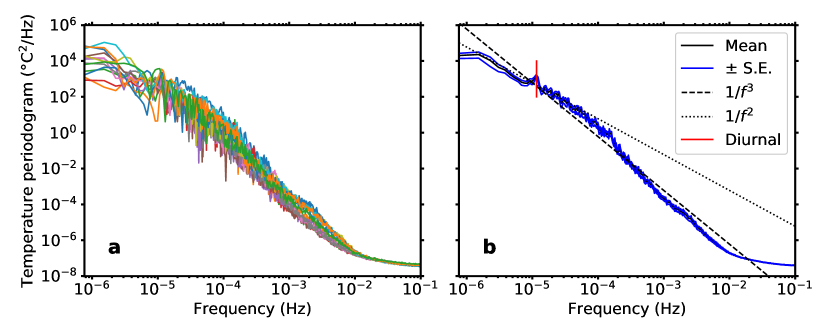
Figure 1: Temperature periodograms plotted on doubly-logarithmic coordinates. (a) Unaveraged periodograms $S_{\mathcal{T}}(f)$ versus frequency $f$, using the Thorlabs temperature detector. Though measured under different laboratory conditions, all 13 plots closely follow each other. (b) Averaged periodogram $\overline{S}_{\mathcal{T}}(f)$ versus frequency $f$. The solid black curve is the mean of all 13 periodograms displayed in (a). The two blue curves hugging the black curve represent standard-error values ($\pm$ S.E.). The averaged periodogram decreases approximately as $1/f^{2}$ (dotted curve) over the frequency range $1.0\times 10^{-6}\leq f<1.0\times 10^{-5}$ Hz and approximately as $1/f^{3}$ (dashed curve) over the range $1.0\times 10^{-5}\leq f\leq 2.5\times 10^{-2}$ Hz. The vertical red line segment marks a small hump at $1.16\times 10^{-5}$ Hz that corresponds to diurnal temperature variations (1 d = 86 400 s).

Indeed, the 13 curves presented in figure 1(a) are sufficiently similar that they may be averaged to improve the statistical accuracy of the data. To construct the averaged periodogram, a threshold of 198 048 measurements was determined to be the best compromise between including as many data sets, and as much of each, as possible. At 5 s per measurement, that corresponds to $L=990\,240$ s.

The next largest power of 2 greater than 198 048 is 262 144, or 1 310 720 s. The lowest observable frequency is very close to 1 $\mu$Hz; it could be reduced by zero-padding the data set. The highest observable frequency is the Nyquist limit $\frac{1}{2}/(5~{}\mathrm{s})=0.10$ Hz, as discussed in section 2.4. However, because of averaging of the values whose abscissas lie within a factor of 1.02, the highest displayed frequency is actually a bit smaller than 0.10 Hz, namely 0.098 Hz.

The outcome of the averaging process, displayed in figure 1(b), exhibits one log-unit of $1/f^{2}$ behavior (dotted curve) over the frequency range $1.0\times 10^{-6}\leq f<1.0\times 10^{-5}$ Hz, corresponding to $1.2<T_{f}\leq 11.6$ d; and several log-units of roughly $1/f^{3}$ behavior (dashed curve) that stretches from $1.0\times 10^{-5}$ to $2.5\times 10^{-2}$ Hz, corresponding to $40$ s $\leq T_{f}\leq 1.2$ d. The small hump in the curve at $1.16\times 10^{-5}$ Hz, designated by the vertical red line segment in the figure, corresponds to diurnal variations (1 d = 86 400 s). Since the periodogram displayed in figure 1b becomes essentially flat for $f\gtrsim 2.5\times 10^{-2}$ Hz, corresponding to $T_{f}\lesssim 40$ s, sampling the temperature at intervals shorter than $T_{s}=\frac{1}{2}T_{f}=20$ s does not provide additional information.

The observation of temperature fluctuations with a $1/f^{3}$ spectral signature is unexpected and surprising, and to our knowledge has not been reported previously.

3.2 Joint Temperature Measurements

We now proceed to demonstrate that the two independent temperature-measurement systems, the Thorlabs and ThermoWorks resistance temperature detectors discussed in section 2.2, yield similar results. The temperature periodograms displayed in figure 2(a) for both of these devices behave nearly indistinguishably for $f\lesssim 5\times 10^{-4}$ Hz, the frequency at which the baseline noise of the ThermoWorks detector becomes appreciable. The Thorlabs detector registers fluctuations over nearly two additional log-units of frequency, as is clear from figure 1(b).

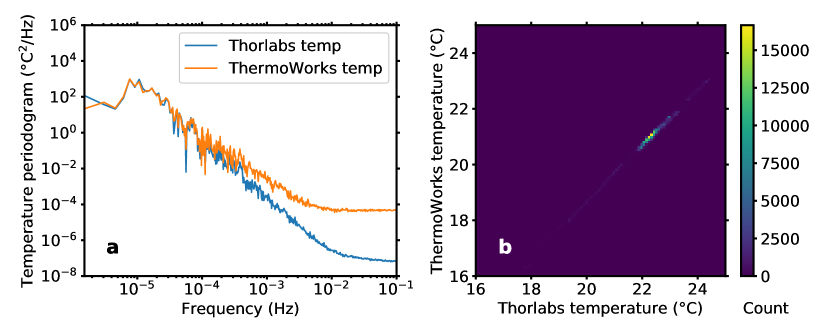
Figure 2: Measurements carried out with two independent temperature-measurement systems. The data presented in this figure were collected in an experiment of duration 7.51 d. (a) Temperature periodograms obtained with the Thorlabs and ThermoWorks temperature detectors, as indicated, plotted on doubly-logarithmic coordinates. The ThermoWorks device has higher baseline noise than the Thorlabs device. (b) Joint temperature measurements. The temperatures registered by the Thorlabs and ThermoWorks devices, plotted on the abscissa and ordinate, respectively, are highly correlated.

Joint temperature measurements for the two thermometric systems are displayed in figure 2(b). The overall mean temperatures $\overline{\mathcal{T}}$ and coefficients of variation CV registered by the temperature detectors were $\overline{\mathcal{T}}_{\mathrm{Thor}}=22.41^{\circ}$C and CV${}_{\mathrm{Thor}}=0.01262$ for the Thorlabs device, and $\overline{\mathcal{T}}_{\mathrm{Thermo}}=21.09^{\circ}$C and CV${}_{\mathrm{Thermo}}=0.01257$ for the ThermoWorks device. The measured overall mean temperatures differ by $1.32^{\circ}$C, which is within the margins of accuracy specified by the manufacturers: $\pm 3.0^{\circ}$C for the Thorlabs device and $\pm 0.5^{\circ}$C for the ThermoWorks device. The correlation coefficient for the temperature measurements is $\rho=0.9976$, verifying that our measurement methods are sound and that our results are consistent.

3.3 Ambient Temperature Scalograms

The ambient temperature scalograms portrayed in figure 3(a), plotted one atop the other, represent the 13 data sets whose periodograms are presented in figure 1(a). The choice of the Daubechies 4-tap wavelet variance for the scalogram is governed by a number of considerations, including the extended power-law exponent it accommodates and its insensitivity to constant values and linear trends [13, 14].

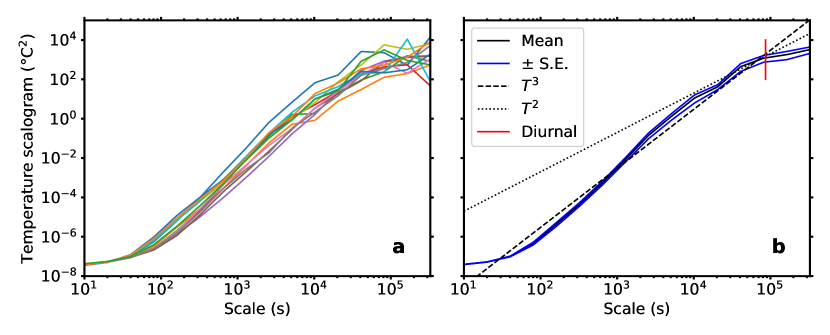
Figure 3: Temperature scalograms plotted on doubly-logarithmic coordinates. (a) Unaveraged Daubechies 4-tap wavelet variance $A_{\mathcal{T}}(T)$ versus scale $T$ using the Thorlabs temperature detector. As with the periodograms displayed in figure 1(a), all 13 plots closely follow each other even though they are measured under different laboratory conditions. (b) Averaged Daubechies 4-tap wavelet variance $\overline{A}_{\mathcal{T}}(T)$ versus scale $T$. The solid black curve is the mean of all 13 scalograms displayed in (a). The two blue curves hugging the black curve represent standard-error values ($\pm$ S.E.). The averaged scalogram increases approximately as $T^{3}$ (dashed curve) over the range $24\leq T\leq 6.7\times 10^{4}$ s, in correspondence with the $1/f^{3}$ decrease of the averaged periodogram portrayed in figure 1(b). The vertical red line segment depicts the scale for diurnal temperature variations (1 d = 86 400 s).

As with the periodograms, all of the scalograms in figure 3(a) follow each other sufficiently closely that they can be averaged to improve the statistical accuracy of the data. The outcome of the averaging process, displayed in figure 3(b), yields a result that grows roughly as $T^{3}$ over several log-units (dashed curve), stretching from $T=24$ s to $T=6.7\times 10^{4}$ s. The maximum permitted scale, corresponding to 1 sample, is 327 680 s or 3.8 d.

The observed power-law growth as $A(T)\propto T^{3}$ lies well below growth as $T^{5}$, where 5 is the maximum exponent permitted for the increase of the Daubechies 4-tap wavelet variance with scale and signals nonstationary behavior, as discussed in section 5.2.5 of Lowen & Teich [8]. The cubic form of the observed scalogram corresponds to the inverse-cubic form of the observed periodogram.

The averaged wavelet variance $\overline{A}_{\mathcal{T}}(T)$ displayed in figure 3(b) exhibits a small-scale cutoff at $T_{A}\approx 24$ s that separates behavior as $T^{0}$ from growth as $T^{3}$, and a large-scale cutoff at $T^{\prime}_{A}\approx 6.7\times 10^{4}$ s that separates growth as $T^{3}$ from growth as $T^{2}$. Similarly, the averaged periodogram $\overline{S}_{\mathcal{T}}(f)$ portrayed in figure 1(b) displays a low-frequency cutoff at $f^{\prime}_{S}\approx 1.0\times 10^{-5}$ Hz that separates decay as $1/f^{2}$ from decay as $1/f^{3}$, and a high-frequency cutoff at $f_{S}\approx 2.5\times 10^{-2}$ Hz that separates decay as $1/f^{3}$ from behavior as $1/f^{0}$. Thus, the low-frequency/large-scale cutoff product $f^{\prime}_{S}T^{\prime}_{A}\approx 0.67$ and the high-frequency/small-scale cutoff product $f_{S}T_{A}\approx 0.60$ are comparable, as expected.

The consistency of the scalograms and periodograms confirms that the computations for both measures are sound.

4 Conclusion and Discussion

We have presented a collection of periodograms that display the spectral characteristics of ambient temperature fluctuations collected in our laboratory under different conditions. A subset of those experiments made use of two independent temperature-measurement systems; the concurrence of the results confirms that our measurement methods are sound. Joint temperature measurements using data collected by both systems attest to the consistency of our results. A corresponding collection of scalograms comport with our periodograms, verifying that our computational methods are trustworthy. It is interesting to note that the issue of temperature fluctuations has a long history in the annals of physics, dating from the time of Gibbs [15], that has not been without controversy [16, 17, 18, 19].

We now proceed to demonstrate that our ambient temperature periodograms match those calculated from data collected at European weather stations over the frequency region where they overlap, providing support for the reliability of our experimental findings. In weather-station temperature analyses, it is customary to model measures such as periodogram in terms of decreasing piecewise power-law functions [20]; see, for example, Pelletier [21]. We show that the $1/f^{2}$ behavior observed in our periodograms accords with that observed at European weather stations over the same range of frequencies. This comparison is offered as an attestation to the validity of our experimental findings and not as commentary on a particular weather-analysis model.

In figure 4, we present temperature time-series periodograms collected at European weather stations in Hungary and Switzerland. The data in the lower curve, adapted from Jánosi, Vattay & Harnos [22], represent the unnormalized periodogram constructed from a temperature time series collected at the Hungarian Meteorological Service weather station in Szombathely (elevation 209 m), using a Hann window. Similar results were obtained for data collected at two other Hungarian weather stations, in Nyíregyháza (elevation 116 m) and in Győr (elevation 108 m).

The data in the upper curve, which are adapted from Talkner and Weber [23], represent the unnormalized periodogram constructed from a temperature time series comprising daily mean temperatures collected at the Schweizerische Meteorologische Anstalt weather station in Zürich (elevation 556 m), using a Welch window. A nearly identical periodogram was obtained from data collected at the Swiss Alpine weather station on Säntis mountain (elevation 2490 m). Temperature data collected at other low- and high-altitude Swiss weather stations also yielded similar periodograms.

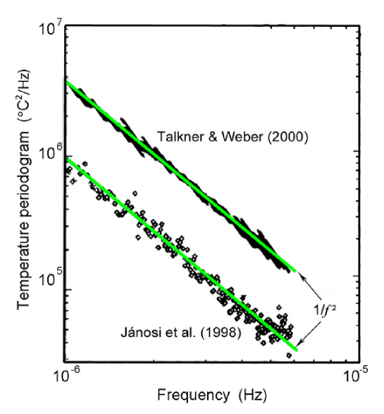
Figure 4: Temperature-time-series unnormalized periodograms collected at weather stations in Hungary and Switzerland, plotted on doubly-logarithmic coordinates. The straight lines, which are proportional to $1/f^{2}$, were chosen to best fit the data. The data are seen to behave as $1/f^{2}$ over the frequency range 0.1/d $\leq f<0.5/$d, corresponding to $2<T_{f}\leq 10$ d. In both studies, the maximum frequency reported in the periodogram is $\frac{1}{2}/$d $=5.79\times 10^{-6}$ Hz, corresponding to $T_{f}=2$ d, as mandated by the rate at which the underlying mean-temperature data were recorded, which was once daily ($T_{s}=1$ d). The data in the lower curve are adapted from Jánosi, Vattay & Harnos [22] while the data in the upper curve are adapted from Talkner and Weber [23].

The results of our laboratory measurements, presented in figure 1(b), are in accord with those presented in figure 4 over the spectral region that the three sets of data share. In particular, the periodograms of Jánosi, Vattay & Harnos [22] and Talkner and Weber [23] exhibit $1/f^{2}$ behavior over the range $2<T_{f}\leq 10$ d whereas our averaged indoor-temperature periodogram exhibits $1/f^{2}$ behavior over the range $1.2<T_{f}\leq 11.6$ d.

Spectral behavior of the form $1/f^{2}$ is often ascribed to temperature fluctuations that exhibit a random walk or ordinary Brownian motion. Although one might not expect that the spectral behavior of temperature time series collected in an indoor laboratory would coincide with those collected at a European weather station, the explanation for this conjunction may lie in the work of Jánosi, Vattay & Harnos [22]. These authors have compared the spectral properties of temperature measurements conducted in small laboratory convection cells [24] with those of extensive meteorological weather stations. The statistical character of the temperature fluctuations in small-scale laboratory experiments may resemble that exhibited by the diurnal atmospheric boundary layer by virtue of the hydrodynamical similarity between these seemingly different systems.

In any case, our temperature periodograms extend to substantially higher frequencies than those of Jánosi, Vattay & Harnos [22] and Talkner and Weber [23] because of the far higher rate at which we sampled the temperature, namely every 5 s. And it is at these higher frequencies, in particular over the frequency range $1.0\times 10^{-5}\leq f\leq 2.5\times 10^{-2}$ Hz, corresponding to 40 s $\leq T_{f}\leq 1.2$ d, that we observe $1/f^{3}$ spectral behavior. We have shown that the periodograms and scalograms in our ambient temperature measurements clearly follow such cubic-law behavior; formulating a rationale with respect to why this is so is a work in progress.

ORCID iDs

Steven B. Lowen https://orcid.org/0000-0002-5243-2548
Malvin Carl Teich https://orcid.org/0000-0001-8164-4622

References

References

- [1] A. L. Hodgkin and B. Katz. The effect of temperature on the electrical activity of the giant axon of the squid. Journal of Physiology (London), 109:240–249, 1949.
- [2] J. O. Josefsberg and B. Buckland. Vaccine process technology. Biotechnology and Bioengineering, 109(6):1443–1460, 2012.
- [3] B. E. A. Saleh and M. C. Teich. Fundamentals of Photonics. Wiley, Hoboken, 3rd edition, 2019.
- [4] B. P. Abbott et al. Observation of gravitational waves from a binary black hole merger. Physical Review Letters, 116:061102, 2016.
- [5] N. Mohan, S. B. Lowen, and M. C. Teich. Photon-count fluctuations exhibit inverse-square baseband spectral behavior that extends to Hz. Physical Review Research, 2:013170, 2020.
- [6] N. Mohan. Photon-Counting Optical Coherence-Domain Imaging. PhD thesis, Boston University, Boston, MA, 2010.
- [7] A. V. Oppenheim and R. W. Schafer. Discrete-Time Signal Processing. Pearson, New York, 3rd edition, 2009.
- [8] S. B. Lowen and M. C. Teich. Fractal-Based Point Processes. Wiley, Hoboken, 2005.
- [9] I. Daubechies. Ten Lectures on Wavelets. Society for Industrial and Applied Mathematics, Philadelphia, 1992.
- [10] A. Haar. Zur Theorie der orthogonalen Funktionensysteme. Mathematische Annalen, 69:331–371, 1910.
- [11] A. Graps. An introduction to wavelets. IEEE Computational Science and Engineering, 2(2):50–61, 1995.
- [12] Ø. Ryan. Linear Algebra, Signal Processing, and Wavelets–A Unified Approach. Springer Nature, Cham, Switzerland, 2019.
- [13] M. Vetterli and J. Kovačević. Wavelets and Subband Coding. Prentice–Hall, New York, 1995.
- [14] M. C. Teich, C. Heneghan, S. M. Khanna, Å. Flock, M. Ulfendahl, and L. Brundin. Investigating routes to chaos in the guinea-pig cochlea using the continuous wavelet transform and the short-time Fourier transform. Annals of Biomedical Engineering, 23:583–607, 1995.
- [15] J. W. Gibbs. The Collected Works of J. Willard Gibbs, volume 2. Yale University Press, New Haven, 1948.
- [16] L. D. Landau, E. M. Lifshitz, and L. P. Pitaevskii. Statistical Physics: Part I. In Course in Theoretical Physics, volume 5, chapter 7. Butterworth-Heinemann/Elsevier, Oxford, 3rd edition, 1980.
- [17] C. Kittel. Temperature fluctuation: An oxymoron. Physics Today, 41(5):93, 1988.
- [18] B. B. Mandelbrot. Temperature fluctuation: A well-defined and unavoidable notion. Physics Today, 42(1):71–73, 1989.
- [19] T. C. P. Chui, D. R. Swanson, M. J. Adriaans, J. A. Nissen, and J. A. Lipa. Temperature fluctuations in the canonical ensemble. Physical Review Letters, 69:3005–3008, 1992.
- [20] I. Eliazar. Power Laws: A Statistical Trek. Springer Nature, Cham, Switzerland, 2020.
- [21] J. D. Pelletier. Analysis and modeling of the natural variability of climate. Journal of Climate, 10:1331–1342, 1997.
- [22] I. M. Jánosi, G. Vattay, and A. Harnos. Turbulent helium gas cell as a new paradigm of daily meteorological fluctuations? Journal of Statistical Physics, 93:919–926, 1998.
- [23] P. Talkner and R. O. Weber. Power spectrum and detrended fluctuation analysis: Application to daily temperatures. Physical Review E, 62:150–160, 2000.
- [24] X.-Z. Wu, L. Kadanoff, A. Libchaber, and M. Sano. Frequency power spectrum of temperature fluctuations in free convection. Physical Review Letters, 64:2140–2143, 1990.