A unified view of
likelihood ratio and reparameterization gradients
and an optimal importance sampling scheme

Abstract

Reparameterization (RP) and likelihood ratio (LR) gradient estimators are used throughout machine and reinforcement learning; however, they are usually explained as simple mathematical tricks without providing any insight into their nature. We use a first principles approach to explain LR and RP, and show a connection between the two via the divergence theorem. The theory motivated us to derive optimal importance sampling schemes to reduce LR gradient variance. Our newly derived distributions have analytic probability densities and can be directly sampled from. The improvement for Gaussian target distributions was modest, but for other distributions such as a Beta distribution, our method could lead to arbitrarily large improvements, and was crucial to obtain competitive performance in evolution strategies experiments.

 

A unified view of likelihood ratio and reparameterization gradients
and an optimal importance sampling scheme

 

Paavo Parmas^∗                        Masashi Sugiyama

Okinawa Institute of Science and Technology paavo.parmas@oist.jp                        RIKEN and The University of Tokyo sugi@k.u-tokyo.ac.jp

1 Introduction

Both likelihood ratio (LR) gradients (Glynn,, 1990; Williams,, 1992) and reparameterization (RP) gradients (Rezende et al.,, 2014; Kingma and Welling,, 2013) can be used to obtain unbiased estimates of the gradient of an expectation w.r.t. the parameters of the distribution: $\frac{\textup{d}\hfill}{\textup{d}\theta\hfill}\mathbb{E}_{x\sim p\left(x;\theta\right)}\left[\phi(x)\right]$. This problem is fundamental in machine learning (Mohamed et al.,, 2019), and the gradients are used for optimization in a wide range of tasks (Schulman et al., 2015a, ; Weber et al.,, 2019; Parmas,, 2018), e.g. reinforcement learning (Sutton and Barto,, 1998; Schulman et al., 2015b, ; Schulman et al.,, 2017; Sutton et al.,, 2000; Peters and Schaal,, 2008), stochastic variational inference (Hoffman et al.,, 2013) and evolutionary algorithms (Wierstra et al.,, 2008; Salimans et al.,, 2017; Ha and Schmidhuber,, 2018; Conti et al.,, 2018).

The LR gradient is usually derived as $\frac{\textup{d}\hfill}{\textup{d}\theta\hfill}\mathbb{E}_{x\sim p\left(x;\theta\right)}\left[\phi(x)\right]=\int\frac{\textup{d}p\left(x;\theta\right)\hfill}{\textup{d}\theta\hfill}\phi(x)\textup{d}x=\int p\left(x;\theta\right)\frac{\frac{\textup{d}p\left(x;\theta\right)\hfill}{\textup{d}\theta\hfill}}{p\left(x;\theta\right)}\phi(x)\textup{d}x=\int p\left(x;\theta\right)\frac{\textup{d}\log p\left(x;\theta\right)\hfill}{\textup{d}\theta\hfill}\phi(x)\textup{d}x=\mathbb{E}_{x\sim p\left(x;\theta\right)}\left[\frac{\textup{d}\log p\left(x;\theta\right)\hfill}{\textup{d}\theta\hfill}\phi(x)\right]$. On the other hand, the RP gradient is derived by defining a mapping $g(\epsilon)=x$, where $\epsilon$ is sampled from a fixed simple distribution, but $x$ ends up being sampled from the desired distribution. For example, if $x$ is Gaussian $x\sim\mathcal{N}(\mu,\sigma)$, then the required mapping is $g(\epsilon)=\mu+\sigma\epsilon$, where $\epsilon\sim\mathcal{N}(0,1)$, and the RP gradient is derived as $\frac{\textup{d}\hfill}{\textup{d}\theta\hfill}\mathbb{E}_{x\sim p\left(x;\theta\right)}\left[\phi(x)\right]=\frac{\textup{d}\hfill}{\textup{d}\theta\hfill}\mathbb{E}_{\epsilon\sim\mathcal{N}(0,1)}\left[\phi\left(g(\epsilon)\right)\right]=\mathbb{E}_{\epsilon\sim\mathcal{N}(0,1)}\left[\frac{\textup{d}\phi\left(g(\epsilon)\right)\hfill}{\textup{d}\theta\hfill}\right]=\mathbb{E}_{\epsilon\sim\mathcal{N}(0,1)}\left[\frac{\textup{d}g\hfill}{\textup{d}\theta\hfill}\frac{\textup{d}\phi\left(g(\epsilon)\right)\hfill}{\textup{d}g\hfill}\right]$, where $\theta=[\mu,\sigma]$, $\frac{\textup{d}g\hfill}{\textup{d}\mu\hfill}=1$, $\frac{\textup{d}g\hfill}{\textup{d}\sigma\hfill}=\epsilon$ and $\frac{\textup{d}\phi\left(g(\epsilon)\right)\hfill}{\textup{d}g\hfill}=\frac{\textup{d}\phi\left(x\right)\hfill}{\textup{d}x\hfill}$.

What do these derivations mean, and what is the relationship between the methods? We give two possible answers to this question in Secs. 2 and 3, then explain that the LR gradient is the unique unbiased estimator that weights the function values $\phi(x)$, and motivate importance sampling from a different distribution $q(x)$ to reduce LR gradient variance. Our optimal importance sampling scheme is reminiscent of the optimal reward baseline for reducing LR gradient variance (Weaver and Tao,, 2001) (App. A), but our result is orthogonal, and can be combined with such prior methods.

Further background and related work:

The variance of LR and RP gradients has been of central importance in their research. Typically, RP is said to be more accurate and scale better with the sampling dimension (Rezende et al.,, 2014)—this claim is also backed by theory (Xu et al.,, 2019; Nesterov and Spokoiny,, 2017); however, there is no guarantee that RP outperforms LR. In particular, for multimodal $\phi(x)$ (Gal,, 2016) or chaotic systems (Parmas et al.,, 2018), LR can be arbitrarily better than RP (e.g., the latter showed that LR can be $10^{6}$ more accurate in practice). Moreover, RP is not directly applicable to discrete sampling spaces, but requires continuous relaxations (Maddison et al.,, 2016; Jang et al.,, 2016; Tucker et al.,, 2017). Differentiable RP is also not always possible, but implicit RP gradients have increased the number of usable distributions (Figurnov et al.,, 2018). Techniques for variance reduction have been extensively studied, including control variates/baselines (Greensmith et al.,, 2004; Grathwohl et al.,, 2017; Tucker et al.,, 2018; Gu et al.,, 2015; Geffner and Domke,, 2018; Gu et al.,, 2016) as well as Rao-Blackwellization (Titsias and Lázaro-Gredilla,, 2015; Ciosek and Whiteson,, 2018; Asadi et al.,, 2017). One can also combine the best of both LR and RP gradients by dynamically reweighting them (Parmas et al.,, 2018; Metz et al.,, 2019). Importance sampling for reducing LR gradient variance was previously considered in variational inference (Ruiz et al.,, 2016), but they proposed to sample from the same distribution while tuning the variance, whereas in our work we derive an optimal distribution. In reinforcement learning, importance sampling has been studied for sample reuse via off-policy policy evaluation (Thomas and Brunskill,, 2016; Jiang and Li,, 2016; Gu et al.,, 2017; Munos et al.,, 2016; Jie and Abbeel,, 2010), but modifying the policy to improve gradient accuracy has not been considered. The flow theory in Sec. 3 was concurrently derived by Jankowiak and Obermeyer, (2018), but their work focused on deriving new RP gradient estimators, and they do not discuss the duality. Our derivation is also more visual.

2 A probability “boxes” view of LR and RP gradients

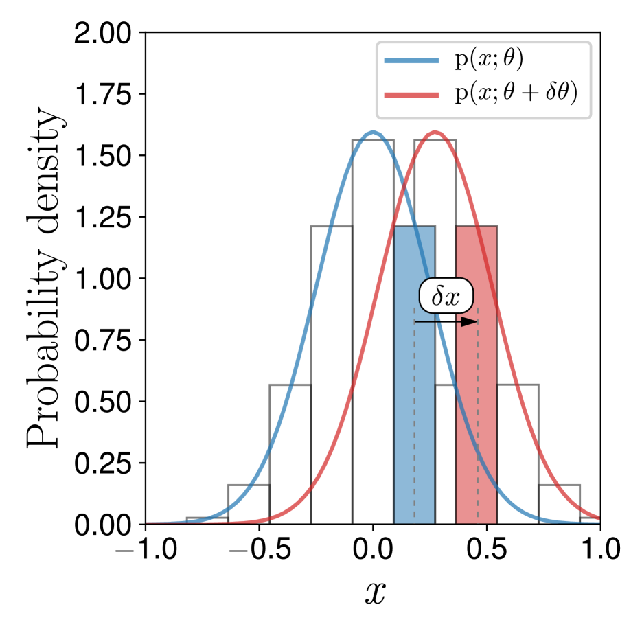
(a) RP probability “boxes”

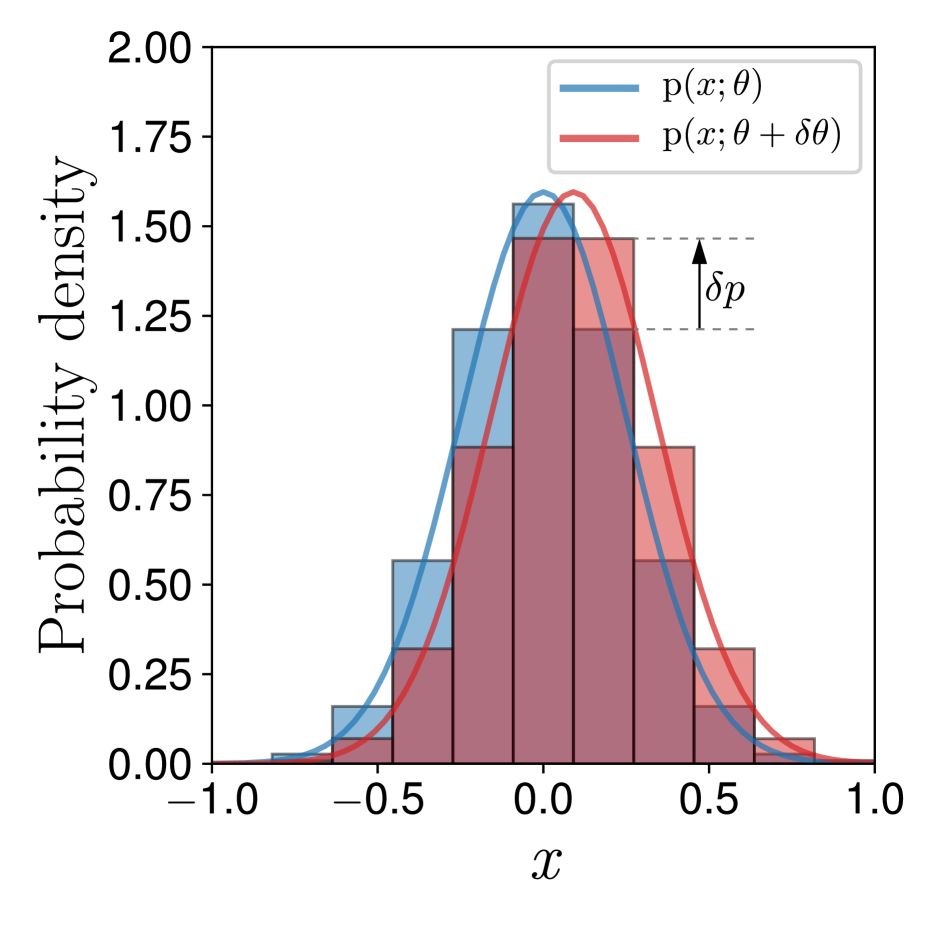
(b) LR probability “boxes”

Figure 1: LR keeps the boundaries of the “boxes” fixed, while RP keeps the probability mass fixed.

Here we give the first of our two explanations of the link between LR and RP gradients. The explanation relies on a first principles thinking about the effect that changing the parameters of a probability distribution $\theta$ has on infinitesimal “boxes” of probability mass (Fig. 1). Both LR and RP are trying to estimate $\frac{\textup{d}\hfill}{\textup{d}\theta\hfill}\int p\left(x;\theta\right)\phi(x)\textup{d}x$. A typical finite explanation of Riemann integrals is performed by discretizing the integrand into “boxes” of size $\Delta x$, and summing: $\frac{\textup{d}\hfill}{\textup{d}\theta\hfill}\sum_{i=1}^{N}p\left(x_{i};\theta\right)\Delta x_{i}\phi(x_{i})$. Taking the limit as $N\rightarrow\infty$ recovers the true integral. In this equation $p\left(x_{i};\theta\right)\Delta x_{i}$ is the amount of probability mass inside the “box”, and $\phi(x_{i})$ is the function value inside the “box”.

Such a view can be used to explain RP gradients. In this case, the boundaries of the “box” are fixed with reference to the shape of the probability distribution, i.e. for each $i$ we define the center of the box as $x_{i}=g(\epsilon_{i};\theta)$, and the boundaries as $g(\epsilon_{i}\pm\Delta\epsilon/2;\theta)$, where $\epsilon_{i}$ is the reference position on a fixed simple distribution $p\left(\epsilon\right)$. the amount of probability mass assigned to each “box” stays fixed at $\Delta p_{i}=p\left(\epsilon\right)\Delta\epsilon~{};$ however, the center of the “box” moves, so the function value $\phi(x_{i})$ inside each “box” changes by $\delta\phi_{i}=\phi\left(g(\epsilon_{i};\theta+\delta\theta)\right)-\phi\left(g(\epsilon_{i};\theta)\right)=\phi(x_{i}+\delta x_{i})-\phi(x_{i})$. The full derivative can then be expressed as $\frac{\textup{d}\hfill}{\textup{d}\theta\hfill}\mathbb{E}_{x\sim p\left(x;\theta\right)}\left[\phi(x)\right]\approx\frac{1}{\delta\theta}\sum_{i=1}^{N}\Delta p_{i}\delta\phi_{i}=\sum_{i=1}^{N}\Delta p_{i}\frac{\delta\phi_{i}}{\delta x_{i}}\frac{\delta x_{i}}{\delta\theta}$. Taking the infinitesimal limit as $N\rightarrow\infty$, and noting $\Delta p_{i}=p\left(x_{i};\theta\right)\Delta x_{i}$, we obtain the RP gradient estimator $\int p\left(x;\theta\right)\frac{\textup{d}\phi(x)\hfill}{\textup{d}x\hfill}\frac{\textup{d}x\hfill}{\textup{d}\theta\hfill}~{}\textup{d}x$. We see that RP essentially estimates the gradient by keeping the probability mass inside each “box” fixed, but estimating how the function value $\phi$ inside the “box” changes as the parameters $\theta$ are perturbed.

The LR gradient, on the other hand, keeps the boundaries of the “boxes” fixed, i.e. the centre of the box is at $x_{i}$, and the boundaries at $x_{i}\pm\Delta x_{i}/2$. Now, as the boundaries are independent of $\theta$, the function value $\phi(x_{i})$ inside the box stays fixed, even as $\theta$ is perturbed by $\delta\theta$; however, the probability mass inside the box changes, because the density changes by $\delta p_{i}=p\left(x_{i};\theta+\delta\theta\right)-p\left(x_{i};\theta\right)$. The full derivative can be expressed as $\frac{\textup{d}\hfill}{\textup{d}\theta\hfill}\mathbb{E}_{x\sim p\left(x;\theta\right)}\left[\phi(x)\right]\approx\frac{1}{\delta\theta}\sum_{i=1}^{N}\Delta x_{i}\delta p_{i}\phi(x_{i})=\sum_{i=1}^{N}p\left(x_{i};\theta\right)\Delta x_{i}\frac{\delta p_{i}/\delta\theta}{p\left(x_{i};\theta\right)}\phi(x_{i})$. Where we have multiplied and divided by $p\left(x_{i};\theta\right)$. Taking the infinitesimal limit recovers the LR gradient $\int p\left(x;\theta\right)\frac{\frac{\textup{d}p\left(x;\theta\right)\hfill}{\textup{d}\theta\hfill}}{p\left(x;\theta\right)}\phi(x)~{}\textup{d}x=\mathbb{E}_{x\sim p\left(x;\theta\right)}\left[\frac{\frac{\textup{d}p\left(x;\theta\right)\hfill}{\textup{d}\theta\hfill}}{p\left(x;\theta\right)}\phi(x)\right]$. The transformation $p\left(x;\theta\right)\frac{\frac{\textup{d}p\left(x;\theta\right)\hfill}{\textup{d}\theta\hfill}}{p\left(x;\theta\right)}=p\left(x;\theta\right)\frac{\textup{d}\log p\left(x;\theta\right)\hfill}{\textup{d}\theta\hfill}$ is known as the log-derivative trick, and it may appear to be the essence behind the LR gradient, but actually the multiplication and division by $p(x;\theta)$ is just a special case of the more general Monte Carlo integration principle. Any integral $\int f(x)~{}\textup{d}x$ can be approximated by sampling from a distribution $q(x)$ as $\int f(x)~{}\textup{d}x=\int q(x)\frac{f(x)}{q(x)}~{}\textup{d}x=\mathbb{E}_{x\sim q(x)}\left[\frac{f(x)}{q(x)}\right]$. Rather than thinking of the LR gradient in terms of the log-derivative term, it may be better to think of it as simply estimating the integral $\int\frac{\textup{d}p\left(x;\theta\right)\hfill}{\textup{d}\theta\hfill}\phi(x)~{}\textup{d}x$ by applying the appropriate importance weights to samples from $p(x;\theta)$. Thus, we see that in the discretized case, the LR gradient picks $q(x)=p\left(x;\theta\right)$ (Jie and Abbeel,, 2010) and performs Monte Carlo integration to approximate $\frac{1}{\delta\theta}\sum_{i=1}^{N}\Delta x_{i}\delta p_{i}\phi(x_{i})$ by sampling from $P(x_{i})=\Delta x_{i}p\left(x_{i};\theta\right)$. To summarize: LR estimates the gradient by keeping the boundaries of the boxes fixed, measuring the change in probability mass in each box, and weighting by the function value: $\phi(x_{i})\delta p$.

Sometimes, the LR gradient is described as being “kind of like a finite difference gradient” (Salimans et al.,, 2017; Mania et al.,, 2018), but here we see that it is a different concept, which does not rely on fitting a straight line between differences of $\phi$ (App. A), but estimates how probability mass is reallocated among different $\phi$ values via Monte Carlo integration by sampling from $p\left(x;\theta\right)$.

3 A unified probability flow view of LR and RP gradients

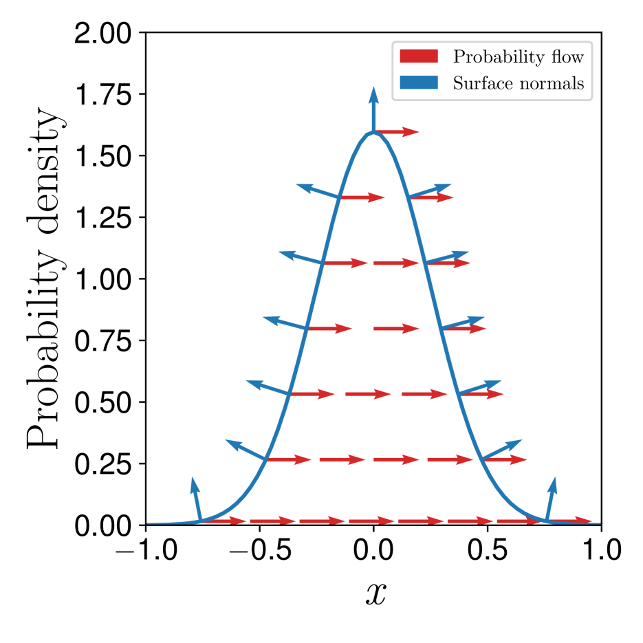
(a) $\mu$ flow lines

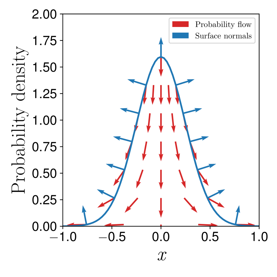
(b) $\sigma$ flow lines

Figure 2: Probability flow lines when $\mu$ and $\sigma$ are perturbed.

Here we give another explanation of LR and RP. The appeal of this theory is that both LR and RP come out of the same derivation, thus showing a link between the two. In particular, we define a virtual incompressible flow of probability mass imposed by perturbing the parameters $\theta$ of $p\left(x;\theta\right)$, which can be used to express the derivative of the expectation as an integral over this flow. LR and RP estimators correspond to duals of this integral under the divergence theorem (App. B).

The main idea resembles RP, but in addition to sampling the ${\bf x}$ location, we sample a height $h$ for each point: $h=\epsilon_{h}p\left({\bf x};\theta\right)$, where $\epsilon_{h}\sim\textup{unif}(0,1)$, i.e., the sampling space is extended with an additional dimension for the height $\tilde{{\bf x}}=[{\bf x}^{T},h]^{T}$, and we are uniformly sampling in the volume under $p\left({\bf x};\theta\right)$. The definition of $g$ in the introduction is extended, s.t. $\tilde{g}(\epsilon_{x},\epsilon_{h})=\tilde{{\bf x}}$. The expectation turns into:

$$\frac{\textup{d}\hfill}{\textup{d}\theta\hfill}\int p\left({\bf x};\theta\right)\phi({\bf x})\textup{d}{\bf x}$$ (1)

$$=\frac{\textup{d}\hfill}{\textup{d}\theta\hfill}\int_{\epsilon_{x}}\int_{\epsilon_{h}}p\left(\epsilon_{x}\right)p\left(\epsilon_{h}\right)\phi\left(\tilde{g}(\epsilon_{x},\epsilon_{h})\right)\textup{d}\epsilon_{x}\textup{d}\epsilon_{h}$$

$$=\int_{V}\nabla_{\tilde{{\bf x}}}\phi(\tilde{{\bf x}})\nabla_{\theta}\tilde{g}(\epsilon_{x},\epsilon_{h})\textup{d}V.$$

In Eq. (1), $V$ is the volume under the curve, and $\phi([{\bf x}^{T},h]^{T})\coloneqq\phi({\bf x})$ ignores the $h$-component. Each column $i$ of $\nabla_{\theta}\tilde{g}(\epsilon_{x},\epsilon_{h})$ corresponds to a vector field induced by perturbing the $i^{\textup{th}}$ component of $\theta$. The red lines in Fig. 2 show the induced flow fields for a Gaussian distribution as the mean and variance are perturbed. The other member of the integral, $\nabla_{\tilde{{\bf x}}}\phi(\tilde{{\bf x}})$ is the grad of the scalar field $\phi(\tilde{{\bf x}})$. As $\phi$ does not depend on $h$, the grad will always be parallel to the ${\bf x}$ axes with magnitude $\frac{\textup{d}\phi\hfill}{\textup{d}{\bf x}\hfill}$.

According to the divergence theorem, the volume integral in Eq. (1) can be turned into a surface integral over the boundary ${\bf S}$ ($\textup{d}{\bf S}$ is a shorthand for $\hat{{\bf n}}\textup{d}S$, where $\hat{{\bf n}}$ is the surface normal vector):

$$\int_{V}\nabla\cdot{\bf F}\textup{d}V=\int_{S}{\bf F}\textup{d}{\bf S}.$$ (2)

In Eq. (2), ${\bf F}$ is any vector field. A common corollary arises by picking ${\bf F}=\phi{\bf v}$, where $\phi$ is a scalar field, and ${\bf v}$ is a vector field. We choose ${\bf v}=\nabla_{\theta}\tilde{g}(\epsilon_{x},\epsilon_{h})\delta\theta$, where $\delta\theta$ is an arbitrary perturbation in $\theta$, so that ${\bf F}=\phi(\tilde{{\bf x}})\nabla_{\theta}\tilde{g}(\epsilon_{x},\epsilon_{h})\delta\theta$, in which case $\nabla\cdot{\bf F}=\nabla\cdot\left(\phi(\tilde{{\bf x}})\nabla_{\theta}\tilde{g}(\epsilon_{x},\epsilon_{h})\delta\theta\right)=\nabla_{\tilde{{\bf x}}}\phi(\tilde{{\bf x}})\nabla_{\theta}\tilde{g}(\epsilon_{x},\epsilon_{h})\delta\theta+\phi(\tilde{{\bf x}})\nabla_{\tilde{{\bf x}}}\cdot\nabla_{\theta}\tilde{g}(\epsilon_{x},\epsilon_{h})\delta\theta$. Note that the term $\nabla_{\theta}\tilde{g}(\epsilon_{x},\epsilon_{h})\delta\theta$ corresponds to an incompressible flow (because the probability density does not change at any point in the augmented space). As the div of an incompressible flow is 0, then $\nabla_{\tilde{{\bf x}}}\cdot\nabla_{\theta}\tilde{g}(\epsilon_{x},\epsilon_{h})\delta\theta=0$, and the second term disappears. Noting that $\delta\theta$ can be canceled, because it is arbitrary, we are left with the equation:

$$\int_{V}\nabla_{\tilde{{\bf x}}}\phi(\tilde{{\bf x}})\nabla_{\theta}\tilde{g}(\epsilon_{x},\epsilon_{h})\textup{d}V =\int_{S}\phi(\tilde{{\bf x}})\nabla_{\theta}\tilde{g}(\epsilon_{x},\epsilon_{h})\textup{d}{\bf S}.$$ (3)

Now we explain how the left-hand side of Eq. (3) gives rise to the RP gradient estimator, while the right-hand side corresponds to the LR gradient estimator.

RP estimator:

Consider the $\nabla_{\tilde{{\bf x}}}\phi(\tilde{{\bf x}})\nabla_{\theta}\tilde{g}(\epsilon_{x},\epsilon_{h})$ term. As the scalar field $\phi(\tilde{{\bf x}})$ is independent of the height location $h$, the component of the grad in that direction is 0, and $\phi(\tilde{{\bf x}})=\phi({\bf x})$. As the $h$-component is 0, then the value of $\tilde{g}$ in the $h$-direction is multiplied by 0, and is irrelevant for the product, so $\nabla_{\tilde{{\bf x}}}\phi(\tilde{{\bf x}})\nabla_{\theta}\tilde{g}(\epsilon_{x},\epsilon_{h})=\nabla_{{\bf x}}\phi({\bf x})\nabla_{\theta}g(\epsilon_{x})$, which is just the term used in the RP estimator. Hence, the left-hand side of Eq. (3) corresponds to the RP gradient.

LR estimator:

We will show that the LR estimator tries to integrate $\int_{S}\phi(\tilde{{\bf x}})\nabla_{\theta}\tilde{g}(\epsilon_{x},\epsilon_{h})\textup{d}{\bf S}$. To do so, note that $\textup{d}{\bf S}=\hat{{\bf n}}\textup{d}S$. It is necessary to express the normalized surface vector $\hat{{\bf n}}$, and then perform the integral over the surface. The derivation is in App. B.2, and the final result is:

$$\int_{S}\phi(\tilde{{\bf x}})\nabla_{\theta}\tilde{g}(\epsilon_{x},\epsilon_{h})~{}\textup{d}{\bf S}=\int_{X}\phi({\bf x})\frac{\textup{d}p\left({\bf x};\theta\right)\hfill}{\textup{d}\theta\hfill}~{}\textup{d}{\bf x}.$$ (4)

We have already seen that a Monte Carlo integration of the right-hand side of Eq. (4) using samples from $p\left({\bf x};\theta\right)$ yields the LR gradient estimator. Thus, the RP and LR are duals under the divergence theorem. To further strengthen this claim we prove that the LR gradient estimator is the unique estimator that takes weighted averages of the function values $\phi({\bf x})$.

Theorem 1 (Uniqueness of LR estimator)

$\psi({\bf x})=p\left({\bf x};\theta\right)\frac{\textup{d}\log p\left({\bf x};\theta\right)\hfill}{\textup{d}\theta\hfill}$ is the unique function $\psi({\bf x})$, s.t. $\int\psi({\bf x})\phi({\bf x})\textup{d}{\bf x}=\frac{\textup{d}\hfill}{\textup{d}\theta\hfill}\int p\left({\bf x};\theta\right)\phi({\bf x})\textup{d}{\bf x}$ for any $\phi({\bf x})$.

Proof. Suppose that there exist $\psi({\bf x})$ and $f({\bf x})$, s.t. $\int\phi({\bf x})\psi({\bf x})~{}\textup{d}{\bf x}=\int\phi({\bf x})f({\bf x})~{}\textup{d}{\bf x}$ for any $\phi({\bf x})$. Rearrange the equation into $\int\phi({\bf x})\left(\psi({\bf x})-f({\bf x})\right)~{}\textup{d}{\bf x}=0$, then pick $\phi({\bf x})=\psi({\bf x})-f({\bf x})$ from which we get $\int\left(\psi({\bf x})-f({\bf x})\right)^{2}~{}\textup{d}{\bf x}=0$. Therefore, $\psi=f$. Q.E.D.

We see that Eq. (4) was immediately clear without having to go through the derivation. The same analysis does not work for RP (App. C). Indeed, there are infinitely many RP gradients (Jankowiak and Obermeyer,, 2018). Moreover, the analysis does not consider coupled sampling of ${\bf x}$ (Walder et al.,, 2019).

4 Slice ratio importance sampling

As LR is the only unbiased gradient estimator that weights samples of $\phi(x)$ (Sec. 3), what could be done to reduce its variance? One underexplored option is to keep the product $p\left({\bf x};\theta\right)\frac{\textup{d}\log p\left({\bf x};\theta\right)\hfill}{\textup{d}\theta\hfill}$ the same, but sample from a different distribution $q(x)$ using importance sampling $q(x)p\left({\bf x};\theta\right)\frac{\textup{d}\log p\left({\bf x};\theta\right)\hfill}{\textup{d}\theta\hfill}\nicefrac{{1}}{{q(x)}}$. How to pick $q(x)$? Our first attempt (App. D, Fig. 3(b)) was suboptimal.

Optimal importance sampling for minimum gradient variance:

We seek a distribution $q(x)$, s.t. the variance of $\frac{\textup{d}p\left(x;\theta\right)\hfill}{\textup{d}\theta\hfill}\phi(x)/q(x)$ is minimized. The derivation is analogous to the standard result for optimal importance sampling in statistics (Owen,, 2013). As $\phi(x)$ is not known a priori, we minimize the variance of $\frac{\textup{d}p\left(x;\theta\right)\hfill}{\textup{d}\theta\hfill}/q(x)$. The omission is well-justified in the multidimensional setting, as most of the variation in $\phi({\bf x})$ is caused by the other dimensions and can thus be viewed as noise. See also App. F.2 for several other justifications. The variance can be expressed as $\int q(x)\left(\frac{\frac{\textup{d}p\left(x;\theta\right)\hfill}{\textup{d}\theta\hfill}}{q(x)}\right)^{2}~{}\textup{d}x$. Adding in the constraint $\int q(x)~{}\textup{d}x=1$ with a Lagrange multiplier $\lambda$, and performing a variational optimization by setting the derivative w.r.t. $q$ to 0 we have:

$$-\left(\frac{\frac{\textup{d}p\left(x;\theta\right)\hfill}{\textup{d}\theta\hfill}}{q(x)}\right)^{2}+\lambda=0~{}~{}\Rightarrow~{}~{}q(x)=\left|\frac{\textup{d}p\left(x;\theta\right)\hfill}{\textup{d}\theta\hfill}\right|/\sqrt{\lambda}~{}.$$ (5)

Eq. (5) tells that the optimal importance sampling distribution is proportional to the magnitude of the gradient of the base distribution. How to normalize this distribution, and how to sample from it?

For a Gaussian distribution, we can derive two possible distributions: one for $\mu$ (Fig. 3(c)) and one for $\sigma$ (Fig. 3(d)). The derivative w.r.t $\mu$ appears more important, so we derive it first. Note that $\frac{\textup{d}p\left(x\right)\hfill}{\textup{d}\mu\hfill}=-\frac{\textup{d}p\left(x\right)\hfill}{\textup{d}x\hfill}$, and that by sampling a height $h$ and transforming from the $h$-coordinate to the $x$-coordinate via $x=p^{-1}(h)$, the probability density is weighted: $\textup{d}h=\left|\frac{\textup{d}p\left(x\right)\hfill}{\textup{d}x\hfill}\right|\textup{d}x$ (App. D). This insight allows us to derive the distribution and a sampling method (App. E.2). Namely, to sample from the distribution: 1) sample $h\sim\textup{unif}(0,p_{\mathrm{max}})$, where $p_{\mathrm{max}}=p\left(\mu;\mu,\sigma\right)$ is the peak probability density, 2) compute the location of the edge of the slice $x=p^{-1}(h)$ (Fig. 3(a)). Putting these results together, one obtains the pdf, a sampling method and the LR gradient estimator:

$$p_{B}\left(x;\mu,\sigma\right)=\frac{|x-\mu|}{2\sigma^{2}}\exp\left(\frac{-(x-\mu)^{2}}{2\sigma^{2}}\right),$$ (6)

$$x=\mu\pm\sigma\sqrt{-2\log(\epsilon_{h})}~{}~{}~{}\textup{where}~{}~{}~{}\epsilon_{h}\sim\textup{unif}(0,1),$$

$$\frac{\textup{d}\hfill}{\textup{d}\mu\hfill}\mathbb{E}_{x\sim p\left(x\right)}\left[\phi(x)\right]=\mathbb{E}_{x\sim q(x)}\left[\textup{sgn}(x-\mu)\frac{2}{\sigma\sqrt{2\pi}}\phi(x)\right].$$

We call the derived distribution the B-distribution (Fig. 3(c)), and the resulting gradient estimator the slice ratio gradient (SLRG). Notice that the B-distribution is the Rayleigh distribution symmetrized about the origin. The derivation for $\sigma$ is similar (App. E.4), but note, $\frac{\textup{d}p\left(x\right)\hfill}{\textup{d}\sigma\hfill}=\sigma\frac{\textup{d}^{2}p\left(x\right)\hfill}{\textup{d}x^{2}\hfill}$ for a Gaussian.

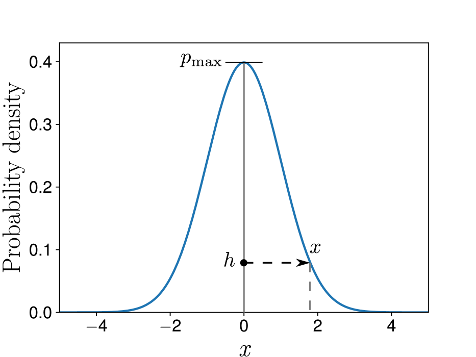
(a) Slice ratio sampling

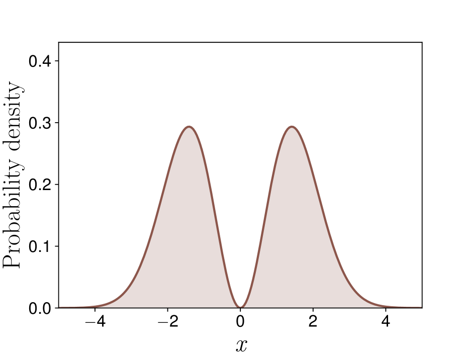
(b) L-distribution

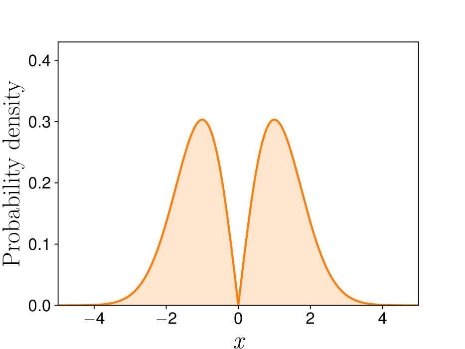
(c) B-distribution

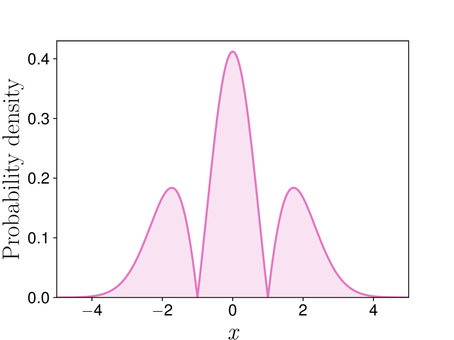
(d) W-distribution

Figure 3: Slice ratio sampling method Fig. 3(a), and new importance sampling distributions to reduce LR gradient variance (Figs. 3(b),3(c),3(d)). The shaded regions are histograms generated with the direct sampling methods, and the solid lines are the analytic densities. Both methods match, demonstrating the correctness of the derivations. B and W distributions are optimal for $\frac{\textup{d}\hfill}{\textup{d}\mu\hfill}$ and $\frac{\textup{d}\hfill}{\textup{d}\sigma\hfill}$ respectively.

Slice ratio sampling for the symmetric Beta distribution:

The slice ratio sampling method is crucial in some situations. For example, consider a distribution, such as the symmetric Beta distribution:

$$p_{\beta}\left(x\right)=\frac{x^{\alpha-1}(1-x)^{\alpha-1}}{B(\alpha,\alpha)}.$$ (7)

When $\alpha$ tends to 1 from above, this distribution tends to the uniform distribution between 0 and 1. Consider a distribution with the same shape, but where the mean is shifted, s.t. it is symmetric about a parameter $\mu$, instead of $x=\nicefrac{{1}}{{2}}$. In this case, as $\alpha$ tends to 1, the variance of the gradient w.r.t. $\mu$ will tend to $\infty$, because $\frac{\textup{d}p_{\beta}\left(x\right)\hfill}{\textup{d}\mu\hfill}$ is around 0 in most of the sampling range, but very large at the edges of the distribution. We derived the optimal pdf, sampling method and gradient estimator (App. E.3):

$$p_{\beta R}\left(x\right)=\frac{\alpha-1}{2\times 0.25^{\alpha-1}}(x-x^{2})^{\alpha-2}|1-2x|,$$ (8)

$$x=0.5\pm 0.5\sqrt{1-\epsilon_{h}^{\nicefrac{{1}}{{(\alpha-1)}}}}~{}~{}~{}\textup{where}~{}~{}~{}\epsilon_{h}\sim\textup{unif}(0,1),$$

$$\frac{\textup{d}\hfill}{\textup{d}\mu\hfill}\mathbb{E}_{x\sim p_{\beta}\left(x\right)}\left[\phi(x)\right]$$

$$=\mathbb{E}_{x\sim q(x)}\left[\textup{sgn}(x-0.5)\frac{2\times 0.25^{\alpha-1}}{B(\alpha,\alpha)}\phi(x)\right],\textup{for }\alpha>1.$$

For a shifted, stretched and centered distribution, replace $x$ with $k(x-0.5)+\mu$, and the gradient estimator needs to be scaled down by $k$. To obtain a variance $\sigma^{2}$, set $k$ to $2\sigma\sqrt{2\alpha+1}$.

Multidimensional case:

For a Gaussian $p\left(x;\theta\right)$, as the dimension increases, the optimal $q(x)$ tends to the original distribution (App. E.5). For this reason, we propose to sample each dimension separately from the B-distribution, potentially allowing for a bias, but while reducing the variance of the gradient estimator (see also App. F.1 for more justification). In general, we believe that such a technique will be necessary for other distributions as well if the dimension grows high. To see this, consider the importance weighted likelihood ratio gradient estimator for a factorized distribution $p\left({\bf x};\theta\right)=\prod_{i}p_{i}\left(x_{i};\theta_{i}\right)$:

$$\frac{\textup{d}\hfill}{\textup{d}\theta_{i}\hfill}\mathbb{E}_{{\bf x}\sim p\left({\bf x}\right)}\left[\phi({\bf x})\right]$$ (9)

$$=\mathbb{E}_{{\bf x}\sim q({\bf x})}\left[\frac{p\left({\bf x}\right)}{q({\bf x})}\frac{\textup{d}\log p\hfill}{\textup{d}\theta_{i}\hfill}\phi({\bf x})\right]$$

$$=\mathbb{E}_{{\bf x}\sim q({\bf x})}\left[\frac{p_{\backslash i}\left({\bf x}_{\backslash i}\right)p_{i}\left(x_{i}\right)}{q_{\backslash i}({\bf x}_{\backslash i})q_{i}(x_{i})}\frac{\textup{d}\log p_{i}\left(x_{i}\right)\hfill}{\textup{d}\theta_{i}\hfill}\phi({\bf x})\right],$$

$$~{}~{}~{}~{}~{}~{}~{}~{}~{}~{}~{}~{}~{}~{}\textup{where }p_{\backslash i}\textup{ is }\prod_{j\neq i}p_{j}\left(x_{j};\theta_{j}\right).$$

While $q$ can be modified to reduce the variance of $\frac{p_{i}\left(x_{i}\right)}{q_{i}(x_{i})}\frac{\textup{d}\log p_{i}\left(x_{i}\right)\hfill}{\textup{d}\theta\hfill}$, this will increase the variance of the $\frac{p_{\backslash j}\left({\bf x}_{\backslash j}\right)}{q_{\backslash j}({\bf x}_{\backslash j})}$ terms for $j\neq i$. If each $q_{j}$ is modified, then the variance of these terms grows exponentially with the dimension, and any decrease in variance from having modified $q_{i}$ becomes negligible. Our proposed solution is to replace $\frac{p_{\backslash j}\left({\bf x}_{\backslash j}\right)}{q_{\backslash j}({\bf x}_{\backslash j})}$ with its expected value, which is 1. Note that our technique is not just a convenience, but it is a necessity. In practice, such a scheme may introduce a small bias, but drastically reduce the variance. Next we show some fairly general conditions under which this method still gives an unbiased gradient estimator.

Sufficient conditions for an unbiased gradient estimator in high dimensions with our scheme:

1. If $\phi({\bf x})=\sum_{i=1}^{D}\phi_{i}(x_{i})$, then our estimation scheme is unbiased.

2. If $\phi({\bf x})$ is quadratic, then our estimation is scheme is unbiased.

Both conditions are independently sufficient for unbiasedness (derivations in App. E.6).

Effect of greater variance of $q_{i}$:

Lastly, we point toward another issue with modifying $q_{i}$ in Eq. (9). The variance of $q_{i}$ may be larger than the variance of $p_{i}$, and this could manifest as a larger variance of $\phi({\bf x})$, which would act as additional noise on the other dimensions $j\neq i$. Our proposed solution is to optimize the reduction in gradient variance while constraining the variance of $q$. Assuming the mean $\mu=0$, this can be performed using a variational optimization with an additional Lagrange multiplier for $\int q(x)x^{2}\textup{d}x=k\sigma^{2}$ analogously to Eq. (5). The general equation is

$$q(x)=\left|\frac{\textup{d}p\left(x;\theta\right)\hfill}{\textup{d}\theta\hfill}\right|/\sqrt{\lambda_{1}+\lambda_{2}x^{2}}.$$ (10)

For a Gaussian $p\left(x;\theta\right)$, this equation can be solved (App. G). We call the result the truncated ratio gradient (TRRG). The pdf, sampling method and gradient estimator are below:

$$p_{tr}\left(x;c,\mu,\sigma\right)$$ (11)

$$=\frac{\exp(-\frac{c^{2}}{2})}{1-\Phi(c)}\frac{1}{\sigma 2\sqrt{2\pi}}\frac{|x-\mu|}{\sqrt{(x-\mu)^{2}+\sigma^{2}c^{2}}}\exp(-\frac{(x-\mu)^{2}}{2\sigma^{2}})$$

$$\textup{where}~{}\Phi(c)\textup{ is the cdf of a unit normal distribution},$$

$$x=\mu\pm\sigma\sqrt{\epsilon_{c}^{2}-c^{2}}~{}~{}~{}\textup{where}~{}~{}~{}\epsilon_{c}\sim\textup{truncG}(c,\infty),\textup{and}$$

$$\textup{truncG}(a,b)\textup{ is the unit normal truncatedbetween }[a,b]$$

$$\frac{\textup{d}\hfill}{\textup{d}\mu\hfill}\mathbb{E}_{x\sim p\left(x\right)}\left[\phi(x)\right]$$

$$=\mathbb{E}_{x\sim q(x)}\left[\textup{sgn}(x-\mu)\frac{2\epsilon_{c}}{\sigma}\frac{1-\Phi(c)}{\exp(-\frac{c^{2}}{2})}\phi(x)\right].$$

This distribution interpolates between a Gaussian distribution and the B-distribution. The interpolation is controlled by the $c$ parameter: for $c=0$ the distribution is Gaussian, and for $c\rightarrow\infty$ the distribution tends to the B-distribution. One half of the distribution is plotted in Fig. 4(b) for several values of $c$, and Fig. 4(a) shows how the accuracy of $\frac{\textup{d}p\hfill}{\textup{d}\mu\hfill}/q$, and the variance of the distribution scale with $c$ (we name these functions $t(c)$ and $v(c)$ respectively). These functions were computed analytically (App. G). How should one pick the parameter $c$? A simple choice may be to pick $c$ around $0.5$, where the accuracy starts increasing slower than the variance of the distribution. But is there a more principled method based on the dimensionality?

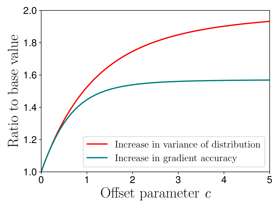
(a) $t(c)$ in teal and $v(c)$ in red

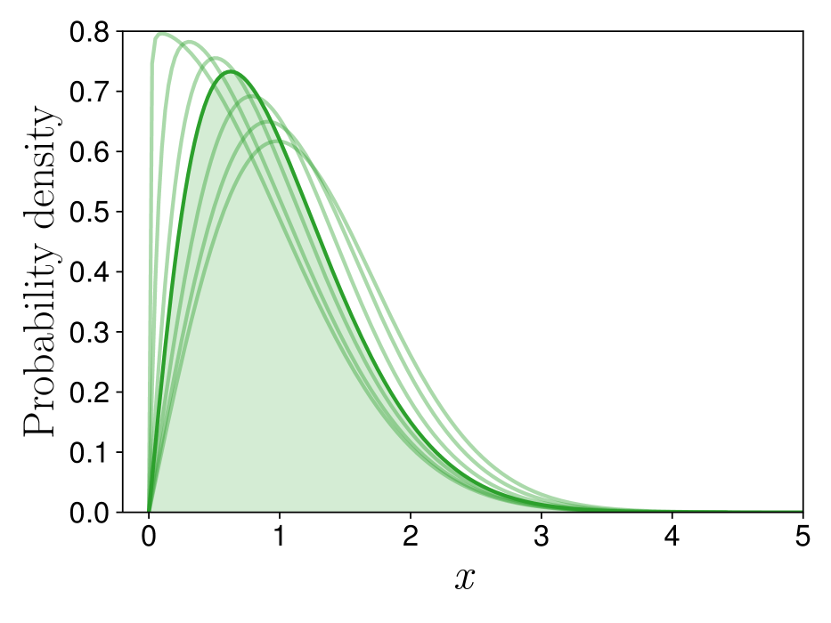
(b) $c\in[0.01,0.1,0.3,{\bf 0.5},1.0,2.0,5.0]$

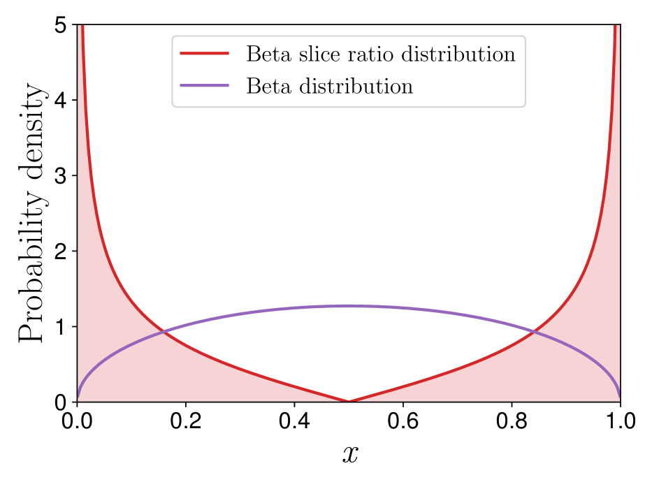
(c) $\alpha=1.5$

Figure 4: Scaling of truncated ratio gradient accuracy with the dimension (4(a)), truncated ratio distribution for various $c$ (4(b)) and the slice ratio distribution for the Beta distribution (4(c)).

Table 1: Guidelines for choosing the offset parameter $c$ for the truncated ratio gradient.

Suggested parameter $c$	0.1	0.2	0.3	0.4	0.5	0.6	0.8	1.0
Dimension $(D-1)$	4523	676	238	119	71	48	27	19
Exp. increase in accuracy $t$	1.076	1.144	1.204	1.257	1.302	1.341	1.402	1.447

We give a short analysis of the effect of the variance and guidelines for picking $c$. For example, consider the case when $\phi$ is linear with slope $a$ in every dimension, the dimensionality is $D$ and the variance is scaled by $v_{c}$, then the variance of $\phi$ would increase by a factor $v_{c}$ to $a^{2}\sigma^{2}Dv_{c}$. The noise from the other dimensions would scale as roughly $v_{c}(D-1)a^{2}\sigma^{2}$. However, the increase in accuracy $t_{c}$ counteracts this increase in noise, and the gradient variance of this noise scales as $(\nicefrac{{v_{c}}}{{t_{c}}})(D-1)a^{2}\sigma^{2}$. Now if we assume that the gradient signal has a variance around $a^{2}\sigma^{2}$, and we want to guarantee that the additional gradient noise from the other dimensions does not exceed the maximum decrease in variance, then we could pick $c$ s.t. $(\nicefrac{{v_{c}}}{{t_{c}}}-1)(D-1)\approx 1$. In Tab. 1, we show several values of $1/(\nicefrac{{v_{c}}}{{t_{c}}}-1)$ and the expected increase in accuracy $t_{c}$, which can be used as a guideline for picking an appropriate $c$ for the dimensionality of your problem. We could also estimate the reduction in gradient signal variance as $(1-\nicefrac{{1}}{{t_{c}}})a^{2}\sigma^{2}$ for a more conservative estimate of $D$, but in practice, the reduction in gradient signal variance is greater than $\nicefrac{{1}}{{t_{c}}}$ because of structure in $\phi$. In general, for deterministic problems it may be better to be conservative and aim for a smaller increase in accuracy with a smaller $c$, whereas if $\phi$ is stochastic, then the additional variance from other dimensions may be negligible and higher $c$ values can be used.

5 Experiments to verify theory

We performed experiments on a quadratic $\phi({\bf x})$ to verify the theory. In App. H we also evaluate our methods in evolution strategies experiments in reinforcement learning, but as our work proved that importance sampling for Gaussian base distributions can only lead to modest gains at best, it is difficult to obtain statistically significant results. On the other hand, our method was crucial for obtaining competitive results using a Beta distribution, as emphasized by our experiment here.

Setup:

$\phi({\bf x})$ is a quadratic $({\bf x}-{\bf a})^{T}Q({\bf x}-{\bf a})$, where ${\bf a}={\bf 1}$ and $Q=\textup{ones}(D,D)/D^{2}$ is a matrix of ones, which is scaled, such that $\phi({\bf x})$ remains constant at ${\bf x}={\bf 0}$. We evaluate a deterministic case, as well as a case when Gaussian noise $\sigma_{n}^{2}=1$ is added on $\phi$. We vary the dimension between 1–1000, and plot the variance of the gradient estimators: GLR—LR gradient with a Gaussian $p(x)$; SLRG—slice ratio gradient with a Gaussian $p(x)$; TRRG—truncated ratio gradient with $c=0.5$; BRG—slice ratio gradient with a Beta $p(x)$, and $\alpha=1.5$, plotted in Fig. 4(c); BLR—LR gradient with a Beta $p(x)$, and $\alpha=1.5$. The mean of the distributions was set to $0$ and the variance was set to $1$ (the Beta distributions were stretched by $k=2\sigma\sqrt{2\alpha+1}$ to achieve this). We used antithetic sampling, so that the effect of any baseline could be ignored. The gradient was estimated by averaging 100 samples, and this was repeated for a large number of times to estimate the variance of the gradient estimator. Bootstrapping was used to obtain confidence intervals. The results are plotted in Fig. 5.

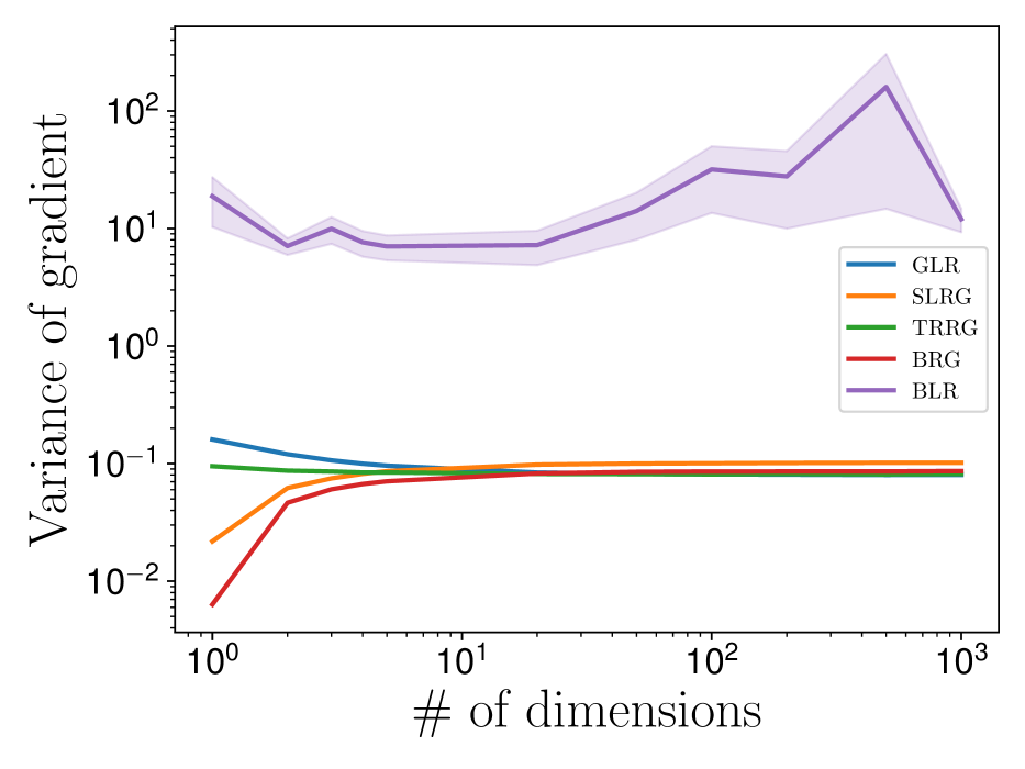
(a) Deterministic

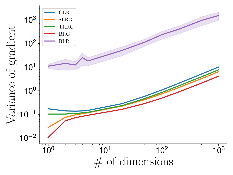
(b) Noisy

Figure 5: Scaling of gradient estimator variance on a quadratic problem with deterministic and noisy function evaluations. The confidence intervals correspond to one standard deviation of the estimate.

Results and analysis:

The main result is that using the slice ratio method, the gradient accuracy for the Beta distribution could be increased by 100–1000 times (compare BRG to BLR), showing that our method is necessary for some non-Gaussian distributions. In general, the increase in gradient accuracy would tend to $\infty$ as the $\alpha$ parameter tends to 1 from above; however, even for moderately curved cases, such as $\alpha=1.5$ (Fig. 4(c)) the improvement in accuracy can be drastic.

The results confirm our theoretical analysis: in the deterministic case, the SLRG method outperforms the standard GLR method, but as the dimensionality is increased, this reverses; whereas in the high-noise case, SLRG always outperforms GLR. In the noisy case, the gradient variances at $D=1000$ are GLR: $10.10\pm 0.05$, SLRG: $6.46\pm 0.03$, TRRG: $7.73\pm 0.04$, BRG: $4.14\pm 0.02$ (the errorbars correspond to 1 standard deviation). The ratios $10.10/6.46=1.563$ and $10.10/7.73=1.307$ match the theoretical improvements in gradient accuracy for the SLRG gradient at large $c$ in Fig. 4(a) and for the TRRG gradient at $c=0.5$ in Tab. 1. In the deterministic case, the gradient variances at $D=1000$ are GLR: $0.0803\pm 0.0004$, SLRG: $0.1015\pm 0.0005$, TRRG: $0.0815\pm 0.0004$, BRG: $0.0864\pm 0.0004$, showing that TRRG is more robust than SLRG to problems arising from increasing the dimension, while it still allows reducing the variance in the stochastic $\phi$ setting. Interestingly, BRG achieved a lower gradient variance than SLRG in the deterministic setting, and was overall the best in the stochastic setting even though the variances of the base distributions were the same.

6 Conclusions

We have introduced a new unified theory of LR and RP gradients. The theory explained that the sampling distribution $q(x)$ for LR gradients is a separate matter to the distribution $p(x;\theta)$ used to compute the objective function $\mathbb{E}_{x\sim p\left(x;\theta\right)}\left[\phi(x)\right]$, and motivated us to search for the optimal importance sampling distribution $q(x)$ to reduce gradient variance. We derived these importance sampling distributions together with sampling methods for them for Gaussian and Beta objective distributions $p\left(x;\theta\right)$ to reduce the variance of the gradient w.r.t. a mean shifting parameter of the distribution. Optimal sampling for other gradients is left for future work. We further analyzed the scalability with the dimension of the sampling space. Gaussian distributions are widely used in the literature, and we found that our method is able to provide a modest improvement in gradient accuracy. On the other hand, for distributions with a “flat top”, which have found less use, our method can drastically improve the accuracy, and is crucial for obtaining good results. Which objective distributions outperform Gaussians in which situations is a substantial research topic: e.g. clipped distributions (Fujita and Maeda,, 2018), Beta distributions (Chou et al.,, 2017), exponential family distributions (Eisenach and Yang,, 2019) or normalizing flows (Tang and Agrawal,, 2018; Mazoure et al.,, 2019) have been considered, but they did not importance sample from $q(x)$. Our slice ratio gradients will be essential to obtain a fair comparison between different $p\left(x;\theta\right)$.

Acknowledgments

PP was supported by OIST Graduate School funding and by RIKEN. MS was supported by KAKENHI 17H00757.

Appendix A Likelihood ratio gradient basics

The likelihood ratio (LR) gradient estimator is given by

$$\frac{\textup{d}\hfill}{\textup{d}\theta\hfill}\mathbb{E}_{x\sim p\left(x;\theta\right)}\left[\phi(x)\right]=\mathbb{E}_{x\sim p\left(x;\theta\right)}\left[\frac{\textup{d}\log p\left(x;\theta\right)\hfill}{\textup{d}\theta\hfill}\phi(x)\right].$$ (12)

For a Gaussian $p\left(x;\theta\right)$:

$$\log p\left(x;\theta\right) =-\frac{1}{2}\log(2\pi)-\log(\sigma)-\frac{(x-\mu)^{2}}{2\sigma^{2}},$$ (13)

$$\frac{\textup{d}\log p\left(x;\theta\right)\hfill}{\textup{d}\mu\hfill} =\frac{x-\mu}{\sigma^{2}}=\frac{\epsilon}{\sigma},$$

$$\frac{\textup{d}\log p\left(x;\theta\right)\hfill}{\textup{d}\sigma\hfill} =\frac{(x-\mu)^{2}}{\sigma^{3}}-\frac{1}{\sigma}=\frac{\epsilon^{2}}{\sigma}-\frac{1}{\sigma},$$

where $$x=\mu+\epsilon\sigma\textup{ and }\epsilon\sim\mathcal{N}(0,1).$$

For a Beta $p\left(x;\theta\right)$:

$$p\left(x;\theta\right) =\frac{(x-x^{2})^{\alpha-1}}{B(\alpha,\alpha)}~{}~{}\textup{for }x\in[0,1]$$ (14)

$$\log p\left(x;\theta\right) =-\log\left(B(\alpha,\alpha)\right)+(\alpha-1)\log(x-x^{2}),$$

$$\frac{\textup{d}\log p\left(x;\theta\right)\hfill}{\textup{d}x\hfill} =\frac{\alpha-1}{x-x^{2}}(1-2x),$$

$$\frac{\textup{d}\log p\left(x;\theta\right)\hfill}{\textup{d}\mu\hfill} =-\frac{\textup{d}\log p\left(x;\theta\right)\hfill}{\textup{d}x\hfill},~{}~{}$$

$$\textup{where }\mu$$ is a shifting parameter for the mean.

In practice, we sample an $\epsilon_{\beta}=x-0.5\Rightarrow x=\epsilon_{\beta}+0.5$, then the gradient estimator becomes: $\frac{2\epsilon_{\beta}(\alpha-1)}{0.25-\epsilon_{\beta}^{2}}\frac{1}{k}$, where the additional $k$ factor comes if a stretching is applied: $z=\mu+k\epsilon_{\beta}$.

Baselines to reduce gradient variance:

The LR gradient estimator on its own has a large variance, and techniques have to be used to stabilize it. A common technique is to subtract a constant baseline $b$ from the $\phi(x)$ values, so that the gradient estimator becomes

$$\frac{\textup{d}\hfill}{\textup{d}\theta\hfill}\mathbb{E}_{x\sim p\left(x;\theta\right)}\left[\frac{\textup{d}\log p\left(x;\theta\right)\hfill}{\textup{d}\theta\hfill}\left(\phi(x)-b\right)\right].$$ (15)

In practice, using $b=\mathbb{E}_{x\sim p\left(x;\theta\right)}\left[\phi(x)\right]$ works well, but one can also derive an optimal baseline (Weaver and Tao,, 2001). We outline the derivation below. The gradient variance when a baseline is used can be expressed as

$$\mathbb{V}_{x\sim p\left(x;\theta\right)}\left[\frac{\textup{d}\log p\left(x;\theta\right)\hfill}{\textup{d}\theta\hfill}\left(\phi(x)-b\right)\right] =~{}~{}\mathbb{E}_{x\sim p\left(x;\theta\right)}\left[\left(\frac{\textup{d}\log p\left(x;\theta\right)\hfill}{\textup{d}\theta\hfill}\phi(x)\right)^{2}\right]$$ (16)

$$-2\mathbb{E}_{x\sim p\left(x;\theta\right)}\left[\left(\frac{\textup{d}\log p\left(x;\theta\right)\hfill}{\textup{d}\theta\hfill}\right)^{2}\phi(x)b\right]+\mathbb{E}_{x\sim p\left(x;\theta\right)}\left[\left(\frac{\textup{d}\log p\left(x;\theta\right)\hfill}{\textup{d}\theta\hfill}b\right)^{2}\right].$$

Taking the derivative of Eq. (16) w.r.t. $b$ and setting to zero gives the optimal baseline as

$$b_{opt}=\frac{\mathbb{E}_{x\sim p\left(x;\theta\right)}\left[\left(\frac{\textup{d}\log p\left(x;\theta\right)\hfill}{\textup{d}\theta\hfill}\right)^{2}\phi(x)\right]}{\mathbb{E}_{x\sim p\left(x;\theta\right)}\left[\left(\frac{\textup{d}\log p\left(x;\theta\right)\hfill}{\textup{d}\theta\hfill}\right)^{2}\right]}.$$ (17)

In practice, for example if $\phi(x)$ is linear and $p\left(x;\theta\right)$ is Gaussian then $b_{opt}=\mathbb{E}_{x\sim p\left(x;\theta\right)}\left[\phi(x)\right]$, so the gain from trying to use an optimal baseline is often small. What would happen to the optimal baseline derivation for our importance sampling case (Sec. 4)? The sampling distribution has to be swapped with $q(x)$, and $\frac{\textup{d}\log p\left(x;\theta\right)\hfill}{\textup{d}\theta\hfill}$ has to be swapped with $\nicefrac{{\frac{\textup{d}p\left(x;\theta\right)\hfill}{\textup{d}\theta\hfill}}}{{q(x)}}$, giving the optimal baseline (Jie and Abbeel,, 2010) as

$$b_{opt}=\frac{\mathbb{E}_{x\sim q(x)}\left[\left(\nicefrac{{\frac{\textup{d}p\left(x;\theta\right)\hfill}{\textup{d}\theta\hfill}}}{{q(x)}}\right)^{2}\phi(x)\right]}{\mathbb{E}_{x\sim q(x)}\left[\left(\nicefrac{{\frac{\textup{d}p\left(x;\theta\right)\hfill}{\textup{d}\theta\hfill}}}{{q(x)}}\right)^{2}\right]}.$$ (18)

Note that if the slice ratio distribution is used, then $q=\left|\frac{\textup{d}p\left(x;\theta\right)\hfill}{\textup{d}\theta\hfill}\right|/\sqrt{\lambda}$, and $b_{opt}=\mathbb{E}_{x\sim q(x)}\left[\phi(x)\right]$.

Antithetic sampling:

An often used technique is to sample points $x$ in pairs opposite to each other, s.t. $x_{+}=\mu+\sigma\epsilon$ and $x_{-}=\mu-\sigma\epsilon$. This technique is particularly often used in evolution strategies’ research (Salimans et al.,, 2017; Mania et al.,, 2018). We will explain that when this technique is used, then a baseline has no effect because it cancels. Thus, using antithetic sampling allows us to disentangle any effect of the baselines from the effect of the importance sampling, which is why we use it in all of our experiments. The derivation is easy to see by considering that for a Gaussian: $\frac{\textup{d}\log p\left(x;\theta\right)\hfill}{\textup{d}\mu\hfill}=\frac{\epsilon}{\sigma}$, so $\frac{\textup{d}\log p\left(x_{+};\theta\right)\hfill}{\textup{d}\mu\hfill}(\phi(x_{+})-b)+\frac{\textup{d}\log p\left(x_{-};\theta\right)\hfill}{\textup{d}\mu\hfill}(\phi(x_{-})-b)=\frac{\epsilon}{\sigma}\left(\phi(x_{+})-b-(\phi(x_{-})-b)\right)=\frac{\epsilon}{\sigma}\left(\phi(x_{+})-\phi(x_{-})\right)$. In general, this result holds for any symmetric $\nicefrac{{\frac{\textup{d}p\left(x;\theta\right)\hfill}{\textup{d}\theta\hfill}}}{{q(x)}}$.

Relationship to finite difference methods:

Finite difference methods also use the function values $\phi(x)$ to estimate a derivative, so it may appear that the LR gradient estimator is a finite difference estimator. Finite difference estimators work by estimating the slope of the function, by evaluating the change between two points, i.e.

$$\frac{\textup{d}\phi(x)\hfill}{\textup{d}x\hfill}\approx\frac{\phi(x_{+})-\phi(x_{-})}{\Delta x}.$$ (19)

In the antithetic sampling case, $\Delta x=2\sigma\epsilon$, so the estimator is

$$\frac{\textup{d}\phi(x)\hfill}{\textup{d}x\hfill}\approx\frac{\phi(x_{+})-\phi(x_{-})}{2\sigma\epsilon}.$$ (20)

Clearly, this is different to the LR gradient estimator

$$\frac{\epsilon\left(\phi(x_{+})-\phi(x_{-})\right)}{2\sigma},$$ (21)

because the $\epsilon$ is in the wrong place. In Sec. 2 we explain that the LR gradient estimator is a different concept to finite differences, which is not trying to fit a linear function onto $\phi(x)$.

Appendix B Derivations for the probability flow theory

Here we illustrate the background information in 3 dimensions, but it generalizes straightforwardly to higher dimensions.

Notation:

${\bf F}=[F_{x}(x,y,z),F_{y}(x,y,z),F_{z}(x,y,z)]$ is a vector field.
$\phi(x,y,z)$ is a scalar field (a scalar function)
Div operator: $\nabla\cdot{\bf F}=\frac{\partial F_{x}}{\partial x}+\frac{\partial F_{y}}{\partial y}+\frac{\partial F_{z}}{\partial z}$.
Grad operator: $\nabla\phi=[\frac{\partial\phi}{\partial x},\frac{\partial\phi}{\partial y},\frac{\partial\phi}{\partial z}]$.

B.1 Basic vector calculus and fluid mechanics

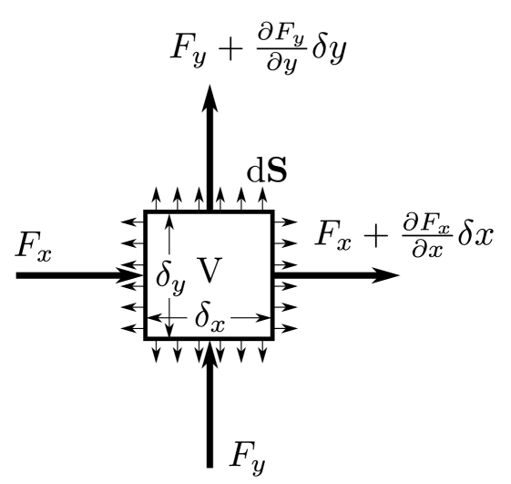
Figure 6: Illustration of the divergence theorem.

The vector field ${\bf F}$ could be for example thought of as a local flow velocity for some fluid. If ${\bf F}$ is the density flow rate, then the div operator essentially measures how much the density is decreasing at a point. If the outflow is larger than the inflow, the density would decrease and vice versa. The divergence theorem, illustrated in Fig. 6 illustrates how this change in density can be measured in two separate ways: one could integrate the divergence across the volume, or one could integrate the in and and outflow across the surface. The divergence theorem states:

$$\int_{V}\nabla\cdot{\bf F}\textup{d}V=\int_{S}{\bf F}\cdot\textup{d}{\bf S}$$ (22)

To prove the claim, consider the infinitesimal box in Fig. 6. The divergence can be calculated as $\delta x\delta y(\frac{\partial F_{x}}{\partial x}+\frac{\partial F_{y}}{\partial y})$. On the other hand, to take the integral across the surface, note that the surface normals point outwards, and the integral becomes $\delta_{y}(-F_{x}+F_{x}-\frac{\partial F_{x}}{\partial x}\delta x)+\delta x(-F_{y}+F_{y}+\frac{\partial F_{y}}{\partial y}\delta y)=\delta x\delta y(\frac{\partial F_{x}}{\partial x}+\frac{\partial F_{y}}{\partial y})$, which is the same as the divergence. To generalize this to arbitrarily large volumes, notice that if one stacks the boxes next to each other, then the surface integral across the area where the boxes meet cancels out, and only the integral across the outer surface remains. For an incompressible flow, the density does not change, and the divergence must be zero.

B.2 Derivation of probability surface integral

We will show that the LR estimator tries to integrate $\int_{S}\phi(\tilde{{\bf x}})\nabla_{\theta}\tilde{g}(\epsilon_{x},\epsilon_{h})\textup{d}{\bf S}$. First, note that $\textup{d}{\bf S}=\hat{{\bf n}}\textup{d}S$, and it is necessary to express the normalized surface vector $\hat{{\bf n}}$. To do so, we first express the tangent vector ${\bf t}$, then change the height component of this vector to obtain a vector perpendicular to the tangent vector (this is exactly the normal vector).

A vector tangent and downhill to the surface is given by ${\bf t}=[-\frac{\textup{d}p\hfill}{\textup{d}{\bf x}\hfill},-\left(\frac{\textup{d}p\hfill}{\textup{d}{\bf x}\hfill}\right)\left(\frac{\textup{d}p\hfill}{\textup{d}{\bf x}\hfill}\right)^{T}]$. The normal vector ${\bf n}$ is $[-\frac{\textup{d}p\hfill}{\textup{d}{\bf x}\hfill};h]$, such that ${\bf t}\cdot{\bf n}=0$. Therefore, $\left(\frac{\textup{d}p\hfill}{\textup{d}{\bf x}\hfill}\right)\left(\frac{\textup{d}p\hfill}{\textup{d}{\bf x}\hfill}\right)^{T}-\left(\frac{\textup{d}p\hfill}{\textup{d}{\bf x}\hfill}\right)\left(\frac{\textup{d}p\hfill}{\textup{d}{\bf x}\hfill}\right)^{T}h=0~{}~{}\Rightarrow~{}~{}h=1$. Finally, we normalize the vector:

$$\hat{{\bf n}}=\nicefrac{{[-\frac{\textup{d}p\hfill}{\textup{d}{\bf x}\hfill},1]}}{{\sqrt{\left(\frac{\textup{d}p\hfill}{\textup{d}{\bf x}\hfill}\right)\left(\frac{\textup{d}p\hfill}{\textup{d}{\bf x}\hfill}\right)^{T}+1}}}~{}.$$ (23)

Next, we perform a change of coordinates from the surface elements $\textup{d}S$ to cartesian coordinates $\textup{d}{\bf x}$. When projecting a surface element $\textup{d}S$ with unit normal $\hat{{\bf n}}$ to a plane with unit normal $\hat{{\bf m}}$, the projected area is given by $\textup{d}{\bf x}=\left|\hat{{\bf n}}\cdot\hat{{\bf m}}\right|\textup{d}S$, therefore $\textup{d}{\bf x}=\textup{d}S\left|\frac{1}{\sqrt{\left(\frac{\textup{d}p\hfill}{\textup{d}{\bf x}\hfill}\right)\left(\frac{\textup{d}p\hfill}{\textup{d}{\bf x}\hfill}\right)^{T}+1}}[-\frac{\textup{d}p\hfill}{\textup{d}{\bf x}\hfill},1]\cdot[{\bf 0},1]\right|=\nicefrac{{\textup{d}S}}{{\sqrt{\left(\frac{\textup{d}p\hfill}{\textup{d}{\bf x}\hfill}\right)\left(\frac{\textup{d}p\hfill}{\textup{d}{\bf x}\hfill}\right)^{T}+1}}}$, from which we get

$$\textup{d}S=\sqrt{\left(\frac{\textup{d}p\hfill}{\textup{d}{\bf x}\hfill}\right)\left(\frac{\textup{d}p\hfill}{\textup{d}{\bf x}\hfill}\right)^{T}+1}~{}~{}\textup{d}{\bf x}.$$ (24)

Plugging Eqs. (23) and (24) into the right-hand side of Eq. (3) we get

$$\int_{X}\phi(\tilde{{\bf x}})\nabla_{\theta}\tilde{g}(\epsilon_{x},\epsilon_{h})\cdot\frac{[-\frac{\textup{d}p\hfill}{\textup{d}{\bf x}\hfill},1]}{\sqrt{\left(\frac{\textup{d}p\hfill}{\textup{d}{\bf x}\hfill}\right)\left(\frac{\textup{d}p\hfill}{\textup{d}{\bf x}\hfill}\right)^{T}+1}}\sqrt{\left(\frac{\textup{d}p\hfill}{\textup{d}{\bf x}\hfill}\right)\left(\frac{\textup{d}p\hfill}{\textup{d}{\bf x}\hfill}\right)^{T}+1}~{}~{}\textup{d}{\bf x} =$$ (25)

$$\int_{X}\phi(\tilde{{\bf x}})\nabla_{\theta}\tilde{g}(\epsilon_{x},\epsilon_{h}) \cdot[-\frac{\textup{d}p\hfill}{\textup{d}{\bf x}\hfill},1]~{}\textup{d}{\bf x}.$$

Recall that the last element of $\tilde{g}(\epsilon_{x},\epsilon_{h})$ is $\epsilon_{h}p\left(g(\epsilon_{x});\theta\right)$, and that $\epsilon_{h}$ at the boundary surface is $1$, then the $\nabla_{\theta}\tilde{g}(\epsilon_{x},\epsilon_{h})\cdot[-\frac{\textup{d}p\hfill}{\textup{d}{\bf x}\hfill},1]$ term turns into $-\nabla_{\theta}g(\epsilon_{x})\cdot\frac{\textup{d}p\hfill}{\textup{d}{\bf x}\hfill}+\left.\frac{\partial\epsilon_{h}p\left(g(\epsilon_{x});\theta\right)}{\partial\theta\hfill}\right|_{\epsilon_{x}=const,\epsilon_{h}=1}$. The last term $\left.\frac{\partial p\left(g(\epsilon_{x});\theta\right)}{\partial\theta\hfill}\right|_{\epsilon_{x}=const}$ can be thought of as the rate of change of the probability density while following a point moving in the flow induced by perturbing $\theta$. This quantity can be expressed with the material derivative $\left.\frac{\partial p\left(g(\epsilon_{x});\theta\right)}{\partial\theta\hfill}\right|_{\epsilon_{x}=const}=\frac{\textup{d}p\left({\bf x};\theta\right)\hfill}{\textup{d}\theta\hfill}+\nabla_{\theta}g(\epsilon_{x})\cdot\frac{\textup{d}p\hfill}{\textup{d}{\bf x}\hfill}$. Finally, substituting into Eq. (25):

$$\int_{S}\phi(\tilde{{\bf x}})\nabla_{\theta}\tilde{g}(\epsilon_{x},\epsilon_{h})~{}\textup{d}{\bf S}=\int_{X}\phi({\bf x})\frac{\textup{d}p\left({\bf x};\theta\right)\hfill}{\textup{d}\theta\hfill}~{}\textup{d}{\bf x}.$$ (26)

Appendix C Reparameterization gradients are not unique

What happens if we perform the same kind of analysis as in Theorem 1 for the RP gradient? Similarly, suppose that there exist $u({\bf x})$ and $v({\bf x})$, s.t. $\int\nabla\phi({\bf x})\cdot u({\bf x})~{}\textup{d}{\bf x}=\int\nabla\phi({\bf x})\cdot v({\bf x})~{}\textup{d}{\bf x}$ for any $\phi({\bf x})$. Rearrange the equation into $\int\nabla\phi({\bf x})\cdot\left(u({\bf x})-v({\bf x})\right)~{}\textup{d}{\bf x}=0$. Then, if we can pick $\nabla\phi({\bf x})=u({\bf x})-v({\bf x})$ it would lead to $u=v$, which would show the uniqueness. However, it is not necessarily possible to pick such $\phi({\bf x})$. In particular, the integral of $\nabla\phi({\bf x})$ over any closed path is 0, but this is not necessarily the case for $u-v$. Therefore, the same kind of analysis does not lead to a claim of uniqueness. Indeed, concurrent work (Jankowiak and Obermeyer,, 2018) showed that there are an infinite amount of possible reparameterization gradients, and the minimum variance is achieved by the optimal transport flow.

Appendix D Slice integral importance sampling

From Theorem 1 we saw that unlike the RP gradient case, the weighting $\psi$ for function values $\phi({\bf x})$ with ${\bf x}\sim p\left({\bf x};\theta\right)$ to obtain an unbiased estimator for the gradient $\frac{\textup{d}\hfill}{\textup{d}\theta\hfill}\mathbb{E}\left[\phi({\bf x})\right]$ is unique. The only option to reduce the variance by changing the weighting would then be to sample from a different distribution $q({\bf x})$ via importance sampling. Motivated by the resemblance of the “boxes” theory in Sec. 2 to the Riemann integral, we propose to sample horizontal slices of probability mass resembling the Lebesgue integral. Such an approach appears attractive, because if the location of the slice is moved by modifying the parameters of the distribution (e.g., by changing the mean), then the derivative of the expected value of the integral over the slice will depend only on the value at the edges of the slice (because the probability density in the middle would not change). To obtain the gradient estimator, it will only be necessary to compute the probability density $p_{L}\left({\bf x};\theta\right)$. We derive such a “slice integral” distribution corresponding to the Gaussian distribution. The method resembles the seminal work by Neal, (2003) on slice sampling in Markov chain Monte Carlo methods. We call our new distribution the L-distribution, and it is plotted in Fig. 3(b).

Derivation of the pdf of the L-distribution:

One way to sample whole slices of a probability distribution would be to sample a height $h$ between 0 and $p_{\mathrm{max}}$ proportionally to the probability mass at that height. The probability mass at a height $h$ is just given by $2|x-\mu|$ where $x$ is such that $p\left(x;\mu,\sigma\right)=h$, i.e., $2|x-\mu|$ is the distance between the edges of $p\left(x;\mu,\sigma\right)$. The probability mass corresponding to $x$ is then given by $2|x-\mu|\textup{d}h$. Performing a change of coordinates to the $x$-domain, and splitting the mass between the two edges of the slice, we get $|x-\mu|\textup{d}h=|x-\mu|\left|\frac{\textup{d}p\left(x;\mu,\sigma\right)\hfill}{\textup{d}x\hfill}\right|\textup{d}x$. This gives a closed-form normalized pdf for the L-distribution:

$$p_{L}\left(x;\mu,\sigma\right)=|x-\mu|\left|\frac{\textup{d}p\left(x;\mu,\sigma\right)\hfill}{\textup{d}x\hfill}\right| =|x-\mu|p\left(x;\mu,\sigma\right)\frac{|x-\mu|}{\sigma^{2}}$$ (27)

$$=\frac{|x-\mu|^{2}}{\sqrt{2\pi}~{}\sigma^{3}}\exp\left(\frac{-(x-\mu)^{2}}{2\sigma^{2}}\right).$$

One can recognize that Eq. (27) is actually just a Maxwell-Boltzmann distribution reflected about the origin with the probability mass split between the two sides.

Sampling from the L-distribution:

To sample from this distribution, it is necessary to sample points proportionally to the length of the slices. It suffices to sample uniformly in the area under the curve in the space augmented with the height dimension $h$, then selecting the slice on which the sampled point lies. This can be achieved with the three steps: 1) sample a point from the base distribution: $x_{s}\sim p\left(x;\mu,\sigma\right)$, 2) sample a height: $h\sim\textup{unif}\left(0,p\left(x_{s};\mu,\sigma\right)\right)$, 3) compute where the edge of slice is $x=p^{-1}(h;\mu,\sigma)$, where $p^{-1}(h)$ inverts the pdf, and computes the location $x$ that gives a probability density $h$. For the L-distribution, this can be achieved by sampling $\epsilon_{x}\sim\mathcal{N}(0,1)$ and $\epsilon_{h}\sim\textup{unif}(0,1)$ and transforming these by the equation:

$$x=\mu\pm\sigma\sqrt{-2\log(\epsilon_{h})+\epsilon_{x}^{2}}~{}.$$ (28)

Now it is straightfoward to obtain the LR gradient estimator:

$$\frac{\textup{d}\hfill}{\textup{d}\mu\hfill}\mathbb{E}_{x\sim p\left(x;\theta\right)}\left[\phi(x)\right]=\mathbb{E}_{x\sim q(x;\theta)}\left[\frac{\frac{\textup{d}p\hfill}{\textup{d}\mu\hfill}}{q(x;\theta)}\phi(x)\right] =\mathbb{E}_{x\sim q(x;\theta)}\left[\frac{1}{x-\mu}\phi(x)\right]$$ (29)

$$=\mathbb{E}\left[\frac{\textup{sgn}(x-\mu)}{\sigma\sqrt{-2\log(\epsilon_{h})+\epsilon_{x}^{2}}}\phi(x)\right].$$

Appendix E Slice ratio gradient derivations

E.1 Slice ratio gradients for general distributions

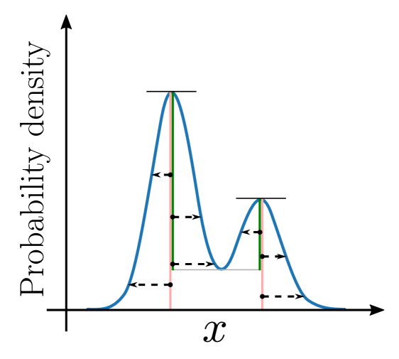
Figure 7: Slice ratio sampling method for general multimodal distributions.

So far we have introduced slice ratio gradients for unimodal distributions. Here we explain that the technique works for arbitrary distributions. The process is illustrated in Fig. 7. The curve $p\left(x;\theta\right)$ is projected onto the vertical dimension. Then one samples uniformly in this projected area, and maps the sampled points back onto the curve via $x=p^{-1}(h)$. The probability density in the $h$-space is uniformly $1/H$, where $H$ is the total length of the vertical lines. Changing coordinates will give $\textup{d}h/H=|\frac{\textup{d}p\hfill}{\textup{d}x\hfill}|\textup{d}x/H$. Thus, this sampling method will always sample proportionally to $|\frac{\textup{d}p\hfill}{\textup{d}x\hfill}|$. Because $\frac{\textup{d}p\hfill}{\textup{d}x\hfill}=-\frac{\textup{d}p\hfill}{\textup{d}\mu\hfill}$ for arbitrary distributions, this sampling method gives the desired importance sampling distribution to minimize the variance of the gradient w.r.t. $\mu$ for arbitrary distributions. The probability density becomes

$$q(x)=\frac{1}{H}\left|\frac{\textup{d}p\hfill}{\textup{d}x\hfill}\right|,$$ (30)

and the gradient estimator for one sample becomes

$$\frac{\frac{\textup{d}p\hfill}{\textup{d}\mu\hfill}}{\left|\frac{\textup{d}p\hfill}{\textup{d}\mu\hfill}\right|/H}\phi(x)=\textup{sgn}\left(\frac{\textup{d}p\hfill}{\textup{d}\mu\hfill}\right)H\phi(x).$$ (31)

E.2 Slice ratio gradient for a Gaussian distribution

The pdf is

$$p\left(x\right)=\frac{1}{\sqrt{2\pi}\sigma}\exp\left(-\frac{(x-\mu)^{2}}{2\sigma^{2}}\right).$$ (32)

The maximum probability density is at $x=\mu$:

$$p_{\mathrm{max}}=\frac{1}{\sqrt{2\pi}\sigma}.$$ (33)

The probability density for the slice ratio distribution can be derived by performing a change in coordinates from the $h$ value to $x$. The probability mass at a slice $\textup{d}h$ split between two sides is $\nicefrac{{\textup{d}h}}{{2p_{\mathrm{max}}}}$, so

$$\frac{1}{2p_{\mathrm{max}}}\textup{d}h=\frac{1}{2p_{\mathrm{max}}}\left|\frac{\textup{d}p\hfill}{\textup{d}x\hfill}\right|\textup{d}x.$$ (34)

From this we get

$$q(x) =\frac{\sqrt{2\pi}\sigma}{2}\left|\frac{1}{\sqrt{2\pi}\sigma}\exp\left(-\frac{(x-\mu)^{2}}{2\sigma^{2}}\right)\frac{-(x-\mu)}{\sigma^{2}}\right|$$ (35)

$$=\frac{\left|x-\mu\right|}{2\sigma^{2}}\exp\left(-\frac{(x-\mu)^{2}}{2\sigma^{2}}\right),$$

which is the pdf in Eq. (6).

To derive the sampling method, first derive the inverse of the probability density $p^{-1}(h)$ as

$$h =\frac{1}{\sqrt{2\pi}\sigma}\exp\left(-\frac{(x-\mu)^{2}}{2\sigma^{2}}\right)$$ (36)

$$\log(h) =-\frac{1}{2}\log(2\pi)-\log(\sigma)-\frac{(x-\mu)^{2}}{2\sigma^{2}}$$

$$(x-\mu)^{2} =-2\sigma^{2}\left(\frac{1}{2}\log(2\pi)+\log(\sigma)+\log(h)\right)$$

$$x =\mu\pm\sigma\sqrt{-\log(2\pi)-2\log(\sigma)-2\log(h)}~{}.$$

Now, noting $h=p_{\mathrm{max}}\epsilon_{h}$, where $\epsilon_{h}\sim\textup{unif}(0,1)$, we end up with the sampling method:

$$x =\mu\pm\sigma\sqrt{-\log(2\pi)-2\log(\sigma)-2\log(\frac{1}{\sqrt{2\pi}\sigma}\epsilon_{h})}$$ (37)

$$=\mu\pm\sigma\sqrt{-2\log(\epsilon_{h})}~{},\textup{where }\epsilon_{h}\sim\textup{unif}(0,1).$$

E.3 Slice ratio gradient for a symmetric Beta distribution

The pdf is

$$p_{\beta}\left(x\right)=\frac{x^{\alpha-1}(1-x)^{\alpha-1}}{B(\alpha,\alpha)}=\frac{(x-x^{2})^{\alpha-1}}{B(\alpha,\alpha)}.$$ (38)

The maximum probability density is at $x=0.5$:

$$p_{\mathrm{max}}=\frac{0.25^{\alpha-1}}{B(\alpha,\alpha)}$$ (39)

Similarly to Eq. (35), the pdf of the slice ratio distribution is $q(x)=\nicefrac{{|\frac{\textup{d}p\hfill}{\textup{d}x\hfill}|}}{{2p_{\mathrm{max}}}}$:

$$q(x) =\frac{B(\alpha,\alpha)}{2\times 0.25^{\alpha-1}}\left|\frac{(x-x^{2})^{\alpha-2}}{B(\alpha,\alpha)}(\alpha-1)(1-2x)\right|$$ (40)

$$=\frac{\alpha-1}{2\times 0.25^{\alpha-1}}\left|(x-x^{2})^{\alpha-2}(1-2x)\right|,$$

which is the pdf in Eq. (8).

To derive the sampling method, first derive the inverse of the probability density $p^{-1}(h)$ as

$$h =\frac{(x-x^{2})^{\alpha-1}}{B(\alpha,\alpha)}$$ (41)

$$h^{\nicefrac{{1}}{{(\alpha-1)}}} =\frac{(x-x^{2})}{B(\alpha,\alpha)^{\nicefrac{{1}}{{(\alpha-1)}}}}$$

$$x^{2}-x+\left(hB(\alpha,\alpha)\right)^{\nicefrac{{1}}{{(\alpha-1)}}} =0$$

$$x =\frac{1}{2}\pm\frac{1}{2}\sqrt{1-4(hB(\alpha,\alpha))^{\nicefrac{{1}}{{(\alpha-1)}}}}~{}.$$

Now, noting $h=p_{\mathrm{max}}\epsilon_{h}$, where $\epsilon_{h}\sim\textup{unif}(0,1)$, we end up with the sampling method:

$$x =\frac{1}{2}\pm\frac{1}{2}\sqrt{1-4\left(\epsilon_{h}\frac{0.25^{\alpha-1}}{B(\alpha,\alpha)}B(\alpha,\alpha)\right)^{\nicefrac{{1}}{{(\alpha-1)}}}}$$ (42)

$$=\frac{1}{2}\pm\frac{1}{2}\sqrt{1-\epsilon_{h}^{\nicefrac{{1}}{{(\alpha-1)}}}}~{},\textup{where }\epsilon_{h}\sim\textup{unif}(0,1).$$

Stretching factor k to achieve variance $\sigma^{2}$:

The variance of the Beta distribution is given by $\frac{\alpha^{2}}{(2\alpha)^{2}(2\alpha+1)}=\frac{1}{4(2\alpha+1)}$. We need $k^{2}\frac{1}{4(2\alpha+1)}=\sigma^{2}\Rightarrow k=2\sigma\sqrt{2\alpha+1}$.

E.4 W-distribution for minimizing variance of $\frac{\textup{d}\hfill}{\textup{d}\sigma\hfill}$

For completeness, for a Gaussian we also derive the optimal sampling distribution for the derivative w.r.t. $\sigma$. First note that $\frac{\textup{d}p\left(x\right)\hfill}{\textup{d}\sigma\hfill}=\sigma\frac{\textup{d}^{2}p\left(x\right)\hfill}{\textup{d}x^{2}\hfill}$. This expression means that if we apply the same height sampling concept as used for $\mu$ on the distribution proportional to $\left|\frac{\textup{d}p\left(x\right)\hfill}{\textup{d}x\hfill}\right|$, we would obtain samples with probability density proportional to $\left|\frac{\textup{d}^{2}p\left(x\right)\hfill}{\textup{d}x^{2}\hfill}\right|$, and would hence be sampling from the desired distribution. The required base distribution is just the B-distribution (Eq. (6)), so we can perform the required derivation.

The result is given below:

$$p_{W}\left(x;\mu,\sigma\right) =\frac{\sqrt{e}}{4\sigma}\left|\exp\left(\frac{-(x-\mu)^{2}}{2\sigma^{2}}\right)\left(\frac{|x-\mu|^{2}}{\sigma^{2}}-1\right)\right|,$$ (43)

$$x =\mu\pm\sigma\sqrt{W(-\epsilon_{h}^{2}/e)}~{}~{}~{}\textup{where}~{}~{}~{}\epsilon_{h}\sim\textup{unif}(0,1),$$

$$\frac{\textup{d}\hfill}{\textup{d}\sigma\hfill}\mathbb{E}_{x\sim p\left(x\right)}\left[\phi(x)\right] =\mathbb{E}_{x\sim p_{W}\left(x\right)}\left[\textup{sgn}\left(\frac{(x-\mu)^{2}}{\sigma^{2}}-1\right)\frac{2\sqrt{2}}{\sigma\sqrt{e\pi}}\phi(x)\right].$$

In the above equation, $W(x)$ is the Lambert W function (Corless et al.,, 1996)—a function s.t. $z=W(ze^{z})$. The solution for $W$ is picked with equal probability from the $-1$ and $0$ branches of $W$, and the $\pm$ is also sampled randomly with equal probability. Efficient implementations of $W$ are available in common numerical computation packages, such as scipy (Jones et al., 01, ) or MATLAB. We call the result the W-distribution, and it is plotted in Fig. 3(d). To the best of our knowledge, this distribution does not exist in the literature.

Derivation of W-distribution:

We first derive the probability density $p_{W}\left(x\right)$, then the sampling scheme. The base distribution is $p_{B}\left(x\right)$, and we apply a transformation by which we sample the height $h$, and transorm this to a point $x$ by using the inverse $x=p_{B}^{-1}(h)$, and sampling uniformly between the $x$ values that satisfy the equation, e.g. for the B-distribution in Fig. 3(c) there are usually 4 points for each $h$ value. Therefore $\textup{d}h=\frac{1}{4\textup{max}(p_{B})}\left|\frac{\textup{d}p_{B}\left(x\right)\hfill}{\textup{d}x\hfill}\right|\textup{d}x$ and $p_{W}\left(x\right)=\frac{1}{4\textup{max}(p_{B})}\left|\frac{\textup{d}p_{B}\left(x\right)\hfill}{\textup{d}x\hfill}\right|$. The required derivative is given by

$$\frac{\textup{d}p_{B}\left(x\right)\hfill}{\textup{d}x\hfill}=\frac{\textup{sgn}(x-\mu)}{2\sigma^{2}}\exp\left(\frac{-(x-\mu)^{2}}{2\sigma^{2}}\right)-\frac{|x-\mu|}{2\sigma^{2}}\exp\left(\frac{-(x-\mu)^{2}}{2\sigma^{2}}\right)\frac{(x-\mu)}{\sigma^{2}}.$$ (44)

Setting the derivative to 0 gives the locations of the peaks at $x=\mu\pm\sigma$. Evaluating $p_{B}\left(x\right)$ at these locations in Eq. (6) gives the peak value as

$$\textup{max}(p_{B})=\frac{1}{2\sigma}\exp\left(-\nicefrac{{1}}{{2}}\right).$$ (45)

Combining these results gives the density in Eq. (43).

Deriving the sampling method, requires inverting $p_{B}\left(x\right)$:

$$h =\frac{|x-\mu|}{2\sigma^{2}}\exp\left(\frac{-(x-\mu)^{2}}{2\sigma^{2}}\right),~{}~{}~{}\textup{let}~{}~{}~{}t=\frac{(x-\mu)^{2}}{2\sigma^{2}},\textup{then}$$ (46)

$$h =\frac{t^{\nicefrac{{1}}{{2}}}}{\sigma\sqrt{2}}\exp\left(-t\right)$$

$$h^{2} =\frac{t}{2\sigma^{2}}\exp\left(-2t\right)$$

$$-4\sigma^{2}h^{2} =-2t\exp\left(-2t\right)$$

$$W\left(-4\sigma^{2}h^{2}\right) =-2t.$$

Now recalling that $h=p_{max}\epsilon_{h},~{}~{}~{}\epsilon_{h}\sim\textup{unif}(0,1)$, where $p_{max}=\frac{1}{2\sigma}\exp\left(-\nicefrac{{1}}{{2}}\right)$ from Eq. (45), and plugging in the value of $t$, gives the sampling method in Eq. (43).

The gradient estimator can be found by computing $\frac{\textup{d}p\hfill}{\textup{d}\sigma\hfill}/p_{W}$. The derivative is given by

$$\frac{\textup{d}\hfill}{\textup{d}\sigma\hfill}\left(\frac{1}{\sqrt{2\pi}\sigma}\exp\left(-\frac{(x-\mu)^{2}}{2\sigma^{2}}\right)\right) =-\frac{1}{\sqrt{2\pi}\sigma^{2}}\exp\left(-\frac{(x-\mu)^{2}}{2\sigma^{2}}\right)+\frac{1}{\sqrt{2\pi}\sigma}\exp\left(-\frac{(x-\mu)^{2}}{2\sigma^{2}}\right)\left(\frac{(x-\mu)^{2}}{\sigma^{3}}\right)$$ (47)

$$=\frac{1}{\sqrt{2\pi}\sigma^{2}}\exp\left(-\frac{(x-\mu)^{2}}{2\sigma^{2}}\right)\left(\frac{(x-\mu)^{2}}{\sigma^{2}}-1\right).$$

Dividing this derivative with the density in Eq. (43) gives the gradient estimator in Eq. (43).

Experimental results for W-distribution:

We performed experiments similar to the experiment in the main section of the article by comparing the standard LR gradient with the estimator by sampling from the W-distribution. The setup was such that $\phi({\bf x})$ is a quadratic $({\bf x}-{\bf a})^{T}Q({\bf x}-{\bf a})$, where $Q=\textup{ones}(D,D)/D^{2}$ is a matrix of ones, which is scaled, such that $\phi({\bf x})$ remains constant at ${\bf x}={\bf 0}$. We considered two options for ${\bf a}$: ${\bf a}={\bf 1}$ or ${\bf a}={\bf 0}$. We evaluate a deterministic case, as well as a case when Gaussian noise $\sigma_{n}^{2}=1$ is added on $\phi$. We vary the dimension between 1–1000, and plot the variance of the gradient estimators: SLR—LR gradient with a Gaussian $p(x)$ and estimating the gradient w.r.t. $\sigma$; WRG—slice ratio gradient with a Gaussian $p(x)$, and using the W-distribution to importance sample and estimate the gradient w.r.t. $\sigma$. We used antithetic sampling, so that the effect of any baseline could be ignored. The gradient was estimated by averaging 100 samples, and this was repeated for a large number of times to estimate the variance of the gradient estimator. Bootstrapping was used to obtain confidence intervals. The results (Fig. 8) confirm that the W-distribution increases the accuracy.

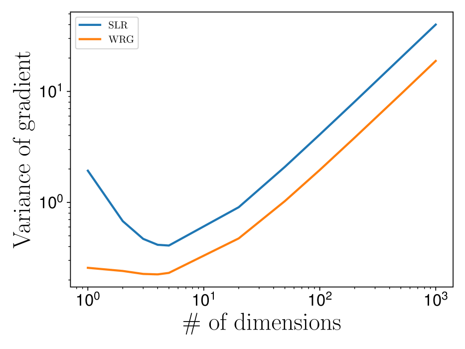
(a) Deterministic, ${\bf a}={\bf 1}$

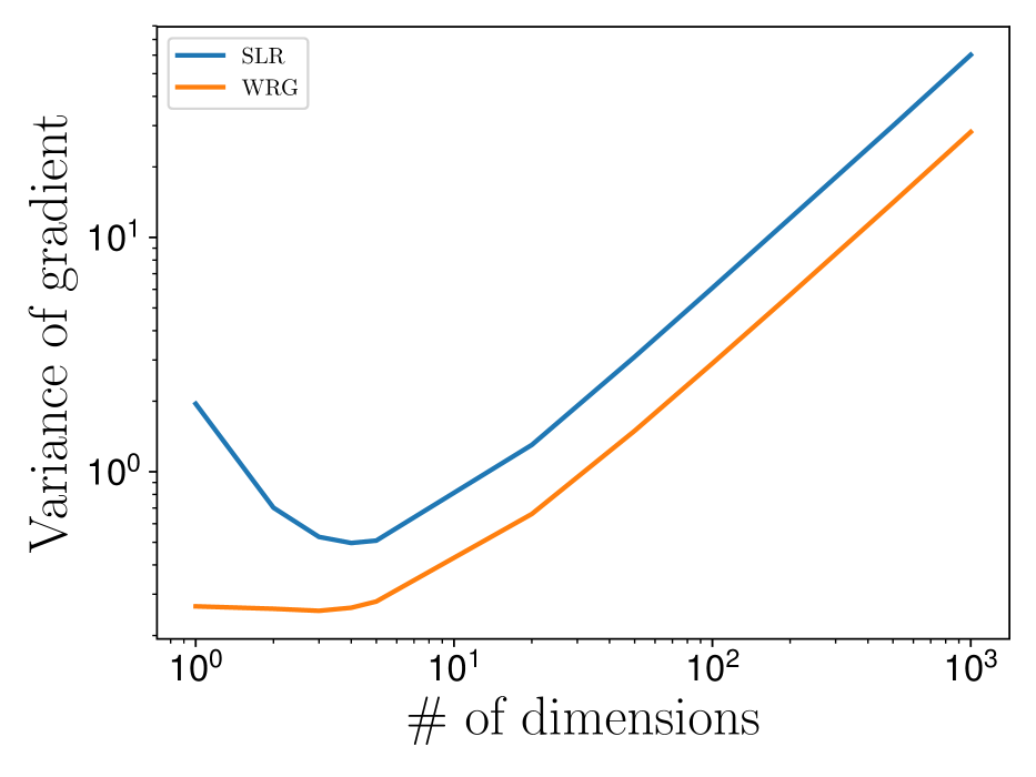
(b) Noisy, ${\bf a}={\bf 1}$

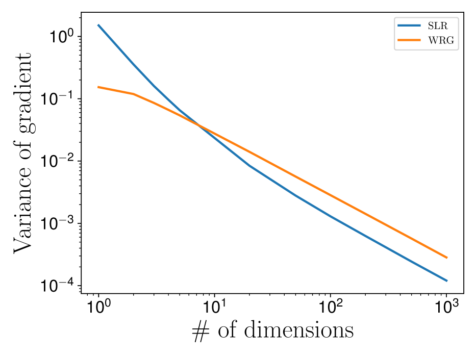
(c) Deterministic, ${\bf a}={\bf 0}$

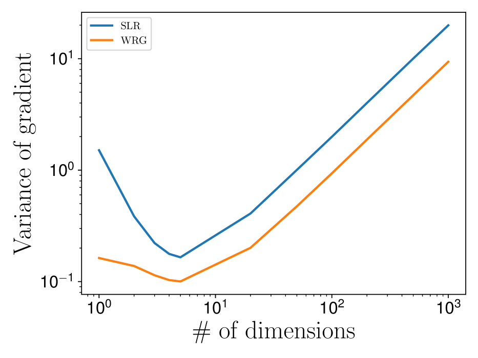
(d) Noisy, ${\bf a}={\bf 0}$

Figure 8: The confidence intervals correspond to one standard deviation of the estimate.

E.5 Multidimensional Gaussian Slice ratio gradient

In multiple dimensions the optimality equation in Eq. (5) is still valid, but the method to derive the normalized distribution and sampling method have to be modified. For simplicity, we consider the case of optimal sampling for the derivative w.r.t. $\mu$ for a spherical Gaussian. Motivated from the derivation for a single dimension, consider a method which would sample a unit vector on a sphere for a direction $\hat{{\bf r}}$, as well as a height $h$, then invert the distribution s.t. ${\bf x}=p^{-1}(h,\hat{{\bf r}})$, where $p^{-1}$ is a function s.t. $p\left({\bf x}\right)=h$ and ${\bf x}=r\hat{{\bf r}}$, i.e., it picks ${\bf x}$ in the direction $\hat{{\bf r}}$, which gives the desired probability density. The conversion from the $h$-coordinate to the ${\bf x}$-coordinate would still give the desired $\left|\frac{\textup{d}p\left({\bf x}\right)\hfill}{\textup{d}{\bf x}\hfill}\right|$ term; however, due to the change in the surface area as the radius $r$ is increased, there is an additional factor $r^{-(D-1)}$, where $D$ is the dimensionality. In other words, the sampling method has to be modified to cancel out this new factor, and the required distribution must have the property: $q({\bf x})\propto r^{D-1}\left|\frac{\textup{d}p\left({\bf x}\right)\hfill}{\textup{d}{\bf x}\hfill}\right|$. For a Gaussian base distribution we get $q({\bf x})\propto r^{D}\exp(-\frac{r^{2}}{2\sigma^{2}})$. The required distribution is the chi distribution:

$$q(z;k)=\frac{1}{2^{(k/2-1)}\Gamma(k/2)}z^{k-1}\exp(-\frac{z^{2}}{2})~{}~{}~{}\textup{where}~{}~{}~{}r=\sigma z~{}~{}~{}\textup{and}~{}~{}~{}k=D+1.$$ (48)

In fact, the Rayleigh distribution is a special case of this distribution for $D=1$, and the Maxwell-Boltzmann distribution is the case for $D=2$. Note that if one performs this sampling procedure, but while using $\tilde{D}=D-1$, then the sample comes exactly from the original Gaussian distribution $p\left({\bf x};\mu,\Sigma\right)$. This remark highlights that there are diminishing returns to changing the sampling distribution as the dimensionality of the space is increased, because the optimal sampling distribution tends to the original Gaussian distribution.

Derivation of the directional ratio gradient estimator (DRG):

The chi distribution $q(z;k)$ with k degrees of freedom is a distribution, s.t. $z$ is distributed according to the random variable $z=\sqrt{\sum_{i=1}^{k}x_{i}}$, where $x_{i}$ are distributed according to a Gaussian distribution with mean 0 and standard deviation 1. In other words, $z$ is distributed according to the length of the distance from the origin, when sampling from a spherical Gaussian with $k$ dimensions, and to sample from a Gaussian distribution, it suffices to sample a direction $\hat{{\bf r}}$ on the unit sphere, then sample the distance $z$ according to the chi distribution, and add a factor $\sigma z$ to correct for the scaling from the variance parameter. We can write the probability density of a Gaussian in spherical coordinates as

$$\mathcal{N}\left({\bf x};0,\sigma^{2}I\right)=\frac{1}{A}q(z;D),$$ (49)

where $A$ is the area of a D-dimensional hypersphere at radius $\sigma z$ given by $A=\frac{2\pi^{D/2}}{\Gamma\left(\frac{1}{2}D\right)}(\sigma z)^{D-1}$, and ${\bf x}=\sigma z\hat{{\bf r}}$, where $\hat{{\bf r}}$ is a vector sampled on the unit sphere. In cartesian coordinates, the gradient w.r.t. ${\bf x}$ can be written as

$$\frac{\textup{d}p\left({\bf x};0,\Sigma\right)\hfill}{\textup{d}{\bf x}\hfill}=\frac{1}{(2\pi)^{D/2}|\Sigma|^{1/2}}\exp\left(-{\bf x}^{T}\Sigma^{-1}{\bf x}\right)\times\left(-\Sigma^{-1}{\bf x}\right)=-\Sigma^{-1}{\bf x}p(x;0,\Sigma).$$ (50)

Translating this result to spherical coordinates, we have

$$\frac{\textup{d}p\left({\bf x};0,\Sigma\right)\hfill}{\textup{d}{\bf x}\hfill}=-\frac{z\hat{{\bf r}}}{\sigma}\frac{1}{A}q(z;D),$$ (51)

and

$$\left|\frac{\textup{d}p\left({\bf x};0,\Sigma\right)\hfill}{\textup{d}{\bf x}\hfill}\right|=\frac{z}{\sigma}\frac{1}{A}q(z;D).$$ (52)

If one applies the same directional sampling scheme, but instead of sampling from $q(z;D)$, one samples from a distribution proportional to $zq(z;D)$, one would be sampling from the desired distribution. By inspecting Eq. (48), it is clear that increasing the degrees of freedom by one adds the additional $z$ factor, so the optimal importance sampling distribution is

$$q({\bf x})=\frac{1}{A}q(z;D+1),$$ (53)

where ${\bf x}=\sigma z\hat{{\bf r}}$. To obtain the gradient estimator, divide $\frac{\textup{d}p\hfill}{\textup{d}\mu\hfill}=-\frac{\textup{d}p\hfill}{\textup{d}x\hfill}$ given in Eq. (51), with $q({\bf x})$ in Eq. (53):

$$\left.\frac{z\hat{{\bf r}}}{\sigma}\frac{1}{A}q(z;D)\middle/\frac{1}{A}q(z;D+1)\right.=\frac{\hat{{\bf r}}}{\sigma}\frac{zq(z;D)}{q(z;D+1)}=\frac{\hat{{\bf r}}}{\sigma}\frac{2^{1/2}\Gamma\left((D+1)/2\right)}{\Gamma\left(D/2\right)}$$ (54)

Derivation of the directional ratio gradient estimator while assuming a linear $\phi$ (DLRG):

The above derivation made our standard assumption that $\phi$ is ignored. Another option is to assume that $\phi$ varies linearly. The derivation is easily modified. From Eq. (52), we saw that it was necessary to sample from a distribution proportional to $zq(z)$. In the new derivation, it will be necessary to sample proportionally to $zq(z)\phi(z;D)$, which when $\phi$ is linear, is equivalent to sampling proportionally to $z^{2}q(z;D)$. Based on the same argument as in Eq. (53), the necessary sampling can be done by increasing the degrees of freedom by 2, i.e., one must sample from

$$q({\bf x})=\frac{1}{A}q(z;D+2).$$ (55)

Similarly to Eq. (54), the gradient estimator can be derived:

$$\left.\frac{z\hat{{\bf r}}}{\sigma}\frac{1}{A}q(z;D)\middle/\frac{1}{A}q(z;D+2)\right.=\frac{\hat{{\bf r}}}{\sigma}\frac{zq(z;D)}{q(z;D+2)}=\frac{2\hat{{\bf r}}}{z\sigma}\frac{\Gamma\left((D+2)/2\right)}{\Gamma\left(D/2\right)}=\frac{D\hat{{\bf r}}}{z\sigma},$$ (56)

where the last line follows from the property $\Gamma(n+1)=n\Gamma(n)$.

E.6 Sufficient conditions for an unbiased gradient estimator while ignoring importance weights from other dimensions

First we consider functions of the form $\phi({\bf x})=\sum_{i=1}^{D}\phi_{i}(x_{i})$, and show that ignoring the importance weights from dimension $j\neq i$ for the derivative w.r.t. $\theta_{i}$, still gives an unbiased gradient estimator. Note that $\mathbb{E}_{x_{i}\sim q(x_{i})}\left[\frac{p\left(x_{i}\right)}{q(x_{i})}\frac{\textup{d}\log p\left(x_{i};\theta_{i}\right)\hfill}{\textup{d}\theta_{i}\hfill}\mathbb{E}_{x_{j}\sim q(x_{j})}\left[\phi_{j}(x_{j})\right]\right]=\mathbb{E}_{x_{i}\sim p(x_{i})}\left[\frac{\textup{d}\log p\left(x_{i};\theta_{i}\right)\hfill}{\textup{d}\theta_{i}\hfill}\mathbb{E}_{x_{j}\sim q(x_{j})}\left[\phi_{j}(x_{j})\right]\right]=0$, because $\mathbb{E}_{x_{i}\sim p(x_{i})}\left[\frac{\textup{d}\log p\left(x_{i};\theta_{i}\right)\hfill}{\textup{d}\theta_{i}\hfill}Y\right]=\frac{\textup{d}\hfill}{\textup{d}\theta_{i}\hfill}\mathbb{E}\left[Y\right]=0$, for $Y$ statistically independent from $x_{i}$. This result means that if $\phi$ has a structure, such that different dimensions affect $\phi$ independently, then the gradient estimator will still be unbiased.

Next we show that even if the dimensions are not independent, in some cases the gradient estimator is unbiased. Notably, for a quadratic function $\phi({\bf x})={\bf a}^{T}{\bf x}+{\bf x}^{T}Q{\bf x}+c$, the gradient estimator will be unbiased. First note that the diagonal terms in the quadratic function are independent, so the gradient of that portion of the cost will be unbiased based on the previous example. Next consider the off-diagonal terms of ${\bf x}^{T}Q{\bf x}$, which are $x_{i}Q_{ij}x_{j}$. Note that the distributions we considered, namely the B, W, L and Beta distributions were all symmetric about the mean value $\mu_{j}$. Therefore $\mathbb{E}_{x_{j}\sim q(x_{j})}\left[Q_{ij}x_{j}\right]=\mathbb{E}_{x_{j}\sim p(x_{j})}\left[Q_{ij}x_{j}\right]$, and the derivative $\frac{\textup{d}\hfill}{\textup{d}\theta\hfill}\mathbb{E}_{x_{i}\sim p(x_{i})}\left[x_{i}\mathbb{E}_{x_{j}\sim q(x_{j})}\left[\frac{p(x_{j})}{q(x_{j})}Q_{ij}x_{j}\right]\right]$ remains unchanged even if one ignores the $p(x_{j})/q(x_{j})$ importance weights. This result implies that if the variance of the distribution $\sigma^{2}$ is small, such that $\phi$ is roughly quadratic in the range of the sampling distribution, then the gradient estimator will remain roughly unbiased.

Appendix F Additional justifications for approximations in the derivations

F.1 Ignoring importance weights in multidimensional slice ratio sampling

In Sec. 4 for the multidimensional case we considered factorized distributions $p\left({\bf x};\theta\right)=\prod_{i}p_{i}\left(x_{i};\theta_{i}\right)$, and for estimating the gradient w.r.t. $\theta_{i}$, we chose to ignore the importance weights from the other dimensions $j\neq i$. We justified the omission by noting that the unbiased gradient estimator would be given by

$$\frac{p_{\backslash i}\left({\bf x}_{\backslash i}\right)p_{i}\left(x_{i}\right)}{q_{\backslash i}({\bf x}_{\backslash i})q_{i}(x_{i})}\frac{\textup{d}\log p_{i}\left(x_{i}\right)\hfill}{\textup{d}\theta_{i}\hfill}\phi({\bf x}),$$ (57)

and that the variance would grow exponentially as the dimension increases, because of the growth of the variance of the $\frac{p_{\backslash i}\left({\bf x}_{\backslash i}\right)}{q_{\backslash i}({\bf x}_{\backslash i})}$ term. The assumption of factorized distributions may appear restrictive; however, note that this is the most common scenario in practice, and finding a solution in this setting is important. Moreover, note that by making the factorization assumption, we ended up with a worst case scenario, where as the dimension increases, the optimal unbiased importance sampling distribution will tend to the original distribution, thus showing that no gains are possible without adding in bias. Replacing the importance weights with their expected value is not just a convenience, but a necessity. If the distribution does not factorize, then such an omission may not be necessary, and good unbiased importance sampling distributions may exist, but our methods would not be directly applicable, and this is a topic for future work.

F.2 Omission of $\phi$ in optimality of slice ratio sampling derivation theoretical reasons

In the derivation of the slice ratio gradients, the optimization of the variance of $\frac{\textup{d}p\left(x;\theta\right)\hfill}{\textup{d}\theta\hfill}\phi(x)/q(x)$ was replaced with optimizing the variance of $\frac{\textup{d}p\left(x;\theta\right)\hfill}{\textup{d}\theta\hfill}/q(x)$. Here we explain the various reasons, which justify this omission, and show that in most realistic settings it is almost exactly the correct thing to do. We introduce three realistic settings to which this omission corresponds: 1. the estimation of $\phi$ is very noisy, 2. $\phi$ is high dimensional, 3. $\phi$ has high frequency variations at a length scale smaller than the range of the sampling distribution. In addition, note that another reasonable assumption might be to assume that $\phi(x)$ is linear, but the L-distribution (App. D) turns out to be optimal in this setting (in low dimensions).

$\phi$ is very noisy:

If $\phi$ is noise uncorrelated with $x$, then $\mathbb{V}\left[\frac{\textup{d}p\left(x;\theta\right)\hfill}{\textup{d}\theta\hfill}\phi(x)/q(x)\right]=\mathbb{V}\left[\frac{\textup{d}p\left(x;\theta\right)\hfill}{\textup{d}\theta\hfill}/q(x)\right]\mathbb{V}\left[\phi(x)\right]$, and one can ignore $\phi$ in the optimization. The same reasoning holds if $\phi(x)=\hat{\phi}(x)+\epsilon_{n}$, where $\epsilon_{n}$ is random noise with magnitude much larger than the variation of $\phi(x)$.

$\phi$ is high dimensional:

Consider the independent multidimensional sampling scenario justified in App. F.1, and estimating the variance of the gradient of one dimension $i$. The general gradient estimator is given by

$$\frac{\textup{d}\hfill}{\textup{d}\theta_{i}\hfill}\mathbb{E}_{{\bf x}\sim p\left({\bf x}\right)}\left[\phi({\bf x})\right]=\mathbb{E}_{{\bf x}\sim q({\bf x})}\left[\frac{p_{\backslash i}\left({\bf x}_{\backslash i}\right)p_{i}\left(x_{i}\right)}{q_{\backslash i}({\bf x}_{\backslash i})q_{i}(x_{i})}\frac{\textup{d}\log p_{i}\left(x_{i}\right)\hfill}{\textup{d}\theta_{i}\hfill}\phi({\bf x})\right],~{}~{}~{}~{}~{}~{}~{}\textup{where }p_{\backslash i}\textup{ is }\prod_{j\neq i}p_{j}\left(x_{j};\theta_{j}\right).$$ (58)

In the independent sampling case, we justified that $\frac{p_{\backslash i}\left({\bf x}_{\backslash i}\right)}{q_{\backslash i}({\bf x}_{\backslash i})}$ should be ignored if one hopes to make any gains in terms of variance reduction. We are left with estimating the variance of $\frac{p_{i}\left(x_{i}\right)}{q_{i}(x_{i})}\frac{\textup{d}\log p_{i}\left(x_{i}\right)\hfill}{\textup{d}\theta_{i}\hfill}\phi({\bf x})$. Note that $\phi({\bf x})$ still contains all dimensions other than $i$, i.e. $x_{j},$ where $j\neq i$ still matter; however, they are statistically independent of the gradient estimator, and thus the variation caused by $x_{j}$ acts as noise on the gradient signal. We call this, the sampling interference noise. If one assumes that the dimensionality is $D$, and that the variation of $\phi(x)$ is roughly the same in each dimension, then roughly a fraction $(D-1)/D$ of $\phi$ can be considered as noise for each gradient estimator. Thus, as the dimension increases, the variation in $\phi({\bf x})$ rapidly approaches equivalence to random noise, and rejecting the noise will be most important for reducing gradient variance.

$\phi$ has high frequency components:

Consider $\phi(x)=\hat{\phi}(x)+a\sin(\omega x)$. If $\omega$ is large compared to the sampling range, then $\sin(\omega x)$ is almost statistically independent to $x$, and can be viewed as noise. Such high frequency components occur when applying LR gradients to chaotic systems (Parmas et al.,, 2018), and correspond to the situation when LR vastly outperforms RP. Thus, reducing the variance of LR gradients in this scenario is important.

F.3 Additional experiments showing downsides of alternative approaches

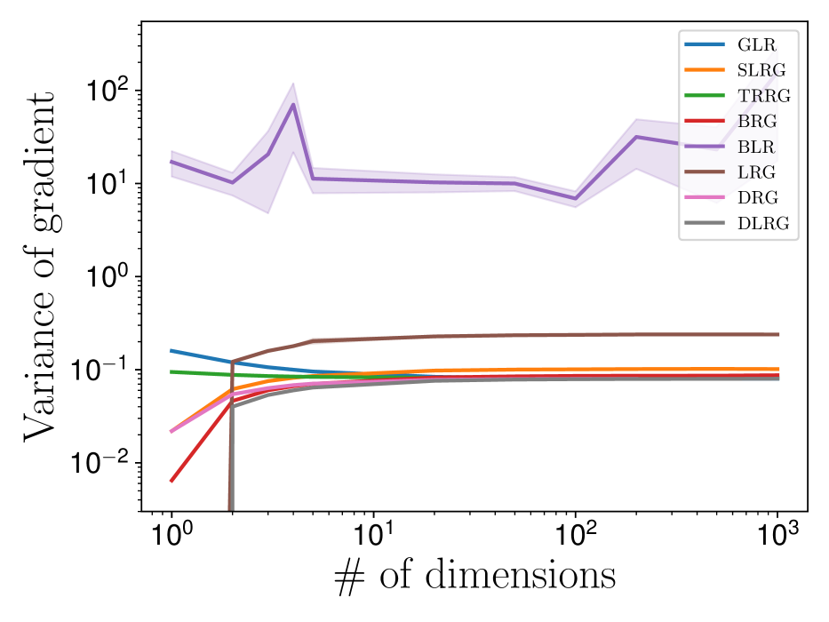
(a) Deterministic

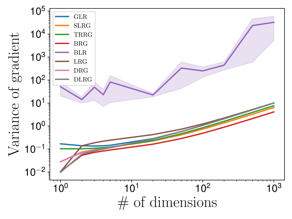
(b) Noisy

Figure 9: yadayada. The confidence intervals correspond to one standard deviation of the estimate.

In Fig. 9 we show experiments evaluating alternative optimal gradient estimators based on different assumptions, and explain that our approach in the main paper is better. We evaluated importance sampling based on the L-distribution (LRG), as well as the optimal importance sampling distribution in multiple dimensions without ignoring the importance weights from the other dimensions. DRG stands for directional ratio gradient, which omits $\phi$ in the derivation, but considers importance weights from all dimensions. DLRG assumes $\phi$ is roughly linear. The other results are the same as in the main section of the article: GLR—LR gradient with a Gaussian $p(x)$; SLRG—slice ratio gradient with a Gaussian $p(x)$; TRRG—truncated ratio gradient with $c=0.5$; BRG—slice ratio gradient with a Beta $p(x)$, and $\alpha=1.5$, plotted in Fig. 4(c); BLR—LR gradient with a Beta $p(x)$, and $\alpha=1.5$.

Results:

The alternative methods (LRG, DRG, DLRG) converge to GLR in the noisy setting for high dimensions, and show no gain in terms of variance reduction, whereas our proposed methods, SLRG and TRRG are able to show some advantage. In the deterministic case, at high dimensions LRG has higher variance than the other methods, because it has a larger sampling variance, which increases the sampling interference noise from the other dimensions, explained in Sec. F.2. A point which deserves discussion is that in the 1-dimensional deterministic case, LRG and DLRG show extremely low variance. The gradient estimator in this situation is given by $\frac{\textup{sgn}(x-\mu)}{\sigma\sqrt{-2\log(\epsilon_{h})+\epsilon_{x}^{2}}}\phi(x)=\frac{\textup{sgn}(x-\mu)}{x}\phi(x)$. Note that in the antithetic sampling setting, this estimator just becomes a finite difference $(\phi(x^{+})-\phi(x^{-}))/(2\Delta x)$, where the 2 comes from averaging two samples, and if $\phi$ is linear, then the gradient estimator would be exact with just one sampled pair (unlike the standard finite difference estimator, this estimator would be unbiased for non-linear $\phi$ as well). In the experiment, the curvature of $\phi$ was quite low, so LRG and DLRG gave extremely low variance in the 1-dimensional setting, but this advantage does not hold up, when the dimensionality is increased. In conclusion, the approximations we made are well justified.

Appendix G Truncated ratio gradient derivations

Recall that the truncated ratio gradient probability density function, sampling method and gradient estimator are given by the result below:

$$p_{tr}\left(x;c,\mu,\sigma\right) =\frac{\exp(-\frac{c^{2}}{2})}{1-\Phi(c)}\frac{1}{\sigma 2\sqrt{2\pi}}\frac{|x-\mu|}{\sqrt{(x-\mu)^{2}+\sigma^{2}c^{2}}}\exp(-\frac{(x-\mu)^{2}}{2\sigma^{2}})$$ (59)

$$~{}~{}~{}\textup{where}~{}\Phi(c)\textup{ is the cdf of a unit normal distribution},$$

$$x =\mu\pm\sigma\sqrt{\epsilon_{c}^{2}-c^{2}}~{}~{}~{}\textup{where}~{}~{}~{}\epsilon_{c}\sim\textup{truncG}(c,\infty)$$

$$~{}~{}~{}\textup{and}~{}\textup{truncG}(a,b)\textup{ is the unit normal truncated between }a\textup{ and }b,$$

$$\frac{\textup{d}\hfill}{\textup{d}\mu\hfill}\mathbb{E}_{x\sim p_{tr}\left(x\right)}\left[\phi(x)\right] =\mathbb{E}_{x\sim q(x)}\left[\textup{sgn}(x-\mu)\frac{2\epsilon_{c}}{\sigma}\frac{1-\Phi(c)}{\exp(-\frac{c^{2}}{2})}\phi(x)\right].$$

The pdf $p_{tr}\left(x;c,\mu,\sigma\right)$ satisfies the optimality Eq. (10), therefore, as long as it is a proper probability density, it is correct. We will show that the proposed sampling method corresponds to this pdf.

Without loss of generality, let $\mu=0$. The pdf of $\epsilon_{c}$ is given by

$$p\left(\epsilon_{c}\right)=\frac{1}{\sqrt{2\pi}}\exp\left(-\frac{\epsilon_{c}^{2}}{2}\right)\frac{1}{1-\Phi(c)},\textup{between }\epsilon_{c}\in[c,\infty].$$ (60)

Perform a change of coordinates from $\epsilon_{c}$ to $x$ and account for the stretching due to the Jacobian:

$$x=\sigma\sqrt{\epsilon_{c}^{2}-c^{2}}\Rightarrow\textup{d}x=\sigma\frac{\epsilon_{c}}{\sqrt{\epsilon_{c}^{2}-c^{2}}}\textup{d}\epsilon_{c},$$ (61)

note that $\sigma\epsilon_{c}=\sqrt{x^{2}+\sigma^{2}c^{2}}$, so

$$\frac{x/\sigma}{\sqrt{x^{2}+\sigma^{2}c^{2}}}\textup{d}x=\textup{d}\epsilon_{c},$$ (62)

therefore

$$p\left(\epsilon_{c}\right)\textup{d}\epsilon_{c} =\frac{1}{\sqrt{2\pi}}\exp\left(-\frac{\epsilon_{c}^{2}}{2}\right)\frac{1}{1-\Phi(c)}\frac{x/\sigma}{\sqrt{x^{2}+\sigma^{2}c^{2}}}\textup{d}x$$ (63)

$$=\frac{1}{\sqrt{2\pi}}\exp\left(-\frac{x^{2}}{2\sigma^{2}}+\frac{c^{2}}{2}\right)\frac{1}{1-\Phi(c)}\frac{x/\sigma}{\sqrt{x^{2}+\sigma^{2}c^{2}}}\textup{d}x$$

$$=\frac{\exp\left(-\frac{c^{2}}{2}\right)}{1-\Phi(c)}\frac{1}{\sigma\sqrt{2\pi}}\frac{x}{\sqrt{x^{2}+\sigma^{2}c^{2}}}\exp\left(-\frac{x^{2}}{2\sigma^{2}}\right)\textup{d}x.$$

This result is the desired probability distribution on the half-plane $[0,\infty]$. It is a normalized pdf by construction. Symmetrizing the distribution about 0, and shifting by a mean parameter $\mu$ gives the desired result. The gradient estimator is easily derived by $\nicefrac{{\frac{\textup{d}p\hfill}{\textup{d}\theta\hfill}}}{{q}}$.

Variance and gradient accuracy derivations:

The variance is most easily derived by working with the distribution on $\epsilon_{c}$ in Eq. (60). Note that if we symmetrize the distribution about 0, then the mean will be 0, and the variance can be estimated as the expectation of $x^{2}$ when sampling from half the distribution:

$$\mathbb{V}\left[x\right]=\int x^{2}p\left(\epsilon_{c}\right)\textup{d}\epsilon_{c}=\int\sigma^{2}(\epsilon_{c}^{2}-c^{2})p\left(\epsilon_{c}\right)\textup{d}\epsilon_{c}=\int\sigma^{2}\epsilon_{c}^{2}p\left(\epsilon_{c}\right)\textup{d}\epsilon_{c}-\sigma^{2}c^{2}.$$ (64)

So, we just need to find $\mathbb{E}\left[\epsilon_{c}^{2}\right]=\mathbb{V}\left[\epsilon_{c}\right]+\mathbb{E}\left[\epsilon_{c}\right]^{2}$. Denote $\mathcal{N}(x)$ is the unit variance Gaussian distribution, and $\Phi(x)$ is the cdf of the unit variance Gaussian, then the mean and variance of the 0 mean truncated Gaussian between $[c,\infty]$ can be written as $\mathbb{E}\left[\epsilon_{c}\right]=\frac{\mathcal{N}(c)}{1-\Phi(c)}$ and $\mathbb{V}\left[\epsilon_{c}\right]=1+\frac{c\mathcal{N}(c)}{1-\Phi(c)}-\left(\frac{\mathcal{N}(c)}{1-\Phi(c)}\right)^{2}$. Combining these two results:

$$\mathbb{E}\left[\epsilon_{c}^{2}\right]=1+\frac{c\mathcal{N}(c)}{1-\Phi(c)}.$$ (65)

Hence, the variance is

$$v(c)=\mathbb{V}\left[x\right]=\sigma^{2}\left(1+\frac{c\mathcal{N}(c;0,1)}{1-\Phi(c)}-c^{2}\right).$$ (66)

Next, we derive the variance of the gradient term $\frac{\textup{d}p\hfill}{\textup{d}\mu\hfill}/q$. Note that this term is given in Eq. (59) as $\textup{sgn}(x-\mu)\frac{2\epsilon_{c}}{\sigma}\frac{1-\Phi(c)}{\exp(-\frac{c^{2}}{2})}$, so the variance is

$$\mathbb{V}\left[\frac{\textup{d}p\hfill}{\textup{d}\mu\hfill}/q\right]=\mathbb{E}\left[\left(\frac{2\epsilon_{c}}{\sigma}\frac{1-\Phi(c)}{\exp(-\frac{c^{2}}{2})}\right)^{2}\right] =\mathbb{E}\left[\epsilon_{c}^{2}\right]\left(\frac{2}{\sigma}\frac{\left(1-\Phi(c)\right)}{\exp(-\frac{c^{2}}{2})}\right)^{2}$$ (67)

$$=\left(1+\frac{c\mathcal{N}(c;0,1)}{1-\Phi(c)}\right)\frac{4}{\sigma^{2}}\frac{\left(1-\Phi(c)\right)^{2}}{\exp(-c^{2})}.$$

Finally, note that the gradient accuracy $t(c)$ is defined as $1/\mathbb{V}\left[\frac{\textup{d}p\hfill}{\textup{d}\mu\hfill}/q\right]$.

Appendix H Evolution strategies in reinforcement learning

Evolution strategies are a technique based on sampling in the parameter space of a problem $p\left({\bf w};\theta\right)$, and applying LR gradients to optimize the objective $\mathbb{E}_{p\left({\bf w};\theta\right)}\left[\phi(w)\right]$. For example ${\bf w}$ may be the parameters of a neural network policy in reinforcement learning, and the objective is to find the distribution $p\left({\bf w};\theta\right)$ over the parameters ${\bf w}$, which gives the behavior with the largest expected reward. In this case, $\phi({\bf w})$ would be the return function for a particular parameter set ${\bf w}$. One would first sample parameters ${\bf w}$, these would be kept fixed for one episode of the agent’s behavior, the behavior would be evaluated based on a reward function, and the sum of the reward would be returned to the algorithm as $\phi({\bf w})$. LR gradients can be used to evaluate $\frac{\textup{d}\hfill}{\textup{d}\theta\hfill}\mathbb{E}_{{\bf w}\sim p\left({\bf w};\theta\right)}\left[\phi({\bf w})\right]$, and the objective can be optimized directly using gradient ascent. We implemented our new importance sampling schemes into David Ha’s Evolution Strategies code available from https://github.com/hardmaru/estool(Ha,, 2017) (note that our methods are not available from the link yet), and tested our methods on cart-pole swing-up and biped walker tasks illustrated in Fig. 10.

H.1 Experiments

In all experiments we used spherical Gaussian base distributions $p\left({\bf w};\theta\right)$ for the GLR, SLRG and TRRG methods, while the sampling distributions $q({\bf w})$ varied based on the importance sampling scheme. For BRG, we used a Beta base distribution, and applied the Beta slice ratio gradient method. We used antithetic sampling, i.e. we always sampled ${\bf w}$ in pairs, which are located opposite of each other in the distribution. If such a scheme is used, then any constant baseline $b$ (Greensmith et al.,, 2004), which is subtracted from the $\phi({\bf w})$ values will cancel out from the opposite pairs, and the effect of such baselines can be ignored. We did not use a weight decay. For TRRG, $c=0.5$, and for BRG, $\alpha=1.1$ in all cases. We used a CPU cluster for our experiments. Biped tasks were run on 33 cores, and cart-pole tasks were run on 5 cores. All tasks were run for 2000 policy improvement iterations (gradient steps), and repeated for several different random number seeds (details in tables). Because the samples from $q(x)$ do not correspond to the objective $\mathbb{E}_{p\left(x;\theta\right)}\left[\phi(x)\right]$, we separately evaluated the performance by sampling from $p\left(x;\theta\right)$ after every 10 iterations. Note that this was done only for evaluation purposes, and did not have any effect on the learning.

Cart-pole setup

State dimension: 5; Action dimension: 1; Policy: neural network with one hidden layer with 10 neurons and tanh activations, total number of parameters ${\bf w}$: 71; Optimizer: basic stochastic gradient ascent with one learning rate parameter; Number of samples per iteration: 32; Std $\sigma$ of Gaussian: 0.5. In addition to the standard cart-pole task, we considered a setting where we artificially add noise onto the $\phi({\bf w})$ values to simulate a setting where the rewards can only be observed stochastically, and test how our importance sampling methods cope with such noisy measurements. There are additional details in the table and figure captions.

Biped walker setup

State dimension: 24; Action dimension: 4; Policy: neural network with two hidden layers with 40 neurons each and tanh activations, total number of parameters ${\bf w}$: 2804; Optimizer: Adam with $\beta_{1}=0.99$ and $\beta_{2}=0.999$; Number of samples per iteration: 256; Std $\sigma$ of Gaussian: 0.04. We used reward normalization (Mania et al.,, 2018), which is a technique to ensure that scale of the rewards stays roughly constant by normalizing these with the standard deviation of the sampled returns $\phi$. This appeared to perform better for GLR than rank standardization as used in (Salimans et al.,, 2017).

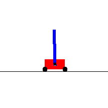
(a) Cart-pole swing-up

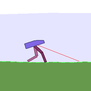
(b) Biped walker

Figure 10: Environments used in evolution strategies experiments.

Results

The results are in the tables and figures. The errorbars in the tables correspond to the sample standard deviation (so divide by the square root of the sample size to obtain a confidence interval), while the errorbars in the figures are already the standard deviation of the mean. The results act as a sanity check and show that our methods do work, while as expected the difference with standard GLR is small, because the improvement in accuracy is modest. On the other hand, the cart-pole swing-up experiments show that using the slice ratio gradient method allows the Beta base distribution to be competitive with Gaussian distributions. The experiments also show that SLRG can indeed have trouble with systems with a low stochasticty, e.g. the cart-pole. Moreover, the results confirm that our methods reduce gradient variance in stochastic settings. An important topic of future work will be finding distributions, which outperform Gaussians, and importance sampling techniques like our slice ratio gradient method will be crucial in such a pursuit.

Table 2: Cart-pole swing-up and balancing, no added noise, 32 samples per batch, SGD optimizer, average reward over whole training run, 10 experimental runs for each setting

Learn. rate	0.001	0.003	0.005	0.008	0.01
GLR	492.7 $\pm$ 15.6	694.4 $\pm$ 43.2	716.9 $\pm$ 77.4	792.6 $\pm$ 31.9	782.9 $\pm$ 43.1
SLRG	439.0 $\pm$ 12.2	580.3 $\pm$ 51.4	664.9 $\pm$ 55.2	763.2 $\pm$ 52.1	747.4 $\pm$ 72.7
TRRG	464.1 $\pm$ 5.6	676.6 $\pm$ 52.4	771.2 $\pm$ 31.7	809.5 $\pm$ 21.7	747.9 $\pm$ 102.1

Table 3: Cart-pole swing-up and balancing, no added noise, 32 samples per batch, SGD optimizer, average reward of last 100 parameter values, 10 experimental runs for each setting

Learn. rate	0.001	0.003	0.005	0.008	0.01
GLR	596.7 $\pm$ 39.7	881.2 $\pm$ 15.3	840.1 $\pm$ 103.2	904.4 $\pm$ 3.4	889.6 $\pm$ 47.4
SLRG	548.8 $\pm$ 7.6	723.1 $\pm$ 133.8	845.4 $\pm$ 82.0	887.0 $\pm$ 57.0	895.8 $\pm$ 24.7
TRRG	561.8 $\pm$ 16.0	867.1 $\pm$ 67.4	901.1 $\pm$ 3.5	905.8 $\pm$ 1.4	840.0 $\pm$ 136.0

Table 4: Cart-pole swing-up and balancing, 90 added noise standard deviation, 32 samples per batch, SGD optimizer, average reward over whole training run, the number of experimental runs for GLR, SLRG, TRRG were [10,10,50,50,10] for the learning rates from left to right respectively, and 20 runs for BRG in all cases.

Learn. rate	0.001	0.003	0.005	0.008	0.01
GLR	519.4 $\pm$ 36.9	668.1 $\pm$ 72.6	702.7 $\pm$ 66.3	690.3 $\pm$ 60.8	637.4 $\pm$ 42.8
SLRG	459.7 $\pm$ 10.4	608.5 $\pm$ 51.2	668.9 $\pm$ 70.8	710.5 $\pm$ 62.6	696.1 $\pm$ 64.9
TRRG	485.5 $\pm$ 8.0	658.0 $\pm$ 64.7	708.1 $\pm$ 64.8	699.2 $\pm$ 73.7	682.8 $\pm$ 71.4
BRG	409.1 $\pm$ 12.5	531.3 $\pm$ 16.4	600.8 $\pm$ 54.4	662.7 $\pm$ 70.6	723.0 $\pm$ 67.6

Table 5: Cart-pole swing-up and balancing, 90 added noise, 32 samples per batch, SGD optimizer, average reward of last 100 parameter values, the number of experimental runs for GLR, SLRG, TRRG were [10,10,50,50,10] for the learning rates from left to right respectively, and 20 runs for BRG in all cases.

Learn. rate	0.001	0.003	0.005	0.008	0.01
GLR	639.2 $\pm$ 81.6	807.6 $\pm$ 101.2	834.0 $\pm$ 82.8	810.2 $\pm$ 91.2	729.2 $\pm$ 103.8
SLRG	552.0 $\pm$ 5.9	771.0 $\pm$ 115.8	810.4 $\pm$ 108.9	845.1 $\pm$ 74.2	815.0 $\pm$ 83.3
TRRG	574.1 $\pm$ 21.4	818.1 $\pm$ 107.8	837.0 $\pm$ 86.0	814.0 $\pm$ 99.1	794.6 $\pm$ 121.0
BRG	535.8 $\pm$ 8.9	626.6 $\pm$ 69.9	736.8 $\pm$ 123.0	792.7 $\pm$ 115.0	873.5 $\pm$ 66.3

Table 6: Biped walker, 256 samples per batch, each parameter sample averaged over 4 episodes, Adam optimizer, reward scaled by standard deviation of rewards, average reward of whole training run, the number of experimental runs were [20,60,40,40,20] for the learning rates from left to right respectively

Learn. rate	0.005	0.01	0.015	0.02	0.04
GLR	14.6 $\pm$ 30.0	223.2 $\pm$ 62.1	264.2 $\pm$ 45.7	253.0 $\pm$ 51.6	260.9 $\pm$ 56.6
TRRG	31.6 $\pm$ 42.7	230.0 $\pm$ 39.5	250.2 $\pm$ 43.9	257.4 $\pm$ 46.0	251.2 $\pm$ 45.5

Table 7: Biped walker, 256 samples per batch, each parameter sample averaged over 4 episodes, Adam optimizer, reward scaled by standard deviation of rewards, average reward of last 100 parameter values, the number of experimental runs were [20,60,40,40,20] for the learning rates from left to right respectively

Learn. rate	0.005	0.01	0.015	0.02	0.04
GLR	38.4 $\pm$ 92.2	390.4 $\pm$ 61.5	376.6 $\pm$ 48.6	345.5 $\pm$ 63.4	347.9 $\pm$ 63.0
TRRG	104.1 $\pm$ 154.2	394.0 $\pm$ 34.1	363.3 $\pm$ 58.3	353.8 $\pm$ 62.3	352.5 $\pm$ 63.1

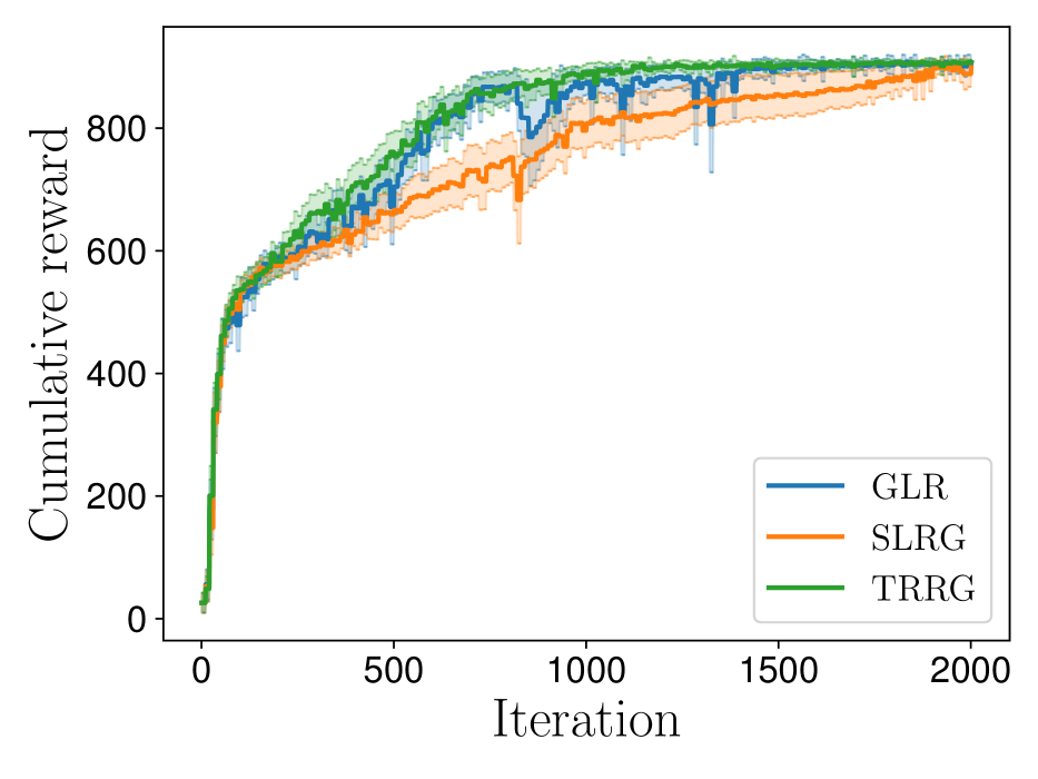
(a) Learning performance

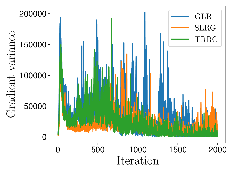
(b) Gradient variance

Figure 11: Cart-pole swingup, no noise, learning rate: 0.008 for all methods, errorbars show 1 standard deviation of the mean, TRRG’s $c=0.5$.

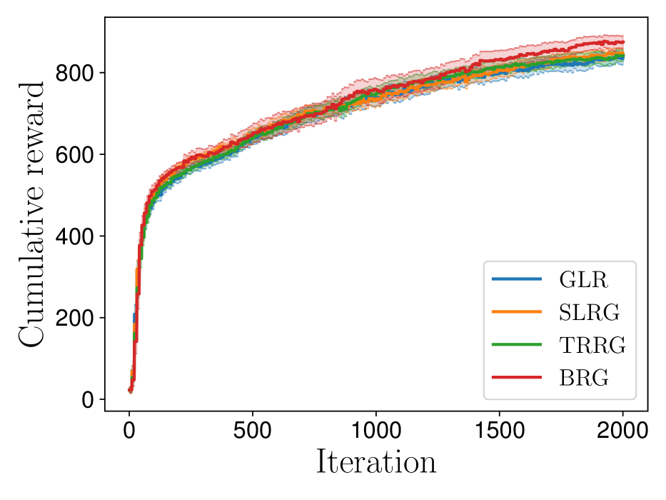
(a) Learning performance

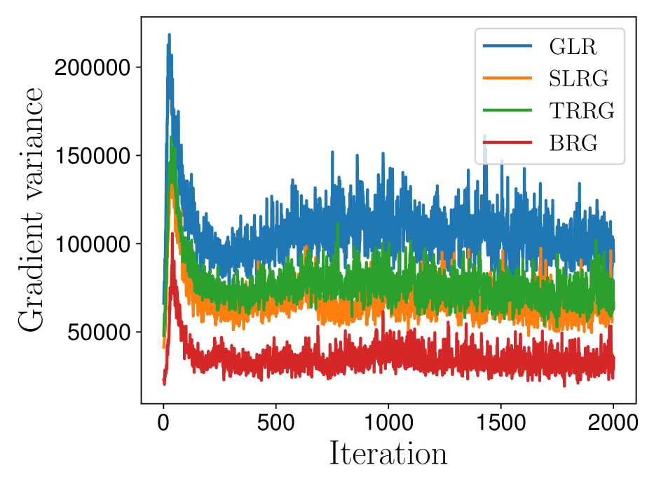
(b) Gradient variance

Figure 12: Cart-pole swingup; noise with std 90 added on cumulative reward; learning rates: GLR: 0.005, SLRG: 0.008, TRRG:0.005, BRG:0.01; errorbars show 1 standard deviation of the mean, BRG’s $\alpha=1.1$, TRRG’s $c=0.5$.

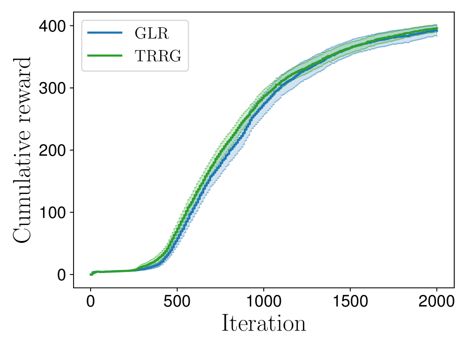
(a) Learning rate: 0.01

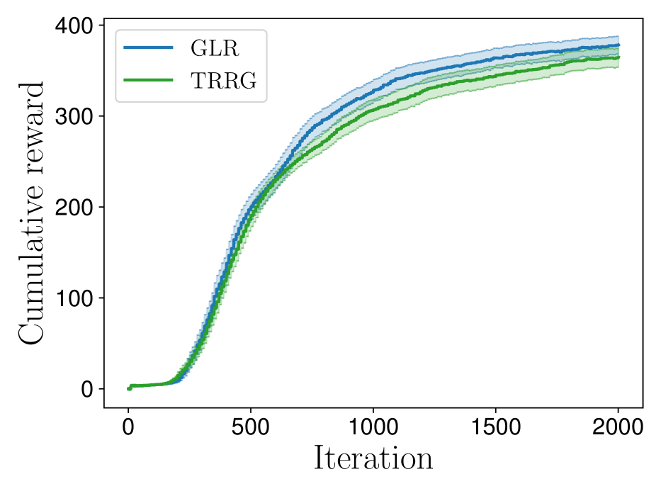
(b) Learning rate: 0.015

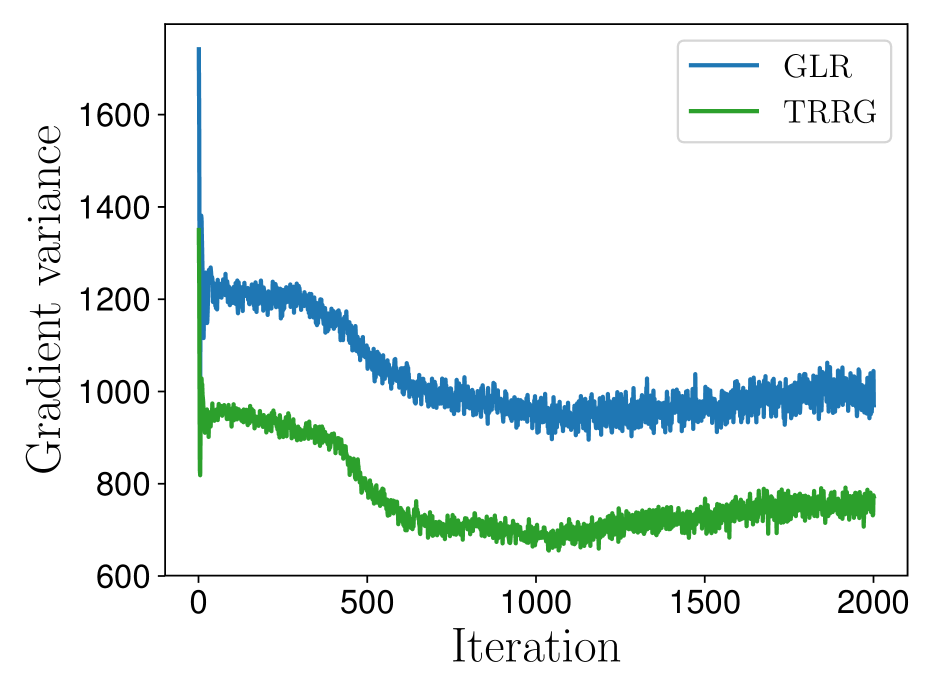
(c) Learning rate: 0.01

Figure 13: Biped walker; errorbars show 1 standard deviation of the mean, each parameter sample averaged over 4 episodes, TRRG’s $c=0.5$.

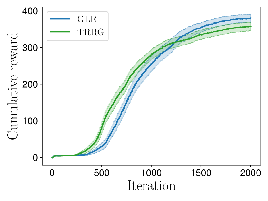
(a) Average results

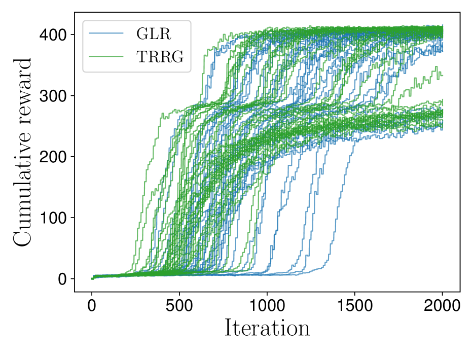
(b) Raw data

Figure 14: Biped walker; learning rate: 0.01, errorbars show 1 standard deviation of the mean, each parameter sample from 1 episode, 40 random number seeds, TRRG’s $c=0.5$; the final reward was bimodal, and while TRRG learned faster, more experiments converged to the lower local minimum.

References

- Asadi et al., (2017) Asadi, K., Allen, C., Roderick, M., Mohamed, A.-r., Konidaris, G., and Littman, M. (2017). Mean actor critic. stat, 1050:1.
- Chou et al., (2017) Chou, P.-W., Maturana, D., and Scherer, S. (2017). Improving stochastic policy gradients in continuous control with deep reinforcement learning using the beta distribution. In International Conference on Machine Learning, pages 834–843.
- Ciosek and Whiteson, (2018) Ciosek, K. and Whiteson, S. (2018). Expected policy gradients. In Thirty-Second AAAI Conference on Artificial Intelligence.
- Conti et al., (2018) Conti, E., Madhavan, V., Such, F. P., Lehman, J., Stanley, K., and Clune, J. (2018). Improving exploration in evolution strategies for deep reinforcement learning via a population of novelty-seeking agents. In Advances in Neural Information Processing Systems, pages 5027–5038.
- Corless et al., (1996) Corless, R. M., Gonnet, G. H., Hare, D. E., Jeffrey, D. J., and Knuth, D. E. (1996). On the Lambert W function. Advances in Computational mathematics, 5(1):329–359.
- Eisenach and Yang, (2019) Eisenach, C. and Yang, Z. (2019). Natural policy gradient for exponential families.
- Figurnov et al., (2018) Figurnov, M., Mohamed, S., and Mnih, A. (2018). Implicit reparameterization gradients. In Advances in Neural Information Processing Systems, pages 441–452.
- Fujita and Maeda, (2018) Fujita, Y. and Maeda, S.-i. (2018). Clipped action policy gradient. In International Conference on Machine Learning, pages 1592–1601.
- Gal, (2016) Gal, Y. (2016). Uncertainty in deep learning. PhD thesis, PhD thesis, University of Cambridge.
- Geffner and Domke, (2018) Geffner, T. and Domke, J. (2018). Using large ensembles of control variates for variational inference. In Advances in Neural Information Processing Systems, pages 9960–9970.
- Glynn, (1990) Glynn, P. W. (1990). Likelihood ratio gradient estimation for stochastic systems. Communications of the ACM, 33(10):75–84.
- Grathwohl et al., (2017) Grathwohl, W., Choi, D., Wu, Y., Roeder, G., and Duvenaud, D. (2017). Backpropagation through the void: Optimizing control variates for black-box gradient estimation. arXiv preprint arXiv:1711.00123.
- Greensmith et al., (2004) Greensmith, E., Bartlett, P. L., and Baxter, J. (2004). Variance reduction techniques for gradient estimates in reinforcement learning. Journal of Machine Learning Research, 5(Nov):1471–1530.
- Gu et al., (2015) Gu, S., Levine, S., Sutskever, I., and Mnih, A. (2015). MuProp: Unbiased backpropagation for stochastic neural networks. arXiv preprint arXiv:1511.05176.
- Gu et al., (2016) Gu, S., Lillicrap, T., Ghahramani, Z., Turner, R. E., and Levine, S. (2016). Q-prop: Sample-efficient policy gradient with an off-policy critic. arXiv preprint arXiv:1611.02247.
- Gu et al., (2017) Gu, S. S., Lillicrap, T., Turner, R. E., Ghahramani, Z., Schölkopf, B., and Levine, S. (2017). Interpolated policy gradient: Merging on-policy and off-policy gradient estimation for deep reinforcement learning. In Advances in Neural Information Processing Systems, pages 3846–3855.
- Ha, (2017) Ha, D. (2017). Evolving stable strategies. blog.otoro.net.
- Ha and Schmidhuber, (2018) Ha, D. and Schmidhuber, J. (2018). Recurrent world models facilitate policy evolution. In Advances in Neural Information Processing Systems, pages 2450–2462.
- Hoffman et al., (2013) Hoffman, M. D., Blei, D. M., Wang, C., and Paisley, J. (2013). Stochastic variational inference. The Journal of Machine Learning Research, 14(1):1303–1347.
- Jang et al., (2016) Jang, E., Gu, S., and Poole, B. (2016). Categorical reparameterization with Gumbel-Softmax. arXiv preprint arXiv:1611.01144.
- Jankowiak and Obermeyer, (2018) Jankowiak, M. and Obermeyer, F. (2018). Pathwise derivatives beyond the reparameterization trick. In International Conference on Machine Learning, pages 2240–2249.
- Jiang and Li, (2016) Jiang, N. and Li, L. (2016). Doubly robust off-policy value evaluation for reinforcement learning. In International Conference on Machine Learning, pages 652–661.
- Jie and Abbeel, (2010) Jie, T. and Abbeel, P. (2010). On a connection between importance sampling and the likelihood ratio policy gradient. In Advances in Neural Information Processing Systems, pages 1000–1008.
- (24) Jones, E., Oliphant, T., Peterson, P., et al. (2001–). SciPy: Open source scientific tools for Python. [Online; accessed May, 2019].
- Kingma and Welling, (2013) Kingma, D. P. and Welling, M. (2013). Auto-encoding variational Bayes. arXiv preprint arXiv:1312.6114.
- Maddison et al., (2016) Maddison, C. J., Mnih, A., and Teh, Y. W. (2016). The concrete distribution: A continuous relaxation of discrete random variables. arXiv preprint arXiv:1611.00712.
- Mania et al., (2018) Mania, H., Guy, A., and Recht, B. (2018). Simple random search of static linear policies is competitive for reinforcement learning. In Advances in Neural Information Processing Systems, pages 1800–1809.
- Mazoure et al., (2019) Mazoure, B., Doan, T., Durand, A., Hjelm, R. D., and Pineau, J. (2019). Leveraging exploration in off-policy algorithms via normalizing flows. arXiv preprint arXiv:1905.06893.
- Metz et al., (2019) Metz, L., Maheswaranathan, N., Nixon, J., Freeman, C. D., and Sohl-Dickstein, J. (2019). Understanding and correcting pathologies in the training of learned optimizers. In International Conference on Machine Learning.
- Mohamed et al., (2019) Mohamed, S., Rosca, M., Figurnov, M., and Mnih, A. (2019). Monte carlo gradient estimation in machine learning. arXiv preprint arXiv:1906.10652.
- Munos et al., (2016) Munos, R., Stepleton, T., Harutyunyan, A., and Bellemare, M. (2016). Safe and efficient off-policy reinforcement learning. In Advances in Neural Information Processing Systems, pages 1054–1062.
- Neal, (2003) Neal, R. M. (2003). Slice sampling. The annals of statistics, 31(3):705–767.
- Nesterov and Spokoiny, (2017) Nesterov, Y. and Spokoiny, V. (2017). Random gradient-free minimization of convex functions. Foundations of Computational Mathematics, 17(2):527–566.
- Owen, (2013) Owen, A. B. (2013). Monte Carlo theory, methods and examples.
- Parmas, (2018) Parmas, P. (2018). Total stochastic gradient algorithms and applications in reinforcement learning. In Advances in Neural Information Processing Systems, pages 10204–10214.
- Parmas et al., (2018) Parmas, P., Rasmussen, C. E., Peters, J., and Doya, K. (2018). PIPPS: Flexible model-based policy search robust to the curse of chaos. In International Conference on Machine Learning, pages 4062–4071.
- Peters and Schaal, (2008) Peters, J. and Schaal, S. (2008). Reinforcement learning of motor skills with policy gradients. Neural networks, 21(4):682–697.
- Rezende et al., (2014) Rezende, D. J., Mohamed, S., and Wierstra, D. (2014). Stochastic backpropagation and approximate inference in deep generative models. In International Conference on Machine Learning, pages 1278–1286.
- Ruiz et al., (2016) Ruiz, F., Titsias, M., and Blei, D. (2016). Overdispersed black-box variational inference. In 32nd Conference on Uncertainty in Artificial Intelligence 2016, UAI 2016, pages 647–656.
- Salimans et al., (2017) Salimans, T., Ho, J., Chen, X., Sidor, S., and Sutskever, I. (2017). Evolution strategies as a scalable alternative to reinforcement learning. arXiv preprint arXiv:1703.03864.
- (41) Schulman, J., Heess, N., Weber, T., and Abbeel, P. (2015a). Gradient estimation using stochastic computation graphs. In Advances in Neural Information Processing Systems, pages 3528–3536.
- (42) Schulman, J., Levine, S., Abbeel, P., Jordan, M., and Moritz, P. (2015b). Trust region policy optimization. In International Conference on Machine Learning, pages 1889–1897.
- Schulman et al., (2017) Schulman, J., Wolski, F., Dhariwal, P., Radford, A., and Klimov, O. (2017). Proximal policy optimization algorithms. arXiv preprint arXiv:1707.06347.
- Sutton and Barto, (1998) Sutton, R. S. and Barto, A. G. (1998). Reinforcement learning: An introduction, volume 1. MIT press Cambridge.
- Sutton et al., (2000) Sutton, R. S., McAllester, D. A., Singh, S. P., and Mansour, Y. (2000). Policy gradient methods for reinforcement learning with function approximation. In Advances in neural information processing systems, pages 1057–1063.
- Tang and Agrawal, (2018) Tang, Y. and Agrawal, S. (2018). Boosting trust region policy optimization by normalizing flows policy. arXiv preprint arXiv:1809.10326.
- Thomas and Brunskill, (2016) Thomas, P. and Brunskill, E. (2016). Data-efficient off-policy policy evaluation for reinforcement learning. In International Conference on Machine Learning, pages 2139–2148.
- Titsias and Lázaro-Gredilla, (2015) Titsias, M. K. and Lázaro-Gredilla, M. (2015). Local expectation gradients for black box variational inference. In Advances in neural information processing systems, pages 2638–2646.
- Tucker et al., (2018) Tucker, G., Bhupatiraju, S., Gu, S., Turner, R., Ghahramani, Z., and Levine, S. (2018). The mirage of action-dependent baselines in reinforcement learning. In International Conference on Machine Learning, pages 5022–5031.
- Tucker et al., (2017) Tucker, G., Mnih, A., Maddison, C. J., Lawson, J., and Sohl-Dickstein, J. (2017). REBAR: Low-variance, unbiased gradient estimates for discrete latent variable models. In Advances in Neural Information Processing Systems, pages 2627–2636.
- Walder et al., (2019) Walder, C. J., Nock, R., Ong, C. S., and Sugiyama, M. (2019). New tricks for estimating gradients of expectations. arXiv preprint arXiv:1901.11311.
- Weaver and Tao, (2001) Weaver, L. and Tao, N. (2001). The optimal reward baseline for gradient-based reinforcement learning. In Proceedings of the Seventeenth conference on Uncertainty in artificial intelligence, pages 538–545. Morgan Kaufmann Publishers Inc.
- Weber et al., (2019) Weber, T., Heess, N., Buesing, L., and Silver, D. (2019). Credit assignment techniques in stochastic computation graphs. In The 22nd International Conference on Artificial Intelligence and Statistics, pages 2650–2660.
- Wierstra et al., (2008) Wierstra, D., Schaul, T., Peters, J., and Schmidhuber, J. (2008). Natural evolution strategies. In 2008 IEEE Congress on Evolutionary Computation (IEEE World Congress on Computational Intelligence), pages 3381–3387. IEEE.
- Williams, (1992) Williams, R. J. (1992). Simple statistical gradient-following algorithms for connectionist reinforcement learning. Machine learning, 8(3-4):229–256.
- Xu et al., (2019) Xu, M., Quiroz, M., Kohn, R., and Sisson, S. A. (2019). Variance reduction properties of the reparameterization trick. In International Conference on Artificial Intelligence and Statistics.