Physics-Informed Deep Neural Network Method for Limited Observability State Estimation

Abstract

The precise knowledge regarding the state of the power grid is important in order to ensure optimal and reliable grid operation. Specifically, knowing the state of the distribution grid becomes increasingly important as more renewable energy sources are connected directly into the distribution network, increasing the fluctuations of the injected power.

In this paper, we consider the case when the distribution grid becomes partially observable, and the state estimation problem is under-determined. We present a new methodology that leverages a deep neural network (DNN) to estimate the grid state. The standard DNN training method is modified to explicitly incorporate the physical information of the grid topology and line/shunt admittance. We show that our method leads to a superior accuracy of the estimation when compared to the case when no physical information is provided. Finally, we compare the performance of our method to the standard state estimation approach, which is based on the weighted least squares with pseudo-measurements, and show that our method performs significantly better with respect to the estimation accuracy.

J. Ostrometzky and K. Berestizshevsky contributed equally to this work. This work was authored in part by the National Renewable Energy Laboratory (NREL), operated by Alliance for Sustainable Energy, LLC, for the U.S. Department of Energy (DOE) under Contract No. DE-AC36-08GO28308. The views expressed in the article do not necessarily represent the views of the DOE or the U.S. Government. The U.S. Government retains and the publisher, by accepting the article for publication, acknowledges that the U.S. Government retains a nonexclusive, paid-up, irrevocable, worldwide license to publish or reproduce the published form of this work, or allow others to do so, for U.S. Government purposes. This work was supported in part by the Laboratory Directed Research and Development (LDRD) Program at NREL, U.S. DOE OE as part of the DOE Grid Modernization Initiative, U.S. DOE Energy Efficiency and Renewable Energy Solar Energy Technologies Office, DARPA RADICS under Contract FA-8750- 16-C-0054, and DTRA grant HDTRA1-13-1-0021.

I Introduction

The problem of state estimation (SE) in power grids involves the estimation of a part of the variables of the power-flow equations (PFE), based on noisy measurements of the available variables. The SE is an essential inference tool that enables advanced control and automation capabilities for the grid operator. Examples of these capabilities are the Volt/Var control during a normal operation and feeder reconfiguration during restoration from an emergency. In the fully observable case, namely, when the number of unknown variables is smaller than the number of the available measurements, the weighted least squares (WLS) method [1] is well developed and widely used by the utilities. In this paper, we focus on the under-determined case, namely when the number of the unknowns is larger than the number of measurements. This is a typical case in distribution networks, where the measurement infrastructure is insufficient [2], as well as in grids under failures/attacks.

Figure 1: A high level illustration of the proposed DNN-based distributed system state estimation. The estimation process infers the voltages phasors $\underline{\hat{v}}(t)$ at the partially observable (PO) time step $t$, based on the previous $T-1$ fully observable time steps. All the measurements at time-step $t$ are used during training as the ground truth (GT). The red parts depict the training procedure which enforces the power flow equations feasibility.

The challenge of identifying a critical failure/attack and recovering the network state was the subject of many studies, with a major focus on transmission systems [3, 4, 5]. As for the distribution system state estimation (DSSE) problem, it becomes increasingly important due to the extensive penetration of highly-fluctuating power-injection sources such as renewable energy sources (e.g., photo-voltaic panels [6]). Thus, DSSE has been studied extensively in the recent literature; for review of the state-of-the-art methods, see, e.g., [7, 8] and references therein. Sensor placement strategies have been devised to derive additional measurements required for full observability [9, 10, 11]. Machine learning (ML) and signal processing tools have been used to derive pseudo-measurements using existing sensors and/or historical data [12, 13, 14], and to use them for further estimation purposes. However, installing sensors might be prohibitively costly, whereas off-the-shelf ML methods require large amounts of data to obtain a good estimation accuracy. Finally, several recent works attempt to directly address the under-determined estimation problem by leveraging the low-rank structure of the measurements [15, 16, 17, 18]. These approaches can be viewed as regularized WLS methods, wherein the regularization term is aimed at minimizing the rank of the data matrix.

In this paper, we consider the DSSE problem, in which the grid is observable during normal operation, and becomes unobservable unexpectedly due to, e.g., cyber attacks or physical failures. A high-level diagram of our methodology is depicted in Fig. 1. Our methodology leverages a deep neural network (DNN) to estimate the grid state based on historical data. Unlike standard DNN training methods, here, we modify the training to explicitly incorporate the physical information of the grid topology based on the line/shunt admittance. This is achieved by using the AC PFE as a loss function regularizer during the training of the DNN. This modification allows to reduce the size of the DNN solution search space, which in turn contributes to a better convergence during the training of the model, and leads to a higher estimation accuracy compared to the standard (non-regularized) methods.

Our approach can be viewed as a physics-informed ML approach that leverages the physical structure of the problem to improve the performance of a standard ML algorithm. In this respect, our work is closely related to [19], where the authors proposed to use the approximate separability property of the DSSE, and designed a pruned DNN via placement of phasor measurements units (PMUs) at key points in the grid. Our approach, on the other hand, optimizes the SE task by exploiting the known admittance matrix information, without specific PMU placement requirements, and can be applied to the existing grid infrastructure. The main contribution of our paper is an improved DSSE methodology under limited observability, combining a DNN with a physics-informed regularization.

To demonstrate the proposed method, we employ an experimental setup based on the IEEE 37-Node test feeder [20] with real-world generation and load data. We show the performance of our method on a number of partially-observable scenarios, achieving a consistently more accurate estimations, when compared to: (i) DNN-based approaches that do not use the PFE information; and (ii) the standard WLS method, based upon basic pseudo-measurements (which replaces the unobservable power phasors).

The rest of this paper is organized as follows: In Section II we present the definitions, the theory, and the development of our approach. Section III describes the experiments and the analysis of the resulting estimates. Lastly, Section IV concludes this paper and discusses future research challenges.

Nomenclature

Term	Domain	Description
$T$	$\mathbb{N}$	Num. of observation time steps
$N$	$\mathbb{N}$	Num. of nodes in the grid
$N_{s}(t)$	$\mathbb{N}$	Num. of observable power phasors
$N_{v}(t)$	$\mathbb{N}$	Num. of observable voltage phasors
$Y$	$\mathbb{C}^{N\times N}$	Admittance matrix
$\underline{s}(t)$	$\mathbb{C}^{N}$	Vector of complex power phasors
$\underline{v}(t)$	$\mathbb{C}^{N}$	Vector of complex voltage phasors
$\mathcal{O}^{t}$	$\mathbb{R}$	Degree of observability; $;\in[0,1]$
$\lambda$	$\mathbb{R}$	Regularization coefficient; $\in[0,\infty)$

II Theory and Methodology

In order to present our methodology, we first need to define the environment of interest, and to formulate the problem.

II-A Physical Environmental Assumptions

We assume a known grid topology and sensing capabilities, detailed as follows:

1. The distribution grid topology is fixed and the admittance matrix, $Y$, is considered known.

2. Each bus in the grid can report at each time step one of the following types of measurements: (i) none, (ii) power phasor, and (iii) power and voltage phasors.

3. During normal operation the grid is fully observable, that is both the power and voltage phasors are reported from all the buses at regular times. Prior to a partially observable time step, the estimator has guaranteed access to $T-1$ fully observable time steps.

4. For brevity, we focus on a single-phase estimation, basing our development on the single-phase AC PFE. The extension to multi-phase networks is straightforward, by leveraging multi-phase PFE as in, e.g., [21].

II-B Power System Model and Observability

We consider a distribution network consisting of one slack bus and $N-1$ PQ-buses. The PFE are given by

$$\underline{s}(t)=\mathsf{diag}(\underline{v}(t))Y^{*}\underline{v}^{*}(t)$$ (1)

where $\underline{s}(t)\in\mathbb{C}^{N};\underline{v}(t)\in\mathbb{C}^{N}$ are complex vectors that collect the apparent power injections and voltage phasors at time index $t$, respectively.

We assume that each bus can report at a given time step, $t$, one of the following combinations of measurements: $\{\emptyset;s(t);\{s(t),v(t)\}\}$, where $s(t)$ is the apparent power injection, and $v(t)$ is the phasor of the complex bus voltage. $\emptyset$ represents the empty set, meaning, that no measurement is being reported at time step $t$ by the bus. Let $N_{s}(t)$ and $N_{v}(t)$ denote the number of the observable power phasors and voltage phasors, respectively, at time step $t$.

For any $N_{s}(t)\in\{0,\ldots,N\}$; $N_{v}(t)\in\{0,\ldots,N\}$, let

$$\left.\mathcal{O}(N_{s}(t),N_{v}(t))\triangleq\frac{N_{s}(t)+N_{v}(t)}{2N}\right.$$ (2)

denote the degree of observability of the system. We also use the shorthand notation $\mathcal{O}^{t}:=\mathcal{O}(N_{s}(t),N_{v}(t))$ to denote the degree of observability at time $t$. Note that $\mathcal{O}^{t}=1$ represents an over-determined system (at time step $t$), whereas $\mathcal{O}^{t}=0$ represents the zero-observability case (in which all buses report $\emptyset$). Also, observe that $\mathcal{O}^{t}\geq 0.5$ is a necessary condition for solvability of (1) at time $t$.

II-C Problem Formulation

This section defines the specification of the DSSE problem according to the assumptions described in Section II-A. Let us denote by a Sudden-Failure-State-Estimator (SFSE) an estimator that respects the following specification:

SFSE($T,t,N_{s}(t),N_{v}(t)$)

Inputs:

full history before time $t$: $\text{ }\{\underline{s}(\tau),\underline{v}(\tau)\}_{\tau=t-1-T}^{t-1}$
partial measurements set at time $t$:        
$[s_{1}(t),\ldots,s_{N_{s}(t)}(t)];[v_{1}(t),\ldots,v_{N_{v}(t)}(t)]$.

Output:

$\emph{ voltage estimation at time $t$:}\text{ }\underline{\hat{v}}(t)$.

Here $T$ is a design parameter that denotes the guaranteed number of time steps that are fully observable ($N_{s}(\tau)=N_{v}(\tau)=N$, and therefore $\mathcal{O}^{\tau}=1;\tau=t-1-T,\ldots,t-1$), prior to the time of the failure $t$, at which $\mathcal{O}^{t}<0.5$. In other words, given a fully observable history of $T-1$ time steps, the goal is to complete the non-observable portion of the measurements in the last time step.

II-D DNN-Based SFSE Solution

We propose a neural-network model to solve the SFSE($T,t,N_{s}(t),N_{v}(t)$) problem (as formulated in Section II-C). This model is depicted as a block diagram in Fig. 2, and consists of two main components: feature extractor and regressor.

Figure 2: DNN model for the DSSE problem under the SFSE specifications.

The feature extractor receives as an input the standardized phasor data of the fully observable period $[t-T-1,t-1]$, and of the partially observable time step $t$. The phasors are assumed to be in a rectangular representation, but to simplify the architecture and the back-propagation process, we avoid using complex numbers in the neural network. Thus, each complex input term is treated as two real numbers (based on the real and imaginary parts of the original complex term). In essence, each observable time step is represented by a $4N$-dimensional vector containing $N$ pairs that represent the power phasors ($\underline{s}(\tau)$) and $N$ pairs that represent the voltage phasors ($\underline{v}(\tau)$). The feature extractor employs Long-Short-Term-Memory (LSTM) [22] module to extract temporal features $\underline{h}_{fo}\in\mathbb{R}^{\lceil{}\frac{N}{3}\rceil{}}$ from the fully observable time series. In addition, a fully connected neural network computes the features $\underline{h}_{po}\in\mathbb{R}^{\lceil{}\frac{N}{6}\rceil{}}$ from the partially observable time step. The $\underline{h}_{fo}$ and the $\underline{h}_{po}$ features are finally concatenated to form a unified feature vector $\underline{h}\in\mathbb{R}^{\lceil{}\frac{N}{2}\rceil{}}$. The sizes of the feature vectors were found empirically based on a smaller data set.

The regressor component of the model infers from the feature vector $\underline{h}$ the full voltage phasor vector, $\underline{\hat{v}}(t)$, represented by a $2N$ dimensional real-valued vector, where each pair of values corresponds to a voltage phasor in a rectangular form. The regressor module employs fully connected neural networks to find the non-scaled estimate of the voltage phasors and to determine the coefficients $\underline{w},\underline{b}\in\mathbb{R}^{2N}$. These coefficients scale and shift the non-scaled estimates to obtain the final voltage estimation, $\underline{\hat{v}}(t)$.

In the proposed DNN (depicted in Fig. 2) all the fully connected networks [23] use hyperbolic tangent activation functions to allow both positive and negative ranges. In the feature extractor, the fully connected network is of the shape $2(N_{s}+N_{v})\rightarrow 2(N_{s}+N_{v})\rightarrow N/6$. The LSTM module is composed of two stacked LSTM, where the first takes sequence of $4N$ long vectors and produces a sequence of vectors of size $2N$ which are fed to the second LSTM that produces a single output vector of a size $N/3$. In the regressor, the top fully connected network is in fact two fully connected sub-networks in parallel, each taking a vector of a size $\frac{N}{2}$ and producing a $2N$-sized vector. The bottom fully connected network is of the shape $\frac{N}{2}\rightarrow\frac{N}{2}\rightarrow\frac{N}{2}\rightarrow\frac{N}{2}\rightarrow\frac{N}{2}\rightarrow 2N$.

II-E Physics-Informed Loss Function

To design a physics-informed training algorithm, we introduce a regularization term into the DNN loss function $\mathcal{L}$, formalized as follows:

$$\mathcal{L}(\underline{s},\underline{v},\underline{\hat{v}},Y,\lambda)=||\underline{v}-\underline{\hat{v}}||^{2}+{\lambda}||\underline{s}-\mathsf{diag}(\underline{\hat{v}})Y^{*}\underline{\hat{v}}^{*}||^{2}$$ (3)

where the vectors $\underline{s}(t),\underline{v}(t)\in\mathbb{C}^{N}$ contain the entries of the measured complex power and voltage variables, respectively; the vector $\underline{\hat{v}}(t)\in\mathbb{C}^{N}$ contains the DNN estimated output of the complex voltage; and $\lambda\in\mathbb{R}$ is a weighting coefficient. The $||\underline{z}||$ operation over the complex vector $\underline{z}\in\mathbb{C}^{N}$ is defined by $\sum_{i=1}^{N}|z_{i}|^{2}$. Note that the vector $\underline{s}(t)$ contains all $N$ power phasors, whereas only $N_{s}(t)$ elements are introduced to the DNN as an input.

In essence, (3) expresses a loss function comprised of two terms. The first term is a standard squared-error expression, whereas the second term penalizes non-feasible PFE solutions. The hyperparameter $\lambda$ is used to set the ratio between the two terms.

II-F Weighted Least Squares Baseline

This section describes the WLS-based solution of the SFSE problem as stated in section II-C. At the time of the failure, $t$, we assume an input consisting of previous $T-1$ fully observable time steps, containing $N$ power phasors and $N$ voltage phasors. At time $t$, only $N_{s}(t)$ power phasors and $N_{v}(t)$ voltage phasors are available. We mostly focus on the case where $N_{v}(t)=0$ (all the voltages phasors are unobservable) and we perform several experiments using different $N_{s}(t)$ values. The WLS method will be used as a baseline for comparison against our DNN-based approach.

As a preliminary stage, the missing $N-N_{s}(t)$ power phasors are completed by duplicating their last known values (from time step $t-1$). The weights for the WLS optimization are intended to re-weight the PFE residuals. These weights are computed as follows:

$$W_{i}\triangleq 1/\text{std}\Big{(}\{s_{i}(\tau)\}_{\tau=t-1}^{t-1-T}\Big{)}$$ (4)

for $1\leq i\leq N$, where $\text{std}(\{s_{i}(\tau)\})$ is the standard deviation of the complex sequence $\{s_{i}(\tau)\}$, given by the sum of the standard deviation of the real parts and the imaginary parts of the sequence. The essence of this re-weighting is to give higher weights to measurements which are less likely to fluctuate (i.e., have a lower temporal variance).

The optimization variables are the voltage phasors ($\underline{\hat{v}}(t)=[\hat{v}_{1}(t),\ldots,\hat{v}_{N}(t)]$) in a rectangular representation. The initial guesses for the terms of $\underline{\hat{v}}(t)$ are set to $\underline{v}(t-1)$.

With $N_{s}(t)$ observable powers and $N-N_{s}(t)$ speculatively completed power phasors gathered in a vector $\hat{s}(t)$ and with the admittance matrix $Y$ fully known, the WLS optimizer solves the following minimization problem²:

$$\min_{\underline{\hat{v}}}F(\underline{\hat{v}}):=\frac{1}{2}\sum_{i=1}^{N}W_{i}(\Re\{f_{Y,\underline{\hat{s}}}(\underline{\hat{v}},i)\}^{2}+\Im\{f_{Y,\underline{\hat{s}}}(\underline{\hat{v}},i)\}^{2})$$ (5)

where the function $f_{Y,\underline{\hat{s}}(t)}(\underline{\hat{v}}(t),i):\mathbb{C}^{N}\rightarrow\mathbb{C}$ is the residual function obtained from the difference between the left-hand-side and the right-hand-side of the $i$th PFE with respect to the admittance matrix $Y\in\mathbb{C}^{N\times N}$ and the power and voltage complex vectors $\underline{\hat{s}}(t),\underline{v}(t)\in\mathbb{C}^{N}$. Namely²:

$$f_{Y,\underline{\hat{s}}}(\underline{\hat{v}},i)\triangleq\hat{s}_{i}-\sum_{j=1}^{N}\hat{v}_{i}\cdot Y_{i,j}\cdot\hat{v}_{j}^{*}$$ (6)

The optimization procedure for this problem followed the Levenberg-Marquardt method using the implementation available via the scipy Python module.

III Experimental Demonstration

In order to demonstrate our methodology, we designed a dedicated experimental setup, based on real-world data.

III-A Experimental Design and Data Preparation

Our experimental setup is based on a real-world distribution-grid load data collected from feeders in Anatolia, CA during the week of August 2012 [24]. The data includes the active power consumed (i.e., the active load) of eight houses, sampled continuously at a 1-second resolution for a full week (overall, $604800$ samples per house). In addition, the generation power from a PV panel-array that was connected to the same feeder was also recorded (at the same time indexes).

Using these measurements, we implemented a test-case scenario, based on a modified single-phase IEEE 37-node test feeder as follows:

1. For each of the eight reported active power time series, a random power-factor value was generated (between 0.96 and 0.98), and used to calculate a corresponding time series of the reactive power components, establishing eight complex power phasors, $s_{i}(t);i\in{[1,\ldots,8]}$;

2. 25 of the buses of the test case were assigned with one of the eight available power-phasors, $s_{i}(t)$. Thus, the eight power-phasors were duplicated (in a circular manner) and incorporated randomly to 25 of the buses;

3. Similarly, a power phasor was created from the available PV-panel generated power measurements, $s_{pv}(t)$, and was duplicated and randomly assigned onto 18 buses;

4. In case of buses that were assigned both a load power phasor, $s_{i}(t)$, and the generation power phasor, $s_{pv}(t)$, the two phasors were summed.

An illustration of the test case, including the nodes which were chosen as loads and as generators (based on available measured time series), is depicted in Fig. 3. The admittance matrix, $Y$, of the same test case is depicted in Fig. 4.

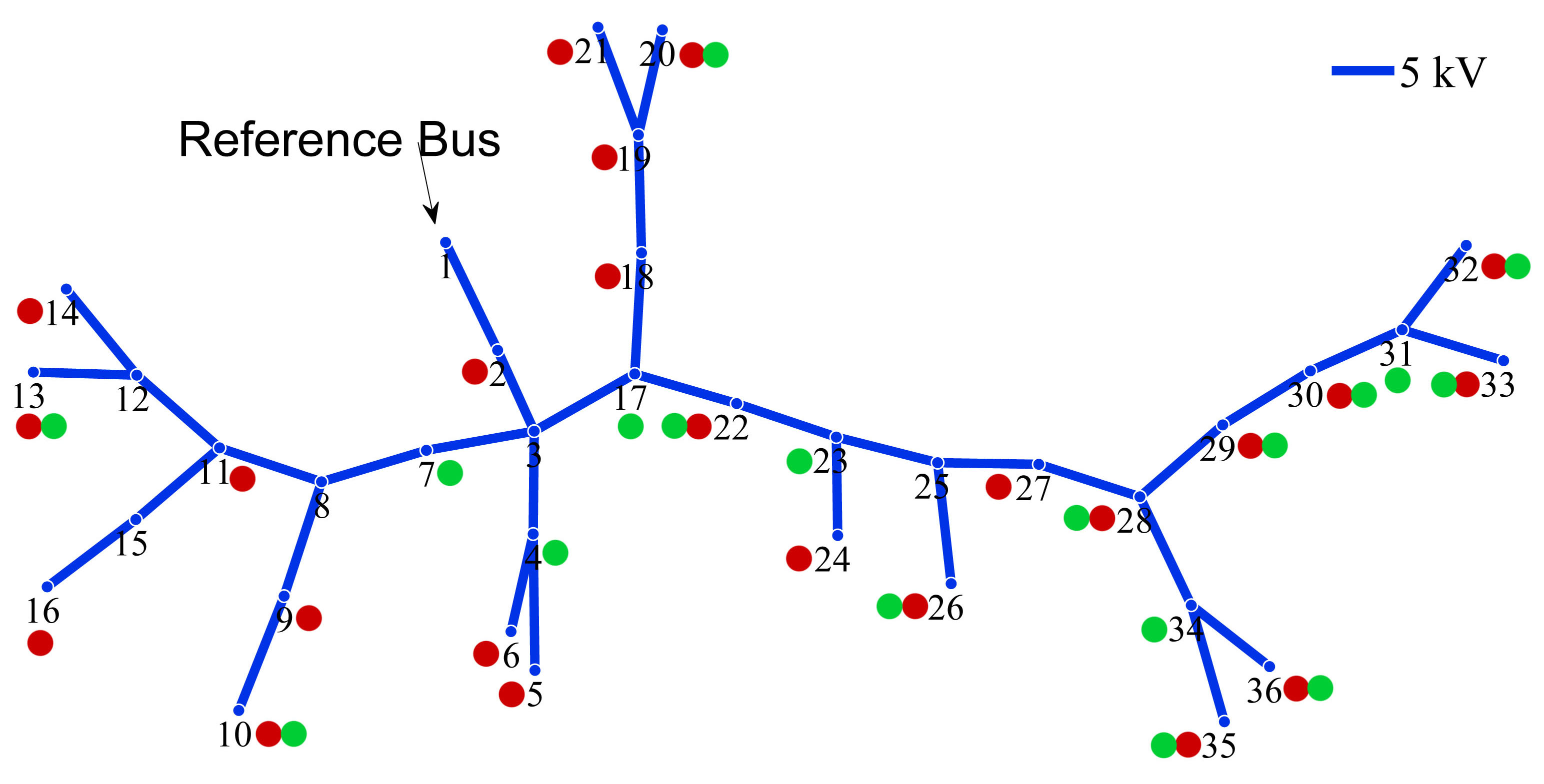
Figure 3: The topology of IEEE-37 Node test feeder distribution grid, consisting of 1 substation (also referred to as a reference bus) and 35 additional regular buses. The graph edges stand for 5kV branches. The reference bus is marked, as well as all the nodes that were assigned as loads (in red) and as generators (in green).

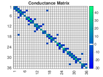
(a) Re{Y}

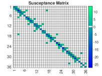
(b) Im{Y}

Figure 4: The Admittance Matrix, $Y$, for the IEEE 37-Node test feeder distribution grid, divided into the real part (a) , and the imaginary part (b) (both measured in Mega-Siemens).

After acquiring all the time series (i.e., the phasor vectors $\underline{s}(t)$ with measurements for each of the buses in the test case), we smoothed the data using a 60-sample moving average window, and then downsampled the time series by a factor 60. In other words, we smoothed the data using a low-pass-filter (a moving average over 60 values, sampled at $1$ Hz), and then took one sample per minute. By doing so, we: 1) Reduced the granularity of the data from 1-second to 1-minute, which reduces the complexity of the estimation workflows; 2) By smoothing the data prior to the downsampling operation, we minimized the chance of possible aliasing, and at the same time dampened the measurement- and other additive-noise by a factor of 60 [25]. As a result, the time series length was reduced to 10080 time steps. Using the smoothed and downsampled power-phasors time series, we utilized Matpower [26] power-flow solver to generate the corresponding phasors $\underline{s}(t)$ and $\underline{v}(t)$ for all the time steps available. The Matpower calculation was done based on a given and known admittance matrix, $Y$, using the full AC-model PFE. The Matpower output phasors are plotted in Fig. 5.

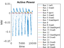
(a) Pd buses 1-18

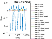
(b) Qd buses 1-18

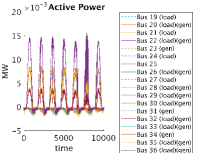
(c) Pd buses 19-36

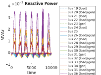
(d) Qd buses 19-36

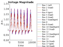
(e) Vm buses 1-18

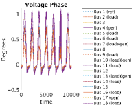
(f) Va buses 1-18

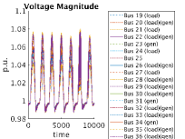
(g) Vm buses 19-36

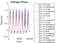
(h) Va buses 19-36

Figure 5: Smoothed and downsampled time series of the voltage time series and the power time series as solved by Matpower for the PFE of the IEEE-37 grid. Panels (a),(c) and (b),(d) depict the active and reactive power of buses 1-18 and 19-36, respectively. Panels (e),(g) and (f),(h) depict the voltage magnitudes and angles of buses 1-18 and 19-36, respectively. 1 p.u. equals to $4.8$ KV.

Based on the Matpower outputs, which include the full pre-processed time series of power and voltage phasors, we construct a data set for every pair of $\{T,N_{s}(t)\}$, which will be examined in the sequel. Specifically, we focus on the non observable situation of the SFSE scenario ($\mathcal{O}^{t}<\frac{1}{2}$ i.e., $\mathcal{O}^{t}<50\%$), where the number of the observable voltages at the time step $t$ is $N_{v}(t)=0$, and the number of the observable power phasors at the same time step is $0\leq N_{s}(t)<N$.

The data set construction began with randomly selecting a set of $9,000$ $T-$long sequences of time series from the available week-long data set. $8,100$ sequences (i.e., $90\%$) are drawn from the first six days, and are used for training the DNN, whereas the other $900$ sequences are drawn from the last day, to serve as a test set. Each sequence consists of (i) a fully observable $[T-1]$-long time series containing the power and voltage phasors for all nodes (i.e., $\underline{s}(\tau)$ and $\underline{v}(\tau)$ for $\tau{}\in{\{t-1-T,\cdots,t-1\}}$), (ii) a partially observable time step containing $N_{s}(t)$ power phasors, $\underline{s}(t)$, and (iii) a corresponding target voltage vector, $\underline{v}(t)$. Each power and voltage component (real and imaginary) in the data set was standardized using the mean and the standard deviation obtained from the training set. An illustration of the full data-preparation scheme is depicted in Fig. 6.

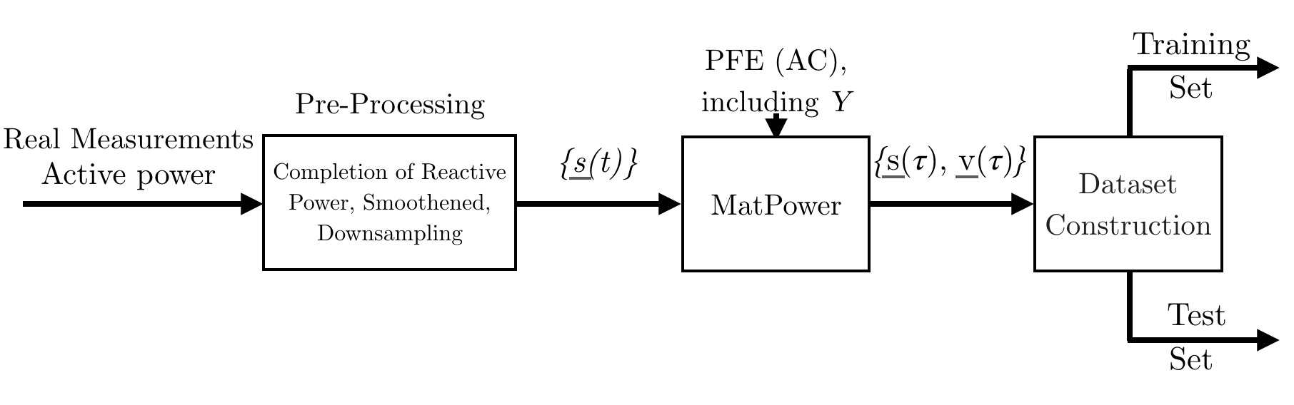
Figure 6: Illustration of the Data Preparation Scheme

III-B Training

We trained DNN using permutations of the following design parameters:

1. $T\in\{5,50\}$

2. $N_{s}(t)\in\{35,28,18,12,6\}$

3. $\lambda\in\{0,1,2,20\}$

giving a total of $40$ different permutations which cover $5$ different observability scenarios: $\mathcal{O}(35,0)=49\%$, $\mathcal{O}(28,0)=39\%$, $\mathcal{O}(18,0)=25\%$, $\mathcal{O}(12,0)=17\%$, $\mathcal{O}(6,0)=8\%$. In order to simulate a real-world scenario, increasing the number of buses that do not report the measurements (and thus, reducing the observability) was not selected randomly, but rather the observability was lost in a systematic method, based on the topological formation of the grid. That is, decreasing the observability was conducted by removing the information from buses located in the same area of the grid, starting from bus $\#36$ and advancing towards the reference bus, $\#1$. An example of $N_{s}(t)=28$ is illustrated in Fig. 7.

The training of the DNN for each of the different permutations was performed $30$ times, in order to obtain statistically significant results (each run with randomly selected (and thus, different) DNN weights initializations). The optimizer that was used during the training is the Adam optimizer [27], based on mini-batches of $50$ examples.

It is worth noting, that prior to the establishment of the full experimental setup, we conducted a trace-based simulation (based on parts of the available processed data sets) using Matpower case4 dist 4-buses distribution network scenario. Based on this simple trace-based simulation, we found the general values of the model design parameters (i.e., Number of layers in the fully connected modules, feature vector sizes, activation functions, $\lambda$, $T$), which was later used to design the full experiment. In other words, we preserved the same DNN architecture and design parameters of the 4-buses distribution network scenario when implementing the full experimental setup, up to minor feature vector resizing (due to the different input size).

III-C Evaluation

We evaluated the trained DNNs using the test-set data (which was taken from the last $1/7$ part ($900$ sequences) of the real-world data, and was not used for training). We then calculated the MSE of the resulting voltages estimates (for each of the permutations, the MSE was obtained by averaging across 30 runs). Although the data set is standardized and its values are in the rectangular complex format, we converted the MSE with respect to a de-standardized, polar representation (Magnitude, Angle) since this representation is more meaningful for practical uses. the estimated voltages are first de-standardized (by multiplying them by the standard deviation and adding a mean value) and then transformed to a polar format. Moreover, since we observed that the typical MSE of the magnitude values of the estimated voltages differs from the typical MSE of the angle of the estimated voltages by several orders of magnitudes, we analyzed the magnitude and the angle separately.

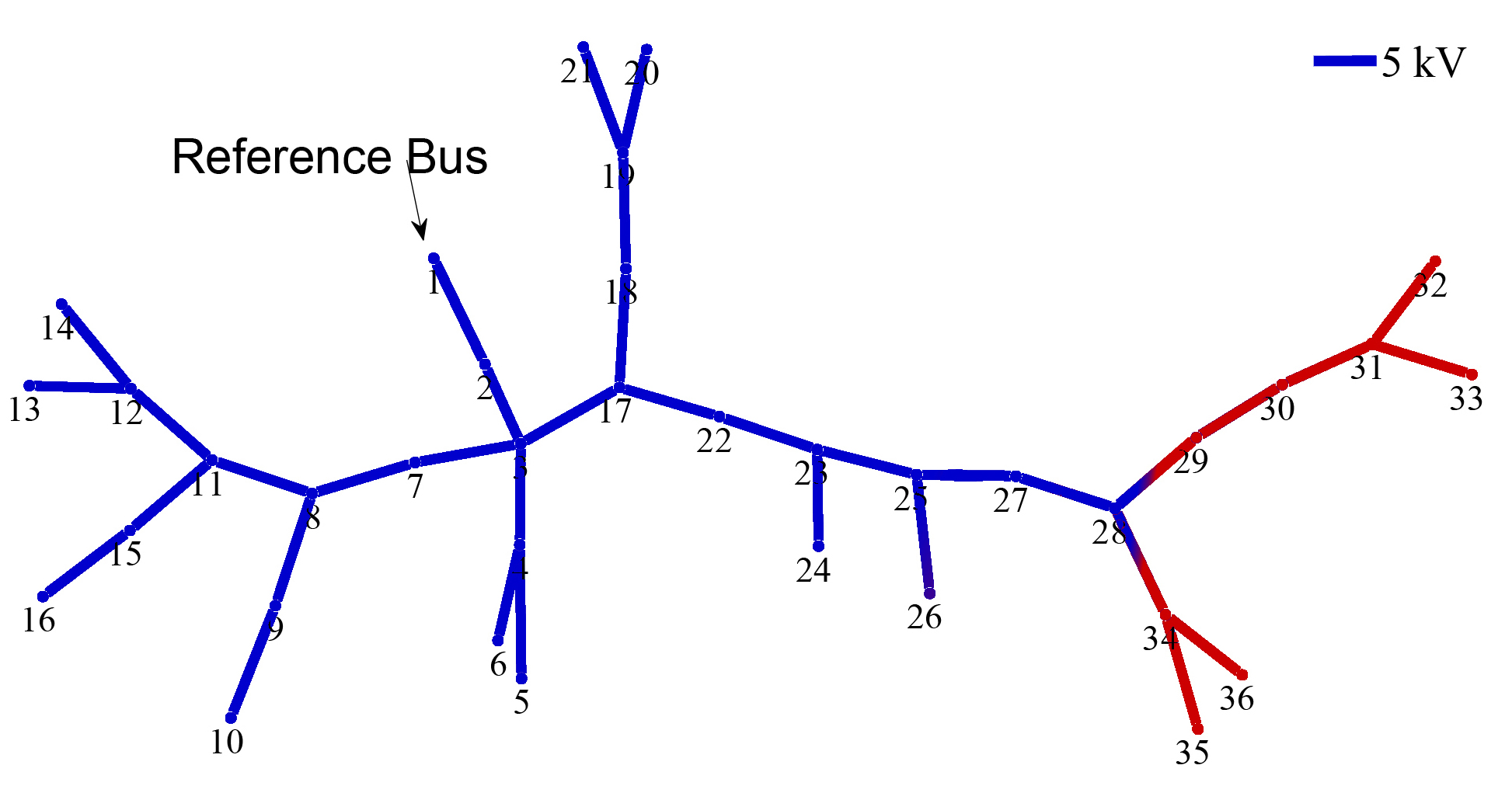
Figure 7: Illustration of the IEEE-37 Node test feeder, where none of the voltages phasors, $\underline{v}(t)$, are known, and part of the power information, $\underline{s}(t)$ is missing (the buses which do not report the power information are colored in red), giving an observability value of $\mathcal{O}^{t}=39\%$ (i.e., $N_{s}(t)=28;N_{v}(t)=0$). The buses that do not report the power information are selected based on their identification number (1-36).

III-D Results

The MSE values of the different estimates $\underline{\hat{v}}(t)$ for all permutations (for $T=5$) are plotted in Fig. 8. The MSE values as achieved by the standard WLS, including a persistence guess for all permutations (for $T=5$) are plotted in Fig. 9.

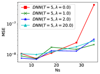
(a) Magnitude{$\underline{v}(t)$}

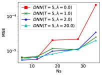
(b) Angle{$\underline{v}(t)$}

Figure 8: MSE for the IEEE-37 Node test feeder voltages magnitude and angle estimation under partial observability. This plot compares DNN models trained with different degree of PFE regularization.

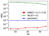
(a) Magnitude{$\underline{v}(t)$}

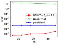
(b) Angle{$\underline{v}(t)$}

Figure 9: MSE for the IEEE-37 Node test feeder voltages magnitude and angle estimation under partial observability - WLS estimation and persistent guess. The DNN results (for $\lambda=2$) are plotted for comparison.

Looking at Fig. 8 and Fig. 9, we can clearly see that the DNN outperforms both the WLS-based estimation and the persistence guess by a big margin. Furthermore, the incorporation of the PFE information into the loss function as a regularizer (see (3)) further improves the accuracy of the estimates. This is especially evident in the estimation of the voltage-angles.

III-D1 Impact of the selected value of $\lambda$

A DNN trained with PFE regularization ($\lambda>0$) showed, in general, lower MSE when compared with a non-regularized DNN ($\lambda=0$). This phenomenon is especially evident in the angle estimation (see Fig. 9). Indeed, the improvement is less pronounced for the magnitude estimation. However, this can be explained by the fact that the MSE achieved by all DNN’s (including $\lambda=0$) is extremely small, and thus, the overall margin of improvement is narrower.

III-D2 Influence of the size of $T$

Fig. 10 presents a comparison between $T=5$ and $T=50$ for selected permutations. As can be seen, the differences are negligible. Thus, it can be concluded that the amount of information from historic data (with respect to future voltage-phasor estimation) is negligible beyond at least a 5-minute window ($T=5$).

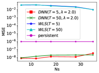
(a) Magnitude{$\underline{v}$}

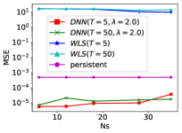
(b) Angle{$\underline{v}$}

Figure 10: Impact of $T$. The Y axis shows the MSE for the IEEE-37 Node test feeder voltages magnitude and angle estimation under partial observability. The plot compares the estimation MSE of DNN to WLS and persistent estimators. All the estimators were checked both with $T\in\{5,50\}$.

IV Conclusion and Discussion

In this paper, we presented a new approach of state-estimation in the distribution grids during sudden failures or attacks. The method capitalizes on a physics-informed DNN training algorithm that is able to take advantage of the grid physical information. We demonstrated the performance of the proposed method using an experimental setup which simulates a case of a sudden failure and loss of observability. We showed that our DNN-based estimation achieves a higher accuracy of the voltage-phasors estimation when compared with the widely used WLS-based estimation. Furthermore, the main contribution of incorporating the PFE regularization into the DNN model was shown to be in the voltage-angles estimation. The latter is typically overlooked in standard DSSE algorithms, but will become an important factor in modern and future low-inertia distribution grids.

Some ideas for further research follow: 1) Although our PFE-induced training of a DNN showed higher state estimation accuracies, we did not perform a full analysis study regarding the optimal value of $\lambda$ parameter for a given observability value ($\mathcal{O}^{t}$). The next step of our work is to establish a set of optimal $\lambda$ values. 2) Furthermore, in this paper we compared our physics-informed DNN output estimation accuracy to the standard WLS methodology which uses historic data in order to establish the different weighting of the missing samples. However, new approaches for the missing PMU data recovery [17] may be used in order to enhance both the WLS and our proposed DNN, which could improve the overall estimation accuracy, and should be investigated in future work. 3) In this research, we used the DNN model with real numbers. As the complex-number capable DNNs are currently being studied [28], it is worth investigating the DSSE problem based on a DNN over the $\mathbb{C}$ field. 4) Lastly, it is important to develop a unified DNN model that will be capable of dealing with multiple levels of observability without requiring dedicated training sessions.

References

- [1] A. Abur and A. G. Exposito, Power System State Estimation: Theory and Implementation. Abingdon: Dekker, 2004.
- [2] M. E. Baran, “Challenges in state estimation on distribution systems,” in 2001 Power Engineering Society Summer Meeting. Conference Proceedings (Cat. No.01CH37262), vol. 1, July 2001, pp. 429–433.
- [3] S. Soltan, M. Yannakakis, and G. Zussman, “REACT to cyber attacks on power grids,” IEEE Transactions on Network Science and Engineering, vol. 6, no. 3, pp. 459–473, 2018.
- [4] S. Soltan and G. Zussman, “EXPOSE the line failures following a cyber-physical attack on the power grid,” IEEE Transactions on Control of Network Systems, vol. 6, no. 1, pp. 451–461, 2019.
- [5] S. Soltan and G. Zussman, “Quantifying the effect of k-line failures in power grids,” in IEEE Power and Energy Society General Meeting (PESGM), July 2016.
- [6] J. Ostrometzky, A. Bernstein, and G. Zussman, “Irradiance field reconstruction from partial observability of solar radiation,” To appear in IEEE Geoscience and Remote Sensing Letters, 2019.
- [7] A. Primadianto and C. Lu, “A review on distribution system state estimation,” IEEE Transactions on Power Systems, vol. 32, no. 5, pp. 3875–3883, Sept. 2017.
- [8] G. Wang, G. B. Giannakis, J. Chen, and J. Sun, “Distribution system state estimation: an overview of recent developments,” Frontiers of Information Technology & Electronic Engineering, vol. 20, no. 1, pp. 4–17, Jan. 2019.
- [9] R. Singh, B. C. Pal, and R. B. Vinter, “Measurement placement in distribution system state estimation,” IEEE Transactions on Power Systems, vol. 24, no. 2, pp. 668–675, 2009.
- [10] S. Bhela, V. Kekatos, and S. Veeramachaneni, “Enhancing observability in distribution grids using smart meter data,” IEEE Transactions on Smart Grid, vol. 9, no. 6, pp. 5953–5961, 2018.
- [11] H. Jiang and Y. Zhang, “Short-term distribution system state forecast based on optimal synchrophasor sensor placement and extreme learning machine,” in IEEE Power and Energy Society General Meeting (PESGM), July 2016.
- [12] K. A. Clements, “The impact of pseudo-measurements on state estimator accuracy,” in IEEE Power and Energy Society General Meeting (PESGM), July 2011.
- [13] E. Manitsas, R. Singh, B. C. Pal, and G. Strbac, “Distribution system state estimation using an artificial neural network approach for pseudo measurement modeling,” IEEE Transactions on Power Systems, vol. 27, no. 4, pp. 1888–1896, Nov 2012.
- [14] J. Wu, Y. He, and N. Jenkins, “A robust state estimator for medium voltage distribution networks,” IEEE Transactions on Power Systems, vol. 28, no. 2, pp. 1008–1016, 2013.
- [15] P. Gao, M. Wang, S. G. Ghiocel, J. H. Chow, B. Fardanesh, and G. Stefopoulos, “Missing data recovery by exploiting low-dimensionality in power system synchrophasor measurements,” IEEE Transactions on Power Systems, vol. 31, no. 2, pp. 1006–1013, 2016.
- [16] C. Genes, I. Esnaola, S. M. Perlaza, L. F. Ochoa, and D. Coca, “Robust recovery of missing data in electricity distribution systems,” IEEE Transactions on Smart Grid, vol. 10, no. 4, pp. 4057–4067, 2019.
- [17] M. Liao, D. Shi, Z. Yu, Z. Yi, Z. Wang, and Y. Xiang, “An alternating direction method of multipliers based approach for pmu data recovery,” IEEE Transactions on Smart Grid, vol. 10, no. 4, pp. 4554–4565, 2019.
- [18] P. L. Donti, L. Yajing, A. J. Schmitt, A. Bernstein, Y. Rui, and Y. Zhang, “Matrix completion for low-observability voltage estimation,” arXiv preprint arXiv:1801.09799, 2018.
- [19] A. S. Zamzam and N. D. Sidiropoulos, “Physics-aware neural networks for distribution system state estimation,” arXiv preprint arXiv:1903.09669, 2019.
- [20] K. P. Schneider, B. A. Mather, B. C. Pal, C. . Ten, G. J. Shirek, H. Zhu, J. C. Fuller, J. L. R. Pereira, L. F. Ochoa, L. R. de Araujo, R. C. Dugan, S. Matthias, S. Paudyal, T. E. McDermott, and W. Kersting, “Analytic considerations and design basis for the ieee distribution test feeders,” IEEE Transactions on Power Systems, vol. 33, no. 3, pp. 3181–3188, 2018.
- [21] A. Bernstein, C. Wang, E. Dallanese, J.-Y. L. Boudec, and C. Zhao, “Load-flow in multiphase distribution networks: Existence, uniqueness, non-singularity, and linear models,” IEEE Transactions on Power Systems, pp. 1–1, 2017.
- [22] J. S. F.A. Gers and F. Cummins, “Learning to forget: continual prediction with lstm,” IET Conference Proceedings, pp. 850–855, 1999.
- [23] M. A. Nielsen, Neural networks and deep learning. Determination press San Francisco, CA, USA, 2015, vol. 2018.
- [24] J. Bank and J. Hambrick, “Development of a high resolution, real time, distribution-level metering system and associated visualization, modeling, and data analysis functions,” National Renewable Energy Lab.(NREL), Golden, CO (United States), NREL/TP-5500-56610,, Tech. Rep., 2013.
- [25] A. V. Oppenheim, Discrete-time signal processing. Pearson Education India, 1999.
- [26] R. D. Zimmerman, C. E. Murillo-Sánchez, and R. J. Thomas, “Matpower: Steady-state operations, planning, and analysis tools for power systems research and education,” IEEE Transactions on power systems, vol. 26, no. 1, pp. 12–19, 2010.
- [27] D. P. Kingma and J. Ba, “Adam: A method for stochastic optimization,” in 3rd International Conference on Learning Representations (ICLR), 2015.
- [28] C. Trabelsi, O. Bilaniuk, Y. Zhang, D. Serdyuk, S. Subramanian, J. F. Santos, S. Mehri, N. Rostamzadeh, Y. Bengio, and C. J. Pal, “Deep complex networks,” arXiv preprint arXiv:1705.09792, 2017.