Resolved observations at 31 GHz of spinning dust emissivity variations in $\rho$ Oph

Abstract

The $\rho$ Oph molecular cloud is one of the best examples of spinning dust emission, first detected by the Cosmic Background Imager (CBI). Here we present 4.5 arcmin observations with CBI 2 that confirm 31 GHz emission from $\rho$ Oph W, the PDR exposed to B-type star HD 147889, and highlight the absence of signal from S1, the brightest IR nebula in the complex. In order to quantify an association with dust-related emission mechanisms, we calculated correlations at different angular resolutions between the 31 GHz map and proxies for the column density of IR emitters, dust radiance and optical depth templates. We found that the 31 GHz emission correlates best with the PAH column density tracers, while the correlation with the dust radiance improves when considering emission that is more extended (from the shorter baselines), suggesting that the angular resolution of the observations affects the correlation results. A proxy for the spinning dust emissivity reveals large variations within the complex, with a dynamic range of 25 at 3$\sigma$ and a variation by a factor of at least 23, at 3$\sigma$, between the peak in $\rho$ Oph W and the location of S1, which means that environmental factors are responsible for boosting spinning dust emissivities locally.

1 Introduction

Since 1996, experiments designed to measure CMB anisotropies have found a diffuse foreground in certain regions of our Galaxy in the range of 10-60 GHz. For instance, the Cosmic Background Explorer (COBE) satellite measured a statistical correlation between the emission at 31.5 GHz and 140 $\upmu$m, at high Galactic latitudes and over large angular scales (Kogut et al., 1996). The spectral index of this radio-IR correlated signal was explained by a superposition of dust and free-free emission. Later, Leitch et al. (1997) detected diffuse emission at 14.5 GHz, which was spatially correlated with IRAS 100 $\upmu$m. This emission was 60 times stronger than the free-free emission and well in excess of the predicted levels from synchrotron and Rayleigh-Jeans dust emission, thus confirming the existence of an Anomalous Microwave Emission (AME).

The AME is a dust-correlated signal observed in the 10-100 GHz frequency range (see Dickinson et al. 2018 for a review). Numerous detections have been made in our Galaxy by separating the AME excess from the other radio components, namely synchrotron, free-free, CMB and thermal dust emission. It has been distinctly measured by CMB experiments and telescopes at angular resolutions of $\sim$ 1^∘; for instance, the WMAP (Bennett et al., 2013) and Planck (Planck Collaboration et al., 2013, 2014b) satellites have provided detailed information on diffuse emission mechanisms in the Galaxy through full-sky maps. Based on such surveys, AME accounts for $\approx$ 30$\%$ of the Galactic diffuse emission at 30 GHz (Planck Collaboration et al., 2014b). AME has also been observed in several clouds and Hii regions (e.g. Finkbeiner 2004; Watson et al. 2005; Casassus et al. 2006; Davies et al. 2006, Dickinson et al. (2007, 2009), Ami Consortium et al. 2009; Dickinson et al. 2009; Planck Collaboration et al. 2011; Vidal et al. 2011; Planck Collaboration et al. 2014c; Génova-Santos et al. 2015), some of them being arcminute resolution observations of well known regions (Casassus et al., 2008; Scaife et al., 2010a; Castellanos et al., 2011; Tibbs et al., 2011; Battistelli et al., 2015). There have been a few extra-galactic AME detections as well, such as in the galaxy NGC 6946 (Murphy et al., 2010a; Scaife et al., 2010b; Hensley, Murphy & Staguhn, 2015; Murphy et al., 2018) and M 31 (Planck Collaboration et al., 2015; Battistelli et al., 2019). Although, extra-galactic studies are still a challenge due to the diffuse nature of the emission.

AME is thought to originate from dust grains rotating at GHz frequencies and emitting as electric dipoles. Long before its detection, Erickson (1957) proposed that electric dipole emission from spinning dust grains could produce non-thermal radio emission. Draine & Lazarian (1998a) calculated that interstellar spinning grains can produce emission in the range from 10 to 100 GHz, at levels that could account for the AME. Since then, additional detailed theoretical models have been constructed to calculate the spinning dust emission, taking into account all the known physical mechanisms that affect the rotation of the grains. The observed spectral energy distributions (SEDs) of a number of detections are a qualitative match to spinning dust models (e.g. Planck Collaboration et al., 2014c). Thus, the spinning dust (SD) hypothesis has been the most accepted to describe the nature of the AME.

As SD emission depends on the environmental conditions, a quantitative comparison between AME observations and synthetic spectra can give us information on the local physical parameters. However, even when there is a dependence on the environmental parameters, variations over a wide range of environmental conditions (e.g. typical conditions for a dark cloud versus a photo-dissociation region) only produce emissivity changes smaller than an order of magnitude (e.g. Draine & Lazarian, 1998b; Ali-Haïmoud, Hirata & Dickinson, 2009). Although, greater changes in SD emissivity models are observed by varying parameters intrinsic to the grain population, as shown by Hensley & Draine (2017a), where they highlighted the importance of grain size, electric dipole and grain charge distributions. Observationally, Tibbs et al. (2016) and Vidal et al. (2020) reported that they can only explain SD emissivity variations in different clouds by modifying the grain size distribution for the smallest grains.

Within the SD model, the smallest grains are the largest contributors to the emission. These have sub-nanometer sizes and spin at GHz frequencies. Polycyclic Aromatic Hydrocarbons (PAHs) are natural candidates for the AME carriers, as they are a well established nanometric-sized dust population (Tielens, 2008), and correlations between AME and PAHs tracers have been observed (Scaife et al., 2010a; Ysard, Miville-Deschênes & Verstraete, 2010; Tibbs et al., 2011; Battistelli et al., 2015). However, a full-sky study by Hensley, Draine & Meisner (2016) found a lack of correlation between the Planck AME map and a template of PAH emission constructed with 12 $\upmu$m data. Tibbs et al. (2013) found that in Perseus Very Small Grains (VSGs) emission at 24 $\upmu$m is more correlated with AME than 5.8 $\upmu$m and 8 $\upmu$m PAH templates. Recently, Vidal et al. (2020) confirmed that 30 GHz AME from the translucent cloud LDN 1780 correlates better with a 70 $\upmu$m map. Rotational nanosilicates have also been considered as the carriers of the AME and they can account for all the emission without the need of PAHs (Hoang, Vinh & Quynh Lan, 2016; Hensley & Draine, 2017b). These results have raised questions about the PAHs hypothesis as the unique carriers of AME.

One of the key characteristics of AME, based on observations, is that it seems to be always connected with photo-dissociation regions (PDRs). PDRs are optimal environments for SD production (Dickinson et al., 2018): there is high density gas, presence of charged PAHs and a moderate interstellar radiation field (ISRF) that favours an abundance of small particles due to the destruction of large grains. For instance, Pilleri et al. (2012) fitted ISO mid-IR spectra and showed that an increasing UV-radiation field in PDRs favours grains destruction. Also, Habart et al. (2003) used ISO observations and concluded that the emission in the $\rho$ Oph W PDR is dominated by the photoelectric heating from PAHs and very small grains. The most significant AME detections have been traced back to PDRs (Casassus et al., 2008; Planck Collaboration et al., 2011; Vidal et al., 2020).

Among the most convincing observations on the SD hypothesis is the $\rho$ Ophiuchi ($\rho$ Oph) molecular cloud, an intermediate-mass star forming region and one of the brightest AME sources in the sky (Casassus et al., 2008; Planck Collaboration et al., 2011). The region of $\rho$ Oph exposed to UV radiation from HD 147889, the earliest-type star in the complex, forms a filamentary PDR whose brightest regions in the IR include the $\rho$ Oph W PDR (Liseau et al., 1999; Habart et al., 2003). $\rho$ Oph W is the nearest example of a PDR, at a distance of 134.3 $\pm$ 1.2 pc in the Gould Belt (Gaia Collaboration et al., 2018). In radio-frequencies, observations with the Cosmic Background Imager (CBI) by Casassus et al. (2008) showed that the bright cm-wave continuum from $\rho$ Oph, for a total WMAP 33 GHz flux density of $\sim$20 Jy, stems from $\rho$ Oph W and is fitted by SD models. They found that the bulk of the emission does not originate from the most conspicuous IR source, S1. This motivated the study of variations of the SD emissivity per H-nucleus, $j_{\nu}$ = $I_{\nu}/N_{\mathrm{H}}$, which at the angular resolutions of their observations led to the tentative detection of $j_{\nu}$.

In this work, we report Cosmic Background Imager 2 (CBI 2) observations of $\rho$ Oph W, at a frequency of 31 GHz and an angular resolution of 4.5 arcmin. In relation to the CBI, this new data-set provides a finer angular resolution by a factor of 1.5 and better surface brightness sensitivity. Section 2 of this paper describes the CBI 2 characteristics and observations, as well as the ancillary data. Sec. 3 presents a qualitative analysis of the IR/radio features of the PDR. In Sec. 4 we describe the results of the correlation analysis between the 31 GHz data and the different IR and column density templates, and in Sec. 5 we analyse the size variations of the PAHs in the PDR. In Sec. 6 we quantify the SD emissivity variations throughout $\rho$ Oph and discuss the implications of our results, and Sec. 7 concludes.

2 The data

2.1 Cosmic Background Imager 2 Observations

The observations at 31 GHz were carried out with the Cosmic Background Imager 2 (CBI 2), an interferometer composed of 13 Cassegrain antennae (Taylor et al., 2011). The CBI 2 is an upgraded version of the Cosmic Background Imager (CBI, Padin et al., 2002). In 2006, the antennae were upgraded from 0.9 m (CBI) to 1.4 m dishes (CBI 2). As opposed to the CBI, CBI 2 has an increased surface brightness sensitivity at small angular scales due to the incorporation of larger dishes that provide a better filling factor for the array. Technical specifications of the CBI and CBI 2 are presented in Table 1.

Table 1: Technical specifications for the CBI and CBI 2.

	CBI	CBI 2
Years of operation	1999-2006	2006-2008
Observing frequencies (GHz)	26-36	26-36
Number of antennae	13	13
Number of channels (1 GHz)	10	10
Number of baselines	78	78
Antenna size (m)	0.9	1.4
Primary beam FWHM (arcmin)	45	28.2

The observations were spread over 27 days in March of 2008. We acquired data distributed in 6 pointings: 1 pointing centered at the $\rho$ Oph W PDR, 3 pointings defined around the PDR, and 2 more pointings centered at stars S1 and SR3. Table 2 shows the coordinates for each pointing, as well as their respective RMS noise. The data-set was reduced using the standard CBI pipeline (CBICAL) and software (Pearson et al., 2003; Readhead et al., 2004a, b), with Jupiter as the main flux calibrator. As the CBI 2 is a co-mounted interferometer, the pointing error associated with each antenna has to be accounted by the combined pointing error of the baseline pairs of antennae. This yields a residual pointing error of $\sim$ 0.5 arcmin (Taylor et al., 2011).

Table 2: Coordinates for the observation of the $\rho$ Oph W PDR and the pointings defined around it. S1 and SR3 are the early-type stars of interest. The angular resolution of the observation is 4.5 arcmin.

	RAa	DECb	RMS [mJy beam-1]
$\rho$ Oph W PDR	16:25:57.0	$-$24:20:48.0	6.7
$\rho$ Oph 1	16:26:06.0	$-$24:37:51.0	9.3
$\rho$ Oph 2	16:26:00.0	$-$24:22:32.0	30.2
$\rho$ Oph 3	16:25:14.0	$-$24:11:39.0	15.0
$\rho$ Oph S1	16:26:34.18	$-$24:23:28.33	12.7
$\rho$ Oph SR3	16:26:09.32	$-$24:34:12.18	9.6

• J2000. Right ascension are in HMS and Declinations are in DMS.

2.2 Image reconstruction

We considered two approaches to reconstruct an image from the CBI 2 data. One of them is the traditional clean algorithm, in which we used a Briggs robust 0 weighting scheme to construct a continuum mosaic. Figure 1 shows the reconstructed mosaic using the CASA 5.1 clean task (McMullin et al., 2007). This mosaic shows the location of the 3 early-type stars in the field - HD 147889, S1 and SR3. It also presents the 31 GHz intensity contours at 3$\sigma$, 5$\sigma$, 10$\sigma$, 15$\sigma$ and 20$\sigma$, for an RMS noise of $\sigma\approx$0.01 Jy beam^-1. The dashed circle represents the 28.2 arcmin primary beam of the central pointing ($\rho$ Oph W PDR in Table 2), and the bottom left green ellipse shows the synthesized primary beam, with a size of 4.6 $\times$ 4.0 arcmin.

Figure 1: Mosaic of the 31 GHz continuum measured by CBI 2 in units of Jy beam^-1. This image was reconstructed using the CASA clean task. The RMS noise is $\sigma\approx$0.01 Jy beam^-1 and we show intensity contours for 3$\sigma$, 5$\sigma$, 10$\sigma$, 15$\sigma$ and 20$\sigma$. The star markers indicate the three early-type stars in the field: S1, SR3 and HD 147889. We also detected radio galaxy PMN J1626-2426 (labeled in the figure). The CBI 2 synthesized beam (4.6 $\times$ 4.0 arcmin) is shown as a green ellipse on the bottom left and the primary beam for the main pointing (28.2 arcmin FWHM) is shown as a dashed circle.

Table 3: Flux densities and spectral indexes for source PMN J1626-2426, detected at RA 16:27:01.8, DEC -24:26:33.7 (J2000). The spectral index follows the convention S_ν $\propto$ $\nu^{\alpha}$ and it was calculated between the 31 GHz flux from the clean map and the catalogued fluxes. The reported fluxes correspond to different epochs, indicating variability in the spectrum.

Observing Frequency [GHz]	Flux Density [mJy]	$\alpha_{(\nu/31\,\mathrm{GHz})}$
1.4	57.2 $\pm$ 1.8 a	0.01 $\pm$ 0.03
4.8	132 $\pm$ 13 b	-0.43 $\pm$ 0.07
8.4	77.9 c	-0.21
20	78 $\pm$ 5 d	-0.61 $\pm$ 0.25
31	59.6 $\pm$ 5.3 e	-

• Reported in Condon et al. (1998).

• Reported in Griffith et al. (1994).

• Reported in Sowards-Emmerd et al. (2004). Error not reported.

• Reported in Murphy et al. (2010b).

• Reported in this work.

In a second approach we used an alternative image reconstruction strategy, based on non-parametric image deconvolution, as in the maximum-entropy method (following the algorithms described in Casassus et al., 2006, 2008). Here we used the gpu-uvmem package (Cárcamo et al., 2018), implemented in GPU architectures. Thanks to entropy regularization and image positivity, the model image can super-resolve the clean beam, in the sense that its effective angular resolution is $\sim$1/3 that of the natural-weighted beam (so even finer than uniform weights). To obtain a model sky image that fits the data we need to solve the usual deconvolution problem, i.e. obtain the model image $I^{m}$ that minimize a merit function $L$:

$$L=\chi^{2}-\lambda\sum_{i}p_{i}\ln(p_{i}/M),$$ (1)

where

$$\chi^{2}=\frac{1}{2}\sum_{k=0}^{N}\omega_{k}||V_{k}^{\circ}-V_{k}^{m}||^{2}.$$ (2)

Here, $V_{k}^{\circ}$ are the observed visibilities, each with weight $\omega_{k}$, and $V_{k}^{m}$ are the model visibilities calculated on the model images. The optimization is carried out by introducing the dimensionless free parameters $p_{i}=I_{i}/\sigma_{D}$, and $M$ is the minimum value for the free parameters. In this case, we set $M$ = $10^{-3}$ and $\lambda$ = 2 $\times$ 10^-2. The gpu-uvmem algorithm also estimates a theoretical noise map as

$$\sigma=\sqrt{\frac{1}{\sum_{p=1}^{P}\overline{A}^{2}_{p}/\hat{\sigma}^{2}}}\,,$$ (3)

where $P$ is the number of pointings, $\overline{A}_{p}=\sum_{f=1}^{F}{A_{\nu_{f}}}/F$ is the mean of the primary beams over all frequencies $\{\nu_{f}\}_{f=1}^{F}$ available in pointing $p$, and $\hat{\sigma}$ is the noise on the dirty map using natural weights. Error propagation in the dirty map yields:

$$\hat{\sigma}=\sqrt{\frac{1}{\sum_{k}\omega_{k}}}\,.$$ (4)

In order to avoid an under-estimation of errors, we scaled the noise map so that its minimum value would match the RMS noise of the natural-weighted clean map. In increasing the noise level we also included a correction for the number of correlated pixels in both maps, i.e. the noise in the gpu-uvem model image is increased by $\sqrt{N_{\mathrm{clean}}/N_{\mathrm{uvmem}}}\sim 3$, where $N_{\mathrm{clean}}$ and $N_{\mathrm{uvmem}}$ are the number of pixels in each clean beam, and that of gpu-uvmem being $\sim$3 times smaller than the natural-weight beam.

In our analysis, we used both the clean and gpu-uvmem maps. The clean map was used to measure the correlation of the 31 GHz emission with the IR templates and the proxies for PAHs. We did not use the gpu-uvmem map to perform the correlations as it has a variable angular resolution. Instead, as the gpu-uvmem map recovers the morphology of the 31 GHz emission in detail, we used it to construct an emissivity proxy to analyse the emissivity variations throughout the PDR.

In our reconstructed clean mosaic we detected a point source located at RA 16:27:01.8, DEC -24:26:33.7 (J2000) that corresponds to the radio galaxy PMN J1626-2426 (labeled in Figure 1). This source is described in the PMN catalogue as a Flat Spectrum Radio Source, located at RA 16:27:00.01, DEC -24:26:40.50 (J2000) (Healey et al., 2007). In Table 3 we report the flux and spectral index (S_ν $\propto$ $\nu^{\alpha}$) of this point source at 31 GHz, along with catalog measurements at other frequencies. We measured the flux at 31 GHz using aperture photometry with a circular aperture of radius 2.5 arcmin. It is interesting to point out that this source has a Fermi detection of 0.35 $\pm$ 0.04 pJy at 50 GeV (Nolan et al., 2012), observed during 2008 and 2010. Its radio spectrum shows variability, especially considering the flux difference between the 1.4 GHz data, observed during 1993, and the 4.8 GHz data, observed during 1990 (see Table 3). The 8.4 GHz and 20 GHz data were taken during 2003 and 2006, respectively.

2.3 Ancillary Data

Table 4: Summary of the ancillary data.

Instrument	Wavelength [$\upmu$m]	Description
Spitzer-IRAC	8	Tracer for PAHsa.
WISE	3.4, 12	Tracer for PAHsa.
WISE	22	Tracer for VSGs.
Spitzer-MIPS	24	Tracer for VSGs.
Herschel-SPIRE	250	Tracer for big classical grains b

• In $\rho$ Oph W, this bands are dominated by PAHs. The 3.4$\upmu$m map is a better tracer for the smallest PAHs.

• Grains with sizes of $\sim$ hundreds of nm in thermal equilibrium.

The Wide-Field Infrared Survey Explorer (WISE) has surveyed the entire sky in four near-IR and mid-IR band-passes (Wright et al., 2010). Its near-IR survey at 3.4, 4.6 and 12 $\upmu$m gives information on the emission from VSGs and PAHs in the interstellar medium. We worked with the 3.4 $\upmu$m map, and the 12 $\upmu$m processed map by Meisner & Finkbeiner (2014), who smoothed the data-set to an angular resolution of 15 arcsec and removed the compact sources and optical artifacts from the image. We also used their map at 22 $\upmu$m for comparison purposes.

Dust grain tracers were also obtained from the InfraRed Array Camera ($\mathrm{IRAC}$) maps from the Spitzer Space Telescope survey. $\mathrm{IRAC}$ is a mid-IR camera with four channels at 3.6, 4.5, 5.8, and 8 $\upmu$m (Fazio et al., 2004). In this case, we used the 8 $\upmu$m template. The original data-set is presented in units of MJy sr^-1 and at an angular resolution of $\sim$ 2 arcsec. We also used the 24 $\upmu$m data-set from the Spitzer Multiband Imaging Photometer ($\mathrm{MIPS}$) (Rieke et al., 2004). This photometer works at 24, 70 and 160 $\upmu$m, producing maps with a native angular resolution between 6 and 40 arcsec.

In the particular case of $\rho$ Oph W, both 8 $\upmu$m and 12 $\upmu$m bands are dominated by PAHs. Given the radiation field in HD 147889 ($\chi$ $\sim$ 400, Habart et al., 2003) and for typical dust models (Draine & Li, 2007; Compiègne et al., 2011), we expect both bands to be tracing primarily PAHs.

To study the thermal dust emission we used data from the Herschel Gould Belt survey, which provides an extensive mapping of nearby molecular clouds, including detailed templates of $\rho$ Oph (André et al., 2010; Pilbratt et al., 2010). Specifically, we used data from the Spectral Photometric Imaging Receiver ($\mathrm{SPIRE}$), a three-band camera and spectrometer that works at 250, 350 and 500 $\upmu$m (Griffin et al., 2010). We also worked with the dust temperature data-set from the Photodetector Array Camera and Spectrometer ($\mathrm{SPIRE-PACS}$), that has a native angular resolution of 36.3 arcsec (Ladjelate et al., 2020). A summary of our ancillary data is presented in Table 4.

3 Qualitative radio/IR comparisons

Figure 2: Overview of $\rho$ Oph. Red: SPIRE 250 $\upmu$m, green: MIPS 24 $\upmu$m, blue: IRAC 8 $\upmu$m (PDR). The center of the image is at RA 16:25:55.20, DEC -24:25:48.0 (J2000). The markers indicate the locations of the 3 early-type stars in the field. Contours follow a gpu-uvmem model of the 31 GHz continuum measured by the CBI 2, at 30$\%$, 50$\%$, 70$\%$ and 90$\%$ of the emission peak at 0.51 Jy beam^-1. The white dashed arrow indicates the direction of the cut used to construct the emission profiles of the templates.

In Figure 2 we compare the CBI 2 31 GHz emission reconstructed with the gpu-uvmem algorithm (Sect. 2.2) shown in contours, with the $\mathrm{IRAC}$ 8 $\upmu$m in blue colour stretch, $\mathrm{MIPS}$ 24 $\upmu$m in green, and $\mathrm{SPIRE}$ 250 $\upmu$m in red. The 8 and 24 $\upmu$m templates trace the emission of small hot grains (sub-nm and nm-sizes), while the 250 $\upmu$m template traces thermal dust emission, mainly from big classical grains (size of hundreds of nm). In particular, the $\mathrm{IRAC}$ 8 $\upmu$m template is a main tracer of PAHs in this region.

The black markers in Fig. 2 show the position of the three early-type stars in $\rho$ Oph. S1 is a binary system composed of a B4V star and a K-type companion, with an effective temperature of $T_{\mathrm{eff}}\approx$ 15800 K. SR3, also known as Elia 2-16, is a B6V star with an effective temperature of $T_{\mathrm{eff}}\approx$ 14000 K. HD 147889, the main ionizing star of $\rho$ Oph, is catalogued as a single B2III/B2IV star (C-ionizing, Houk & Smith-Moore, 1988), with $T_{\mathrm{eff}}\approx$ 23000 K (Bondar, 2012). This star is heating and dissociating gas layers creating an Hii region of $\sim$ 6 arcmin towards the PDR traced by the free-free continuum in the PMN (Parkes-MIT-NRAO) 4.85 GHz map, and by the H$\alpha$ emission in SHASSA (Casassus et al., 2008). In Figure 3(a) we show normalized emission profiles for the IR templates and the 31 GHz data, for a cut starting from HD 147889 and passing through the 31 GHz emission peak, as shown by the dashed arrow in Fig. 2. We also plot the emission profile from the PMN 4.85 GHz map as a tracer of the free-free emission throughout the region. We find that, indeed, most of the 4.85 GHz emission comes from the vicinity of HD 147889. The 24 $\upmu$m map in Fig. 2 also shows thermal emission from hot grains near HD 147889. Towards the PDR (at $\sim$ 6 arcmin in Figure 3) and through the peak of the 31 GHz emission, the 4.85 GHz emission decreases, reaching the noise level of the original map. This lack of free-free emission at the location of the PDR can also be seen in the 1.4 GHz and H$\alpha$ maps of $\rho$ Oph presented in Planck Collaboration et al. (2011).

An interesting aspect of Fig. 2 is that the 31 GHz contours fall in the transition between small hot grains and bigger colder grains (reflected in the layered structure of the IR tracers, as also seen in Fig. 3(a)). This transition occurs at the PDR, where neutral Hydrogen becomes molecular. Deeper into the molecular core, away from HD 147889 in Fig. 2, the UV radiation field is attenuated, and the emergent emission progressively shifts towards 250 $\upmu$m.

Figure 3(a) shows that $\mathrm{IRAC}$ 8 $\upmu$m and $\mathrm{WISE}$ 12 $\upmu$m have a wider radial profile than that at 31 GHz, ranging from their peak at $\sim$5 arcmin distance from HD 147789 up to $\sim$15 arcmin. Note that around 5 arcmin there is a slight hump on the 31 GHz profile that matches the peak of $\mathrm{IRAC}$ 8 $\upmu$m. Also, at $\sim$10 arcmin, the $\mathrm{WISE}$ 12 $\upmu$m profile shows a hump at the position of the 31 GHz peak. This correlations might imply a relation between the rotational excitement of dust grains that originate the SD emission and the vibrational states of the small grains seen in the 8 $\upmu$m and 12 $\upmu$m profiles.

We note that the most conspicuous feature in the IR-map in Fig. 2, the circumstellar nebula around S1, shows a very faint 31 GHz counterpart. This is particularly interesting as Spitzer IRS spectroscopy shows very bright PAHs bands in the nebulae around S1 and SR3, as well as in the $\rho$ Oph W PDR (Habart et al., 2003; Casassus et al., 2008). This means that PAHs are not depleted around S1 and SR3, thus making the faint 31 GHz emission intriguing. Motivated by this, we performed a correlation analysis in order to quantify the best tracer of the 31 GHz emission throughout the region.

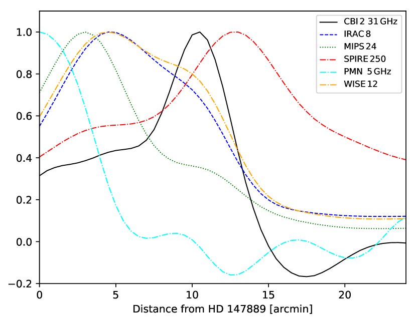
(a)

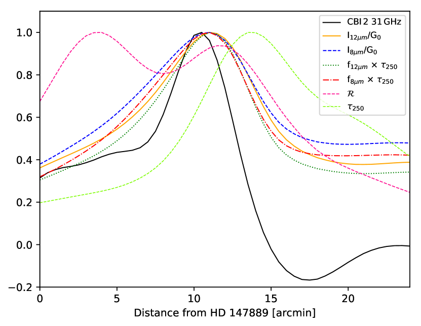
(b)

Figure 3: Normalized emission profiles vs. distance to ionizing star HD 147889. The profile cut, as shown by the dashed arrow in Fig. 2, was extracted starting from star HD 147889 and crossing the 31 GHz emission peak.

4 Correlation Analysis

We study the morphological correlation between the 31 GHz data and different IR maps that trace PAHs and VSGs. In order to avoid biases due to image reconstruction, we performed the correlations in the visibility ($uv$) plane. To transform our data-set to the $uv$-plane we used the $\mathrm{MOCKCBI}$ software from the CBI software tools. This program calculates the visibilities by Fourier-transforming a supplied map of the sky emission, in this case, various IR templates. To do this, all templates were reprojected to a 1024 $\times$ 1024 grid. In case that any of the original templates were of a smaller size, a noise gradient, calculated with the RMS noise limits of each map, was added to the borders. This is an important step to consider, otherwise, the resulting visibility maps would show an abrupt step towards its borders, producing artefacts in the mock visibilities. To visualize and compare the trend of our results we also calculated the correlations in the plane of the sky. We smoothed all the templates to 4.5 arcmin in order to fit CBI 2’s angular resolution. All templates were re-gridded to $\sim$ 3 pixels per beam to avoid correlated pixels.

4.1 PAH column density proxies

For the correlation analysis, we constructed proxies for the column density of PAHs. The mid-IR dust emission, due to PAHs, depends on the column density of the emitters and on the intensity of the local UV radiation, which can be quantified in units of the ISRF in the solar neighbourhood as the dimensionless parameter G₀ (Sellgren et al., 1985; Draine & Li, 2007). If the observed 31 GHz emission corresponds to SD emission, a stronger correlation is expected with the mid-IR emission when divided by G₀, as this will trace the column density of PAHs.

The radiation field intensity was estimated using the equation given by Ysard, Miville-Deschênes & Verstraete (2010):

$$G_{0}\,=\,\left(T_{\mathrm{dust}}/17.5K\right)\,^{\beta_{\mathrm{dust}}+\ 4}.$$ (5)

This method derives from radiative equilibrium with a single grain size of 0.1 $\upmu$m and an emissivity index $\beta_{\rm dust}$ = 2, which is constant across the field. As $\beta_{\rm dust}$ may vary throughout the PDR, a constant $\beta$ might not be a good approximation for G₀. We estimated the impact of variable $\beta_{\rm dust}$ in Eq. 5. We created a map of $\beta_{\rm dust}$ and T_dust by fitting a Modified Black Body to the far-IR data. For this, we used Herschel data at 100, 160, 250, 350 and 500 $\upmu$m. This fit results in $\beta_{\rm dust}$, $\tau$ and T_dust maps that would let us identify variations in the PDR at 4.5 arcmin. The resulting G₀ map, calculated with the variable $\beta_{\rm dust}$ and T_dust maps from the fit, is morphologically equivalent to the G₀ estimation using a constant $\beta_{\rm dust}$ and Herschel’s T_dust map. The Pearson correlation coefficient is $r$ = 0.95 $\pm$ 0.02 between both G₀ estimations. In this work, we are interested in comparing the morphology of the cm-wavelength (31 GHz) signal with that of the average radiation field along the line of sight. A 3D radiative transfer model that accounts for the IR spectral variations would provide an accurate estimation of the 3D UV radiation field (G₀(${\vec{x}}$)) and of the dust abundances (e.g., as in Galliano, 2018). Such modeling is beyond the scope of this work.

In stochastic heating, we expect the intensity of the IR bands due to PAHs to be approximately proportional to both the UV field intensity and the PAH column, so that (as in Casassus et al., 2008):

$$\frac{I_{\nu\,\mathrm{PAH}}}{G_{0}}\propto N_{\mathrm{PAH}}.$$ (6)

As templates for the PAHs emission, $I_{\nu\,\mathrm{PAH}}$, we used the $\mathrm{WISE}$ 12 $\upmu$m and $\mathrm{IRAC}$ 8 $\upmu$m intensity maps.

Another way to obtain a proxy for the column of PAHs, proposed by Hensley, Draine & Meisner (2016), is to correct I${}_{\nu\,\mathrm{PAH}}$ by the dust radiance ($\mathcal{R}$) as a method to quantify the fraction of dust in PAHs ($f_{\mathrm{PAH}}$). The dust radiance corresponds to the integrated intensity, $\mathcal{R}$ = $\int_{\nu}I_{\nu}$. We calculated this expression by considering a modified blackbody as in Planck Collaboration et al. (2014a, equation 10):

$$\mathcal{R}=\tau_{250}\frac{\sigma_{S}}{\pi}\,T^{4}_{\mathrm{dust}}\left(\frac{kT_{\mathrm{dust}}}{h\nu_{0}}\right)^{\beta_{\mathrm{dust}}}\,\frac{C(4+\beta_{\mathrm{dust}})\,\zeta(4+\beta_{\mathrm{dust}})}{\Gamma(4)\,\zeta(4)},$$ (7)

where $\tau_{\mathrm{250}}$ is the optical depth at 250 $\upmu$m, calculated using $\tau_{\mathrm{250}}$ = $I_{\mathrm{250\,\upmu m}}/B_{\mathrm{250\,\upmu m}}(T)$ by assuming an optically-thin environment. Also, $\nu_{0}$ is the frequency for 250 $\upmu$m, $\sigma_{S}$ is the Stefan-Boltzmann constant, $k$ is the Boltzmann constant, $h$ is the Planck constant and $\Gamma$ and $\zeta$ are the Gamma and Riemann-zeta functions, respectively. To recover the intensity units of the radiance map, we divide it by $\nu_{0}$, getting as a result $\mathcal{R}$/$\nu$. Hence, the PAH fraction can be calculated as:

$$\frac{\nu\,I_{\nu\,\mathrm{PAH}}}{\mathcal{R}}\propto f_{\mathrm{PAH}}.$$ (8)

Thus, the product of the PAH fraction times the optical depth will be proportional to the PAH column density:

$$f_{\mathrm{PAH}}\,\times\,\tau_{250}\propto N_{\mathrm{PAH}}.$$ (9)

We note that Hensley, Draine & Meisner (2016) stress the need of a good correlation between the mid-IR map and $\mathcal{R}$, which is the case of our 4.5 arcmin I${}_{\nu\,\mathrm{PAH}}$ and $\mathcal{R}$ maps, with correlation coefficients $r$ > 0.6. In Figure 4 we show a close-up of the 31 GHz clean mosaic, along with the column density proxies constructed with $\mathrm{WISE}$ 12 $\upmu$m and $\mathrm{IRAC}$ 8 $\upmu$m, and the radiance map.

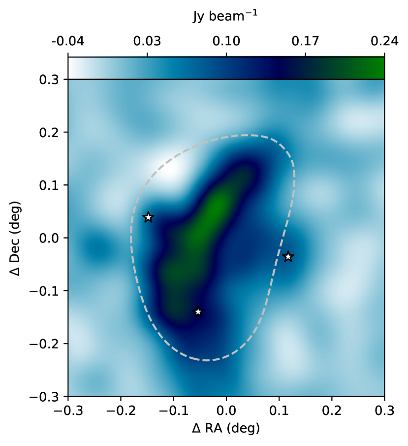
(a) CBI 2 31 GHz

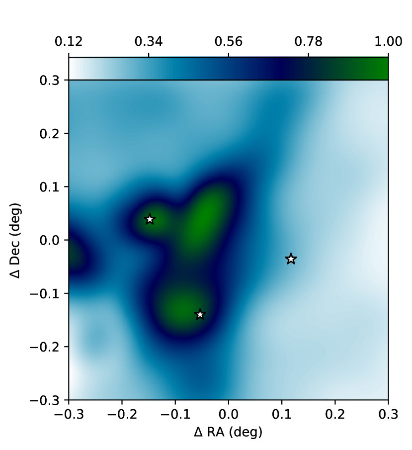
(b) $f_{\mathrm{\,12\,\upmu m}}\,\cdot\,\tau_{250}$

(c) $f_{\mathrm{8\,\upmu m}}\,\cdot\,\tau_{250}$

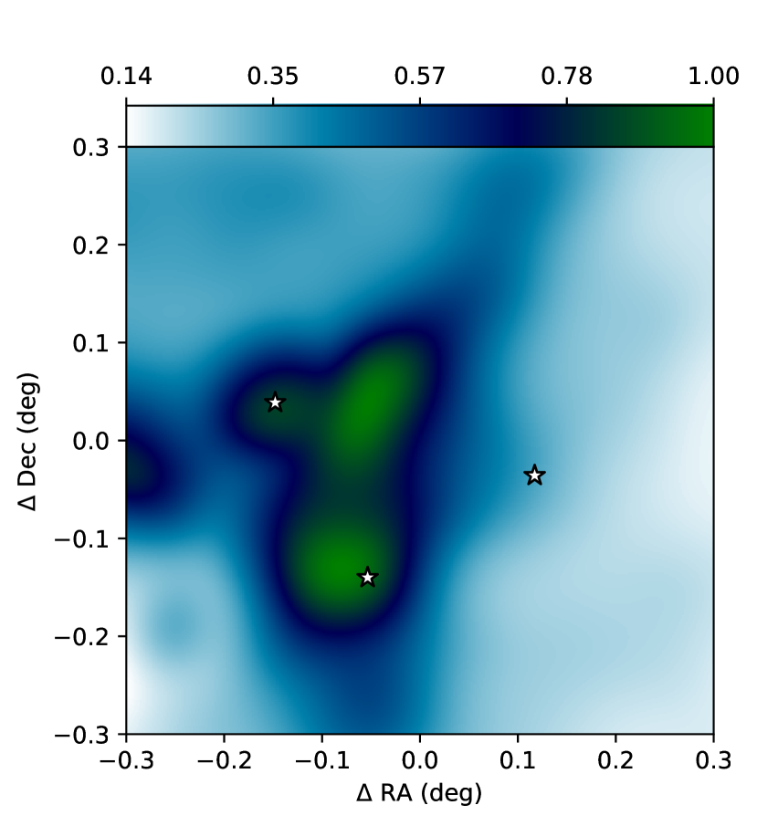
(d) I${}_{\mathrm{12\,\upmu m}}/G_{0}$

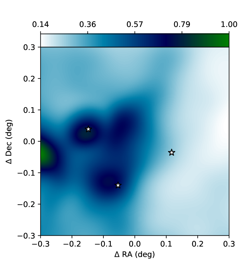
(e) I${}_{\mathrm{8\,\upmu m}}/G_{0}$

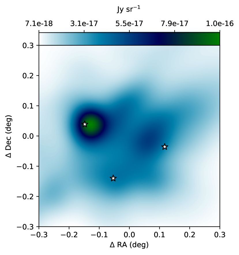
(f) $\mathcal{R}$/$\nu$

Figure 4: clean 31 GHz map (4(a), close-up from Fig. 1), normalized proxies for PAHs column densities (4(b)-4(e)) and radiance map (4(f)). The proxies for column densities correlate better with the 31 GHz data, and the morphology between them is very similar. In 4(a), the dashed region shows the area within which we calculated the plane of the sky correlations; it corresponds to 50$\%$ of the mosaic’s primary beam. The position for the three early-type stars are also marked in each map.

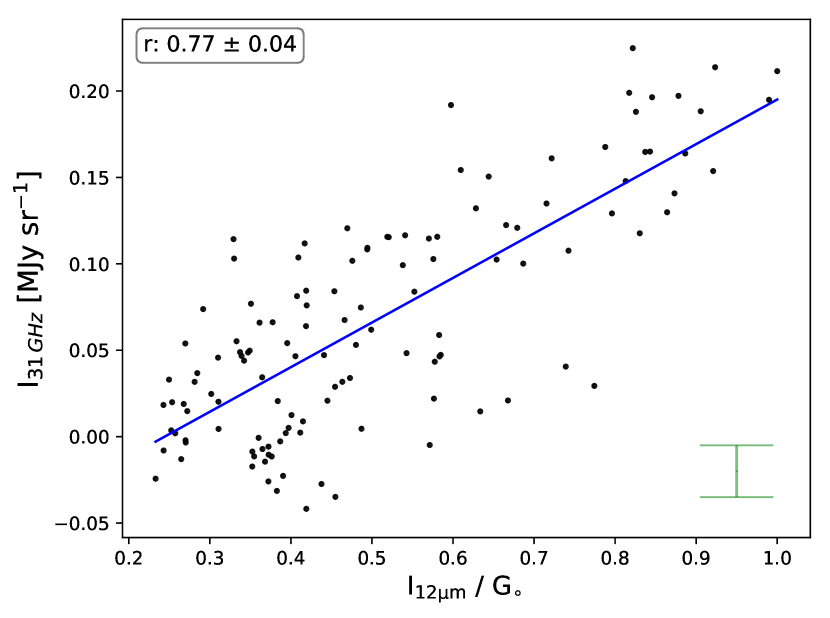
(a)

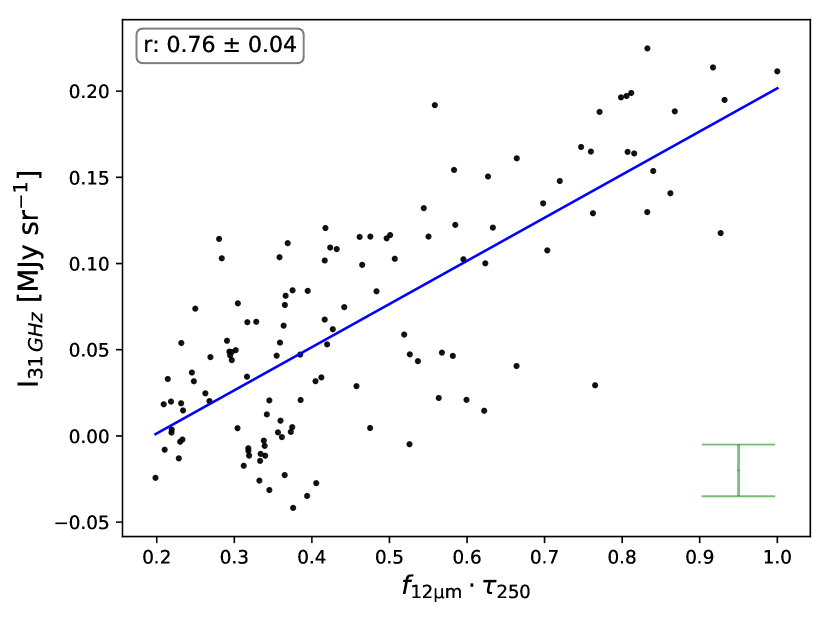
(b)

Figure 5: Linear correlations between the 31 GHz data and the column density proxies I${}_{12\,\mathrm{\upmu m}}$/G_∘ (5(a)) and f${}_{12\,\mathrm{\upmu m}}$ $\cdot$ $\tau_{250}$ (5(b)), in the plane of the sky. RMS error bars ($\sim$ 0.03 MJy sr^-1) are shown for the 31 GHz data. The column density proxies axis (x-axis) are normalized in both cases and their errors are negligible.

4.2 Pearson correlation analysis

Figure 5 shows the scatter plots using the 31 GHz data and column density proxies I${}_{\mathrm{12\,\upmu m}}/G_{0}$ and $f_{\mathrm{\,12\,\upmu m}}\,\cdot\,\tau_{250}$ in the plane of the sky. These scatter plots suggest a linear dependence between the CBI 2 data and each template, which justifies the use of the Pearson coefficient as a statistical measurement of the correlation. The Pearson correlation coefficient, $r$, provides a way to quantify and compare the degree of correlation between the 31 GHz signal and different templates, both in the $uv$-domain,

$$r_{uv}=\frac{\sum_{k}\omega_{k}\left(Vx_{k}-\overline{V}x\right)\left(Vy_{k}-\overline{V}y\right)}{\sqrt{\sum_{k}\omega_{k}\left(Vx_{k}-\overline{V}x\right)^{2}\sum_{k}\omega_{k}\left(Vy_{k}-\overline{V}y\right)^{2}}},$$ (10)

where $\omega_{k}$ is the weight for visibility datum $V_{k}$, and $\overline{V}x$ = $\sum_{k}\omega_{k}Vx_{k}/\sum_{k}\omega_{k}$ and $\overline{V}y$ = $\sum_{k}\omega_{k}Vy_{k}/\sum_{k}\omega_{k}$ are the weighted means of visibility data-sets $Vx$ and $Vy$, respectively; and in the sky-plane

$$r_{\mathrm{sky}}=\frac{\sum_{i}\left(x_{i}-\overline{x}\right)\left(y_{i}-\overline{y}\right)}{\sqrt{\sum_{i}\left(x_{i}-\overline{x}\right)^{2}\sum_{i}\left(y_{i}-\overline{y}\right)^{2}}},$$ (11)

where $\overline{x}$ and $\overline{y}$ are the mean values of data-sets $x$ and $y$, respectively.

The correlations in the $uv$-plane ($r_{\mathrm{uv}}$) are calculated for the entire visibility data-set. On the other hand, the sky-plane cross-correlations are taken inside an area equivalent to half the mosaic’s primary beam FWHM, shown as a dashed region in Figure 4(a). This helps us avoid noisy outliers and measure the correlation within the area of interest, which is the PDR. We also masked the PMN galaxy identified in Figure 1.

The uncertainties in $r_{\mathrm{sky}}$ were estimated with a Monte Carlo simulation. We added random Gaussian noise to the 31 GHz clean mosaic, before dividing by the mosaic attenuation map, with a dispersion given by the RMS noise of the 31 GHz clean mosaic. In each run of the simulations, the resulting 31 GHz intensity map is correlated with the corresponding template, and the final error in $r_{\mathrm{sky}}$ is the standard deviation of all the correlation coefficients. In the $uv$-plane, the $r_{\mathrm{uv}}$ errors are calculated under the same logic, but instead, we add random Gaussian noise to each visibility datum $V_{k}$ using a dispersion given by its weight $\omega_{k}=1/\sigma_{k}^{2}$, common to both the real and imaginary parts. We are interested in the relative variations of the Pearson coefficients between the templates, so any bias due to systematic errors will be the same for all the maps.

The resulting values for the correlations coefficients are listed in Table 5. We observe the same trends in both $r_{\mathrm{sky}}$ and $r_{\mathrm{uv}}$, although the sky-plane results show higher correlations. This difference is expected, as the sky correlations were extracted within 50 $\%$ of the primary beam area, while the $uv$-plane correlations used all of the visibilities, which are integrated quantities over the whole primary beams.

Figure 3(b) shows the cuts for the normalized radiance, $\tau_{250}$, and column density proxies, starting from star HD 147889 and passing through the 31 GHz emission peak (as shown by the arrow in Figure 2). Here, we see that the column density proxies of the small grains peak around the same location as the 31 GHz data. Note the shift of the IRAC 8$\upmu$m and WISE 12$\upmu$m profiles between Fig. 3(a) and their column density proxies in Fig. 3(b). It is also interesting to highlight that the location of the bump in the WISE 12$\upmu$m profile (at around 10 arcmin in Fig. 3(a)) matches the 31 GHz peak. This leads to a stronger correlation between both templates, which is also reflected in Fig. 3(b), where I${}_{\mathrm{12\,\upmu m}}/G_{0}$ and $f_{\mathrm{\,12\,\upmu m}}\,\cdot\,\tau_{250}$ are narrower and show a more similar profile to the 31 GHz data. As shown in Table 5, the best correlation is indeed with PAH column density proxy I${}_{\mathrm{12\,\upmu m}}/G_{0}$. The role of the WISE 3$\upmu$m map as a tracer for smaller PAHs will be discussed in Sec. 5.

Note that, in Figure 3(b), the radiance profile shows two peaks: one around 5 arcmin from HD 147889, which is related to hotter dust grains nearby the star, and a second one along the PDR but shifted $\sim$2 arcmin from the 31 GHz profile, which is related to a larger optical depth ($\tau_{250}$). The $\tau_{250}$ peak, which traces the concentration of big grains, is shifted towards the molecular cloud, matching the peak of $\mathrm{SPIRE}$ 250 $\upmu$m (Fig. 3(a)) at $\sim$13 arcmin. Table 5 shows that the $\tau_{250}$ map does not correlate with the 31 GHz map, while the correlation coefficient for the radiance template ($\mathcal{R}$) is moderate. Historically, sub-mm templates have been used to trace dust emission (Dickinson et al., 2018), but, in this case, the quantification of the sub-mm emission is better traced by the radiance in comparison with $\tau_{250}$ or the intensity at any given sub-mm frequency. This is consistent with the result by Hensley, Draine & Meisner (2016) where the radiance template is the best tracer for the AME.

Table 5: Pearson correlations between the 31 GHz data and different templates, for the plane of the sky ($r_{\mathrm{sky}}$) and the $uv$-plane ($r_{\mathrm{uv}}$).

Template	$r_{\mathrm{\,uv}}$	$r_{\mathrm{\,sky}}$
WISE 3	0.25 $\pm$ 0.01	0.61 $\pm$ 0.04
IRAC 8	0.26 $\pm$ 0.01	0.68 $\pm$ 0.04
WISE 12	0.29 $\pm$ 0.01	0.72 $\pm$ 0.04
WISE 22	0.15 $\pm$ 0.01	0.52 $\pm$ 0.04
MIPS 24	0.15 $\pm$ 0.01	0.51 $\pm$ 0.04
SPIRE 250	0.08 $\pm$ 0.01	0.40 $\pm$ 0.04
$\tau_{250}$	-0.04 $\pm$ 0.01	0.11 $\pm$ 0.04
$\mathcal{R}$/$\nu$	0.13 $\pm$ 0.01	0.51 $\pm$ 0.04
$f_{\mathrm{\,3\,\upmu m}}$	0.17 $\pm$ 0.01	0.23 $\pm$ 0.04
$f_{\mathrm{\,8\,\upmu m}}$	0.23 $\pm$ 0.01	0.32 $\pm$ 0.02
$f_{\mathrm{\,12\,\upmu m}}$	0.25 $\pm$ 0.01	0.37 $\pm$ 0.02
$f_{\mathrm{\,3\,\upmu m}}\,\cdot\,\tau_{250}$	0.27 $\pm$ 0.01	0.70 $\pm$ 0.04
$f_{\mathrm{\,8\,\upmu m}}\,\cdot\,\tau_{250}$	0.28 $\pm$ 0.01	0.59 $\pm$ 0.04
$f_{\mathrm{\,12\,\upmu m}}\,\cdot\,\tau_{250}$	0.34 $\pm$ 0.01	0.76 $\pm$ 0.04
I${}_{\mathrm{3\,\upmu m}}/G_{0}$	0.29 $\pm$ 0.01	0.71 $\pm$ 0.04
I${}_{\mathrm{8\,\upmu m}}/G_{0}$	0.26 $\pm$ 0.01	0.60 $\pm$ 0.04
I${}_{\mathrm{12\,\upmu m}}/G_{0}$	0.34 $\pm$ 0.01	0.77 $\pm$ 0.04

Table 6: Pearson coefficients for the original visibility data-set and the visibility data-set using uv-tapering for an equivalent angular resolution of 13.5 arcmin ($\sim$ 3 times the original CBI 2 angular resolution). We show the ratio between the Pearson coefficients of the two data-sets. In particular, we see that the dust radiance coefficient tends to increase the most at a lower equivalent angular resolution.

Template	$r_{\mathrm{\,uv}}$	$r_{\mathrm{\,uv-13.5\,^{\prime}}}$	Ratio
WISE 3	0.25 $\pm$ 0.01	0.32 $\pm$ 0.02	1.3 $\pm$ 0.1
IRAC 8	0.26 $\pm$ 0.01	0.35 $\pm$ 0.02	1.3 $\pm$ 0.1
WISE 12	0.29 $\pm$ 0.01	0.37 $\pm$ 0.02	1.3 $\pm$ 0.1
WISE 22	0.15 $\pm$ 0.01	0.20 $\pm$ 0.01	1.4 $\pm$ 0.1
MIPS 24	0.15 $\pm$ 0.01	0.20 $\pm$ 0.02	1.3 $\pm$ 0.2
SPIRE 250	0.08 $\pm$ 0.01	0.09 $\pm$ 0.01	1.1 $\pm$ 0.2
$\tau_{250}$	-0.04 $\pm$ 0.01	-0.06 $\pm$ 0.01	1.5 $\pm$ 0.4
$\mathcal{R}$/$\nu$	0.13 $\pm$ 0.01	0.20 $\pm$ 0.02	1.5 $\pm$ 0.2
$f_{\mathrm{\,3\,\upmu m}}$	0.17 $\pm$ 0.01	0.21 $\pm$ 0.02	1.2 $\pm$ 0.1
$f_{\mathrm{\,8\,\upmu m}}$	0.23 $\pm$ 0.01	0.29 $\pm$ 0.02	1.3 $\pm$ 0.1
$f_{\mathrm{\,12\,\upmu m}}$	0.25 $\pm$ 0.01	0.31 $\pm$ 0.02	1.2 $\pm$ 0.1
$f_{\mathrm{\,3\,\upmu m}}\,\cdot\,\tau_{250}$	0.27 $\pm$ 0.01	0.34 $\pm$ 0.01	1.3 $\pm$ 0.1
$f_{\mathrm{\,8\,\upmu m}}\,\cdot\,\tau_{250}$	0.28 $\pm$ 0.01	0.37 $\pm$ 0.03	1.3 $\pm$ 0.1
$f_{\mathrm{\,12\,\upmu m}}\,\cdot\,\tau_{250}$	0.34 $\pm$ 0.01	0.42 $\pm$ 0.03	1.2 $\pm$ 0.1
I${}_{\mathrm{3\,\upmu m}}/G_{0}$	0.29 $\pm$ 0.01	0.37 $\pm$ 0.03	1.3 $\pm$ 0.1
I${}_{\mathrm{8\,\upmu m}}/G_{0}$	0.26 $\pm$ 0.01	0.34 $\pm$ 0.03	1.3 $\pm$ 0.1
I${}_{\mathrm{12\,\upmu m}}/G_{0}$	0.34 $\pm$ 0.01	0.42 $\pm$ 0.03	1.2 $\pm$ 0.1

4.3 Correlation analysis as a function of angular resolution

The cross-correlations also depend on angular resolution. We repeated the correlations in the $uv$-plane for an equivalent angular resolution of 13.5 arcmin, closer to the approximate maximum recoverable scale ($\sim$ three times the CBI 2 synthesized beam). To do this, we applied a $uv$-taper by multiplying the visibility weights with a Gaussian, $W$ = $\exp{\left(-(u^{2}+v^{2})/t^{2}\right)}$. The results are presented in Table 6, where we also show the ratio between the Pearson coefficients of the original and the tapered data-set. These correlations show the highest increase for $\mathcal{R}/\nu$ and $\tau_{\mathrm{250}}$, but note that the correlation for $\tau_{\mathrm{250}}$ is very close to zero. We also calculated the correlations in the sky plane by smoothing the templates to angular resolutions of 9 and 13.5 arcmin and observed the same tendency: the Pearson coefficient of the dust radiance maps increases the most at lower angular resolutions, while the column density proxies tend to remain equal.

The fact that the radiance template shows the highest relative increase in its Pearson coefficient could explain the results obtained by Hensley, Draine & Meisner (2016), where their dust radiance template correlated the best with their AME template at an angular resolution of 1^∘. Based on their correlation results, they concluded that PAHs might not be responsible for the AME. This is not the case for our 4.5 arcmin maps, so we believe that PAHs cannot be ruled out as possible SD carriers. In this PDR, the 8 $\upmu$m and 12 $\upmu$m bands are dominated by PAHs (see e.g., Habart et al., 2003; Draine & Li, 2007; Compiègne et al., 2011), so the fact that we found a good correlation between these bands and the 31 GHz emission indicates that the PAHs might be important AME emitters.

Table 7: AME correlation slopes for $\rho$ Oph W between typical AME frequencies and dust templates. The $\tau_{353}$ map can be considered a better dust template as it traces the dust column density. We find that most of the $\rho$ Oph 31 GHz flux must be coming from $\rho$ Oph W.

Frequency [GHz]	Angular Resolution	Correlation slope	Units	Template	Reference
31	4.5 arcmin	15.5 $\pm$ 0.2	10${}^{6}\upmu$K	$\tau_{353}$	This work.
22.8	1∘	23.9 $\pm$ 2.3	10${}^{6}\upmu$K	$\tau_{353}$	Dickinson et al. (2018)
31	4.5 arcmin	2.18 $\pm$ 0.04	$\upmu$K / (MJy sr-1)	100 $\upmu$m (IRIS)	This work.
22.8	1∘	8.3 $\pm$ 1.1	$\upmu$K / (MJy sr-1)	100 $\upmu$m (IRIS)	Dickinson et al. (2018)

4.4 AME correlation slopes

Typically, AME emissivities have been quantified with correlation slopes in terms of IR emission (e.g. I${}_{\mathrm{30\,GHz}}$ / I${}_{\mathrm{100\,\upmu m}}$) or using an optical depth map (I${}_{\mathrm{30\,GHz}}$ / $\tau_{\mathrm{353\,GHz}}$) (see Dickinson et al., 2018). We calculated the correlation slope between our 31 GHz data, and $\tau_{353}$ and IRIS 100 $\upmu$m. For this, we measured the mean emission within the PDR filament using intensities larger than 15$\sigma$ (as the contour defined in Fig.1) in the primary beam corrected clean map. The original angular resolutions for the $\tau_{353}$ and IRIS 100 $\upmu$m maps (5 and 4.3 arcmin, respectively) are very similar to CBI 2’s angular resolution of 4.5 arcmin. In Table 7 we list the values for the AME correlation slopes. We also show the correlation slopes measured with the same templates by Dickinson et al. (2018), at an angular resolution of 1^∘. We find that a large fraction of the AME correlation slope measured in $\rho$ Oph on scales of 1^∘ must be coming from the $\rho$ Oph W PDR. This is especially evident when using the $\tau_{353}$ map, where the AME correlation slope of the 4.5 arcmin $\rho$ Oph W PDR observations is $\sim$65$\%$ of the AME correlation slope of the 1 ^∘ $\rho$ Oph observations. $\rho$ Oph W shows the highest AME emissivity in terms of the $\tau_{353}$ map, which is considered as a very reliable dust template as it traces the dust column density (Dickinson et al., 2018). These emissivities are about a factor 2-3 higher than other values measured at high Galactic latitudes and also in Perseus, the brightest AME source in the sky according to Planck Collaboration et al. (2011). A possible explanation for the larger slope in $\rho$ Oph W could be found in the finer linear resolution in this work, of $\sim$0.2 pc, compared to $\sim$2.3 pc in Planck Collaboration et al. (2011). The fact that $\rho$ Oph is closer to us means that we can resolve the AME from the PDR. When integrated in the telescope beam (e.g. Planck analysis over 1^∘ scales), there is proportionally a larger amount of AME coming from the high density and excited PDR compared to the emission from the regions that have lower emissivities, i.e. AME from the denser cores, or from the more diffuse gas.

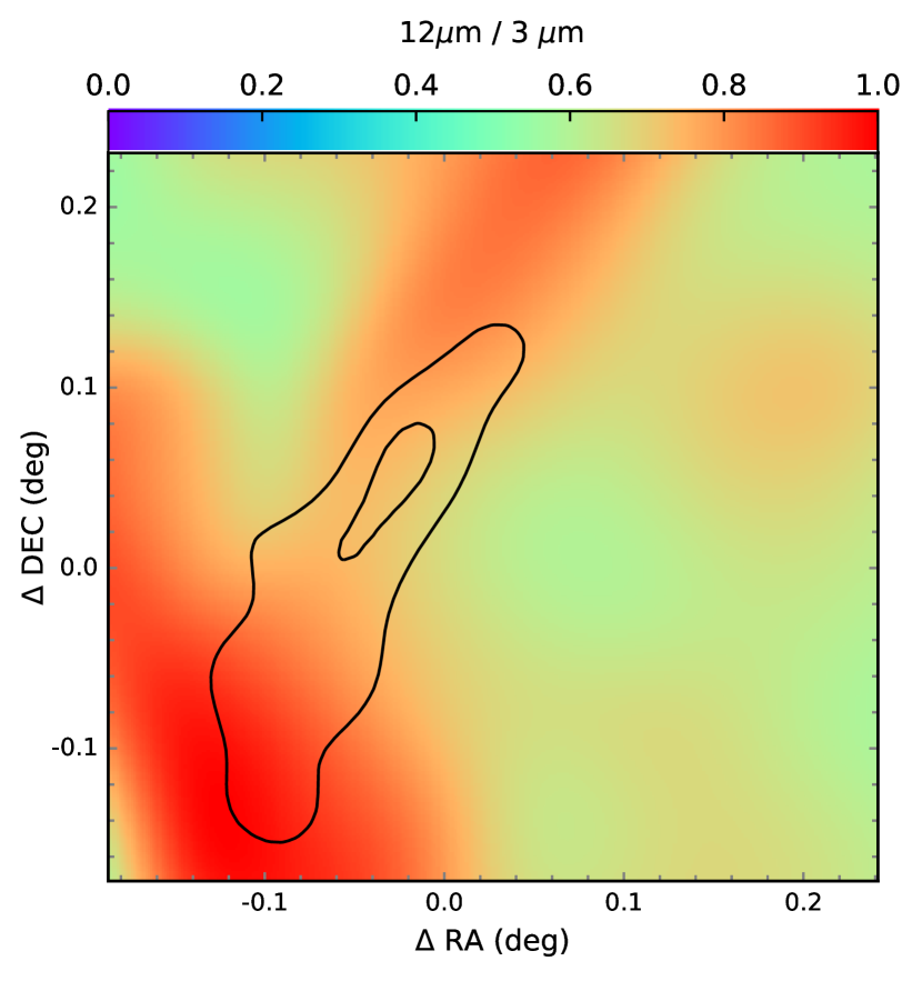
(a)

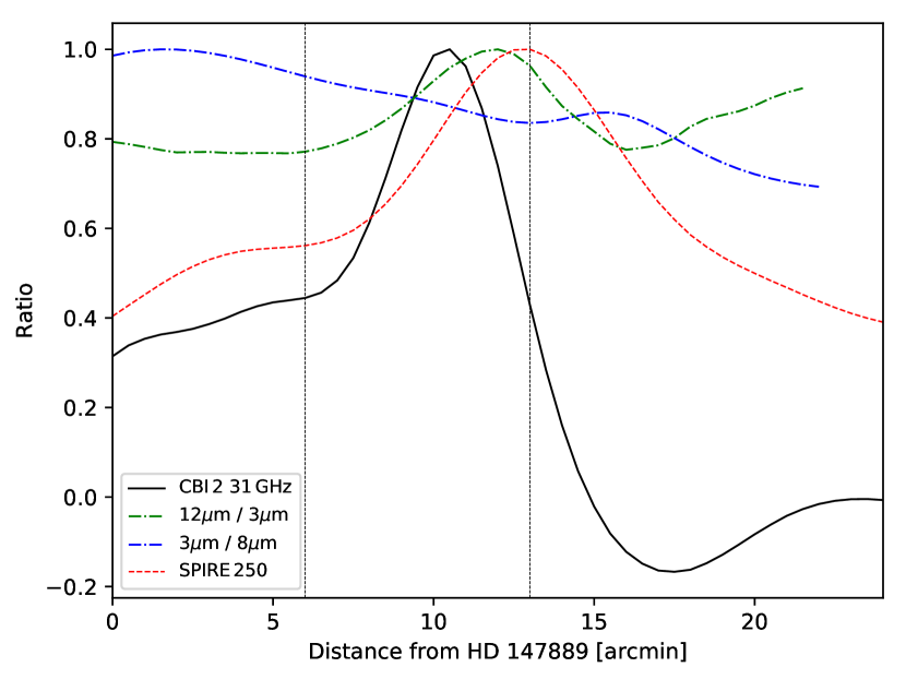
(b)

Figure 6: 6(a): Normalized 12 $\upmu$m / 3 $\upmu$m ratio in the $\rho$ Oph W PDR. 6(b): normalized emission profiles vs. distance to ionizing star HD 147889 for the 12 $\upmu$m / 3 $\upmu$m and 3 $\upmu$m / 8 $\upmu$m ratios in comparison to the 31 GHz and 250 $\upmu$m emission. The profile cut corresponds to the dashed arrow in Fig. 2 and the black vertical lines define the PDR.

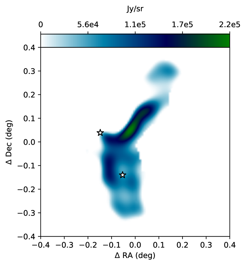
(a) gpu-uvmem model map

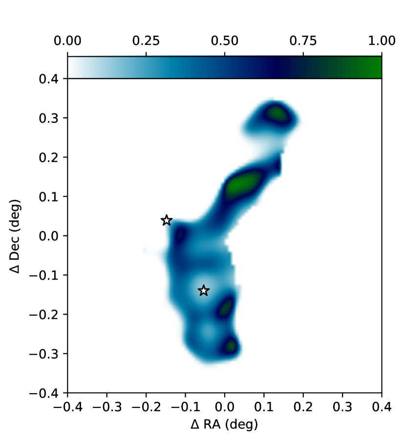
(b) gpu-uvmem $\hat{j_{\nu}}_{\,\mathrm{proxy}}$ map

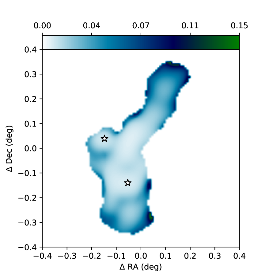
(c) $\hat{j_{\nu}}_{\,\mathrm{proxy}}$ noise map

Figure 7: 7(a): CBI 2 31 GHz gpu-uvmem model image. 7(b): normalized $\hat{j_{\nu}}_{\,\mathrm{proxy}}$ map (with a peak of 2.19 $\pm$ 0.04, in arbitrary units) and 7(c): $\hat{j_{\nu}}_{\,\mathrm{proxy}}$ - normalized noise map (the scale corresponds to that of Fig. 7(b)). We used a mask around HD 147889 in order to avoid the bulk of the free-free emission. The observed blob towards the northern part of the filament is detected at 3$\sigma$ over the noise in the CBI 2 clean map and could be the continuation of the PDR emission (no catalogued source was identified in that position).

4.5 Spectral index

The wide frequency coverage of the CBI 2 correlator, between 26 GHz and 36 GHz, may place constraints on the spectral properties of the 31 GHz signal. We split the visibilities ($V$) in two sub-sets: one for the low frequency channels (6-10) centered at 28.5 GHz, and one for the high frequency channels (1-5) centered at 33.5 GHz. We then calculated the correlation slopes (a^High, a^Low) between the two sub-sets and the mock visibilities for I${}_{\mathrm{12\,\upmu m}}/G_{0}$ (the best correlated proxy), following:

$$V_{31\,\mathrm{GHz}}^{\mathrm{High/Low}}=\mathrm{a}^{\mathrm{High/Low}}\,\,V_{12\,\upmu\mathrm{m}/G_{0}}.$$ (12)

Note that $\log{(\mathrm{a}^{\mathrm{High}}/\mathrm{a}^{\mathrm{Low}})}$ is proportional to the spectral index $\alpha$. We obtained a spectral index of $\alpha$ = 0.05 $\pm$ 0.08, which indicates a flat spectrum. However, we must also take into account the difficulty of obtaining a reliable spectral index due to any possible calibration and systematic errors. The spectral index measured between the low and high frequency channel is nonetheless consistent with the shape of the $\rho$ Oph spectrum in Planck Collaboration et al. (2011).

5 Qualitative analysis of the PAH sizes

The results in Table 5 show that column density proxies of PAH tracers at 3 $\upmu$m, 8 $\upmu$m and 12 $\upmu$m correlate the best with the 31 GHz emission. Note that, in particular, the 3 $\upmu$m band is dominated by the smallest PAHs (sizes $\sim$0.4 nm), which are the most prone to destruction by UV radiation, while the 8 $\upmu$m and 12 $\upmu$m bands, in comparison, are dominated by bigger PAHs. Given this, a good tracer of the PAH sizes is the 12 $\upmu$m / 3 $\upmu$m ratio map (Allamandola, Tielens & Barker, 1985; Ricca et al., 2012; Croiset et al., 2016). To construct it, we removed the point sources in the WISE 3 $\upmu$m map, and smoothed both the WISE 12 $\upmu$m and 3 $\upmu$m maps to CBI 2’s angular resolution. In Fig. 6(a) we show the 4.5 arcmin map for the 12 $\upmu$m / 3 $\upmu$m ratio, along with the 31 GHz contours (same contours as in Fig. 1). At this angular resolution, it is interesting to note the increment of the ratio in the transition between the PDR and the molecular cloud to the East in Fig. 6(a). This is also seen in Fig. 6(b), where we show the normalized emission profiles for the cut in Fig. 2 vs. the distance to the ionizing star HD 147889. Here, the minimum of the 12 $\upmu$m / 3 $\upmu$m ratio is aligned with the PDR surface (defined by the first black vertical line, $\sim$6 arcmin in Fig. 6(b)), while the peak of the ratio occurs at the transition between the PDR and the molecular cloud (defined by the second black vertical line, $\sim$14 arcmin in Fig. 6(b)). This peak might be an indication that the PAHs size increases in the PDR towards the molecular cloud.

The 3 $\upmu$m / 8 $\upmu$m ratio map can also give us an indication of the contribution of the smallest PAHs. We calculated the plane of the sky correlation between the 3 $\upmu$m / 8 $\upmu$m ratio and the 31 GHz emission, and obtained a Pearson coefficient of $r_{\mathrm{sky}}$ = $-$0.21 $\pm$ 0.03. The low value of the anti-correlation indicates that the smallest grains do not necessarily correlate better with the 31 GHz map, as it can also be seen in Table 5, where the correlation in WISE 3 is not better than with IRAC 8. Fig. 6(b) also shows the normalized profile for the 3 $\upmu$m / 8 $\upmu$m ratio. The behaviour of this template is similar to the 12 $\upmu$m / 3 $\upmu$m map, but shifted towards the interior of the molecular cloud. Overall, these ratios reveal a factor of $\sim$1.5 variation in the size of the emitting PAHs throughout the $\rho$ Oph W PDR.

6 Emissivity Variations

In our correlation analysis (Sec. 4) we found that the 31 GHz map correlates best with I${}_{\mathrm{12\,\upmu m}}/G_{0}$, a template for the PAH column density. Also, we note that there is significant scatter about the linear cross-correlations between the 31 GHz emission and the PAH column density proxies, as shown in Fig. 5. Motivated by this, we study the possibility that this scatter is produced by SD emissivity variations along the PDR.

In order to assess the extent to which the physical mechanisms leading to the 31 GHz emission depend on the local environment, we tested for the hypothesis that the emergent 31 GHz intensity is only proportional to the column of the emitters, i.e. $N_{\mathrm{PAH}}$. We construct a proxy that will let us measure any emissivity variation in the PDR as in Casassus et al. (2008), and define the 31 GHz emissivity per SD emitter (i.e. PAHs in our hypothesis), $\hat{j_{\nu}}$, which should be proportional to the SD emissivity per H-nucleus for a fixed grain population:

$$\hat{j_{\nu}}\equiv\frac{I_{\nu}(31\mathrm{GHz})}{N_{\mathrm{PAH}}}\propto j_{\nu}\equiv\frac{I_{\nu}}{N_{H}}.$$ (13)

Using Eq. 6 we can propose a proxy for $\hat{j_{\nu}}$:

$${\hat{j_{\nu}}}_{\,\mathrm{proxy}}\equiv\frac{I_{\nu}(31\mathrm{GHz})}{I_{\mathrm{12\,\upmu m}}/G_{0}}.$$ (14)

The gpu-uvmem model images for $I^{\mathrm{uvmem}}_{\nu}(31\mathrm{GHz})$ and $I^{\mathrm{uvmem}}_{\mathrm{12\,\upmu m}}/G_{0}$ provide a finer angular resolution than the clean mosaic, and may pick up larger variations in emissivity. Figure 7 shows $I^{\mathrm{uvmem}}_{\nu}(31\mathrm{GHz})$ (Fig. 7(a)), as well as the normalized $\hat{j_{\nu}}_{\,\mathrm{proxy}}$ map defined in Eq. 14 (Fig. 7(b)), along with its noise map (Fig. 7(c)). As explained in Section 3, the bulk of the free-free emission is located around HD 147889. Given this, we masked a region with a radius of 6 arcmin around HD 147889 in the gpu-uvmem maps, in order to quantify only the SD component using $\hat{j_{\nu}}_{\,\mathrm{proxy}}$. Note that the $\hat{j_{\nu}}_{\,\mathrm{proxy}}$ map (Fig. 7(b)) shows variations throughout the region, with a peak that matches the peak at 31 GHz in the $\rho$ Oph W PDR.

Table 8: Emissivities variations in $\rho$ Oph measured with the $\hat{j_{\nu}}_{\,\mathrm{proxy}}$ map.

Ratio		R
$\mathrm{S/N}_{\mathrm{\,Peak\,at\,\,3\sigma}}$a		25.6
$\hat{j_{\nu}}_{\mathrm{proxy-\,Peak}}$ / $\hat{j_{\nu}}_{\mathrm{proxy-\,S1}}$b		22.8 $\pm$ 5.2
$\hat{j_{\nu}}_{\mathrm{proxy-\,Peak}}$ / $\hat{j_{\nu}}_{\mathrm{proxy-\,SR3}}$c		6.2 $\pm$ 0.3

^a Ratio between the emissivity peak and its 3$\sigma$ noise.
^b Ratio between the peak and at the location of S1.
^c Ratio between the peak and at the location of SR3.

In Table 8 we list $\hat{j_{\nu}}_{\,\mathrm{proxy}}$ variations for different locations in the region. We found that the $\hat{j_{\nu}}_{\,\mathrm{proxy}}$ map has a peak that is 25 times higher than the 3$\sigma$ noise. We repeated this calculation on a clean $\hat{j_{\nu}}_{\,\mathrm{proxy}}$ map and found an emissivity peak 10 times stronger than its 3$\sigma$ noise. This difference is expected, as the gpu-uvmem map resolves much better the CBI 2 morphology.

Interestingly, the emissivity variation between the $\hat{j_{\nu}}_{\,\mathrm{proxy}}$ peak and the location of S1 is 22.8, very close to the strongest variation in $\rho$ Oph W at 3$\sigma$. The fact that there is no significant 31 GHz emission originating at S1 (as seen in Figures 1 and 2) implies that the radio-emission mechanism is enhanced by the local conditions in the PDR, otherwise, we would see higher levels of 31 GHz emission near S1, given its large column of small grains (i.e. PAHs) (Casassus et al., 2008).

The nature of the SD emissivity variations in $\rho$ Oph may rely on various scenarios. SD models predict peak frequencies in the range 50-90 GHz for the typical environmental conditions of a PDR (e.g. Draine & Lazarian, 1998a; Ysard, Juvela & Verstraete, 2011; Hensley & Draine, 2017a). However, only one reported observation of the California nebula is consistent with a SD spectrum with a (50 $\pm$ 17) GHz peak (Planck Collaboration et al., 2014c). It is clear that the frequency of the SD spectrum must be changing due to environmental conditions across the PDR. In this case, the observed emissivity variations could be associated with a shift in the peak frequency. Nevertheless, the analysis in this work is based on the assumption that the 31 GHz emission maps the AME.

A tentative explanation for the local emissivity boost, in the SD paradigm, could be that the main spin-up mechanism in $\rho$ Oph W are ion collisions (Draine & Lazarian, 1998b). The electromagnetic coupling between passing C⁺ ions and the grain dipole moment impart torques on the grain. As the rotational excitation by ions is more effective for charged grains (Hensley & Draine, 2017a), a possible explanation could be that the PDR is hosting preferentially charged PAHs spun-up by C⁺. As observed in Fig. 7, the fainter signal from S1 and SR3 in the radio maps of $\rho$ Oph could then be naturally explained by the fact that these stars are too cold to create conspicuous Cii regions (Casassus et al., 2008). In addition to the rotational excitation of charged grains, we could also add the effect of a possible changing penetration of the ISRF through the PDR due to the morphology of the cloud. The variations in the ISRF intensity affect the grain size distribution and, most likely, their dipole moment, and these factors can produce considerable changes in the SD emissivity (Hoang, Lazarian & Draine, 2011). Thus, further analysis of the PDR spectrum at different radio-frequencies is required to calculate its physical parameters and understand the causes of the detected SD emissivity variations.

7 Conclusions

We report 31 GHz observations from CBI 2 of the $\rho$ Oph W PDR, at an angular resolution of 4.5 arcmin. The emission runs along the PDR exposed to the ionizing star HD 147889. Interestingly, there is no significant 31 GHz emission from S1, the brightest IR nebula in the complex.

To understand the nature of the 31 GHz emission, we calculated the correlations of the CBI 2 data with different IR templates, with PAHs column density proxies, and with dust radiance and optical depth templates. We show that the 31 GHz emission is related to the local PAH column density. The best correlation was found when using the 12 $\upmu$m PAH column density proxy and it is significantly better than when using the 8 $\upmu$m and 3 $\upmu$m PAH column density proxies.

We also measured the correlations at different angular resolutions and found that the dust radiance correlation is better at lower angular resolution. This shows that the effect of angular resolution must be considered when interpreting morphological correlations, implying in this case that PAH’s cannot be ruled out as spinning dust carriers, as previous studies at lower angular resolutions have suggested. Additionally, we calculated a spectral index of $\alpha$ = 0.05 $\pm$ 0.08, between 28.5 GHz and 33.5 GHz, that is consistent with the flat spectrum previously reported on this region. By using a 12 $\upmu$m / 3 $\upmu$m ratio map, we measured an increase of the PAH size in the transition between the PDR and the molecular cloud.

Motivated by the intrinsic scatter in the correlation plots, we constructed a proxy for the 31 GHz emissivity per spinning dust emitter so as to quantify its variations. Using a gpu-uvmem model of the 31 GHz emission, we found that the spinning dust emissivity peak over the PDR is, at least, 25 times greater over the noise, at 3$\sigma$, and 23 times greater than at the location of star S1, also at 3$\sigma$.

The spinning dust emissivity boost in $\rho$ Oph W appears to be dominated by local conditions in the PDR. Based on the fainter 31 GHz signal from stars S1 and SR3, possible explanations are environmental ions or a changing grain population. In the framework of the spinning dust interpretation, these emissivity variations may hold the key to identify the dominant grain spin-up mechanisms. Further multi-frequency radio analysis of the PDR spectrum is needed in order to better understand the conditions that give rise to spinning dust.

References

- Ali-Haïmoud, Hirata & Dickinson (2009) Ali-Haïmoud Y., Hirata C. M., Dickinson C., 2009, MNRAS, 395, 1055
- Allamandola, Tielens & Barker (1985) Allamandola L. J., Tielens A. G. G. M., Barker J. R., 1985, ApJ, 290, L25
- Ami Consortium et al. (2009) Ami Consortium et al., 2009, MNRAS, 394, L46
- André et al. (2010) André P. et al., 2010, A&A, 518, L102
- Battistelli et al. (2015) Battistelli E. S. et al., 2015, ApJ, 801, 111
- Battistelli et al. (2019) Battistelli E. S. et al., 2019, ApJ, 877, L31
- Bennett et al. (2013) Bennett C. L. et al., 2013, ApJS, 208, 20
- Bondar (2012) Bondar A., 2012, MNRAS, 423, 725
- Cárcamo et al. (2018) Cárcamo M., Román P. E., Casassus S., Moral V., Rannou F. R., 2018, Astronomy and Computing, 22, 16
- Casassus et al. (2006) Casassus S., Cabrera G. F., Förster F., Pearson T. J., Readhead A. C. S., Dickinson C., 2006, ApJ, 639, 951
- Casassus et al. (2008) Casassus S. et al., 2008, MNRAS, 391, 1075
- Castellanos et al. (2011) Castellanos P. et al., 2011, MNRAS, 411, 1137
- Compiègne et al. (2011) Compiègne M. et al., 2011, A&A, 525, A103
- Condon et al. (1998) Condon J. J., Cotton W. D., Greisen E. W., Yin Q. F., Perley R. A., Taylor G. B., Broderick J. J., 1998, AJ, 115, 1693
- Croiset et al. (2016) Croiset B. A., Candian A., Berné O., Tielens A. G. G. M., 2016, A&A, 590, A26
- Davies et al. (2006) Davies R. D., Dickinson C., Banday A. J., Jaffe T. R., Górski K. M., Davis R. J., 2006, MNRAS, 370, 1125
- Dickinson et al. (2018) Dickinson C. et al., 2018, New Astron. Rev., 80, 1
- Dickinson et al. (2009) Dickinson C. et al., 2009, ApJ, 690, 1585
- Dickinson et al. (2007) Dickinson C., Davies R. D., Bronfman L., Casassus S., Davis R. J., Pearson T. J., Readhead A. C. S., Wilkinson P. N., 2007, MNRAS, 379, 297
- Draine & Lazarian (1998a) Draine B. T., Lazarian A., 1998a, ApJ, 494, L19+
- Draine & Lazarian (1998b) Draine B. T., Lazarian A., 1998b, ApJ, 508, 157
- Draine & Li (2007) Draine B. T., Li A., 2007, ApJ, 657, 810
- Erickson (1957) Erickson W. C., 1957, ApJ, 126, 480
- Fazio et al. (2004) Fazio G. G. et al., 2004, ApJS, 154, 10
- Finkbeiner (2004) Finkbeiner D. P., 2004, ApJ, 614, 186
- Gaia Collaboration et al. (2018) Gaia Collaboration et al., 2018, A&A, 616, A1
- Galliano (2018) Galliano F., 2018, MNRAS, 476, 1445
- Génova-Santos et al. (2015) Génova-Santos R. et al., 2015, MNRAS, 452, 4169
- Griffin et al. (2010) Griffin M. J. et al., 2010, A&A, 518, L3
- Griffith et al. (1994) Griffith M. R., Wright A. E., Burke B. F., Ekers R. D., 1994, The Astrophysical Journal Supplement Series, 90, 179
- Habart et al. (2003) Habart E., Boulanger F., Verstraete L., Pineau des Forêts G., Falgarone E., Abergel A., 2003, A&A, 397, 623
- Healey et al. (2007) Healey S. E., Romani R. W., Taylor G. B., Sadler E. M., Ricci R., Murphy T., Ulvestad J. S., Winn J. N., 2007, The Astrophysical Journal Supplement Series, 171, 61
- Hensley, Murphy & Staguhn (2015) Hensley B., Murphy E., Staguhn J., 2015, MNRAS, 449, 809
- Hensley & Draine (2017a) Hensley B. S., Draine B. T., 2017a, ApJ, 836, 179
- Hensley & Draine (2017b) Hensley B. S., Draine B. T., 2017b, ApJ, 834, 134
- Hensley, Draine & Meisner (2016) Hensley B. S., Draine B. T., Meisner A. M., 2016, ApJ, 827, 45
- Hoang, Lazarian & Draine (2011) Hoang T., Lazarian A., Draine B. T., 2011, ApJ, 741, 87
- Hoang, Vinh & Quynh Lan (2016) Hoang T., Vinh N.-A., Quynh Lan N., 2016, ApJ, 824, 18
- Houk & Smith-Moore (1988) Houk N., Smith-Moore M., 1988, Michigan Catalogue of Two-dimensional Spectral Types for the HD Stars. Volume 4, Declinations -26.0 to -12.0.
- Kogut et al. (1996) Kogut A., Banday A. J., Bennett C. L., Gorski K. M., Hinshaw G., Reach W. T., 1996, ApJ, 460, 1
- Ladjelate et al. (2020) Ladjelate B. et al., 2020, arXiv e-prints, arXiv:2001.11036
- Leitch et al. (1997) Leitch E. M., Readhead A. C. S., Pearson T. J., Myers S. T., 1997, ApJ, 486, L23+
- Liseau et al. (1999) Liseau R. et al., 1999, A&A, 344, 342
- McMullin et al. (2007) McMullin J. P., Waters B., Schiebel D., Young W., Golap K., 2007, in Astronomical Society of the Pacific Conference Series, Vol. 376, Astronomical Data Analysis Software and Systems XVI, Shaw R. A., Hill F., Bell D. J., eds., p. 127
- Meisner & Finkbeiner (2014) Meisner A. M., Finkbeiner D. P., 2014, ApJ, 781, 5
- Murphy et al. (2010a) Murphy E. J. et al., 2010a, ApJ, 709, L108
- Murphy et al. (2018) Murphy E. J., Linden S. T., Dong D., Hensley B. S., Momjian E., Helou G., Evans A. S., 2018, ApJ, 862, 20
- Murphy et al. (2010b) Murphy T. et al., 2010b, MNRAS, 402, 2403
- Nolan et al. (2012) Nolan P. L. et al., 2012, ApJS, 199, 31
- Padin et al. (2002) Padin S. et al., 2002, PASP, 114, 83
- Pearson et al. (2003) Pearson T. J. et al., 2003, ApJ, 591, 556
- Pilbratt et al. (2010) Pilbratt G. L. et al., 2010, A&A, 518, L1
- Pilleri et al. (2012) Pilleri P., Montillaud J., Berné O., Joblin C., 2012, A&A, 542, A69
- Planck Collaboration et al. (2014a) Planck Collaboration et al., 2014a, A&A, 571, A11
- Planck Collaboration et al. (2013) Planck Collaboration et al., 2013, A&A, 557, A53
- Planck Collaboration et al. (2014b) Planck Collaboration et al., 2014b, A&A, 571, A12
- Planck Collaboration et al. (2011) Planck Collaboration et al., 2011, A&A, 536, A20
- Planck Collaboration et al. (2015) Planck Collaboration et al., 2015, A&A, 582, A28
- Planck Collaboration et al. (2014c) Planck Collaboration et al., 2014c, A&A, 565, A103
- Readhead et al. (2004a) Readhead A. C. S. et al., 2004a, ApJ, 609, 498
- Readhead et al. (2004b) Readhead A. C. S. et al., 2004b, Science, 306, 836
- Ricca et al. (2012) Ricca A., Bauschlicher, Charles W. J., Boersma C., Tielens A. G. G. M., Allamand ola L. J., 2012, ApJ, 754, 75
- Rieke et al. (2004) Rieke G. H. et al., 2004, ApJS, 154, 25
- Scaife et al. (2010a) Scaife A. M. M. et al., 2010a, MNRAS, 403, L46
- Scaife et al. (2010b) Scaife A. M. M. et al., 2010b, MNRAS, 406, L45
- Sellgren et al. (1985) Sellgren K., Allamandola L. J., Bregman J. D., Werner M. W., Wooden D. H., 1985, ApJ, 299, 416
- Sowards-Emmerd et al. (2004) Sowards-Emmerd D., Romani R. W., Michelson P. F., Ulvestad J. S., 2004, ApJ, 609, 564
- Taylor et al. (2011) Taylor A. C. et al., 2011, MNRAS, 418, 2720
- Tibbs et al. (2011) Tibbs C. T. et al., 2011, MNRAS, 418, 1889
- Tibbs et al. (2016) Tibbs C. T. et al., 2016, MNRAS, 456, 2290
- Tibbs et al. (2013) Tibbs C. T., Scaife A. M. M., Dickinson C., Paladini R., Davies R. D., Davis R. J., Grainge K. J. B., Watson R. A., 2013, ApJ, 768, 98
- Tielens (2008) Tielens A. G. G. M., 2008, ARA&A, 46, 289
- Vidal et al. (2011) Vidal M. et al., 2011, MNRAS, 414, 2424
- Vidal et al. (2020) Vidal M., Dickinson C., Harper S. E., Casassus S., Witt A. N., 2020, MNRAS, 495, 1122
- Watson et al. (2005) Watson R. A., Rebolo R., Rubiño-Martín J. A., Hildebrandt S., Gutiérrez C. M., Fernández-Cerezo S., Hoyland R. J., Battistelli E. S., 2005, ApJ, 624, L89
- Wright et al. (2010) Wright E. L. et al., 2010, AJ, 140, 1868
- Ysard, Juvela & Verstraete (2011) Ysard N., Juvela M., Verstraete L., 2011, A&A, 535, A89
- Ysard, Miville-Deschênes & Verstraete (2010) Ysard N., Miville-Deschênes M. A., Verstraete L., 2010, A&A, 509, L1