Topological Spin Liquids: Robustness under perturbations

Abstract

We study the robustness of the paradigmatic kagome Resonating Valence Bond (RVB) spin liquid and its orthogonal version, the quantum dimer model. The non-orthogonality of singlets in the RVB model and the induced finite length scale not only makes it difficult to analyze, but can also significantly affect its physics, such as how much noise resilience it exhibits. Surprisingly, we find that this is not the case: The amount of perturbations which the RVB spin liquid can tolerate is not affected by the finite correlation length, making the dimer model a viable model for studying RVB physics under perturbations. Remarkably, we find that this is a universal phenomenon protected by symmetries: First, the dominant correlations in the RVB are spinon correlations, making the state robust against doping with visons. Second, reflection symmetry stabilizes the spin liquid against doping with spinons, by forbidding mixing of the initially dominant correlations with those which lead to the breakdown of topological order.

I Introduction

Topological spin liquids (TSL) are exotic phases of matter where a system does not order magnetically despite strong antiferromagnetic interactions, but rather topologically, i.e. in its global entanglement. The interest in these systems stems from their unconventional properties, such as anyonic excitations with fractional charge and non-trivial statistics, and a ground space protected by its global entanglement [1, 2, 3]. However, TSLs are notoriously difficult to identify, both in theory and in experiment, as candidate systems often exhibit close competition between a number of different phases. In order to robustly realize these phases, it is therefore essential to understand how sensitively they react to perturbations which can induce a breakdown of topological order.

The paradigmatic example of a spin liquid is the Resonating Valence Bond (RVB) wavefunction on the kagome lattice, which consists of a “resonating” superposition of all possible ways to cover the lattice with nearest-neighbor singlets [4, 5]. It forms a physically motivated low-energy ansatz for Heisenberg-type models, and appears as the exact ground state of a local model with topological order [6, 7]. However, the non-orthogonality of different singlet configurations makes RVB models hard to analyze. To mitigate this difficulty, dimer models have been studied instead, where different singlet configurations are taken to be orthogonal [8]. The resulting kagome dimer model is an RG fixed point and thus significantly easier to analyze [9]. However, it is unclear to what extent results derived for the dimer model still apply to the RVB state, where the non-orthogonality of singlets induces a finite correlation length, making it doubtful whether the robustness of the RVB state can be understood from studies performed on the dimer model.

In this paper, we study and compare how sensitively the RVB spin liquid and the quantum dimer model react to noise, and which level of perturbations they can tolerate before their topological order breaks down. We consider both magnetic fields and lattice anisotropies, corresponding to doping with the two elementary topological excitations: spinons and visons. We find, rather surprisingly, that in both cases the RVB model exhibits essentially the same stability as the dimer model despite its non-zero correlation length. This suggests that the dimer model is more accurate in modeling spin liquid physics under perturbations than one might have naively assumed.

To understand the mechanism behind this unexpected result and its range of applicability, we microscopically analyze the structure of anyon correlations using tensor networks. Diverging anyon correlations indicate a closing gap, driving a phase transition through anyon condensation; the finite spinon correlations in the RVB would thus indeed suggest a decreased robustness. However, as our analysis reveals, there is a universal mechanism underlying the surprising robustness of the RVB model: It arises from symmetries which protect specific correlations, and is thus independent of the specific perturbation but rather a universal feature of the RVB spin liquid.

Concretely, we find that the non-orthogonality of singlets induces dominant spinon correlations without a separate vison correlation scale; since vison doping only increases the latter, the response is unaffected by the spinon length scale. The reason for the robustness to spinon doping is more subtle; we assess it through a combination of analytical and numerical study. It reveals that the spinon correlations exhibit a two-fold degeneracy in addition to the spin doublet. It originates in the two different ways to construct spinon correlations – either through the overlap of two states with one spinon each, separated by some distance $\ell$, or through the overlap of the original doped RVB with a state with two additional spinons placed at a separation $\ell$. We show that the reflection symmetry of the RVB rules out any correlation between spinons of opposite spin, also at finite doping. This, together with the symmetry of these overlaps under ket$\leftrightarrow$bra exchange, implies that the 4-fold multiplet splits under doping into sectors labelled by (i) their spin $\pm\tfrac{1}{2}$ and (ii) a fixed relative phase $\pm 1$ between the spinon at either position being in the ket or bra vector in the overlap, respectively. As we show, this $\pm 1$ phase label is protected by the reflection symmetry of the lattice and thus stable to perturbations which respect that symmetry. We find that the correlations which are initially enhanced by magnetic fields and those which drive the phase transition live in different sectors which are protected by the lattice symmetry; that explains why the presence of initial spinon correlations in the RVB state has no effect on its robustness to magnetic fields.

II RVB and dimer model

The RVB state is constructed as follows. First, we define a dimer covering as a full covering of the lattice with pairs of adjacent vertices, termed dimers (blue in Fig. 1a); we denote dimer coverings by $D$, and the set of all coverings (with PBC) by $\mathcal{D}$. Next, replace each dimer by a singlet $\left|\sigma\right\rangle=\tfrac{1}{\sqrt{2}}(\left|\uparrow\downarrow\right\rangle-\left|\downarrow\uparrow\right\rangle)$ (with counterclockwise orientation around triangles), we call the resulting state $\left|\bm{\sigma}(D)\right\rangle$. The RVB wavefunction is then $\left|\mathrm{RVB}\right\rangle=\sum_{D\in\mathcal{D}}\left|\bm{\sigma}(D)\right\rangle$. In studying the physics of RVB wavefunctions, so-called dimer models $\left|\mathrm{dimer}\right\rangle=\sum_{D\in\mathcal{D}}\left|D\right\rangle$ are frequently used, where the $\{\left|D\right\rangle\}_{D\in\mathcal{D}}$ define an orthonormal basis [8]. Replacing singlet configurations by orthogonal dimer configurations makes these models easier to analyze, but can also affect their physics. One way to explicitly construct a dimer representation is to start from the RVB wavefunction and attach arrows to each vertex [10] which for any dimer configuration $D$ point into the triangle where the adjacent dimer lies, Fig. 1a. These arrows can be treated as quantum degrees of freedom or “arrow qubits” with basis states $\{\left|a_{\uparrow}\right\rangle,\left|a_{\downarrow}\right\rangle\}$ (arrow pointing into either of the two adjacent triangles); denoting the corresponding global arrow configuration by $\left|A(D)\right\rangle$, we obtain a local representation $\left|\mathrm{dimer}\right\rangle=\sum_{D\in\mathcal{D}}\left|\bm{\sigma}(D)\right\rangle\left|A(D)\right\rangle$ of the dimer model. One advantage of this representation is that it allows to continuously interpolate between the dimer model and the RVB state, by choosing a non-orthogonal arrow basis $\left|a_{\uparrow/\downarrow}\right\rangle=(1\pm\lambda)\left|0\right\rangle+(1\mp\lambda)\left|1\right\rangle$ and tuning $\lambda\in[0;1]$. It can be proven that along the whole interpolation, the system has a parent Hamiltonian with a $4$-fold degenerate ground space with topological features, and numerical study shows that the correlation length along the interpolation stays finite, placing both models in the same (topological) phase without any conventional order [6].

The dimer model can be proven to be a topological fixed point model using the arrow representation introduced above. First, given any classical configuration $\left|A(D)\right\rangle$, we can disentangle the singlets $\left|\bm{\sigma}(D)\right\rangle$ by local unitaries (conditioned on the adjacent arrow qubits) and bring them to a fiducial state, leaving us with a superposition $\sum_{A\in\mathcal{A}}\left|A\right\rangle$ of all allowed arrow configurations $A\equiv A(D)$; these are precisely those with an even number of inpointing arrows (a $\mathbb{Z}_{2}$ constraint) [10]. By fixing a “reference configuration” $A_{0}$ of arrows (and thus a reference configuration $D_{0}$ of dimers, Fig. 1a), every arrow configuration $A\in\mathcal{A}$ is characterized by those vertices where the arrows in $A$ differ from $A_{0}$. These vertices satisfy a $\mathbb{Z}_{2}$ Gauss law on each triangle and thus describe closed loops $L$ on the dual honeycomb lattice (Fig. 1b); this establishes a one-to-one correspondence between loop configurations $\mathcal{L}$ and arrow configurations $\mathcal{A}$. The dimer model is thus locally equivalent to an equal-weight superposition of all loop configurations on the dual honeycomb lattice, which is nothing but the topological $\mathbb{Z}_{2}$ Toric Code model [11]. In fact, we can think of the dimer and RVB model as being constructed from a loop model to which we apply a sequence of local operations which replace the loops by arrows, add singlets as prescribed by the arrows, and finally (partially) erase the arrow pattern by applying $E_{\lambda}=\left(\begin{smallmatrix}1+\lambda&1-\lambda\\ 1-\lambda&1+\lambda\end{smallmatrix}\right)$ to each arrow qubit; note that while the first two steps are local unitaries/isometries, the last step $E_{\theta}$ is a non-unitary (“filtering”) operation which induces a finite correlation length and in the limit $\lambda\to 0$ becomes singular.

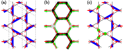
Figure 1: (a) Dimer pattern (blue) and its arrow representation (red); arrows point into the triangle with the dimer. (b) The difference between any allowed arrow pattern (green) and the reference pattern (red) is in one-to-one correspondence to loop patterns. (c) Construction of “dual tension” doping, cf. text.

III Doping the RVB wavefunction

Subjecting the RVB or dimer model to external fields induces doping with elementary excitations: spinons or visons. Spinons are obtained by breaking up a singlet (or dimer) and replacing it by two separate spins (w.l.o.g., two up-spins), which can subsequently separate due to a kinetic term. Visons, on the other hand, correspond to a local disbalance in the relative weight of different singlet (or dimer) configurations (equivalently, loop configurations).

In order to study how a finite density of excitations affects the topological order in the RVB or dimer model, we extend the ansatz to include a tunable quasiparticle doping. Let us start with vison doping: Here, we select a reference dimer pattern $D_{0}$ (=arrow configuration $A_{0}$, Fig. 1a), and adiabatically increase the relative weight of the reference configuration through a filtering $F_{\theta_{v}}=\openone-\theta_{v}\left|\bar{r}\right\rangle\left\langle\bar{r}\right|$ (with $\left|\bar{r}\right\rangle$ the opposite of the reference state) applied to each arrow qubit before the application of $E_{\lambda}$. This directly translates to a “string tension” $(\begin{smallmatrix}1&0\\ 0&1-\theta_{v}\end{smallmatrix})$ in the underlying loop model (defined relative to $D_{0}$) which suppresses longer loops and gives rise to doping with magnetic (vison) excitations; for the dimer point $\lambda=1$, the two doping models are unitarily equivalent.

For spinon doping, we introduce two ansatzes. The first – termed “dual tension” – maps to electric excitations (broken loops). This corresponds to flipped arrows, obtained by applying $G_{\theta_{s}^{\prime}}=\openone+\theta_{s}^{\prime}\sigma_{x}$ Two inpointing arrows are mapped to a singlet, and one (three) to $\left|\uparrow\right\rangle$ ($\left|\uparrow\right\rangle^{\otimes 3}$) (Fig. 1c). However, the resulting ansatz does not correctly reproduce the effect of a local field in lowest order – breaking a singlet into a pair of spinons – as it also yields $4$-spinons-terms. We therefore introduce a second ansatz (“spinon pairs”) by replacing the singlets in $\left|{\bm{\sigma}}(D)\right\rangle$ with a pair of spinons $\left|\uparrow\uparrow\right\rangle$, i.e. changing each singlet to $\tfrac{1}{\sqrt{2}}(\left|\uparrow\downarrow\right\rangle-\left|\downarrow\uparrow\right\rangle)+\theta_{s}^{2}\left|\uparrow\uparrow\right\rangle$. At the dimer point, each spinon is tagged by a third (orthogonal) state $\left|a_{s}\right\rangle$ of the arrow qubit [i.e. $\tfrac{1}{\sqrt{2}}(\left|\uparrow\downarrow\right\rangle-\left|\downarrow\uparrow\right\rangle)\left|a_{\uparrow},a_{\downarrow}\right\rangle+\theta_{s}^{2}\left|\uparrow\uparrow\right\rangle\left|a_{s},a_{s}\right\rangle$], which can be continuously erased through a filtering $\tilde{E}_{\lambda}=3\lambda\openone+(1-\lambda)P$, $P_{ij}=1\,\forall\,i,j$. Unlike the other ansatz, this correctly captures the expected behavior in leading order. We have also found that it performs significantly better as a variational ansatz for the Heisenberg model with magnetic field. We therefore focus on it, and discuss the other ansatz in Appendix B.

IV Results and analysis

We will now study the response of the RVB spin liquid to different fields. For all simulations, we have expressed the wavefunctions as Projected Entangled Pair States (PEPS) [12, 13, 14, 6]; see Appendix A. We use standard numerical PEPS methods (boundary MPS [15, 16, 17]) which allow us to evaluate physical observables in the thermodynamic limit, as well as to extract a correlation length from the boundary MPS. Using the techniques in Refs. 18, 17, we can moreover extract correlation lengths by anyon sector, which label the decay of correlations between a pair of anyons of a certain type. This allows us to microscopically analyze how the system is driven into a trivial phase due to doping with some anyon $a$, causing it to condense – in this process, the mass gap of $a$ decreases until it eventually vanishes and it becomes favorable to have a macroscopic number of $a$ anyons in the ground state: Anyon $a$ has become condensed, leading to a breakdown of topological order [19]. In order to probe the anyon mass $m_{a}$, we can study the anyon-anyon correlation length $\xi_{a}\sim 1/m_{a}$; a diverging $\xi_{a}$ thus indicates condensation of anyon $a$.

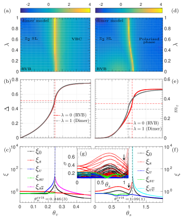
Figure 2: Effect of vison doping (left) and spinon doping (right) (joint $x$ axes). (a,d) Phase diagram, driving the system into (a) a VBC phase and (d) a spin polarized phase, respectively, where the plot shows the logarithm of the correlation length. In both cases, the transition point shows only weak dependence on the RVB-dimer interpolation. (b,e) Response of the wavefunction to doping for RVB and dimer point, again showing very similar behavior. (c,f) Anyon correlations for the RVB as a function of doping, providing an explanation for the robustness (see text). (g) Zoom into (f) including sub-leading correlations, with $y$ axis $\sigma=e^{-1/\xi}$.

We start by considering doping with visons due to lattice anisotropies which drive the system into a vison condensed phase (i.e., a valence bond crystal (VBC)) [21]. Fig. 2a shows the phase diagram as a function of $\lambda$ and the anisotropy $\theta_{v}$. We find that the critical point $\theta_{v}^{\mathrm{crit}}(\lambda)$ is essentially independent of the interpolation $\lambda$ between dimer and RVB. Fig. 2b shows the response to a doping $\theta_{v}$, defined as the difference $\Delta$ between the Heisenberg energies on inequivalent edges, confirming that RVB and dimer model exhibit behave essentially the same way. We can understand this behavior by considering the correlations (mass gaps) for the different anyon types in the RVB state as a function of $\theta_{v}$, Fig. 2c. We find that at the RVB point, the dominant length scale is given by spinon-spinon correlations $\xi_{s}$ [20]. Vison correlations $\xi_{v}$, while present, are only on the order of the topologically trivial correlations $\xi_{t}\approx\xi_{v}$, which in turn are roughly $\xi_{t}\approx\xi_{s}/2$, and thus understood as arising from correlations between two pairs of spinons (which are topologically trivial). That is, the dominant length scale in the system arises from spinons, while visons do not exhibit independent correlations on their own. As we increase the doping $\theta_{v}$, genuine vison correlations start building up, but the overall correlation length remains dominated by the spinon correlations, which do not respond to the vison doping; only very close to the phase transition ($\theta_{v}\approx 0.18$), the vison correlations start to exceed the spinon correlations and diverge at the phase transition.

Next, we consider the effect of magnetic fields, amounting to doping with spinons (the “spinon pairs” ansatz). Fig. 2d shows the phase diagram as a function of the doping $\theta_{s}$ and the dimer-RVB interpolation $\lambda$. Surprisingly, we find that despite the dominant spinon correlations in the RVB state, the phase boundary stays almost constant (the RVB is even slightly more robust). Again, studying the response $m_{z}=\langle\tfrac{1}{N}\sum\sigma_{z}\rangle$ vs. $\theta_{s}$, Fig. 2e, we find two very similar curves, and the RVB shows a smaller response in the relevant regime; as expected, the phase transitions coincide with maximal susceptibility.

These findings are rather counterintuitive, given the dominant spinon correlations in the RVB. To analyze this, we consider the correlations by anyon type, Fig. 2f: We find that the spinon correlation dominates throughout, but it decreases after an initial increase, and exhibits a sharp kink around $\theta_{s}\approx 0.99$ after which it diverges. To study this further, we consider the full spectrum of correlations in Fig. 2g, where we make two noteworthy observations. First, the leading spinon correlation is 4-fold degenerate, where one would have naively expected a spin-$\tfrac{1}{2}$ doublet. Moreover, the correlation in this quadruplet which dominates at small doping is different from the one which finally drives the phase transition – the two lines exhibit a sharp crossing at $\theta_{s}\approx 0.99$, suggesting they are distinguished by some symmetry. Indeed, such a symmetry protection could explain the surprising robustness of the RVB model, since the correlations in the sector driving the phase transition initially decrease under doping.

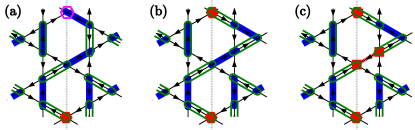
Figure 3: Spinon correlations. Figures show ket-bra overlaps (ket=full symbols, bra=empty symbols). (a,b) Correlations between spinons in (a) ket-bra and (b) ket-ket. Each pattern has a reflection symmetric twin with same (opposite) sign, so that only the ket-bra correlations in (a) survive. (c) Doping with pairs of spinons (red squares) inverts the sign pattern, giving rise to ket-ket correlations. In both cases, only correlations of spins with same $S_{z}$ are possible.

To analyze this further, we first consider the origin of spinon correlations. Correlation functions are overlaps $\langle\psi^{\prime}|\psi\rangle$, where both $\left|\psi\right\rangle$ and $\left\langle\psi^{\prime}\right|$ are RVB states possibly doped with spinons – that is, they are a sum of all singlet coverings, except for one or two static locations where $\left|\uparrow\right\rangle$ spinons are placed. We will call $\left|\psi\right\rangle$ the “ket layer” and $\left\langle\psi^{\prime}\right|$ the “bra layer”. Spinon-spinon correlations are obtained by summing over all overlaps of singlet patterns with the two spinons fixed, Fig. 3, where each pattern yields an amplitude determined by the loop lengths, and the sign follows from the singlet orientations. There are two types of such correlations: A $\uparrow_{\mathrm{ket}}$ spinon (i.e., a single up spin in the ket layer) can be correlated either to a $\uparrow_{\mathrm{bra}}$ spinon, Fig. 3a, or a $\downarrow_{\mathrm{ket}}$ spinon, Fig. 3b (since $S_{z,\mathrm{total}}^{\mathrm{ket}}=S_{z,\mathrm{total}}^{\mathrm{bra}}$); and correspondingly for a $\downarrow_{\mathrm{ket}}$ spinon. We can now explain the 4-fold degeneracy: In the $S_{z}^{\mathrm{total}}=+\tfrac{1}{2}$ sector, either a $\uparrow_{\mathrm{ket}}$ spinon is correlated with $\alpha\uparrow_{\mathrm{bra}}+\beta\downarrow_{\mathrm{ket}}$ in a fixed superposition, or independently $\downarrow_{\mathrm{bra}}$ with a superposition $\alpha\downarrow_{\mathrm{ket}}+\beta\uparrow_{\mathrm{bra}}$. This yields a 2-fold degeneracy, while another factor of $2$ arises from the spin-$\tfrac{1}{2}$ doublet.

However, there is more structure to the spinon-spinon correlations: Every overlap pattern in Fig. 3(a,b) has a “twin” under reflection about the indicated vertical axis. For the singlet orientation chosen, all singlets are flipped under reflection: Thus, overlaps for odd length paths – which connect ket-ket and bra-bra spinons – change their sign under reflection and thus cancel: In the RVB state, only spinons with same $S_{z}$ (equivalently, in opposite layers) can be correlated. Remarkably, this property is preserved under doping (Fig. 3b): Since spinon pairs are symmetric under reflection and do not flip the spin, the paths containing an odd (even) number of spinon pairs which don’t cancel with their reflections are exactly those which correlate spinons with the same $S_{z}$ in the same (opposite) layer. Together with the ket$\leftrightarrow$bra symmetry, this implies that the spinon-spinon correlations can be labelled by sectors $\uparrow_{\pm}:=\uparrow_{\mathrm{ket}}\pm\uparrow_{\mathrm{bra}}$ and $\downarrow_{\pm}:=\downarrow_{\mathrm{ket}}\pm\downarrow_{\mathrm{bra}}$ (that is, sectors which have overlap only with the corresponding superposition of spinons). At the RVB point, they all appear with equal amplitude but opposite phase such that the equal-layer correlations cancel. Crucially, as shown above, this symmetry label is protected by reflection symmetry even at finite doping, preventing mixing. Our analysis is confirmed by numerically computing the matrix elements of $\updownarrow_{\pm}$ with the different correlation sectors. Moreover, analysis of the data shows that the correlations which increase initially are in the $\updownarrow_{-}$ sectors, while those in the $\updownarrow_{+}$ sectors decrease, whereas the phase transition is driven by a diverging correlation length in the $\uparrow_{+}$ sector. However, coupling between the two sectors is prohibited by reflection symmetry. This explains why the system responds to spinon doping with an increased correlation length, and yet, this does not come with a decrease in robustness of the topological phase: the two phenomena take place in different symmetry sectors. A qualitatively similar behavior is observed for the “dual tension” doping: The spinon correlation spectrum again splits in the $\updownarrow_{\pm}$ basis, and we find only a very weak effect on the robustness.

While our analysis is based on a specific doping model, this is in fact a universal behavior, since any perturbation which results in a breaking of singlets into pairs of spinons will have the same effect to leading order. This implies that the initial splitting will again be in the $\updownarrow_{\pm}$ basis, with the $\updownarrow_{-}$ correlations being dominant for small doping, while the $\uparrow_{+}$ correlations drive the phase transition. As long as the perturbation respects the lattice symmetry, these correlation sectors cannot mix, and we therefore expect a qualitatively similar behavior for a general perturbation which induces doping with spinons.

V Conclusions

We have studied the robustness of the RVB and the dimer model on the kagome lattice to perturbations using PEPS. We have found that despite the non-orthogonality of different singlet configurations, the RVB spin liquid exhibits the same robustness to perturbations as the dimer model. For lattice anisotropies (doping with visons), we traced this back to the fact that the length scale induced by the non-orthogonality of singlets gives rise to spinon correlations but does not directly affect the physics of visons. For magnetic fields (doping with spinons), we showed that the robustness arises from a protection of the RVB state due to the reflection symmetry of the lattice, which separates the initially dominating spinon branch from the branch which ultimately drives the phase transition. Our results reveal a surprising universal robustness of the RVB spin liquid against perturbations, highlighting its role as a candidate for the realization of a stable gapped spin liquid.

Appendix A Tensor network implementation of doped RVB

Here, we describe how the different doping mechanisms introduced in the paper can be described as tensor network states, also termed Projected Entangled Pair States (PEPS).

A.1 String tension and dual tension

Let us first describe the PEPS for the RVB with vison and spinon dopings constructed from doping of the underlying loop (or arrow) model, i.e., string tension or dual string tension. This construction will consist of three layers, stacked on top of each other. The lower layer is a PEPS for the loop model with the corresponding (dual) tension. On top of that layer, we apply a PEPO (Projected Entangled Pair Operator) which transforms this loop model into the corresponding dimer model. Finally, in a last step we apply local filtering operations (as introduced in the main text) to the arrow degrees of freedom in the dimer model, which allows to interpolate to the corresponding RVB state.

The PEPS for the first layer – the loop model with tension – consists of two types of tensors: One vertex tensor (without physical legs) and an on-site tensor (which carries the physical index). The vertex tensor has three legs, each of dimension two. We use a computational basis to express the presence or absence of a loop string on the link, and due to the $\mathbb{Z}_{2}$ constraint, the vertex tensor is restricted to four non-zero entries.

$$\begin{split}\vbox{\hbox{\includegraphics[width=25.00003pt]{tc_eps}}}=\ &\delta_{i0}\delta_{jk1}+\delta_{j0}\delta_{ik1}+\delta_{k0}\delta_{ij1}+\delta_{ijk0}.\end{split}$$ (1)

We use $\delta_{i_{1}i_{2}..i_{n}}$ to denote an entry of the $\delta$ tensor with $n$ indices, and the entry is one iff all the indices are equal. The on-site tensor on every link syncs up indices of adjoining vertex tensors and the physical index of the loop model.

$$\vbox{\hbox{\includegraphics[width=27.0pt]{tc_P}}}=\delta_{ija}$$ (2)

After blocking the vertex and the on-site tensors (2), we get the tensor network of the loop model on an infinite lattice (Fig. 4a). We can filter different loop configurations in the diagonal and dual basis by applying a deformation of the form

$$\vbox{\hbox{\includegraphics[width=20.00003pt]{str_ten}}}=\begin{pmatrix}1&\theta_{s}^{\prime}\\ \theta_{s}^{\prime}&1-\theta_{v}\end{pmatrix}$$ (3)

on physical legs. (In the main text, we restrict to the cases where one of the $\theta_{\bullet}\equiv 0$).

The second layer is a PEPO which maps loop configurations on the honeycomb lattice (including broken loops in the case of dual tension) to dimer configurations on the kagome lattice (including monomers in the case of broken loops). It again consists of two types of tensors. The first is a triangular tensor without physical index, which has three indices of dimension three each:

$$\begin{split}\vbox{\hbox{\includegraphics[width=23.99997pt]{eps}}}=\ &\sigma_{ij}\delta_{k2}+\sigma_{jk}\delta_{i2}+\sigma_{ki}\delta_{j2}+\delta_{ijk2}+\\ &\delta_{i0}\delta_{jk2}+\delta_{j0}\delta_{ik2}+\delta_{k0}\delta_{ij2}+\delta_{ijk0}\ ,\end{split}$$ (4)

where the tensor $\sigma=\text{diag}(\frac{1}{\sqrt{2}}\begin{pmatrix}[r]0&-1\\ 1&0\end{pmatrix},0)$ models an oriented singlet and the last four terms correspond to different spinon configurations. The second tensor acts on each site: It takes the loop configuration as an input in index $a$, and outputs a physical spin $p$ and an arrow index $d$, and is built such as to pick the physical qubit from either of the two adjacent virtual indices (and thus triangular tensors (4)), as prescribed by the reference configuration:

$$\begin{split}\vbox{\hbox{\includegraphics[width=30.00005pt]{P}}}=\ \delta_{ad}(&\delta_{d0}\delta_{j2}(\delta_{i0}\delta_{p0}+\delta_{i1}\delta_{p1})+\\ &\delta_{d1}\delta_{i2}(\delta_{j0}\delta_{p0}+\delta_{j1}\delta_{p1}))\ .\end{split}$$ (5)

By design, this tensor is not symmetric in the virtual indices $i$ and $j$, and we use an arrow pointing to the index $j$ to label its orientation. The PEPO (Fig. 4b) is now obtained by assembling (4) and (5) in a hexagonal structure (yielding spins on a kagome lattice), where the arrows need to be oriented such that setting $a\equiv 0$ yields the reference configuration.

The tensor network for the doped dimer model is now obtained by stacking the two tensor networks Fig. 4a (for the honeycomb loop model) and Fig. 4b (for replacing loops with dimers), where the gray indices (labelled $a$) are contracted. The resulting tensor network allows to tune the doping with spinons and visons by changing the parameters $\theta_{s}^{\prime}$ and $\theta_{v}$ in the deformation tensor (3).

Finally, by applying a filtering

$$\vbox{\hbox{\includegraphics[width=20.00003pt]{dimer_ten}}}\equiv E_{\lambda}=\begin{pmatrix}1+\lambda&1-\lambda\\ 1-\lambda&1+\lambda\end{pmatrix}$$ (6)

on the arrow qubits $d$, we can continuously interpolate between the dimer and RVB models also with doping.

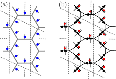
Figure 4: (a) A tensor network of the loop model on the honeycomb lattice with filtering (blue bubble) on each site. (b) PEPO for mapping the loop model to a dimer or RVB model. The on-site tensors are oriented as prescribed by the reference arrow pattern. The incoming (gray) indices are contracted with physical indices in panel (a).

A.2 Doping with spinon pairs

The tensor network to implement the “spinon pair” doping is obtained by modifying the second layer of the preceding construction. There is no longer a need for the first layer (the loop model), since the loop constraint is already contained in the dimer model (see also the original construction for the RVB and dimer PEPS [6]). First, the tensor (4) is modified such that each index has dimension four:

$$\vbox{\hbox{\includegraphics[width=23.99997pt]{eps}}}=\sigma_{ij}\delta_{k2}+\sigma_{jk}\delta_{i2}+\sigma_{ki}\delta_{j2}+\delta_{ijk2}.$$ (7)

Here, the tensor $\sigma=\text{diag}(\frac{1}{\sqrt{2}}\begin{pmatrix}[r]0&-1\\ 1&0\end{pmatrix},0,1)$ encodes either a singlet (in the first two basis states) or the presence of a spinon pair (in the new fourth degree of freedom). Correspondingly, the on-site tensor is also changed to project to the spinon degree of freedom with a tunable weight of $\theta_{s}$, accompanied by a third state $d=2$ of the arrow qubit (the basis state $\left|a_{s}\right\rangle$):

$$\begin{split}\vbox{\hbox{\includegraphics[width=23.99997pt]{pairingP}}}=\ &\delta_{d0}\delta_{j2}(\delta_{i0}\delta_{p0}+\delta_{i1}\delta_{p1})+\\ &\delta_{d1}\delta_{i2}(\delta_{j0}\delta_{p0}+\delta_{j1}\delta_{p1})+\\ &\theta_{s}\delta_{d2}\delta_{p0}(\delta_{i3}\delta_{j2}+\delta_{i2}\delta_{j3})\ ,\end{split}$$ (8)

where the arrows are oriented as before. In order to interpolate to the RVB state, we can erase the information on the dimer indices by applying a deformation

$$\vbox{\hbox{\includegraphics[width=20.00003pt]{dimer_ten}}}\equiv\tilde{E}_{\lambda}=\begin{pmatrix}[r]1+2\lambda&1-\lambda&1-\lambda\\ 1-\lambda&1+2\lambda&1-\lambda\\ 1-\lambda&1-\lambda&1+2\lambda\end{pmatrix}\ .$$ (9)

The final tensor network is identical to Fig. 4b, but without the gray indices.

Appendix B spinon doping with “dual tension”

In this appendix, we report the results for the model with spinon doping constructed through dual string tension.

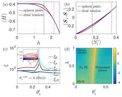
Figure 5: Spinon doping: “dual tension” model. (a) Comparison of variational energies for “spinon pairs” and “dual tension” ansatz as a variational wavefunction for the Heisenberg model with field, Eq. (10); the “spinon pairs” ansatz performs clearly better for most of the parameter regime. Here and in (b), the dashed lines indicate the respective phase transitions. (b) Comparison of Heisenberg energy vs. magnetization for the two models. This illustrates that the two models already differ in the perturbative regime (close to the origin); only the “spinon pairs” ansatz correctly captures the physics of breaking a singlet into a nearest-neighbor pair of spinons in leading order. (c) Correlation functions by spinon sector for the “dual tension” spinon doping; we observe the same characteristic features as in Fig. 2f, which are protected by the same symmetries (in particular lattice reflection) as discussed in the main text. (d) The phase diagram of the dimer-RVB interpolation $\theta_{s}^{\prime}$ for the “dual tension” doping $\lambda$ again exhibits only a weak dependence of the phase transition on changing orthogonal dimers to non-orthogonal singlets.

Fig. 5a provides a comparison of the variational energy for the “dual tension” and the “spinon pairs” ansatz for the Heisenberg Hamiltonian with a transverse field,

$$H=\sum_{\langle ij\rangle}\bm{S}_{i}\cdot\bm{S}_{j}-h\sum_{i}S_{i}^{z}$$ (10)

(with eigenvalues $S_{i}^{z}=\pm\tfrac{1}{2}$). We find that the energy for the “spinon pairs” ansatz is significantly lower, providing a first reason why we chose to consider it as our primary ansatz for spinon doping. Fig. 5b provides further insight into this. It shows the relation between Heisenberg energy $\langle\bm{S}_{i}\cdot\bm{S}_{j}\rangle$ and magnetization $\langle S_{i}^{z}\rangle$: We see that for the same magnetization, the “dual tension” ansatz has a significantly higher Heisenberg energy, which qualitatively means that it requires to break up a correspondingly larger number of singlets to achieve the same magnetization. This effect can be clearly observed in the perturbative regime, i.e., small magnetizations, where the “dual tension” ansatz has a significantly higher slope. We can understand this effect qualitatively in a semi-classical picture: Breaking up a singlet into a pair of spinons leads to a change $\Delta E=1$ in Heisenberg energy, since one singlet is replaced by a $\left|\uparrow\uparrow\right\rangle$ state. On the other hand, the scenario in the “dual tension” construction where flipping an arrow yields $4$ spinons ($3$ on a triangle, and one adjacent vertex) gives rise to a total of four Heisenberg terms having an energy $+\frac{1}{4}$, while before, half of them had energy $0$ and half $-\tfrac{3}{4}$, implying $\Delta E=2.5$ (or $1.25$ per pair of spinons).

Despite these differences, the study of correlations by anyon sectors, Fig. 5c, yields a qualitatively very similar behavior to the case of “spinon pair” doping. In particular, we again observe an additional two-fold degeneracy in the spinon sector (on top of the spin-$\tfrac{1}{2}$ multiplet) which is protected by the lattice symmetry, and which separates the correlations responsible for the phase transitions from those initially responding to the doping; this highlights the fact that this, as we have shown, is a universal effect. Yet again, this symmetry protection is reflected in a rather weak dependence of the phase transition on interpolating between the doped orthogonal dimer model and the doped RVB state, Fig. 5d.

References

- [1] L. Balents, Spin liquids in frustrated magnets, Nature 464, 199 (2010).
- [2] L. Savary and L. Balents, Quantum Spin Liquids, Rep. Prog. Phys. 80, 016502 (2017), arXiv:1601.03742.
- [3] J. Knolle and R. Moessner, A Field Guide to Spin Liquids, Annu. Rev. Condens. Matter Phys. 10, 451 (2019), arXiv:1804.02037.
- [4] P. W. Anderson, Resonating valence bonds: A new kind of insulator?, Mater. Res. Bull. 8, 153 (1973).
- [5] G. Misguich and C. Lhuillier, Two-dimensional quantum antiferromagnets, in Frustrated spin systems, edited by H. T. Diep, World-Scientific, 2003, cond-mat/0310405.
- [6] N. Schuch, D. Poilblanc, J. I. Cirac, and D. Pérez-García, Resonating valence bond states in the PEPS formalism, Phys. Rev. B 86, 115108 (2012), arXiv:1203.4816.
- [7] Z. Zhou, J. Wildeboer, and A. Seidel, Ground state uniqueness of the twelve site RVB spin-liquid parent Hamiltonian on the kagome lattice, Phys. Rev. B 89, 035123 (2014), arXiv:1310.8000.
- [8] D. S. Rokhsar and S. A. Kivelson, Superconductivity and the Quantum Hard-Core Dimer Gas, Phys. Rev. Lett. 61, 2376 (1988).
- [9] G. Misguich, D. Serban, and V. Pasquier, Quantum Dimer Model on the Kagome Lattice: Solvable Dimer-Liquid and Ising Gauge Theory, Phys. Rev. Lett. 89, 137202 (2002), cond-mat/0204428.
- [10] V. Elser and C. Zeng, kagome spin-1/2 antiferromagnets in the hyperbolic plane, Phys. Rev. B 48, 13647 (1993).
- [11] A. Kitaev, Fault-tolerant quantum computation by anyons, Ann. Phys. 303, 2 (2003), quant-ph/9707021.
- [12] F. Verstraete and J. I. Cirac, Renormalization algorithms for Quantum-Many Body Systems in two and higher dimensions, (2004), cond-mat/0407066.
- [13] R. Orus, A Practical Introduction to Tensor Networks: Matrix Product States and Projected Entangled Pair States, Ann. Phys. 349, 117 (2014), arXiv:1306.2164.
- [14] J. C. Bridgeman and C. T. Chubb, Hand-waving and Interpretive Dance: An Introductory Course on Tensor Networks, J. Phys. A: Math. Theor. 50, 223001 (2017), arXiv:1603.03039.
- [15] J. Jordan, R. Orus, G. Vidal, F. Verstraete, and J. I. Cirac, Classical simulation of infinite-size quantum lattice systems in two spatial dimensions, Phys. Rev. Lett. 101, 250602 (2008), cond-mat/0703788.
- [16] J. Haegeman and F. Verstraete, Diagonalizing Transfer Matrices and Matrix Product Operators: A Medley of Exact and Computational Methods, Annual Review of Condensed Matter Physics 8, 355 (2017), arXiv:1611.08519.
- [17] M. Iqbal, K. Duivenvoorden, and N. Schuch, Study of anyon condensation and topological phase transitions from a Z4 topological phase using Projected Entangled Pair States, Phys. Rev. B 97, 195124 (2018), arXiv:1712.04021.
- [18] K. Duivenvoorden, M. Iqbal, J. Haegeman, F. Verstraete, and N. Schuch, Entanglement phases as holographic duals of anyon condensates, Phys. Rev. B 95, 235119 (2017), 1702.08469.
- [19] F. Bais and J. Slingerland, Condensate induced transitions between topologically ordered phases, Phys. Rev. B 79, 045316 (2009), arXiv:0808.0627.
- [20] J. Haegeman, V. Zauner, N. Schuch, and F. Verstraete, Shadows of anyons and the entanglement structure of topological phases, Nature Comm. 6, 8284 (2015), arXiv:1410.5443.
- [21] A. Ralko, M. Ferrero, F. Becca, D. Ivanov, and F. Mila, Crystallization of the resonating valence bond liquid as vortex condensation, Phys. Rev. B 76, 140404(R).