Evidence for reduced magnetic braking in polars from binary population models

Abstract

We present the first population synthesis of synchronous magnetic cataclysmic variables, called polars, taking into account the effect of the white dwarf (WD) magnetic field on angular momentum loss. We implemented the reduced magnetic braking (MB) model proposed by Li, Wu & Wickramasinghe into the Binary Stellar Evolution (bse) code recently calibrated for cataclysmic variable (CV) evolution. We then compared separately our predictions for polars and non-magnetic CVs with a large and homogeneous sample of observed CVs from the Sloan Digital Sky Survey. We found that the predicted orbital period distributions and space densities agree with the observations if period bouncers are excluded. For polars, we also find agreement between predicted and observed mass transfer rates, while the mass transfer rates of non-magnetic CVs with periods ${\gtrsim 3}$ h drastically disagree with those derived from observations. Our results provide strong evidence that the reduced MB model for the evolution of highly magnetized accreting WDs can explain the observed properties of polars. The remaining main issues in our understanding of CV evolution are the origin of the large number of highly magnetic WDs, the large scatter of the observed mass transfer rates for non-magnetic systems with periods ${\gtrsim 3}$ h, and the absence of period bouncers in observed samples.

1 Introduction

Cataclysmic variables (CVs) are interacting binaries composed of a white dwarf (WD) that accretes matter from a low-mass donor star (e.g. Warner, 1995; Hellier, 2001, for comprehensive reviews). Because of their rich variety of variabilities (basically over all wavelengths and on a wide range of time-scales) caused by different physical processes, studying CVs bears relevance for several fields of research including binary formation and evolution, accretion processes, supernova Ia progenitors, and interactions between dense plasma and very strong magnetic fields.

CVs can be classified according to the WD magnetic field strength. Non-magnetic CVs are systems in which the magnetic field is negligible leading to accretion via a disc, which is formed due to angular momentum conservation during mass transfer. Magnetic CVs are systems where the accretion is partially or totally along the WD magnetic field lines. Given that roughly one-third of known CVs in the solar neighborhood are magnetic (Pala et al., 2019a), it is alarming that thorough population synthesis of CVs, in which the WD magnetic field is properly taken into account, has never been carried out.

Magnetic CVs are divided into two main classes, intermediate polars (IPs) and polars (Cropper, 1990; Patterson, 1994; Wickramasinghe & Ferrario, 2000; Ferrario et al., 2015). The main difference between these two types is that in polars, not only the donor spin, but also the WD spin are synchronised with the orbit, presumably because the WD magnetic field exerts a synchronising torque on the donor. In addition, polar WD magnetic fields are of the order of ${10^{7}-10^{8}}$ G, which prevents the formation of an accretion disc. In IPs, the WD spin is not synchronised with the orbit because the WD magnetic field ($\sim 10^{6}-10^{7}$ G) is not strong enough, which implies that most IPs possess truncated accretion discs.

With respect to CV evolution (e.g. Knigge et al., 2011), non-magnetic systems are expected to evolve towards shorter periods due to angular momentum loss (AML) caused mainly by magnetic braking (MB) and gravitational radiation (GR). In the standard CV evolution model, MB dominates the AML above the orbital period gap (orbital periods longer than $\approx 3$ h, e.g. Rappaport et al. 1982), while GR is expected to drive the evolution in CVs with shorter periods (e.g. Paczyński, 1967). The orbital period gap in the standard model is explained via the disrupted MB scenario, which has gained considerable support in the past few years (Schreiber et al., 2010; Zorotovic et al., 2016). MB causes mass transfer rates high enough to drive the main-sequence (MS) donor out of thermal equilibrium, leading to a bloated MS star (about 30 per cent larger in radius). When the donor star becomes fully convective at an orbital period of $\approx 3$ h, MB is expected to cease (or become much less efficient), which leads to a significant drop in the mass transfer rate and a slowdown of the evolution, as the system is now driven by GR only. Such a drop in the mass transfer rate allows the MS donor to re-establish thermal equilibrium (i.e. decrease in size), and eventually the system becomes a detached binary since the secondary is no longer filling its Roche lobe. Even though the system is now detached, it keeps loosing angular momentum due to GR and continues to evolve towards shorter orbital periods. When the orbital period is $\approx 2$ h, the MS donor fills its Roche lobe again, and mass transfer restarts, i.e. the system is again a CV evolving now with relatively low mass transfer rates towards shorter orbital periods. When the period is $\approx 80$ min, the mass loss rate from the secondary drives it increasingly out of thermal equilibrium and it becomes a hydrogen-rich degenerate object. From this point, the donor expands in response to the mass loss, leading to an increase in the orbital period. At this phase, the CV is called a period bouncer. For decades, population models of non-magnetic CVs have been developed, which substantially improved our understanding of non-magnetic CV evolution (e.g. Rappaport et al., 1982; de Kool, 1992; Kolb, 1993; Politano, 1996; Howell et al., 2001; Knigge et al., 2011; Goliasch & Nelson, 2015; Kalomeni et al., 2016; Schreiber et al., 2016; Belloni et al., 2018).

The evolution of polars, however, is most likely different to those of non-magnetic CVs. In these systems the WD magnetic field is expected to affect MB. There are two main evolutionary models that address changes in MB in polars, namely the enhanced MB (e.g. Hameury, King & Lasota, 1989) and the reduced MB (e.g. Li, Wu & Wickramasinghe, 1994; Webbink & Wickramasinghe, 2002) models. Both models assume a coupling of the donor magnetic field lines and the WD magnetic field lines. In the enhanced MB scenario, the wind from the MS donor is trapped by the WD magnetic field lines, which would increase the magnetosphere radius resulting in enhanced AML via MB. This would cause an enhanced mass transfer, leading to correspondingly shorter evolutionary time-scales. In many cases, mass transfer could even be thermally unstable, which would result in a very short life-time for such systems. In contrast, in the reduced MB scenario, winds from the MS donor do not carry away as much angular momentum as in the non-magnetic case resulting in reduced AML via MB. This is because part of the wind remains trapped to the system due to the strong WD magnetic field. Whether the observed population of polars, in particular their orbital period distribution, is consistent with either the enhanced or the reduced MB models, has never been tested.

To progress with this situation, we present here realistic population models of polars. We incorporate the reduced MB scenario in an existing binary population code, and investigate how the WD magnetic field affects CV evolution. We focus on the reduced MB model only because the mass transfer rates in polars derived from observations are smaller than in non-magnetic CVs (Araujo-Betancor & et al., 2005; Townsley & Gänsicke, 2009). These measurements are consistent with reduced AML but clearly contradict enhanced AML. Having incorporated reduced magnetic braking in our CV evolution model, we compare the model predictions with observed orbital periods and mass transfer rates as well as with estimates of the space density.

2 Impact of the WD Magnetic Field on Magnetic Braking

In order to account for the influence of the WD magnetic field $(B_{\rm WD})$ in our simulations, we adopted here the formulation by Webbink & Wickramasinghe (2002, hereafter WW02), which is in turn based on the reduced MB model proposed by Li, Wu & Wickramasinghe (1994, hereafter LWW94).

In a rotating M-dwarf on the main sequence with convective envelope, a dynamo process is able to generate a surface magnetic field (e.g. Schatzman, 1962; Weber & Davis, 1967; Mestel, 1968). If this surface magnetic field is sufficiently strong, it can exert magnetic torques on winds such that co-rotation is established, and the outflowing material follows the magnetic field lines. This way, winds can carry off a substantial amount of angular momentum per unit mass (e.g. Mestel & Spruit, 1987). This is the basic mechanism driving MB. The resulting AML proportionally depends on the stellar rotation (i.e. the greater the star rotation, the greater the wind-driven AML).

More detailed models show, however, that only part of the flow escapes from the star’s surface and that one can separate two regions, a dead zone and a wind zone (e.g. Mestel, 1968, see fig. 1). The dead zone corresponds to the region where gas is prevented from escaping the star due to the pressure of closed magnetic field loops, i.e. the magnetic pressure is greater than the thermal pressure. The wind zone is the region where the field lines are open and gas escapes and carries off angular momentum.

In the case of synchronously rotating CVs (i.e. polars), it is quite likely that $B_{\rm WD}$ affects the interplay between the donor wind and dead zones, as it is strong enough to synchronize both stars of the binary system. LWW94 developed a model for MB in which the donor wind zone is reduced due to the formation of additional closed field lines, which connect the escaping gas directly to the WD. This results in the gas following the WD magnetic field lines, instead of the open M-dwarf magnetic field lines. This causes a reduction of the wind zone, by creating a second dead zone ( LWW94, their fig. 1).

In the model proposed by LWW94, the basic assumptions are: (i) both WD and donor have centred dipole magnetic fields; (ii) the donor magnetic moment is oriented perpendicular to the orbital plane; (iii) the WD magnetic moment $(\mu_{\rm WD})$ is anti-aligned with that of the donor; (iv) the total gas flux carried by open field lines is conserved from the donor to the Alfvén surface. Because of these strong assumptions, the model is clearly simplistic. For instance, $\mu_{\rm WD}$ could have in principle any orientation and Li & Wickramasinghe (1998) showed that detailed evolutionary modelling of polars needs to take into account inclination effects. In addition, the magnetic field may have complex topologies so that adopting dipolar fields might not be adequate. However, it is the only currently available model that can be incorporated in binary population synthesis codes and we test here if it is sufficiently realistic to explain the long-term evolution of polars.

In order to find a description of the limiting lines separating the dead zones and the wind zone, LWW94  assume an isothermal gas and solve the magnetohydrodynamical equations in the dead zones. Based on these solutions, they could estimate the reduction of MB for a given $B_{\rm WD}$. In LWW94, the results are parametrized with the fraction of open field lines $(\Phi)$. In the extreme case of no wind zone, i.e. $B_{\rm WD}$ is strong enough to prevent any MB, $\Phi=0.0$. On the other hand, in the case of negligible $B_{\rm WD}$, the second dead zone does not exist and the MB is not reduced, $\Phi=0.258$. This prescription for the reduction of MB parametrized with $\Phi$ (which depends on the binary parameters and $B_{\rm WD}$) allows to incorporate the impact of strong WD magnetic fields in binary evolution codes.

It has been shown by WW02  that the AML due to MB in polars $(\dot{J}_{\rm MB,pol})$ takes rather a simple form when the donor wind is centrifugally driven:

$$\dot{J}_{\rm MB,pol}\ =\ \dot{J}_{\rm MB,non-mag}\,\left(\frac{\Phi}{0.258}\right)^{5/3}\,,$$ (1)

where $\dot{J}_{\rm MB,non-mag}$ is the AML due to MB in non-magnetic CVs. In this work we used the prescription from Rappaport et al. (1983) with $\gamma=3$, i.e.

$$\dot{J}_{\rm MB,non-mag}\ =\ -5.83\times 10^{-16}\,\left[M_{2}\left(R_{2}\,\Omega_{2}\right)^{3}\right]\ \ {\rm M}_{\odot}\,{\rm R}_{\odot}^{2}\,{\rm yr}^{-2}\,,$$

where $M_{2}$ and $R_{2}$ are the donor mass and radius, respectively, both in solar units, and $\Omega_{2}$ is the donor spin in units of year.

In the standard scenario for CV evolution, the donor MS star becomes significantly bloated as a response to mass transfer in non-magnetic CVs above the orbital period gap. In the model described here, the strongly magnetic WD reduces MB and thus the mass transfer rate in polars. We therefore also expect the secondary to be less bloated in polars. This implies that for polars the critical mass at which MB is disrupted is larger than the critical value of $M_{2}^{\rm crit,non-mag}=0.2$ M_⊙  found for non-magnetic CVs. In the limit of full MB suppression, one would expect that the critical mass is precisely the same as for isolated stars or MS stars in detached binaries, i.e. $M_{2}^{\rm crit,sgl}=0.35$ M_⊙  (e.g. Reiners & Basri, 2009; Schreiber et al., 2010).

If we assume the same dependence on $\Phi$ that has been derived for the angular momentum loss (Eq. 1) for the critical donor mass in polars at which MB is disrupted, $M_{2}^{\rm crit,pol}$, and for the radius increase due to mass loss, we find relatively simple relations for the donor radius and the mass limit of angular momentum loss through MB. The critical mass is then given by

$$M_{2}^{\rm crit,pol}=M_{2}^{\rm crit,sgl}\ -\ \left(M_{2}^{\rm crit,sgl}\ -\ M_{2}^{\rm crit,non-mag}\right)\,\left(\frac{\Phi}{0.258}\right)^{5/3}\,.$$ (2)

and the expansion factor of the MS donor as a function of $\Phi$ in the case MB is reduced is given by

$$f_{\rm bloat,pol}=f_{\rm bloat,non-mag}\,\left(\frac{\Phi}{0.258}\right)^{5/3}\,,$$ (3)

where $f_{\rm bloat,non-mag}\approx 0.357$ (e.g. Davis et al., 2008). This means that in polars the donor radius is approximated as

$$R_{2}^{\rm pol}\ =\ R_{2}^{\rm sgl}\,\left(\,1\ +\ f_{\rm bloat,pol}\,\right)\,,$$ (4)

where $R_{2}^{\rm sgl}$ is the radius of MS single stars or MS stars in detached binaries.

It is important to note that all quantities in Eqs. 1, 2, 3 and 4 are reduced to the standard CV evolution model in case of ${\Phi\geq 0.258}$ (non-magnetic WD). Instead, in the case of extremely high $B_{\rm WD}$, ${\Phi=0.0}$ (highly magnetic WD) our formulation leads to a CV evolution driven only by GR. In this case, the bloating of the donor will negligible and therefore such systems will not evolve through a detached phase, i.e. for them there will be no orbital period gap.

3 The assumed white dwarf magnetic field topology and strengths

For our modelling of reduced MB in polars, we emphasize that in our approach, as in the case of WW02, we assume that the WD is synchronized with the orbit since the onset of mass transfer, i.e. that the system is a polar throughout its evolution with a constant magnetic field strength.

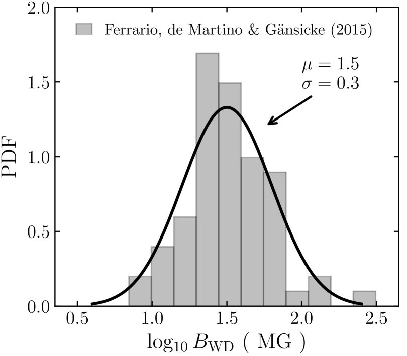
Figure 1: Observed distribution of WD magnetic field in polars, from Ferrario, de Martino & Gänsicke (2015, table 2). The line corresponds to the best-fitting Gaussian $(\mu=1.5;~{}\sigma=0.3)$, which is used to obtain the WD magnetic fields in the simulations.

This approach is justified as we are primarily interested in understanding how an existing $B_{\rm WD}$ affects CV evolution and the predicted period distribution. We therefore used the observed sample of polars which contains 67 polars with measured $B_{\rm WD}$ as listed in Ferrario, de Martino & Gänsicke (2015, table 2). The corresponding $B_{\rm WD}$ distribution is shown in Fig. 1. From this observed $B_{\rm WD}$ distribution, we obtained the best-fitting Gaussian to the $\log_{10}B_{\rm WD}$ distribution, which has mean and standard deviations given by $1.5$ and $0.3$, respectively. As the true distribution might not be a Gaussian, we performed several tests using different probability density functions derived from the observed distributions, such as the kernel density estimation method, and found that the conclusions of this paper are independent of the detailed modelling of the data.

The WD magnetic moment of a given polar in our simulations in given by

$$\mu_{\rm WD}\ =\ \frac{1}{2}\,\left(\,\frac{B_{\rm WD}}{{\rm G}}\right)\,\left(\frac{R_{\rm WD}}{{\rm cm}}\right)^{3}\ \ \ {\rm G\;cm^{3}}\,,$$ (5)

where $R_{\rm WD}$ is the WD radius, and $B_{\rm WD}$ is randomly picked from the probability density function associated with the best-fitting gaussian. As $B_{\rm WD}$ we treat $\mu_{\rm WD}$ in our simulations as being constant, for a particular polar throughout its evolution.

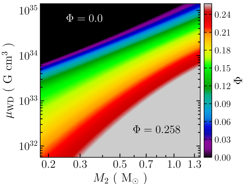
Figure 2: The fraction of open field lines $(\Phi)$ as a function of the donor mass $(M_{2})$ and the WD magnetic moment $(\mu_{\rm WD})$. The black area defines the region where the magnetosphere is completely closed ${({\Phi=0.0})}$, which provides that MB is completely suppressed, and only GR plays a role in the polar evolution. The gray area corresponds to the non-magnetic case ${({\Phi=0.258})}$.

In order to infer the value of $\Phi$, we utilized fig. 3 in WW02, who showed that $\Phi$ is mainly a function of $\mu_{\rm WD}$ and $M_{2}$, depending only very weakly on $M_{\rm WD}$. In that figure, five values of $\Phi$ are given, from 0.0 to 0.2, in steps of 0.05. We then linearly interpolate/extrapolate these curves to find the value of $\Phi$ for each polar in our simulations. The procedure is illustrated in Fig. 2, which shows the distribution of $\Phi$ in the plane $\mu_{\rm WD}$ versus $M_{2}$. If a given polar in that plane belongs to the region where $\Phi=0.00$ (black area in the figure), MB is assumed to be absent, and the evolution is driven by GR only. Otherwise, MB is still present, and has its strength reduced as $\mu_{\rm WD}$ becomes larger or $M_{2}$ becomes smaller. In the region where $\Phi=0.258$ (gray area in the figure), the evolution of the systems is assumed to be that of a non-magnetic CV. Unlike $B_{\rm WD}$ and $\mu_{\rm WD}$, $\Phi$ is not constant for a given polar. Indeed, as shown in Fig. 2, $\Phi$ depends on both $\mu_{\rm WD}$ and $M_{2}$. Since $M_{2}$ decreases with time, as a result of mass transfer during CV evolution, polars evolve through Fig. 2 from right to left at constant $\mu_{\rm WD}$. Hence, for each time-step, $\Phi$ and the properties that depend on it (Eqs. 1, 2, 3 and 4 ) need to be updated. A comparison between our approach and WW02 is provided in Appendix A.

4 Binary Population Modelling

To carry out our simulations, we utilized the Binary Star Evolution (bse) code (Hurley et al., 2000, 2002), updated  by Belloni et al. (2018). bse models AML mechanisms, such as GR and MB, and mass transfer occurs if either star fills its Roche lobe and may proceed on a nuclear, thermal, or dynamical time-scale. The current version of the bse code includes state-of-the-art prescriptions for CV evolution, which allows accurate modelling of these interacting binaries. More details can be found in Belloni et al. (2018).

Our modelling here follows a similar approach to that in Belloni et al. (2018). We carried out binary population synthesis using an initial population of $2\times 10^{8}$ objects (single and binary stars) assuming solar metallicity (i.e. $Z=0.02$). The properties of the binary stars are assumed to follow particular distributions. First, the primary is picked from the Kroupa (2001) initial mass function enforcing that ${1~{}{\rm M}_{\odot}~{}\leq~{}M_{1}~{}\leq~{}8~{}{\rm M}_{\odot}}$. The secondary is then drawn from a uniform mass ratio distribution, ensuring that $M_{2}\leq M_{1}$, and that ${M_{2}\geq 0.07}$ M_⊙. The semimajor axis ${(10^{0.5}~{}{\rm R}_{\odot}~{}\leq~{}a~{}\leq~{}10^{4.5}~{}{\rm R}_{\odot})}$ and the eccentricity ${(0~{}\leq~{}e~{}\leq~{}1)}$ are assumed to follow a log-uniform and a thermal distribution, respectively. Single stars are generated from the same initial mass function as the primaries in binaries.

Regarding common-envelope evolution, we adopted a low efficiency, i.e. we assumed that 25 per cent of the dissipated binary orbital energy is used to expel the common envelope. The binding energy parameter was calculated according to Claeys et al. (2014) assuming that contributions from recombination energy are negligible (e.g. Zorotovic et al., 2010; Toonen & Nelemans, 2013; Camacho et al., 2014; Cojocaru et al., 2017; Belloni et al., 2019).

As the bse code cannot handle thermal time-scale mass transfer, we do not consider CVs emerging from this channel. This appears to be a reasonable assumption as observations show that only $\approx 5$ per cent of all CVs originate from this phase (Pala et al., 2019a).

Finally, the consequential angular momentum prescription adopted here is the one postulated by Schreiber et al. (2016), which is currently the only model that can explain crucial observations related to CV evolution, such as the space density, the orbital period and WD mass distributions (Schreiber et al., 2016; Belloni et al., 2018; McAllister et al., 2019). Furthermore, it also provides an explanation for the properties of detached CVs crossing the orbital period gap (Zorotovic et al., 2016), the existence of single He-core WDs (Zorotovic & Schreiber, 2017), and the mass density of CVs in globular clusters (Belloni et al., 2019).

As in Goliasch & Nelson (2015) and Belloni et al. (2018), we assumed that the initial mass function is constant in time and that the binary fraction is 50 per cent (consistent with the binary fraction of WD primary progenitors, see Patience et al., 2002). Additionally, during the Galactic disc life-time, which is here assumed to be $\approx$ 10 Gyr (Kilic et al., 2017), we adopted a constant star formation rate (e.g. Weidner et al., 2004; Kroupa et al., 2013; Recchi & Kroupa, 2015; Schulz et al., 2015). This implies that the birth-time distributions of both binary and single stars are uniform. The generated populations of single and binary stars are then evolved with the bse code from the birth time until the assumed Galactic age of 10 Gyr.

The CV space density is calculated following the scheme presented in Goliasch & Nelson (2015, see their sections 2.2.3 and 2.2.4). As we generate both single stars and binaries, we can normalize the results of our population synthesis such that the number of single WDs corresponds to a specific birth rate of WDs in the Galactic disc. We adopt a WD space density of $\sim 5\times 10^{-3}$ pc^-3 (Holberg et al., 2008, 2016; Jiménez-Esteban et al., 2018; Hollands et al., 2018) and a WD birth rate of $\sim 10^{-12}$ pc^-3 yr^-1 (Vennes et al., 1997; Holberg et al., 2016), which implies a WD formation rate of $\sim 0.4$ yr^-1, and provides a total number of $\sim 4\times 10^{9}$ WDs in the disc. In order to derive the absolute number of systems that should be present in the Galactic disc, we similarly scaled the total number of CVs. The space density is then computed by assuming a Galactic volume of $5\times 10^{11}$ pc³ (e.g. Toonen et al., 2017).

Finally, in our simulations, we assume that the fraction of polars relative to the entire CV population is $\simeq 28$ per cent, which is the measured fraction of polars in the solar neighbourhood (Pala et al., 2019a). To simulate polar and non-magnetic CV evolution simultaneously we defined at the onset of mass transfer whether the CV is non-magnetic or polar assuming a probability of 28 per cent of being a polar. The field strengths for the selected polars were than randomly drawn from the observed field strength distribution described in Section 3.

5 Comparing model predictions and observations

In order to compare our predicted orbital period distributions with observations, we searched for all CVs with accurate orbital period determinations from the Sloan Digital Sky Survey (SDSS). We found 199 systems, which are listed in Table 2. SDSS provides both photometric and spectroscopic data, and allows the unambiguous identification of CVs from hydrogen and helium emission lines. In addition, its deep magnitude limit allows the detection of intrinsically faint systems (Gänsicke et al., 2009), characterized by low accretion rates, even at several scale heights above the Galactic plane. This makes this sample one of the largest homogeneous CV samples available, as its broad colour selection range is superior to any previous surveys.

Recently, Pala et al. (2019a) investigated the intrinsic Galactic CV population in a volume-limited sample of CVs, which is about 75 per cent complete. This sample was built using accurate parallaxes provided by the Gaia Data Release 2 parallax measurements and is composed of 42 CVs within 150 pc, including two newly discovered systems. The derived CV space density is clearly better than all previous estimates with high accuracy and small errors. In addition, they measured the intrinsic fraction of CVs above and below the orbital period gap as well as the fraction of magnetic CVs. As the 150 pc sample is very small, we compare the predicted orbital period distributions with the homogeneous and large SDSS sample. We consider the less biased, but small, 150 pc sample for the comparison between predicted and observed space densities and fractions of period bouncers.

To confront predicted mass transfer rates with observations, we compare predicted and observed effective temperatures of the WDs in CVs. The effective temperatures of these WDs are known to be reasonable tracers of the mean mass transfer rates, as they depend on compressional heating caused by the accreted matter (e.g. Townsley & Bildsten, 2003, 2004). When the mass transfer rate is rather low, for dwarf novae in quiescence, or polars and nova-likes in the low state, the emission is dominated by the WD surface, and the measurement of the WD effective temperature is possible. For the comparison of observed and predicted effective temperatures we used the samples from Pala et al. (2017, and references therein, for non-magnetic CVs) and Townsley & Gänsicke (2009, and references therein, for polars). These authors provide lists of CVs with reliable WD effective temperature measurements and they contain in total 59 non-magnetic CVs and 13 polars. We excluded from the observational sample the six non-magnetic systems with evolved donors reported by Pala et al. (2017), namely V485 Cen, QZ Ser, SDSS J013701.06$-$091234.8, SDSS J001153.08$-$064739.2, BD Pav, and HS 0218$+$3229, since we do not account for this evolutionary channel in our simulations.

6 Results

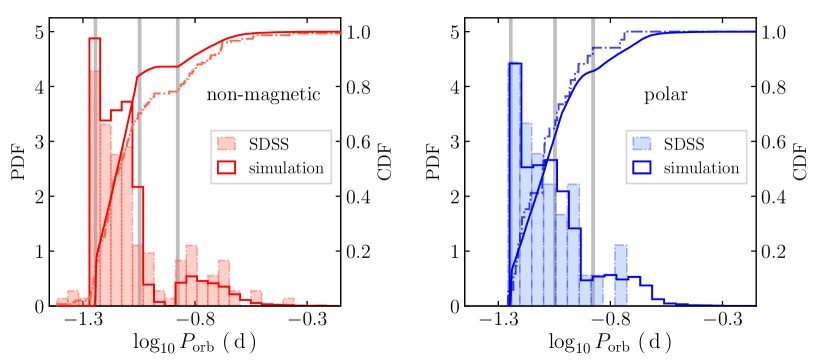
Figure 3: Comparison between observed and predicted orbital period $(P_{\rm orb})$ distributions for both non-magnetic CVs (left-hand panel) and polars (right-hand panel). Observed measurements for non-magnetic CVs and polars are from SDSS data (Table 2). Vertical lines in the period distribution are the observational location of the period minimum (Gänsicke et al., 2009) and gap edges (Knigge, 2006). Notice that distributions for both non-magnetic CVs and polars strongly differ from each other. See text for more details.

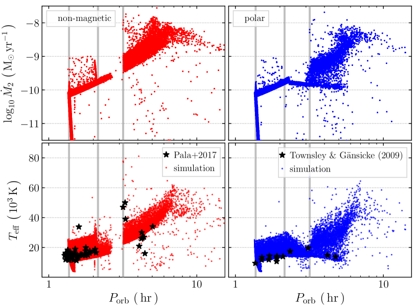
Figure 4: Predicted mass transfer rate ($\dot{M}_{2}$, top panels) and WD effective temperature ($T_{\rm eff}$, bottom panels) against the orbital period ($P_{\rm orb}$). In the left-hand panels non-magnetic CVs are shown, and in the right-hand panels polars are depicted. Observed values related to $T_{\rm eff}$ are shown as black stars and are from Pala et al. (2017, and references therein, for non-magnetic CVs) and Townsley & Gänsicke (2009, and references therein, for polars). Vertical lines in the period distribution are the observational location of the period minimum (Gänsicke et al., 2009) and gap edges (Knigge, 2006). Notice that mass transfer rates of polars above the orbital period gap are in general smaller than those of non-magnetic CVs, which consecutively results in smaller $T_{\rm eff}$ amongst polars.

We concentrate the analysis of our population synthesis outcomes on three very important CV observables, namely the orbital period distribution, the mass transfer rate distribution (or alternatively the WD effective temperature distribution) and the space density. While comparing the orbital period distributions, we will consider only systems with donor masses greater than $0.05$ M_⊙, i.e. we neglect period bouncers. The reason is twofold. First, the mass-radius relation for CV donors having $M_{2}<0.05$ M_⊙ is not reliable (Knigge et al., 2011). Secondly, period bouncers are extremely rare in observed samples (e.g. Hernández Santisteban et al., 2018; Pala et al., 2019a). The observed sample of period bouncers is therefore most likely much more biased and incomplete than the sample of brighter CVs.

6.1 Orbital period distribution

Starting with the observed distributions (NON-MAG and POLAR systems in Table 2), we see a gap in the orbital period distribution of non-magnetic CVs, while the same feature is absent in polars. Indeed, the fraction of non-magnetic CVs inside the gap (i.e. 2 h $<$ $P_{\rm orb}$ $<$ 3 h) is $\approx 8$ per cent, while for polars this fraction is much larger, being $\approx 25$ per cent. We also see a larger fraction of non-magnetic CVs above the gap in comparison to polars. In particular, the fraction of polars with periods longer than $\approx 3$ h is only $\approx 9$ per cent, while $\approx 21$ per cent of non-magnetic CVs are located above the gap. These two features put together suggest that both observed distributions are intrinsically different, even though we still rely on relatively small-number statistics for such a claim.

In agreement with observations, our population synthesis shows significant differences in the predicted orbital period distributions. On the left-hand panel of Fig. 3, we compare the predicted orbital period distribution of non-magnetic CVs with the observed one. Notice that the results from our simulation reasonably well reproduce the main features of the observed distribution, i.e. the orbital period gap between $\approx 2$ and $\approx 3$ h, and the accumulation of systems close to the orbital period minimum ($\approx 80$ min). We can also reasonably well reproduce the decreasing number of systems above the orbital period gap towards longer periods. The orbital period distribution of polars (right-hand panel of Fig. 3) differs from the distribution of non-magnetic CVs. In the polar case, instead of presenting an orbital period gap, polars gradually fill the region between $\approx 2$ and $\approx 3$ h, as a consequence of the reduction of AML through MB. Indeed, for sufficiently high values of $\mu_{\rm WD}$, MB becomes considerably less efficient, which leads to smaller mass transfer rates above the orbital period gap and donors less bloated. As a consequence, the contraction of the donor stars in these systems when MB is disrupted is less significant and the polar needs less time to become semidetached again. The overall effect is a dilution of the gap, as a relatively large number of polars penetrates the region of the gap when mass transfer turns on again. Concerning the orbital period minimum, we do not detect significant difference between polars and non-magnetic CVs. In both cases we detect a peak at $\approx 80$ min.

In order to evaluate whether our results are consistent with observed distributions on statistical grounds, we applied two-sample Kolmogorov–Smirnov tests. The null hypothesis of each test is that both predicted and observed distributions stem from the same parent population. Comparing predicted and observed distributions in the non-magnetic case, the $p$-value is 0.001, which indicates that our predicted distribution differs from the observed one, even though we can clearly reproduce key features of the observed distribution. The reason for that is likely an observational bias against the detection of short-period systems. Regarding polars, the $p$-value is ${\approx 0.53}$. This provides strong support to the null hypothesis that both distributions stem from the same parent distribution. Consequently, this suggests that the reduced MB prescription represents an appropriate model to explain polar evolution.

6.2 Mass transfer rates and WD effective temperatures

A direct consequence of the reduced MB model in polars is the reduction of their mass transfer rates above the orbital period gap, as well as the slow-down of the evolution. In the top row of Fig. 4 we compare predicted mass transfer rates $(\dot{M}_{2})$ against the orbital period of non-magnetic CVs (left-hand panel) and polars (right-hand panel). Note that, as expected, both classes have similar mass transfer rates below the orbital period gap $(\sim 10^{-10}$ M_⊙ yr${}^{-1})$. However, above the gap, most non-magnetic CVs have mass transfer rates between $10^{-9}$ and $10^{-8}$ M_⊙ yr^-1, while most polars have ${\dot{M}_{2}\lesssim 10^{-9}}$ M_⊙ yr^-1. This is a difference of one to two orders of magnitude.

A way of testing whether such predictions are consistent with observations is by means of the WD effective temperature. The WD effective temperatures in CVs trace the mean mass transfer rate as the WD is heated by the energy released by fluid elements as they are compressed by further accretion (Townsley & Bildsten, 2003, 2004). The WD effective temperature ($T_{\rm eff}$) due to this compressional heating is given by (Townsley & Gänsicke, 2009, eq. 2)

$$\frac{T_{\rm eff}}{{\rm K}}\ =\ 1.7\times 10^{4}\;\left(\,\frac{\langle\,\dot{M}_{2}\,\rangle}{10^{-10}\,{\rm M}_{\odot}\,{\rm yr}^{-1}}\,\right)^{0.25}\;\left(\,\frac{M_{\rm WD}}{0.9\,{\rm M}_{\odot}}\,\right),$$ (6)

where $\langle\dot{M}_{2}\rangle$ and $M_{\rm WD}$ are the average mass transfer rate and the WD mass, respectively. However, this approach is only correct if the WD cooling temperature is smaller than the temperature derived from compressional heating. We therefore also determined the WD cooling temperature as in Zorotovic & Schreiber (2017), i.e. via interpolation of DA (pure hydrogen atmosphere) WD evolutionary models by Althaus & Benvenuto (1997), for helium-core WDs, and by Fontaine et al. (2001), for carbon/oxygen-core WDs. Having calculated both the cooling and the compressional heating temperatures, we took the higher temperature for each WD produced by our population model.

In the bottom row of Fig. 4, we compare predicted and observed $T_{\rm eff}$ of non-magnetic CVs (left-hand panel) and polars (right-hand panel). Observed values are from Pala et al. (2017, and references therein) and Townsley & Gänsicke (2009, and references therein). As in the case of the mass transfer rate, below the gap both CV types have similar $T_{\rm eff}$ in the range of ${\sim 10\,000-20\,000}$ K, and are in general in agreement with the observations. However, the predicted $T_{\rm eff}$ above the gap drastically differ from each other. As the mass transfer rates are smaller for polars in this period range, so are the values of $T_{\rm eff}$ (Eq. 6). While the temperatures for non-magnetic CVs are usually greater than $\sim 30\,000$ K, those of polars are in general smaller than that.

The predicted and observed $T_{\rm eff}$ of polars seem to agree with each other, even though this claim is weaker for systems above the orbital period gap, due to small-number statistics. Regarding non-magnetic CVs, our predicted $T_{\rm eff}$ provides reasonable results below the orbital period gap as most systems fall in the predicted range with the exception of one system. This CV (SDSS J153817.35$+$512338.0) could be either a young CV or recently had a nova explosion (Pala et al., 2017). However, above the gap, only two systems (out of 10) are consistent with predicted values. The remaining systems are either above (nova-likes) or below (dwarf novae) the range of predicted $T_{\rm eff}$ which represents a striking disagreement between observations and theory. In any event, our results concerning polars are encouraging and, together with the already-mentioned orbital period distribution, provide strong support for the reduced MB model.

6.3 Space density

The last aspect we will address is the space density. The numbers of polars and non-magnetic CVs produced in our simulations are provided in Table 1, together with the space density, computed as described in Section 4. By construction, the predicted fraction of polars ($\approx 25$ per cent) matches that found in observations, which is $\approx 28$ per cent (Pala et al., 2019a). The predicted space densities for all CVs, non-magnetic CVs and polars are ${\approx 2.2^{+2.2}_{-1.1}\times 10^{-5}}$, ${\approx 1.6^{+1.6}_{-0.8}\times 10^{-5}}$ and ${\approx 5.2^{+5.2}_{-2.6}\times 10^{-6}}$ pc^-3, respectively. When removing the period bouncers, those space densities are ${\approx 4.5^{+4.5}_{-2.3}\times 10^{-6}}$, ${\approx 3.0^{+3.0}_{-1.5}\times 10^{-6}}$, and ${\approx 1.5^{+1.5}_{-0.8}\times 10^{-6}}$ pc^-3, respectively. Due to uncertainties in the initial binary populations these space densities might be affected by a factor of $2$.

Table 1: Number and space density of non-magnetic CVs and polars in our simulations. The column labelled Model presents results from our simulations, while the column labelled Absolute shows the numbers scaled according to the birth rate of single WDs. Finally, the space density ($\rho$) was calculated with the absolute numbers, assuming a Galactic volume of $5\times 10^{11}$ pc³. The errors are estimated from uncertainties in the initial binary population. In the last four columns we provide the fractions of long-period, short-period and gap CVs, and period bouncers. Finally, in the last column, we provide the space density when period bouncers are excluded.

CV type Model Absolute $\rho$ $f_{\rm long}$ $f_{\rm short}$ $f_{\rm gap}$ $f_{\rm bouncers}$ $\rho$ (without bouncers) $\left(~{}10^{6}~{}\right)$ $\left(~{}10^{-6}~{}{\rm pc}^{-3}~{}\right)$ (per cent) (per cent) (per cent) (per cent) $\left(~{}10^{-6}~{}{\rm pc}^{-3}~{}\right)$ all CVs $324509$ $10.732$ ${21.5^{+21.5}_{-11.3}}$ $2.9$ $11.2$ $4.1$ $81.8$ ${4.5^{+4.5}_{-2.3}}$ non-magnetic $245393$ $8.116$ ${16.2^{+16.2}_{-8.1}}$ $2.4$ $11.2$ $2.4$ $84.0$ ${3.0^{+3.0}_{-1.5}}$ polar $79116$ $2.616$ ${5.2^{+5.2}_{-2.6}}$ $4.3$ $11.3$ $9.3$ $75.1$ ${1.5^{+1.5}_{-0.8}}$

Predicted space densities are in reasonable agreement with observations, within the errors. For example, using 20 non-magnetic CVs, Pretorius & Knigge (2012) determined a space density of ${4^{+6}_{-2}\times 10^{-6}}$ pc^-3, from the ROSAT Bright Survey and the ROSAT North Ecliptic Pole survey, which are supposedly complete X-ray flux-limited surveys. Schreiber & Gänsicke (2003) derived a lower limit of ${\sim 10^{-5}}$ pc^-3 for the space density of post-common-envelope binaries that are CV progenitors. Hernández Santisteban et al. (2018) estimated an upper limit for the period bouncer space density of ${\lesssim 2\times 10^{-5}}$ pc^-3 using SDSS Stripe 82 data. Schwope (2018), who took into account recent distance measurements from the Gaia satellite in previous determinations using ROSAT surveys, measured a space density of non-magnetic CVs to be ${\sim 10^{-6}-10^{-5}}$ pc^-3, depending on the assumed scale height and survey. Regarding polars, Pretorius et al. (2013) used 24 systems from the X-ray flux-limited ROSAT Bright Survey sample and estimated a space density of ${9.8^{+5.4}_{-3.1}\times 10^{-7}}$ pc^-3, provided that their high-state duty cycle are 0.5 and that they are below the survey detection limit during their low states.

Most recently, Pala et al. (2019a) determined space densities with unprecedented small uncertainties. Their measured values are ${4.8^{+0.6}_{-0.9}\times 10^{-6}}$ and ${1.2^{+0.4}_{-0.5}\times 10^{-6}}$ pc^-3, for all and magnetic CVs, respectively, assuming a scale height of 280 pc. These space densities are the most reliable ones derived from observations so far and are smaller by a factor of $2-6$ than our predictions. However, if we exclude period bouncers from both predicted and observed samples (2 out of 42 systems in the 150 pc sample are potentially period bouncers), the predicted and observed space densities are in very good agreement.

We also show in Table 1 the relative fractions of simulated systems in different period ranges. It is clear from the table that the fraction of polars inside the gap is much larger than that of non-magnetic CVs (about four times). In addition, the fraction of polars above the gap is also larger (about two times). Moreover, there is a reduction of about 10 per cent of period bouncers in polars, and both have similar fractions of systems between the period minimum and the lower edge of the gap. The different fractions for non-magnetic and polar CVs, are caused by different characteristic evolutionary time-scales. Indeed, in the reduced MB model, polars are less affected by MB (several only by GR), due to the strong influence of their high WD magnetic field on MB. On the other hand, non-magnetic CV evolution above the gap is driven by AML due to full MB, which is around one order of magnitude stronger than GR, and greater than any reduced MB. This results in a faster evolution for non-magnetic systems, in comparison with polars. Therefore, the relative number of polars above the gap is larger than for non-magnetic CVs. For the same reason, less polars manage to become period bouncers.

Excluding period bouncers (which either seem to be difficult to find or are over predicted by our model), the predicted fraction of all CVs above the gap is $\approx 16$ per cent. This prediction is in excellent agreement with the observations. Pala et al. (2019a) found that ${\approx 17.5}$ per cent of all CVs are above the orbital period gap, when their $\approx 5$ per cent period bouncer candidates are removed from the analysis.

7 Discussion

We have shown in Section 6 that the space densities and orbital period distribution of both non-magnetic CVs and polars agree well with observations if period bouncers are excluded from the analysis. In addition, the mass transfer rates of polars also seem to agree with the observations while those predicted for non-magnetic CVs cannot reproduce the mass transfer rates derived from observations for systems above the gap. Here, we will discuss potential caveats in both simulations and observations.

7.1 Is the SDSS CV sample biased against short-period systems?

We showed in Section 6.1 that the reduced MB model proposed by LWW94 is capable of providing a satisfactory explanation for differences in the observed orbital period distributions of non-magnetic CVs and polars. Even though our predicted orbital period distribution for non-magnetic CVs exhibits the key features of the observed distribution, we found statistical evidence supporting the hypothesis that they do not stem from the same parent population. Such a result is likely due to observational biases involved in the SDSS CV sample.

As discussed in Gänsicke et al. (2009), SDSS covers high Galactic latitudes ($|b|>30^{\rm o}$) and could identify long-period CVs out to a distance of $\gtrsim 10^{4}$ pc, while WD-dominated CVs are found only out to a distance of $\sim 300$ pc. This difference in distance illustrates the bias towards long-period CVs in comparison to CVs with shorter periods. Further evidence is provided in Fig. 5, which shows the cumulative distributions of SDSS CV distances for CVs whose distance measurements have errors smaller than $30$ per cent. Approximately $3/4$ of the CVs in the SDSS sample fulfil this criterion. The average distance for non-magnetic CVs with periods longer than 3 h is $1\,206\pm 666$ pc, while for non-magnetic CVs with periods shorter than 2 h, it is $422\pm 231$ pc. Consequently, a better agreement between predicted and observed distributions would likely be achieved if more short-period non-magnetic CVs could be detected, whose reduced relative number is expected to be a consequence of the limiting magnitude of the SDSS.

Provided that both non-magnetic CV and polar samples come from SDSS, one might ask why the bias previously discussed does not influence the comparisons in the case of polars, in which we found that both predicted and observed distributions are consistent and likely stem from the same parent population. Figure 5 shows the cumulative distribution of polar distances, for those with reliable distance measurements (error smaller than 30 per cent). On average, polars have distances of $369\pm 183$ pc, which implies that they are considerably closer than long-period non-magnetic CVs. Due to reduced MB the mass transfer differences in polars and its dependence on orbital period are much smaller than in non-magnetic CVs. Therefore the distance/magnitude bias is weaker than in non-magnetic CVs and the SDSS polar sample is more representative of the true polar population in the Galaxy. In order to verify this we performed a two-sample Kolmogorov–Smirnov test taking into account both the SDSS polar sample (34 systems) and the 150 pc polar sample (12 systems). The $p$-value is $\approx 0.151$, which does not allow us to reject the null hypothesis that indeed both distributions stem from the same parent population.

Regarding the relative incidence of non-magnetic CVs above and below the orbital period gap, we note that we predict similar fractions of systems below the orbital period gap than found in the SDSS CV sample. The fraction of non-magnetic CVs above the orbital period gap in the SDSS sample is $21\pm 3$ per cent, and $79\pm 3$ per cent are either in the orbital period gap or below. The same fractions in the predicted population (excluding period bouncers) are $15$ and $85$ per cent, respectively. In the 150 pc sample (Pala et al., 2019a), the same fractions for non-magnetic CVs are $18\pm 7$ and $82\pm 7$ per cent, which are very close to the predicted values.

We therefore conclude that the SDSS sample is clearly still biased towards long-period non-magnetic systems and that this is likely the reason for the disagreement in the left-hand panel of Fig. 3.

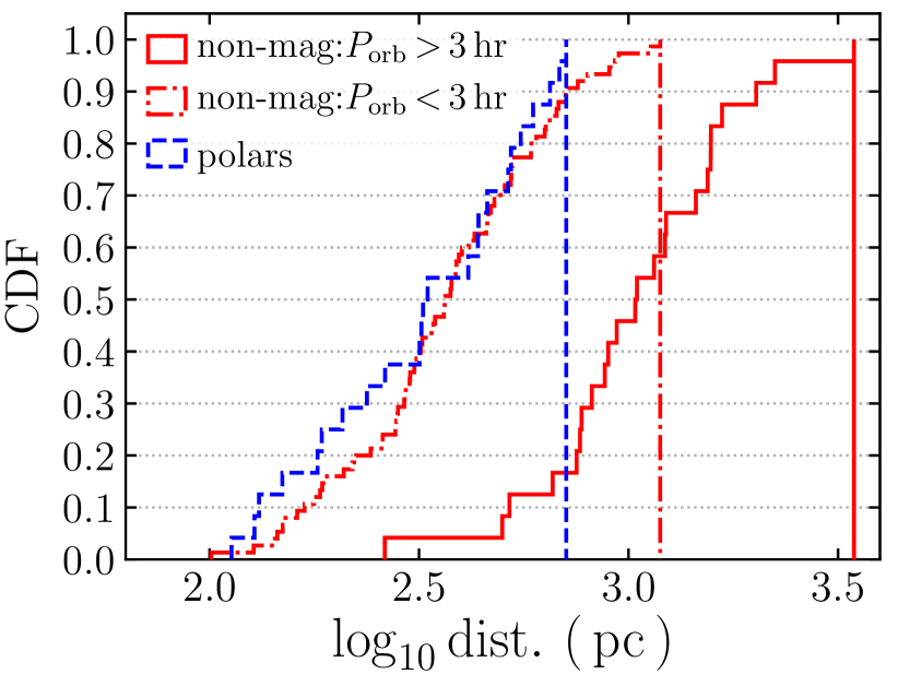
Figure 5: Cumulative distribution of SDSS CV distances whose measurements are reliable (errors smaller than 30 per cent). The red solid line is for non-magnetic CVs with periods longer than 3 h, the red dot-dashed line is for non-magnetic CVs with periods shorter than 3 h and the blue dashed line is for polars. Notice that the distances to polars are on average smaller, followed by short-period non-magnetic CVs. Non-magnetic CVs above the orbital period gap have on average the largest distances among SDSS CVs.

7.2 What problems are still standing in CV evolution?

In Section 6.3, we computed the space densities for non-magnetic CVs and polars and they are generally in good agreement with previous and rather crude observational estimates. The by far most reliable measurements of CV space densities (Pala et al., 2019a), however, are a factor of $2$–$6$ smaller than our predictions. This is entirely caused by the fact that our models predict $80$ per cent of all CVs to be period bouncers while only $\simeq 5$ per cent of the CVs within 150 pc seem to be period bouncers. If we compare the space densities of CVs prior to the period minimum, our predictions perfectly agree with the space densities derived from the 150 pc sample.

We see two possible explanations for this disagreement between predicted and observed number of period bouncers. First, the absence of period bouncers in the 150 pc sample could mean that they do not exist in numbers as large as predicted by our evolutionary models. This suggests that CVs reach the period minimum (because the period distribution below the gap roughly agrees with the predictions) but that they have not had time to evolve past the period minimum. This would imply that the time-scale for an initial binary to evolve into a CV would be significantly longer and the currently observed CVs would therefore be significantly older systems (the initial binary was born earlier). Alternatively, even the 150 pc sample could miss a large number of existing period bouncers as their mass transfer rates can be extremely low and their outburst frequency can be extremely long. Dedicated deep surveys for period bouncers are the only possibility to solve this issue.

Regarding mass transfer rates and WD effective temperatures due to compressional heating, we showed in Section 6.2 that our results are in good agreement with observed values of polars and non-magnetic CVs below the orbital period gap. However, as we can clearly see from Fig. 4, predicted values for non-magnetic CVs above the gap drastically disagree with observations. This issue is very likely not caused by an observational bias, as some of the systems the model does not reproduce have higher and others have lower temperatures than predicted by our model.

In general we see two possibilities to solve this puzzle. First, the measured WD effective temperatures could not represent a good proxy of the accretion rate. Indeed, the temperature of the WD is only sensitive to variations of the mass transfer rate on time-scales that are much shorter than those produced by the most likely types of long-term fluctuations (e.g. irradiation-driven cycles or nova-induced variations, Knigge et al., 2011), which could result in unreliable estimates of the secular/average mass transfer rate for some systems. More importantly, in CVs that have undergone many nova eruptions, the WD cooling could be affected by changes in the structure of its outer envelope and for these systems the accretion rate could thus be overestimated by only considering compressional heating.

At first glance, this idea appears plausible because most novae are observed in the period range above the gap, especially between $3$ and $4$ h, exactly where the high-temperature WDs are found (Tappert et al., 2017). However, if the mass transfer rates were much lower than those derived from compressional heating, the cooling time-scale of WDs heated by nova eruptions (Prialnik, 1986) would be about an order of magnitude shorter than the corresponding nova cycle. To have caught all three systems in the $3$–$4$ h period range in the relatively short post-nova phase therefore appears to be extremely unlikely. It seems more plausible to assume that the origin of the high temperatures are large mass transfer rates. As shown by Townsley & Bildsten (2005), the accumulation of novae above the period gap is perfectly consistent with the high mass transfer rates simply because larger mass transfer rates lead to more frequent nova eruptions. While these high mass transfer rates could shorten the nova cycle and thus increase the probability to observe systems in the post-nova phase, the conclusion that the measured high temperatures imply large mass transfer rates would not be affected. We therefore conclude that most likely the mass transfer rates are indeed very high in the systems with hot WDs.

The second, and much more likely, possible solution for the observed disagreement is that the model is incomplete. If the mass transfer rates are indeed as high as indicated by the WD temperatures, we are clearly missing a fundamental ingredient in our models of CV evolution above the gap. While the overall evolution predicted by our models is roughly correct (as the period distribution reasonably well agrees with the observations), something seems to be missing. Maybe the period dependence of AML through MB is significantly different from what we assumed here and/or AML for systems above the orbital period gap might vary not only with the orbital period. Perhaps the problem of the mass transfer rates above the orbital period gap and the missing period bouncers are both related to our limited understanding of MB. It would certainly be interesting to test if revisions of MB can fix this problem while keeping the otherwise good agreement between theory and observation.

7.3 What is the origin of magnetic WDs?

In this work we performed the first binary population synthesis for polars and obtained excellent agreement between theory and observations. In particular we investigated how the evolution is affected by strong WD magnetic fields. However, we assumed in the simulations that the theoretical distribution of WD magnetic fields matches the observed one and that the field strength remains constant throughout CV evolution (Section 3).

However, this assumed distribution might not be representative of the intrinsic polar population in the Galaxy, since we used the polars listed in the review by Ferrario, de Martino & Gänsicke (2015), which is likely a biased sample of polars. This is because this sample is simply a list of polars discovered so far with determined properties, which suffers from different biases. Polars are strong X-ray emitters and usually detected/discovered by high-energy missions such as ROSAT, XMM–Newton, and Swift, and therefore the observed polar sample might be biased with respect to e.g. X-ray flux limits or restrictions in Galactic latitude and distance. In addition, given that the origin of the strong WD magnetic fields is still not understood, the field strength could eventually change over time as CVs evolve.

There are currently three main scenarios that account for the formation of magnetic fields in WDs that are applicable to close binaries. In the fossil field scenario (e.g. Angel et al., 1981), magnetic Ap and Bp stars are the progenitors of magnetic WDs, provided the magnetic flux is conserved till the WD formation. However, Kawka et al. (2007) showed that the birth rate of magnetic Ap and Bp stars is too small to explain the relatively large number of magnetic WDs. Alternatively, Tout et al. (2008) proposed that the origin of high magnetic fields in WDs is a magnetic dynamo acting during the common-envelope phase. In a parallel effort, we used the numerical code presented in this work to test this common-envelope dynamo scenario and find that its predictions do not agree with the observed properties of close magnetic WD binaries. For example, the common-envelope dynamo scenario struggles to explain the fact that all observed pre-polars contain only old and cool WDs ($T_{\rm eff}\lesssim 10\,000$ K; e.g. Reimers et al., 1999; Reimers & Hagen, 2000; Schwope et al., 2002a; Schmidt et al., 2005; Schwope et al., 2009; Parsons et al., 2013) while not a single detached magnetic CV progenitor system with a young hot WD has been found (see Belloni & Schreiber, 2019, for more details). As a third alternative for magnetic field generation in WDs, Isern et al. (2017) argued that when the WD temperature is low enough, its interior crystallizes, which in turn allows the generation of a magnetic field through a dynamo similar to the ones operating in either stars or planets. However, the field strengths predicted by the current version of this model are far lower than those observed in magnetic CVs.

Thus, despite several scenarios being proposed, we currently lack a model that correctly reproduces the observations of magnetic WDs in binaries. One likely possibility is that not only one channel contributes to the production of magnetic WDs and that their contributions might be different for different types of systems.

8 Summary and Conclusions

We performed population synthesis of CVs composed of highly magnetized WDs (i.e. polars) and non-magnetic WDs, and predicted period and mass transfer rate distributions, as well as space densities for both populations. The presented calculations are the first binary population models that properly include reduced magnetic braking in polars.

We found that the mass transfer rates for CVs below the orbital period gap are in agreement with the observations for both non-magnetic CVs and polars. Above the gap, the mass transfer rates derived for polars also agree with the observations, while those predicted for non-magnetic CVs drastically disagree. The latter implies that we most likely do not properly understand the strength and dependencies of angular momentum loss due to magnetic braking and a different prescription could potentially solve the discrepancy in the mass transfer rates of long-period non-magnetic CVs.

The predicted orbital period distribution for polars differs from that of non-magnetic CVs, and is consistent with the differences in the observed distributions. The period gap is absent in the predicted polar distribution due to the reduced magnetic braking. The predicted orbital period distribution for polars nicely agrees with the observed one, which provides strong support for the reduced magnetic braking hypothesis. For non-magnetic systems, we find reasonable agreement between the observed and predicted orbital period distributions, provided observational biases are taken into account.

Finally, we predicted space densities which are slightly larger (by a factor of $2-6$) than those derived from the 150 pc sample. However, this disagreement can be entirely explained by the different fractions of period bouncers. While the observed sample includes only $\simeq 5-10$ per cent period bouncers, the simulated sample is dominated by systems that already passed the period minimum ($\simeq 80$ per cent are period bouncers). Excluding period bouncers, we find perfect agreement between theory and observations. This implies that either we still need to find large numbers of period bouncers within 150 pc or the observed CVs are much older than our models suggest, i.e. the time-scale for CV formation might be longer and therefore CVs had not enough time yet to evolve past the period minimum. This might again be related to our ignorance of the strength and dependencies of angular momentum loss through magnetic braking.

Appendix A Comparison with WW02

In order to validate our approach for polar evolution, we compare here the evolution of particular CVs with fig. 8 in WW02, by assuming four different values of the WD magnetic moment $\mu_{\rm WD}=$ 0.0, $10^{33}$, $10^{34}$ and $10^{35}$ G cm³. In all cases, the WD mass is $0.78$ M_⊙ and the initial donor mass is $0.52$ M_⊙. Fig. 6 shows the evolution of these systems in the donor mass vs. orbital period plane (top panel) and mass transfer rate vs. orbital period plane (bottom panel).

Starting with the standard non-magnetic case (i.e. $\mu_{\rm WD}=0$), we first note that the orbital period decreases due to MB during the detached phase when the systems are still progenitors of CVs (horizontal line) and the onset of mass transfer occurs at $\approx 4.5$ h (i.e. CV phase starts). At this point, the donor is driven out of thermal equilibrium, which leads to a significant inflation and an increase in the orbital period. After reaching the CV donor mass-radius relation above the period gap, the orbital period starts to decrease until MB braking is disrupted, when the donor becomes fully convective. This occurs when the donor mass is $\approx 0.2$ M_⊙ at a period of $\approx$ 3 h. At this point, the donor has time to re-establish thermal equilibrium and therefore its radius decreases below the Roche-radius: the binary becomes detached. As GR still operates and removes angular momentum, the orbital period keeps decreasing. This phase of detached evolution corresponds to the orbital period gap (vertical line between $\approx 2$ and $\approx 3$ h). When the orbital period is $\approx 2$ h, the donor starts filling its Roche lobe again and mass transfer restarts (i.e. binary becomes a CV again). The orbital period further decreases until the thermal time-scale exceeds the mass loss time-scale. This happens when $M_{2}\approx 0.07$ M_⊙ and $P_{\rm orb}\approx 1.36$ h. After that, the CV is a period bouncer, with a degenerate donor, which causes the period to slightly increase in response to further mass loss and AML.

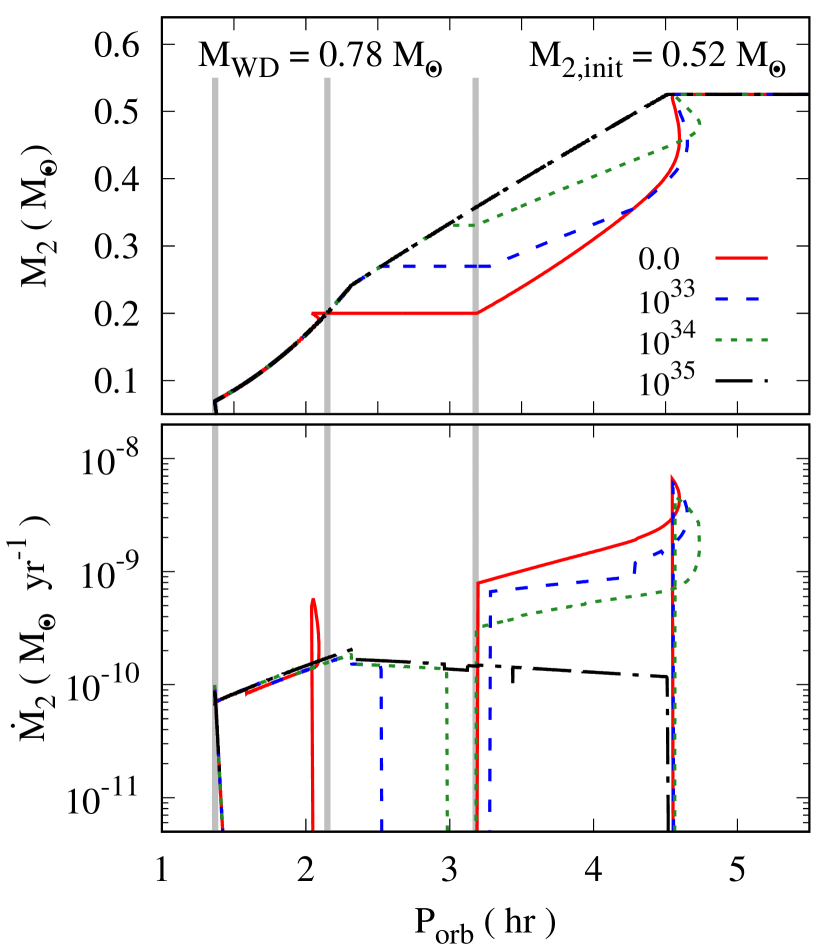
Figure 6: Evolution with orbital period ($P_{\rm orb}$) of donor mass ($M_{2}$, top panel), and mass transfer rate ($\dot{M}_{2}$, bottom panel). We show the evolution of one illustrative CV with initial donor and WD masses of 0.52 and 0.78 M_⊙, respectively, considering four values of $\mu_{\rm WD}$, in units of G cm³: 0.0 (red solid line), $10^{33}$ (long dashed blue line), $10^{34}$ (short dashed green line) and $10^{35}$ (dash-dotted black line). We also show in the plots the observational location of the period minimum (Gänsicke et al., 2009) and gap edges (Knigge, 2006), as vertical gray lines. Note that our CV evolution is in good agreement with WW02.

As described in Section 2, in polars, the WD magnetic field can close field lines from the donor, reducing in turn the wind zone, and consecutively diminishing wind-driven AML (i.e. MB). The effect of increasing $\mu_{\rm WD}$ on CV evolution is also shown in Fig. 6. As the MB efficiency becomes smaller with increasing $\mu_{\rm WD}$, mass transfer rates above the period gap also becomes smaller, and the donor star is driven less out of thermal equilibrium. As the donor is therefore less bloated, its contraction when MB is disrupted is less significant and the systems needs less time to become semidetached again. In other words, the lower edge of the gap is located at longer periods as the donor is more massive while entering the gap. As a consequence, the orbital period gap becomes partially/completely filled as $\mu_{\rm WD}$ increases. For sufficiently high values of $\mu_{\rm WD}$, MB is fully suppressed, and the system evolves as an accreting system through the period gap.

Comparing our results with those from WW02, we find a good agreement. Indeed, in both cases, the orbital period gap phase starts at roughly the same period for all values of $\mu_{\rm WD}$ ($\sim 3$ h), the gap width is consistently reduced for larger $\mu_{\rm WD}$ and the lower edge of the gap is located at longer orbital periods. In fact, as $\mu_{\rm WD}$ becomes greater, the MB efficiency becomes smaller, the mass transfer rate decreases, and consequentially the donor is less bloated. Given that our evolutionary tracks of polars resemble those of WW02, we can conclude that we successfully incorporated polar evolution in bse.

Appendix B Orbital Period and Distances for the SDSS systems

Table 2 presents our SDSS CV sample. It is composed of systems with reliably determined orbital periods from the literature.

Table 2: CVs from SDSS with reliable orbital period measurements. Distances are from Bailer-Jones et al. (2018) and have been derived from Gaia Data Release 2 parallax measurements (Gaia Collaboration et al., 2016, 2018). CVs are separated into four types, namely ‘NON-MAG’ (non-magnetic CVs), ‘POLAR’ (polars), ‘IP’ (intermediate polars) and ‘CV’ (unknown CV type).

SDSSJ $P_{\rm orb}$ (min) Distance (pc) Type Reference^a SDSSJ $P_{\rm orb}$ (min) Distance (pc) Type Reference^a 001153.08$-$064739.2 144.4 $506.8^{+38.4}_{-33.5}$ NON-MAG $(1)$ 091945.10$+$085710.0 81.3 $190.7^{+9.5}_{-8.6}$ NON-MAG $(36)$ 001538.25$+$263656.7 146.2 $602.6^{+79.0}_{-62.9}$ NON-MAG $(2)$ 092009.54$+$004244.8 212.9 $1559.6^{+627.9}_{-397.7}$ NON-MAG $(13)$ 001856.93$+$345444.2 855.0 $2050.9^{+418.7}_{-307.6}$ CV $(108)$ 092122.84$+$203857.1 84.2 ^b POLAR $(13)$ 002728.01$-$010828.5 85.4 ^b NON-MAG $(8)$ 092229.26$+$330743.6 89.1 $569.3^{+221.0}_{-128.6}$ NON-MAG $(117)$ 003640.29$+$230831.3 95.8 $634.7^{+120.9}_{-88.5}$ NON-MAG $(2)$ 092444.48$+$080150.9 131.2 $616.3^{+285.0}_{-154.9}$ CV $(15)$ 003827.04$+$250925.0 136.1 $478.5^{+97.8}_{-70.0}$ NON-MAG $(3)$ 093214.82$+$495054.7 602.5 $2236.1^{+320.6}_{-254.8}$ NON-MAG $(13)$ 003941.06$+$005427.5 91.4 $977.8^{+693.6}_{-425.6}$ NON-MAG $(4)$ 093249.57$+$472523.0 95.3 $795.3^{+288.9}_{-175.6}$ NON-MAG $(37)$ 004335.13$-$003729.8 82.3 $345.4^{+101.6}_{-64.6}$ NON-MAG $(5)$ 093537.46$+$161950.8 92.2 $1292.9^{+567.4}_{-351.6}$ CV $(43)$ 005050.87$+$000912.7 80.3 ^b NON-MAG $(6)$ 093836.98$+$071455.1 269.0 $499.7^{+51.2}_{-42.7}$ NON-MAG $(38)$ 013132.38$-$090122.2 81.5 $301.2^{+25.6}_{-21.9}$ NON-MAG $(6)$ 094325.90$+$520128.8 94.6 $798.6^{+221.5}_{-146.6}$ NON-MAG $(114)$ 013701.06$-$091234.8 79.7 $279.1^{+19.2}_{-16.9}$ NON-MAG $(7)$ 094431.70$+$035805.5 214.8 ^b NON-MAG $(109)$ 015151.86$+$140047.1 118.7 $665.2^{+443.3}_{-215.4}$ NON-MAG $(8)$ 094558.24$+$292252.2 92.0 $459.9^{+133.9}_{-86.0}$ POLAR $(43)$ 015543.39$+$002807.1 87.1 $317.2^{+14.6}_{-13.4}$ POLAR $(96)$ 094636.59$+$444644.7 123.6 $386.5^{+65.0}_{-49.0}$ NON-MAG $(39)$ 023322.60$+$005059.5 96.1 $614.4^{+438.7}_{-206.5}$ CV $(34)$ 100515.38$+$191107.9 107.6 $388.3^{+41.9}_{-34.6}$ NON-MAG $(13)$ 032855.00$+$052254.1 122.1 $579.6^{+324.8}_{-163.5}$ POLAR $(77)$ 100658.40$+$233724.4 267.7 $772.7^{+217.4}_{-143.1}$ NON-MAG $(40)$ 033449.86$-$071047.8 104.0 $428.9^{+66.8}_{-51.3}$ NON-MAG $(9)$ 101323.64$+$455858.9 118.1 $695.6^{+263.1}_{-156.3}$ NON-MAG $(36)$ 040714.78$-$064425.1 245.0 $659.0^{+41.7}_{-37.1}$ NON-MAG $(10)$ 101534.65$+$090441.9 79.9 $262.4^{+12.7}_{-11.6}$ POLAR $(79)$ 072910.68$+$365838.2 150.0 $844.7^{+709.3}_{-320.9}$ POLAR $(16)$ 101947.26$+$335753.6 92.7 $715.7^{+169.8}_{-117.4}$ NON-MAG $(41)$ 073208.11$+$413008.7 110.9 ^b NON-MAG $(76)$ 102026.48$+$530433.1 97.9 $365.3^{+15.7}_{-14.5}$ NON-MAG $(42)$ 073817.74$+$285519.6 127.0 $767.4^{+308.9}_{-177.2}$ NON-MAG $(11)$ 102320.27$+$440509.8 97.8 $631.2^{+159.0}_{-107.7}$ NON-MAG $(43)$ 074531.91$+$453829.3 79.5 $375.9^{+69.9}_{-51.2}$ NON-MAG $(12)$ 102637.04$+$475426.4 96.0 $566.9^{+357.4}_{-171.2}$ NON-MAG $(44)$ 074640.62$+$173412.8 93.5 $952.0^{+867.4}_{-416.0}$ NON-MAG $(13)$ 102800.08$+$214813.5 210.3 $1047.5^{+190.6}_{-142.1}$ NON-MAG $(36)$ 074813.54$+$290509.0 150.0 $1732.0^{+861.1}_{-554.8}$ NON-MAG $(14)$ 102905.21$+$485515.2 91.3 $143.3^{+5.1}_{-4.8}$ NON-MAG $(2)$ 075059.97$+$141150.1 134.2 $760.8^{+231.5}_{-146.9}$ NON-MAG $(15)$ 103147.99$+$085224.3 131.3 $1130.0^{+324.0}_{-215.2}$ NON-MAG $(115)$ 075117.09$+$144423.5 311.6 $841.9^{+181.0}_{-128.3}$ IP $(98)$ 103533.03$+$055158.4 82.1 $209.2^{+15.6}_{-13.6}$ NON-MAG $(45)$ 075240.44$+$362823.2 164.4 $497.5^{+626.0}_{-207.1}$ POLAR $(16)$ 104051.24$+$151133.7 337.7 $1358.7^{+212.7}_{-164.6}$ CV $(102)$ 075443.00$+$500729.2 206.0 $1448.0^{+420.1}_{-280.7}$ NON-MAG $(6)$ 104356.65$+$580731.5 106.4 $177.7^{+3.3}_{-3.2}$ NON-MAG $(46)$ 075507.69$+$143547.4 84.8 $259.0^{+18.2}_{-16.0}$ NON-MAG $(13)$ 105135.09$+$540435.6 114.5 $710.1^{+178.2}_{-121.1}$ POLAR $(80)$ 075653.11$+$085831.8 197.3 $1150.8^{+138.0}_{-112.0}$ NON-MAG $(17)$ 105430.43$+$300610.1 96.7 $322.0^{+12.6}_{-11.7}$ NON-MAG $(47)$ 075853.03$+$161645.1 86.1 $207.6^{+2.5}_{-2.5}$ IP $(99)$ 105550.08$+$095620.4 233.9 $877.7^{+147.7}_{-111.9}$ NON-MAG $(2)$ 075939.78$+$191417.2 188.4 $1228.8^{+367.0}_{-239.2}$ CV $(13)$ 105656.96$+$494118.3 100.2 $311.8^{+13.8}_{-12.7}$ NON-MAG $(48)$ 080215.39$+$401047.1 221.6 $1228.8^{+127.5}_{-106.3}$ NON-MAG $(13)$ 105754.25$+$275947.5 90.4 $620.1^{+372.5}_{-183.3}$ NON-MAG $(43)$ 080303.90$+$251627.0 102.0 $938.7^{+512.0}_{-271.2}$ NON-MAG $(18)$ 110014.72$+$131552.1 94.5 $460.3^{+77.0}_{-58.1}$ NON-MAG $(13)$ 080434.13$+$510349.2 85.0 $145.2^{+3.3}_{-3.2}$ NON-MAG $(19)$ 110425.64$+$450313.9 114.8 $320.3^{+14.8}_{-13.6}$ POLAR $(81)$ 080534.49$+$072029.1 329.3 $1663.5^{+570.8}_{-363.8}$ NON-MAG $(49)$ 110539.76$+$250628.6 113.9 $112.8^{+1.1}_{-1.1}$ POLAR $(82)$ 080846.19$+$313106.0 296.4 $1629.5^{+666.1}_{-424.6}$ NON-MAG $(13)$ 111126.82$+$571238.9 55.4 $568.9^{+46.2}_{-39.9}$ NON-MAG $(111)$ 080908.39$+$381406.2 193.0 $1222.2^{+77.6}_{-69.1}$ NON-MAG $(20)$ 111544.50$+$425822.4 115.9 $101.0^{+1.3}_{-1.2}$ POLAR $(50)$ 081207.63$+$131824.4 116.8 $1150.4^{+793.7}_{-442.1}$ NON-MAG $(13)$ 111721.92$+$520501.0 1636.7 $1735.5^{+655.2}_{-440.7}$ CV $(101)$ 081256.85$+$191157.8 230.6 $751.8^{+41.9}_{-37.8}$ NON-MAG $(21)$ 112003.39$+$663632.4 98.4 ^b NON-MAG $(116)$ 081321.91$+$452809.3 416.2 $1544.4^{+383.5}_{-267.9}$ NON-MAG $(22)$ 112253.32$-$111037.5 65.2 $811.2^{+731.5}_{-337.0}$ NON-MAG $(112)$ 081352.02$+$281317.2 175.1 $1190.0^{+352.0}_{-231.4}$ NON-MAG $(13)$ 113122.39$+$432238.5 91.1 $338.7^{+21.0}_{-18.7}$ NON-MAG $(36)$ 081610.83$+$453010.1 301.8 $974.8^{+605.4}_{-326.4}$ NON-MAG $(23)$ 113215.50$+$624900.4 99.2 $947.9^{+208.7}_{-148.0}$ NON-MAG $(36)$ 082051.06$+$493432.1 99.4 $891.0^{+603.0}_{-314.0}$ POLAR $(78)$ 113722.20$+$014858.7 109.6 $280.8^{+21.9}_{-19.0}$ NON-MAG $(42)$ 082236.05$+$510524.5 224.5 $765.9^{+31.5}_{-29.2}$ NON-MAG $(24)$ 113826.82$+$032207.0 84.7 $127.5^{+1.1}_{-1.1}$ NON-MAG $(51)$ 082409.72$+$493124.4 95.0 $1056.4^{+697.6}_{-403.1}$ NON-MAG $(8)$ 113950.57$+$455817.7 121.4 $540.3^{+231.5}_{-129.0}$ NON-MAG $(44)$ 083619.14$+$212105.3 105.6 $525.0^{+84.9}_{-64.6}$ NON-MAG $(25)$ 114955.68$+$284507.2 90.1 $331.5^{+38.8}_{-31.5}$ POLAR $(83)$ 083642.74$+$532838.0 81.8 $161.9^{+2.2}_{-2.1}$ NON-MAG $(26)$ 115207.00$+$404947.6 97.5 $739.1^{+521.8}_{-254.4}$ NON-MAG $(31)$ 083845.23$+$491055.5 99.7 $751.1^{+164.7}_{-116.4}$ NON-MAG $(13)$ 115215.80$+$491441.7 90.2 $318.5^{+19.8}_{-17.7}$ NON-MAG $(42)$ 083931.35$+$282824.0 109.0 $600.9^{+607.0}_{-252.5}$ NON-MAG $(27)$ 121209.31$+$013627.7 88.4 $149.2^{+4.1}_{-3.9}$ POLAR $(84)$ 084303.98$+$275149.6 84.6 $183.7^{+11.2}_{-10.0}$ NON-MAG $(28)$ 121607.03$+$052013.9 98.8 $448.1^{+531.3}_{-169.9}$ NON-MAG $(34)$ 084400.10$+$023919.3 298.1 $894.4^{+230.7}_{-155.7}$ NON-MAG $(13)$ 121913.04$+$204938.3 85.5 $281.8^{+36.3}_{-28.9}$ NON-MAG $(113)$ 084617.12$+$245344.1 263.2 $1315.6^{+581.9}_{-356.2}$ CV $(101)$ 122740.83$+$513924.9 90.6 $362.4^{+29.2}_{-25.2}$ NON-MAG $(52)$ 085107.38$+$030834.3 93.9 $707.8^{+172.5}_{-117.8}$ NON-MAG $(13)$ 123813.73$-$033932.9 80.5 $168.6^{+4.6}_{-4.3}$ NON-MAG $(53)$ 085344.17$+$574840.6 97.8 $151.9^{+1.5}_{-1.5}$ NON-MAG $(29)$ 123931.98$+$210806.2 125.3 $219.4^{+3.9}_{-3.8}$ NON-MAG $(33)$ 085414.02$+$390537.2 113.3 $553.0^{+163.9}_{-104.9}$ POLAR $(8)$ 124417.87$+$300400.8 111.5 $643.8^{+363.2}_{-180.0}$ NON-MAG $(36)$ 085521.17$+$111815.3 93.7 $586.8^{+75.2}_{-60.2}$ NON-MAG $(30)$ 124426.25$+$613514.6 142.9 $680.5^{+87.7}_{-70.2}$ NON-MAG $(8)$ 085909.18$+$053654.5 143.8 $437.1^{+32.4}_{-28.3}$ POLAR $(13)$ 125023.79$+$665525.5 84.6 $463.2^{+36.4}_{-31.5}$ NON-MAG $(8)$ 090016.55$+$430118.1 301.5 $817.2^{+116.2}_{-91.3}$ NON-MAG $(13)$ 125044.42$+$154957.3 86.3 $128.0^{+3.0}_{-2.9}$ POLAR $(85)$ 090103.93$+$480911.1 112.1 $563.3^{+299.1}_{-152.8}$ NON-MAG $(8)$ 125637.10$+$263643.2 94.8 $377.6^{+38.5}_{-32.1}$ NON-MAG $(54)$ 090350.72$+$330036.1 85.1 $400.3^{+77.8}_{-56.4}$ NON-MAG $(31)$ 130753.86$+$535130.5 79.7 $649.4^{+53.6}_{-46.1}$ POLAR $(86)$ 090403.48$+$035501.2 86.0 $277.7^{+77.0}_{-49.8}$ NON-MAG $(32)$ 131223.48$+$173659.1 91.9 $574.6^{+354.6}_{-165.1}$ POLAR $(87)$ 090628.25$+$052656.9 215.6 $937.5^{+251.5}_{-168.3}$ NON-MAG $(113)$ 132411.57$+$032050.5 158.7 ^b POLAR $(43)$ 090950.53$+$184947.4 252.6 $262.0^{+4.8}_{-4.6}$ NON-MAG $(33)$ 132723.38$+$652854.2 196.8 $1570.3^{+468.6}_{-314.3}$ NON-MAG $(55)$ 091127.36$+$084140.7 295.7 $964.5^{+547.1}_{-296.8}$ NON-MAG $(34)$ 133309.19$+$143706.9 132.0 $1634.9^{+994.7}_{-630.9}$ POLAR $(88)$ 091216.20$+$505353.8 78.6 $673.6^{+38.2}_{-34.4}$ NON-MAG $(35)$ 133940.98$+$484727.9 82.5 $149.5^{+2.0}_{-1.9}$ NON-MAG $(56)$ 091242.18$+$620940.1 115.4 $300.4^{+42.0}_{-33.0}$ NON-MAG $(36)$ 134323.16$+$150916.8 92.7 $393.7^{+27.7}_{-24.3}$ NON-MAG $(41)$ 091650.76$+$284943.1 265.7 $983.3^{+595.2}_{-336.7}$ NON-MAG $(36)$ 143317.78$+$101123.3 78.1 $223.8^{+10.7}_{-9.8}$ NON-MAG $(52)$

Table 2 – continued.

SDSSJ $P_{\rm orb}$ (min) Distance (pc) Type Reference^a SDSSJ $P_{\rm orb}$ (min) Distance (pc) Type Reference^a 143500.22$-$004606.3 104.7 $558.7^{+205.5}_{-119.3}$ NON-MAG $(57)$ 163722.21$-$001957.1 97.0 $2504.0^{+2592.3}_{-1367.4}$ NON-MAG $(5)$ 145758.21$+$514807.9 77.9 $585.2^{+146.8}_{-99.0}$ NON-MAG $(58)$ 164248.52$+$134751.4 113.6 $533.8^{+36.0}_{-31.8}$ NON-MAG $(5)$ 150137.22$+$550123.4 81.9 $342.1^{+37.3}_{-30.7}$ NON-MAG $(31)$ 165359.05$+$201010.4 90.9 $899.9^{+173.1}_{-125.8}$ NON-MAG $(36)$ 150240.97$+$333423.8 84.8 $185.8^{+3.1}_{-3.0}$ NON-MAG $(31)$ 165658.12$+$212139.3 97.0 $523.7^{+47.3}_{-40.2}$ NON-MAG $(36)$ 150441.76$+$084752.6 116.5 $1061.6^{+642.4}_{-306.8}$ NON-MAG $(36)$ 165837.70$+$184727.4 98.0 $415.1^{+82.6}_{-59.3}$ NON-MAG $(5)$ 150722.15$+$523040.2 66.6 $210.1^{+6.5}_{-6.1}$ NON-MAG $(52)$ 165951.69$+$192745.6 203.0 $1573.3^{+224.1}_{-175.6}$ NON-MAG $(36)$ 151302.29$+$231508.4 140.4 $756.7^{+30.8}_{-28.5}$ NON-MAG $(42)$ 170053.29$+$400357.6 116.4 $524.1^{+34.2}_{-30.3}$ POLAR $(16)$ 151415.65$+$074446.4 88.7 $181.1^{+7.9}_{-7.2}$ POLAR $(85)$ 170213.25$+$322954.1 114.1 $292.3^{+11.3}_{-10.5}$ NON-MAG $(70)$ 152419.33$+$220920.0 93.6 $469.2^{+79.5}_{-59.6}$ NON-MAG $(15)$ 171145.08$+$301319.9 80.3 $364.1^{+101.9}_{-65.5}$ NON-MAG $(8)$ 152613.96$+$081802.3 107.4 $378.3^{+43.6}_{-35.5}$ NON-MAG $(59)$ 173008.38$+$624754.7 110.3 $528.5^{+10.8}_{-10.4}$ NON-MAG $(36)$ 153634.42$+$332851.9 132.6 $819.0^{+244.4}_{-155.8}$ NON-MAG $(36)$ 173102.22$+$342633.2 300.2 $2112.2^{+893.9}_{-529.3}$ NON-MAG $(2)$ 153817.35$+$512338.0 93.1 $622.2^{+73.4}_{-59.6}$ NON-MAG $(8)$ 204448.92$-$045928.8 2420.0 $2016.9^{+517.3}_{-349.9}$ NON-MAG $(71)$ 154104.67$+$360252.8 84.3 $414.4^{+16.9}_{-15.6}$ POLAR $(13)$ 204720.76$+$000007.7 89.0 $478.9^{+259.3}_{-124.9}$ NON-MAG $(115)$ 154453.60$+$255348.8 361.8 $519.6^{+21.4}_{-19.8}$ NON-MAG $(60)$ 204817.85$-$061044.8 87.3 $608.6^{+370.5}_{-168.5}$ NON-MAG $(72)$ 154539.08$+$142231.4 280.8 $3452.5^{+862.7}_{-604.6}$ NON-MAG $(61)$ 204827.91$+$005008.9 252.0 $591.8^{+74.5}_{-59.7}$ POLAR $(93)$ 155247.18$+$185629.1 113.5 $131.3^{+0.8}_{-0.8}$ POLAR $(89)$ 205017.83$-$053626.8 94.2 ^b POLAR $(97)$ 155331.11$+$551614.4 263.5 $185.3^{+3.3}_{-3.2}$ POLAR $(90)$ 205914.87$-$061220.4 107.5 $2031.9^{+1495.5}_{-783.0}$ NON-MAG $(6)$ 155412.33$+$272152.4 151.9 $207.6^{+3.2}_{-3.1}$ POLAR $(91)$ 210014.11$+$004445.9 120.0 $928.0^{+131.9}_{-103.2}$ NON-MAG $(73)$ 155531.98$-$001054.9 113.5 $648.5^{+190.8}_{-120.7}$ NON-MAG $(6)$ 210449.94$+$010545.8 103.6 $1999.3^{+1515.9}_{-927.1}$ NON-MAG $(6)$ 155644.23$-$000950.2 115.4 $308.2^{+22.1}_{-19.4}$ NON-MAG $(36)$ 211605.42$+$113407.4 80.2 ^b NON-MAG $(8)$ 155654.47$+$210718.9 119.8 $319.3^{+10.0}_{-9.4}$ NON-MAG $(62)$ 214140.43$+$050729.9 76.0 $257.3^{+39.1}_{-30.1}$ NON-MAG $(74)$ 155656.92$+$352336.6 126.9 $1377.5^{+491.1}_{-301.9}$ NON-MAG $(63)$ 215411.12$-$090121.6 319.0 ^b CV $(8)$ 160745.02$+$362320.7 225.4 $1815.9^{+764.1}_{-465.5}$ NON-MAG $(13)$ 220553.98$+$115553.7 82.8 $871.3^{+878.8}_{-357.5}$ NON-MAG $(75)$ 161007.50$+$035232.7 190.5 $323.3^{+11.8}_{-11.0}$ POLAR $(36)$ 221832.76$+$192520.2 129.5 $237.5^{+7.3}_{-6.9}$ POLAR $(94)$ 161027.61$+$090738.4 81.9 $400.8^{+132.9}_{-80.0}$ NON-MAG $(64)$ 223439.93$+$004127.2 127.3 $494.8^{+44.5}_{-37.8}$ NON-MAG $(13)$ 161033.63$-$010223.2 80.5 $242.5^{+25.0}_{-20.8}$ NON-MAG $(65)$ 223843.83$+$010820.6 194.3 $2172.8^{+866.4}_{-571.9}$ IP $(5)$ 161909.10$+$135145.5 412.6 $1671.8^{+301.7}_{-224.1}$ NON-MAG $(36)$ 224736.37$+$250436.3 81.6 ^b NON-MAG $(110)$ 161935.76$+$524631.8 100.5 $438.5^{+50.7}_{-41.3}$ POLAR $(92)$ 225831.18$-$094931.7 118.9 $294.0^{+5.0}_{-4.8}$ NON-MAG $(9)$ 162501.74$+$390926.3 78.7 $291.5^{+8.6}_{-8.1}$ NON-MAG $(66)$ 230351.64$+$010651.0 110.5 $635.8^{+230.4}_{-136.9}$ NON-MAG $(13)$ 162520.29$+$120308.7 138.2 $457.2^{+58.0}_{-46.4}$ NON-MAG $(67)$ 230949.12$+$213516.7 255.8 $172.1^{+1.9}_{-1.8}$ CV $(103)$ 162718.38$+$120434.9 150.0 $1152.6^{+512.1}_{-277.8}$ NON-MAG $(68)$ 231930.43$+$261518.6 180.6 $516.2^{+27.7}_{-25.1}$ POLAR $(95)$ 162936.53$+$263519.5 134.0 $683.9^{+124.5}_{-91.8}$ POLAR $(13)$ 233325.92$+$152222.1 83.1 $745.8^{+239.7}_{-150.0}$ IP $(100)$ 163545.72$+$112458.0 189.0 $1037.8^{+45.9}_{-42.3}$ NON-MAG $(69)$ a References: (1) Rebassa-Mansergas et al. (2014), (2) Thorstensen et al. (2016), (3) Pavlenko et al. (2016), (4) Southworth et al. (2010b), (5) Southworth et al. (2008b), (6) Southworth et al. (2007b), (7) Pretorius et al. (2004), (8) Dillon et al. (2008), (9) Kato et al. (2009), (10) Ak et al. (2005), (11) Szkody et al. (2003a), (12) Mukadam et al. (2013), (13) Gänsicke et al. (2009), (14) Szkody et al. (2004), (15) Southworth et al. (2010a), (16) Homer et al. (2005), (17) Tovmassian et al. (2014), (18) Szkody et al. (2005), (19) Zharikov et al. (2008), (20) Rodríguez-Gil et al. (2007b), (21) Gülsecen & Esenog̃lu (2014), (22) Thorstensen et al. (2004), (23) Shears et al. (2012), (24) Stanishev et al. (2006), (25) Thorstensen (1997), (26) Howell & Szkody (1988), (27) Kato et al. (2014), (29) Ringwald et al. (1994), (30) Arenas & Mennickent (1998), (31) Savoury et al. (2011), (32) Woudt et al. (2005), (33) Feline et al. (2005), (34) Southworth et al. (2006), (35) Rutkowski et al. (2009), (36) Thorstensen et al. (2015), (37) Homer et al. (2006), (38) Thorstensen & Taylor (2001), (39) Feline et al. (2004b), (40) Southworth et al. (2009), (41) Aungwerojwit et al. (2006), (42) Patterson et al. (2003), (43) Southworth et al. (2015), (44) Breedt et al. (2014), (45) Littlefair et al. (2006), (46) Steeghs et al. (2003), (47) Wagner et al. (1998), (48) Thorstensen et al. (1996), (49) Woudt et al. (2012), (50) Schmidt et al. (1999), (51) Shafter & Szkody (1984), (52) Littlefair et al. (2008), (53) Pala et al. (2019b), (54) Howell et al. (1995a), (55) Wolfe et al. (2003), (56) Gänsicke et al. (2006), (57) Feline et al. (2004a), (58) Uthas et al. (2012), (59) Olech et al. (2003), (60) Skinner et al. (2011), (61) Ringwald et al. (2005), (62) Thorstensen et al. (2002b), (63) Hardy et al. (2017), (64) Kato (2015), (65) Woudt & Warner (2004), (66) Thorstensen et al. (2002a), (67) Olech et al. (2011), (68) Shears et al. (2009), (69) Rodríguez-Gil et al. (2007a), (70) Khruzina et al. (2015), (71) Peters & Thorstensen (2005), (72) Woudt & Warner (2010), (73) Olech et al. (2009), (74) Szkody et al. (2014), (75) Southworth et al. (2008a), (76) Shears et al. (2011), (77) Babina et al. (2017), (78) Schwope et al. (2002b), (79) Burwitz et al. (1998), (80) Morris et al. (1987), (81) Bonnet-Bidaud et al. (1996), (82) Cropper (1986), (83) Howell et al. (1995b), (84) Burleigh et al. (2006), (85) Breedt et al. (2012a), (86) Katajainen et al. (2000), (87) Vogel et al. (2008), (88) Schmidt et al. (2008), (89) Schwope et al. (1991), (90) Szkody et al. (2003b), (91) Thorstensen & Fenton (2002), (92) Denisenko & Martinelli (2016), (93) Schmidt et al. (2005), (94) Thorstensen & Halpern (2013), (95) Shafter et al. (2008), (96) Woudt et al. (2004), (97) Potter et al. (2006), (98) Evans et al. (2006), (99) Rodríguez-Gil et al. (2004), (100) Southworth et al. (2007a), (101) Drake et al. (2014), (102) Abbott et al. (1990), (103) Thorstensen et al. (2009), (104) Hilton et al. (2009), (105) Thorstensen & Armstrong (2005), (106) Reimers et al. (1999), (107) Schmidt et al. (2007), (108) González-Buitrago et al. (2013), (109) Mennickent et al. (2002), (110) Kato et al. (2013), (111) Kennedy et al. (2015), (112) Breedt et al. (2012b), (113) Schmidtobreick (private communication), (114) Thorstensen (private communication), (115) Breedt (private communication), (116) Stein (private communication), (117) Southworth (private communication). b There is no parallax measurement in Gaia DR2.

References

- Abbott et al. (1990) Abbott T. M. C., Shafter A. W., Wood J. H., Tomaney A. B., Haswell C. A., 1990, PASP, 102, 558
- Ak et al. (2005) Ak T., Retter A., Liu A., Esenoğlu H. H., 2005, Publ. Astron. Soc. Australia, 22, 105
- Althaus & Benvenuto (1997) Althaus L. G., Benvenuto O. G., 1997, ApJ, 477, 313
- Angel et al. (1981) Angel J. R. P., Borra E. F., Landstreet J. D., 1981, ApJS, 45, 457
- Araujo-Betancor & et al. (2005) Araujo-Betancor S., et al. 2005, ApJ, 622, 589
- Arenas & Mennickent (1998) Arenas J., Mennickent R. E., 1998, A&A, 337, 472
- Aungwerojwit et al. (2006) Aungwerojwit A., et al., 2006, A&A, 455, 659
- Babina et al. (2017) Babina J. V., Pavlenko E. P., Antonyuk O. I., 2017, Astrophysics, 60, 28
- Bailer-Jones et al. (2018) Bailer-Jones C. A. L., Rybizki J., Fouesneau M., Mantelet G., Andrae R., 2018, AJ, 156, 58
- Belloni & Schreiber (2019) Belloni D., Schreiber M. R., 2019, arXiv e-prints, p. arXiv:1910.08582
- Belloni et al. (2018) Belloni D., Schreiber M. R., Zorotovic M., Iłkiewicz K., Hurley J. R., Giersz M., Lagos F., 2018, MNRAS, 478, 5639
- Belloni et al. (2019) Belloni D., Giersz M., Rivera Sandoval L. E., Askar A., Ciecielåg P., 2019, MNRAS, 483, 315
- Bonnet-Bidaud et al. (1996) Bonnet-Bidaud J. M., Mouchet M., Somova T. A., Somov N. N., 1996, A&A, 306, 199
- Breedt et al. (2012a) Breedt E., Gänsicke B. T., Girven J., Drake A. J., Copperwheat C. M., Parsons S. G., Marsh T. R., 2012a, MNRAS, 423, 1437
- Breedt et al. (2012b) Breedt E., Gänsicke B. T., Marsh T. R., Steeghs D., Drake A. J., Copperwheat C. M., 2012b, MNRAS, 425, 2548
- Breedt et al. (2014) Breedt E., et al., 2014, MNRAS, 443, 3174
- Burleigh et al. (2006) Burleigh M. R., et al., 2006, MNRAS, 373, 1416
- Burwitz et al. (1998) Burwitz V., et al., 1998, A&A, 331, 262
- Camacho et al. (2014) Camacho J., Torres S., García-Berro E., Zorotovic M., Schreiber M. R., Rebassa-Mansergas A., Nebot Gómez-Morán A., Gänsicke B. T., 2014, A&A, 566, A86
- Claeys et al. (2014) Claeys J. S. W., Pols O. R., Izzard R. G., Vink J., Verbunt F. W. M., 2014, A&A, 563, A83
- Cojocaru et al. (2017) Cojocaru R., Rebassa-Mansergas A., Torres S., García-Berro E., 2017, MNRAS, 470, 1442
- Cropper (1986) Cropper M., 1986, MNRAS, 222, 853
- Cropper (1990) Cropper M., 1990, Space Sci. Rev., 54, 195
- Davis et al. (2008) Davis P. J., Kolb U., Willems B., Gänsicke B. T., 2008, MNRAS, 389, 1563
- Denisenko & Martinelli (2016) Denisenko D. V., Martinelli F., 2016, arXiv e-prints,
- Dillon et al. (2008) Dillon M., et al., 2008, MNRAS, 386, 1568
- Drake et al. (2014) Drake A. J., et al., 2014, ApJS, 213, 9
- Evans et al. (2006) Evans P. A., Hellier C., Ramsay G., 2006, MNRAS, 369, 1229
- Feline et al. (2004a) Feline W. J., Dhillon V. S., Marsh T. R., Stevenson M. J., Watson C. A., Brinkworth C. S., 2004a, MNRAS, 347, 1173
- Feline et al. (2004b) Feline W. J., Dhillon V. S., Marsh T. R., Brinkworth C. S., 2004b, MNRAS, 355, 1
- Feline et al. (2005) Feline W. J., Dhillon V. S., Marsh T. R., Watson C. A., Littlefair S. P., 2005, MNRAS, 364, 1158
- Ferrario et al. (2015) Ferrario L., de Martino D., Gänsicke B. T., 2015, Space Sci. Rev., 191, 111
- Fontaine et al. (2001) Fontaine G., Brassard P., Bergeron P., 2001, PASP, 113, 409
- Gaia Collaboration et al. (2016) Gaia Collaboration et al., 2016, A&A, 595, A1
- Gaia Collaboration et al. (2018) Gaia Collaboration et al., 2018, A&A, 616, A1
- Gänsicke et al. (2006) Gänsicke B. T., et al., 2006, MNRAS, 365, 969
- Gänsicke et al. (2009) Gänsicke B. T., et al., 2009, MNRAS, 397, 2170
- Goliasch & Nelson (2015) Goliasch J., Nelson L., 2015, ApJ, 809, 80
- González-Buitrago et al. (2013) González-Buitrago D., Tovmassian G., Zharikov S., Yungelson L., Miyaji T., Echevarría J., Aviles A., Valyavin G., 2013, A&A, 553, A28
- Gülsecen & Esenog̃lu (2014) Gülsecen H., Esenog̃lu H., 2014, New Astron., 28, 49
- Hameury et al. (1989) Hameury J. M., King A. R., Lasota J. P., 1989, MNRAS, 237, 845
- Hardy et al. (2017) Hardy L. K., et al., 2017, MNRAS, 465, 4968
- Hellier (2001) Hellier C., 2001, Cataclysmic Variable Stars. Springer, New York
- Hernández Santisteban et al. (2018) Hernández Santisteban J. V., Knigge C., Pretorius M. L., Sullivan M., Warner B., 2018, MNRAS, 473, 3241
- Hilton et al. (2009) Hilton E. J., Szkody P., Mukadam A., Henden A., Dillon W., Schmidt G. D., 2009, AJ, 137, 3606
- Holberg et al. (2008) Holberg J. B., Sion E. M., Oswalt T., McCook G. P., Foran S., Subasavage J. P., 2008, AJ, 135, 1225
- Holberg et al. (2016) Holberg J. B., Oswalt T. D., Sion E. M., McCook G. P., 2016, MNRAS, 462, 2295
- Hollands et al. (2018) Hollands M. A., Tremblay P. E., Gänsicke B. T., Gentile-Fusillo N. P., Toonen S., 2018, MNRAS, 480, 3942
- Homer et al. (2005) Homer L., et al., 2005, ApJ, 620, 929
- Homer et al. (2006) Homer L., Szkody P., Chen B., Henden A., Schmidt G., Anderson S. F., Silvestri N. M., Brinkmann J., 2006, AJ, 131, 562
- Howell & Szkody (1988) Howell S., Szkody P., 1988, PASP, 100, 224
- Howell et al. (1995a) Howell S. B., Szkody P., Cannizzo J. K., 1995a, ApJ, 439, 337
- Howell et al. (1995b) Howell S. B., Sirk M. M., Malina R. F., Mittaz J. P. D., Mason K. O., 1995b, ApJ, 439, 991
- Howell et al. (2001) Howell S. B., Nelson L. A., Rappaport S., 2001, ApJ, 550, 897
- Hurley et al. (2000) Hurley J. R., Pols O. R., Tout C. A., 2000, MNRAS, 315, 543
- Hurley et al. (2002) Hurley J. R., Tout C. A., Pols O. R., 2002, MNRAS, 329, 897
- Isern et al. (2017) Isern J., García-Berro E., Külebi B., Lorén-Aguilar P., 2017, ApJ, 836, L28
- Jiménez-Esteban et al. (2018) Jiménez-Esteban F. M., Torres S., Rebassa-Mansergas A., Skorobogatov G., Solano E., Cantero C., Rodrigo C., 2018, MNRAS, 480, 4505
- Kalomeni et al. (2016) Kalomeni B., Nelson L., Rappaport S., Molnar M., Quintin J., Yakut K., 2016, ApJ, 833, 83
- Katajainen et al. (2000) Katajainen S., Lehto H. J., Piirola V., Karttunen H., Piironen J., 2000, A&A, 357, 677
- Kato (2015) Kato T., 2015, PASJ, 67, 108
- Kato et al. (2009) Kato T., et al., 2009, PASJ, 61, S395
- Kato et al. (2013) Kato T., et al., 2013, PASJ, 65, 23
- Kato et al. (2014) Kato T., et al., 2014, PASJ, 66, 30
- Kawka et al. (2007) Kawka A., Vennes S., Schmidt G. D., Wickramasinghe D. T., Koch R., 2007, ApJ, 654, 499
- Kennedy et al. (2015) Kennedy M., Garnavich P., Callanan P., Szkody P., Littlefield C., Pogge R., 2015, ApJ, 815, 131
- Khruzina et al. (2015) Khruzina T. S., Golysheva P. Y., Katysheva N. A., Shugarov S. Y., Shakura N. I., 2015, Astronomy Reports, 59, 288
- Kilic et al. (2017) Kilic M., Munn J. A., Harris H. C., von Hippel T., Liebert J. W., Williams K. A., Jeffery E., DeGennaro S., 2017, ApJ, 837, 162
- Knigge (2006) Knigge C., 2006, MNRAS, 373, 484
- Knigge et al. (2011) Knigge C., Baraffe I., Patterson J., 2011, ApJS, 194, 28
- Kolb (1993) Kolb U., 1993, A&A, 271, 149
- Kroupa (2001) Kroupa P., 2001, MNRAS, 322, 231
- Kroupa et al. (2013) Kroupa P., Weidner C., Pflamm-Altenburg J., Thies I., Dabringhausen J., Marks M., Maschberger T., 2013, The Stellar and Sub-Stellar Initial Mass Function of Simple and Composite Populations. in Oswalt T. D., Gilmore G., eds, Planets, Stars and Stellar Systems, Vol. 5. Springer, Netherlands, p. 115, doi:10.1007/978-94-007-5612-0˙4
- Li & Wickramasinghe (1998) Li J., Wickramasinghe D. T., 1998, MNRAS, 300, 718
- Li et al. (1994) Li J. K., Wu K. W., Wickramasinghe D. T., 1994, MNRAS, 268, 61
- Littlefair et al. (2006) Littlefair S. P., Dhillon V. S., Marsh T. R., Gänsicke B. T., Southworth J., Watson C. A., 2006, Science, 314, 1578
- Littlefair et al. (2008) Littlefair S. P., Dhillon V. S., Marsh T. R., Gänsicke B. T., Southworth J., Baraffe I., Watson C. A., Copperwheat C., 2008, MNRAS, 388, 1582
- McAllister et al. (2019) McAllister M., et al., 2019, MNRAS, 486, 5535
- Mennickent et al. (2002) Mennickent R. E., Tovmassian G., Zharikov S. V., Tappert C., Greiner J., Gänsicke B. T., Fried R. E., 2002, A&A, 383, 933
- Mestel (1968) Mestel L., 1968, MNRAS, 138, 359
- Mestel & Spruit (1987) Mestel L., Spruit H. C., 1987, MNRAS, 226, 57
- Morris et al. (1987) Morris S. L., Schmidt G. D., Liebert J., Stocke J., Gioia I. M., Maccacaro T., 1987, ApJ, 314, 641
- Mukadam et al. (2013) Mukadam A. S., et al., 2013, AJ, 146, 54
- Olech et al. (2003) Olech A., Kȩdzierski P., Złoczewski K., Mularczyk K., Wiśniewski M., 2003, A&A, 411, 483
- Olech et al. (2009) Olech A., Rutkowski A., Schwarzenberg-Czerny A., 2009, MNRAS, 399, 465
- Olech et al. (2011) Olech A., et al., 2011, A&A, 532, A64
- Paczyński (1967) Paczyński B., 1967, Acta Astron., 17, 287
- Pala et al. (2017) Pala A. F., et al., 2017, MNRAS, 466, 2855
- Pala et al. (2019a) Pala A. F., et al., 2019a, arXiv e-prints, p. arXiv:1907.13152
- Pala et al. (2019b) Pala A. F., et al., 2019b, MNRAS, 483, 1080
- Parsons et al. (2013) Parsons S. G., Marsh T. R., Gänsicke B. T., Schreiber M. R., Bours M. C. P., Dhillon V. S., Littlefair S. P., 2013, MNRAS, 436, 241
- Patience et al. (2002) Patience J., Ghez A. M., Reid I. N., Matthews K., 2002, AJ, 123, 1570
- Patterson (1994) Patterson J., 1994, PASP, 106, 209
- Patterson et al. (2003) Patterson J., et al., 2003, PASP, 115, 1308
- Pavlenko et al. (2016) Pavlenko E. P., Sosnovskij A. A., Katysheva N. A., Kato T., Littlefield K., 2016, Astrophysics, 59, 304
- Peters & Thorstensen (2005) Peters C. S., Thorstensen J. R., 2005, PASP, 117, 1386
- Politano (1996) Politano M., 1996, ApJ, 465, 338
- Potter et al. (2006) Potter S. B., O’Donoghue D., Romero-Colmenero E., Buckley D. A. H., Woudt P. A., Warner B., 2006, MNRAS, 371, 727
- Pretorius & Knigge (2012) Pretorius M. L., Knigge C., 2012, MNRAS, 419, 1442
- Pretorius et al. (2004) Pretorius M. L., Woudt P. A., Warner B., Bolt G., Patterson J., Armstrong E., 2004, MNRAS, 352, 1056
- Pretorius et al. (2013) Pretorius M. L., Knigge C., Schwope A. D., 2013, MNRAS, 432, 570
- Prialnik (1986) Prialnik D., 1986, ApJ, 310, 222
- Rappaport et al. (1982) Rappaport S., Joss P. C., Webbink R. F., 1982, ApJ, 254, 616
- Rappaport et al. (1983) Rappaport S., Verbunt F., Joss P. C., 1983, ApJ, 275, 713
- Rebassa-Mansergas et al. (2014) Rebassa-Mansergas A., Parsons S. G., Copperwheat C. M., Justham S., Gänsicke B. T., Schreiber M. R., Marsh T. R., Dhillon V. S., 2014, ApJ, 790, 28
- Recchi & Kroupa (2015) Recchi S., Kroupa P., 2015, MNRAS, 446, 4168
- Reimers & Hagen (2000) Reimers D., Hagen H.-J., 2000, A&A, 358, L45
- Reimers et al. (1999) Reimers D., Hagen H.-J., Hopp U., 1999, A&A, 343, 157
- Reiners & Basri (2009) Reiners A., Basri G., 2009, A&A, 496, 787
- Ringwald et al. (1994) Ringwald F. A., Thorstensen J. R., Hamwey R. M., 1994, MNRAS, 271, 323
- Ringwald et al. (2005) Ringwald F. A., Chase D. W., Reynolds D. S., 2005, PASP, 117, 1223
- Rodríguez-Gil et al. (2004) Rodríguez-Gil P., Gänsicke B. T., Araujo-Betancor S., Casares J., 2004, MNRAS, 349, 367
- Rodríguez-Gil et al. (2007a) Rodríguez-Gil P., Schmidtobreick L., Gänsicke B. T., 2007a, MNRAS, 374, 1359
- Rodríguez-Gil et al. (2007b) Rodríguez-Gil P., et al., 2007b, MNRAS, 377, 1747
- Rutkowski et al. (2009) Rutkowski A., Olech A., Wiśniewski M., Pietrukowicz P., Pala J., Poleski R., 2009, A&A, 497, 437
- Savoury et al. (2011) Savoury C. D. J., et al., 2011, MNRAS, 415, 2025
- Schatzman (1962) Schatzman E., 1962, Annales d’Astrophysique, 25, 18
- Schmidt et al. (1999) Schmidt G. D., Hoard D. W., Szkody P., Melia F., Honeycutt R. K., Wagner R. M., 1999, ApJ, 525, 407
- Schmidt et al. (2005) Schmidt G. D., et al., 2005, ApJ, 630, 1037
- Schmidt et al. (2007) Schmidt G. D., Szkody P., Henden A., Anderson S. F., Lamb D. Q., Margon B., Schneider D. P., 2007, ApJ, 654, 521
- Schmidt et al. (2008) Schmidt G. D., Smith P. S., Szkody P., Anderson S. F., 2008, PASP, 120, 160
- Schreiber & Gänsicke (2003) Schreiber M. R., Gänsicke B. T., 2003, A&A, 406, 305
- Schreiber et al. (2010) Schreiber M. R., et al., 2010, A&A, 513, L7
- Schreiber et al. (2016) Schreiber M. R., Zorotovic M., Wijnen T. P. G., 2016, MNRAS, 455, L16
- Schulz et al. (2015) Schulz C., Pflamm-Altenburg J., Kroupa P., 2015, A&A, 582, A93
- Schwope (2018) Schwope A. D., 2018, A&A, 619, A62
- Schwope et al. (1991) Schwope A. D., Thomas H. C., Beuermann K., Naundorf C. E., 1991, A&A, 244, 373
- Schwope et al. (2002a) Schwope A. D., Brunner H., Hambaryan V., Schwarz R., 2002a, in Gänsicke B. T., Beuermann K., Reinsch K., eds, Astronomical Society of the Pacific Conference Series Vol. 261, The Physics of Cataclysmic Variables and Related Objects. p. 102
- Schwope et al. (2002b) Schwope A. D., Brunner H., Buckley D., Greiner J., Heyden K. v. d., Neizvestny S., Potter S., Schwarz R., 2002b, A&A, 396, 895
- Schwope et al. (2009) Schwope A. D., Nebot Gomez-Moran A., Schreiber M. R., Gänsicke B. T., 2009, A&A, 500, 867
- Shafter & Szkody (1984) Shafter A. W., Szkody P., 1984, ApJ, 276, 305
- Shafter et al. (2008) Shafter A. W., Davenport J. R. A., Güth T., Kattner S., Marin E., Sreenivasamurthy N., 2008, PASP, 120, 374
- Shears et al. (2009) Shears J., Brady S., Gaensicke B., Krajci T., Miller I., Oegmen Y., Pietz J., Staels B., 2009, Journal of the British Astronomical Association, 119, 144
- Shears et al. (2011) Shears J., Koff R., Sabo R., Staels B., Stein W., Wils P., 2011, Journal of the British Astronomical Association, 121, 228
- Shears et al. (2012) Shears J., et al., 2012, Journal of the British Astronomical Association, 122, 237
- Skinner et al. (2011) Skinner J. N., Thorstensen J. R., Armstrong E., Brady S., 2011, PASP, 123, 259
- Southworth et al. (2006) Southworth J., Gänsicke B. T., Marsh T. R., de Martino D., Hakala P., Littlefair S., Rodríguez-Gil P., Szkody P., 2006, MNRAS, 373, 687
- Southworth et al. (2007a) Southworth J., Gänsicke B. T., Marsh T. R., de Martino D., Aungwerojwit A., 2007a, MNRAS, 378, 635
- Southworth et al. (2007b) Southworth J., Marsh T. R., Gänsicke B. T., Aungwerojwit A., Hakala P., de Martino D., Lehto H., 2007b, MNRAS, 382, 1145
- Southworth et al. (2008a) Southworth J., Townsley D. M., Gänsicke B. T., 2008a, MNRAS, 388, 709
- Southworth et al. (2008b) Southworth J., et al., 2008b, MNRAS, 391, 591
- Southworth et al. (2009) Southworth J., Hickman R. D. G., Marsh T. R., Rebassa-Mansergas A., Gänsicke B. T., Copperwheat C. M., Rodríguez-Gil P., 2009, A&A, 507, 929
- Southworth et al. (2010a) Southworth J., Copperwheat C. M., Gänsicke B. T., Pyrzas S., 2010a, A&A, 510, A100
- Southworth et al. (2010b) Southworth J., Marsh T. R., Gänsicke B. T., Steeghs D., Copperwheat C. M., 2010b, A&A, 524, A86
- Southworth et al. (2015) Southworth J., Tappert C., Gänsicke B. T., Copperwheat C. M., 2015, A&A, 573, A61
- Stanishev et al. (2006) Stanishev V., Kraicheva Z., Genkov V., 2006, A&A, 455, 223
- Steeghs et al. (2003) Steeghs D., Perryman M. A. C., Reynolds A., de Bruijne J. H. J., Marsh T., Dhillon V. S., Peacock A., 2003, MNRAS, 339, 810
- Szkody et al. (2003a) Szkody P., et al., 2003a, AJ, 126, 1499
- Szkody et al. (2003b) Szkody P., et al., 2003b, ApJ, 583, 902
- Szkody et al. (2004) Szkody P., et al., 2004, AJ, 128, 1882
- Szkody et al. (2005) Szkody P., et al., 2005, AJ, 129, 2386
- Szkody et al. (2014) Szkody P., Everett M. E., Howell S. B., Landolt A. U., Bond H. E., Silva D. R., Vasquez-Soltero S., 2014, AJ, 148, 63
- Tappert et al. (2017) Tappert C., Fuentes-Morales I., Puebla E., Ederoclite A., Schmidtobreick L., Vogt N., 2017, arXiv e-prints, p. arXiv:1702.02415
- Thorstensen (1997) Thorstensen J. R., 1997, PASP, 109, 1241
- Thorstensen & Armstrong (2005) Thorstensen J. R., Armstrong E., 2005, AJ, 130, 759
- Thorstensen & Fenton (2002) Thorstensen J. R., Fenton W. H., 2002, PASP, 114, 74
- Thorstensen & Halpern (2013) Thorstensen J. R., Halpern J., 2013, AJ, 146, 107
- Thorstensen & Taylor (2001) Thorstensen J. R., Taylor C. J., 2001, MNRAS, 326, 1235
- Thorstensen et al. (1996) Thorstensen J. R., Patterson J. O., Shambrook A., Thomas G., 1996, PASP, 108, 73
- Thorstensen et al. (2002a) Thorstensen J. R., Patterson J., Kemp J., Vennes S., 2002a, PASP, 114, 1108
- Thorstensen et al. (2002b) Thorstensen J. R., Fenton W. H., Patterson J., Kemp J., Halpern J., Baraffe I., 2002b, PASP, 114, 1117
- Thorstensen et al. (2004) Thorstensen J. R., Fenton W. H., Taylor C. J., 2004, PASP, 116, 300
- Thorstensen et al. (2009) Thorstensen J. R., Schwarz R., Schwope A. D., Staude A., Vogel J., Krumpe M., Kohnert J., Nebot Gómez-Morán A., 2009, PASP, 121, 465
- Thorstensen et al. (2015) Thorstensen J. R., Taylor C. J., Peters C. S., Skinner J. N., Southworth J., Gänsicke B. T., 2015, AJ, 149, 128
- Thorstensen et al. (2016) Thorstensen J. R., Alper E. H., Weil K. E., 2016, AJ, 152, 226
- Toonen & Nelemans (2013) Toonen S., Nelemans G., 2013, A&A, 557, A87
- Toonen et al. (2017) Toonen S., Hollands M., Gänsicke B. T., Boekholt T., 2017, A&A, 602, A16
- Tout et al. (2008) Tout C. A., Wickramasinghe D. T., Liebert J., Ferrario L., Pringle J. E., 2008, MNRAS, 387, 897
- Tovmassian et al. (2014) Tovmassian G., Stephania Hernandez M., González-Buitrago D., Zharikov S., García-Díaz M. T., 2014, AJ, 147, 68
- Townsley & Bildsten (2003) Townsley D. M., Bildsten L., 2003, ApJ, 596, L227
- Townsley & Bildsten (2004) Townsley D. M., Bildsten L., 2004, ApJ, 600, 390
- Townsley & Bildsten (2005) Townsley D. M., Bildsten L., 2005, ApJ, 628, 395
- Townsley & Gänsicke (2009) Townsley D. M., Gänsicke B. T., 2009, ApJ, 693, 1007
- Uthas et al. (2012) Uthas H., et al., 2012, MNRAS, 420, 379
- Vennes et al. (1997) Vennes S., Thejll P. A., Génova Galvan R., Dupuis J., 1997, ApJ, 480, 714
- Vogel et al. (2008) Vogel J., Byckling K., Schwope A., Osborne J. P., Schwarz R., Watson M. G., 2008, A&A, 485, 787
- Wagner et al. (1998) Wagner R. M., et al., 1998, AJ, 115, 787
- Warner (1995) Warner B., 1995, Cambridge Astrophysics Series, 28
- Webbink & Wickramasinghe (2002) Webbink R. F., Wickramasinghe D. T., 2002, MNRAS, 335, 1
- Weber & Davis (1967) Weber E. J., Davis Jr. L., 1967, ApJ, 148, 217
- Weidner et al. (2004) Weidner C., Kroupa P., Larsen S. S., 2004, MNRAS, 350, 1503
- Wickramasinghe & Ferrario (2000) Wickramasinghe D. T., Ferrario L., 2000, PASP, 112, 873
- Wolfe et al. (2003) Wolfe M. A., Szkody P., Fraser O. J., Homer L., Skinner S., Silvestri N. M., 2003, PASP, 115, 1118
- Woudt & Warner (2004) Woudt P. A., Warner B., 2004, MNRAS, 348, 599
- Woudt & Warner (2010) Woudt P. A., Warner B., 2010, MNRAS, 403, 398
- Woudt et al. (2004) Woudt P. A., Warner B., Pretorius M. L., 2004, MNRAS, 351, 1015
- Woudt et al. (2005) Woudt P. A., Warner B., Pretorius M. L., Dale D., 2005, in Hameury J.-M., Lasota J.-P., eds, Astronomical Society of the Pacific Conference Series Vol. 330, The Astrophysics of Cataclysmic Variables and Related Objects. p. 325
- Woudt et al. (2012) Woudt P. A., Warner B., de Budé D., Macfarlane S., Schurch M. P. E., Zietsman E., 2012, MNRAS, 421, 2414
- Zharikov et al. (2008) Zharikov S. V., et al., 2008, A&A, 486, 505
- Zorotovic & Schreiber (2017) Zorotovic M., Schreiber M. R., 2017, MNRAS, 466, L63
- Zorotovic et al. (2010) Zorotovic M., Schreiber M. R., Gänsicke B. T., Nebot Gómez-Morán A., 2010, A&A, 520, A86
- Zorotovic et al. (2016) Zorotovic M., et al., 2016, MNRAS, 457, 3867
- de Kool (1992) de Kool M., 1992, A&A, 261, 188