A Simple Differential Geometry for Networks and its Generalizations

Abstract.

Based on two classical notions of curvature for curves in general metric spaces, namely the Menger and Haantjes curvatures, we introduce new definitions of sectional, Ricci and scalar curvature for networks and their higher dimensional counterparts. These new types of curvature, that apply to weighted and unweighted, directed or undirected networks, are far more intuitive and easier to compute, than other network curvatures. In particular, the proposed curvatures based on the interpretation of Haantjes definition as geodesic curvature, and derived via a fitting discrete Gauss-Bonnet Theorem, are quite flexible. We also propose even simpler and more intuitive substitutes of the Haantjes curvature, that allow for even faster and easier computations in large-scale networks.

1. Introduction

Complex networks are usually modeled as graphs. One can see such a graph as a combinatorial object via its adjacency matrix that encodes the neighborhood relations, or as a metric space, based on the distance between vertices and the alternative paths between them. For a long time, the combinatorial approach dominated, even though one of the most classical and widely employed combinatorial indices, the clustering coefficient, represents, in fact, a discretization of the classical Gauss curvature [1]. Recently, the geometric approach has gained considerable momentum. This came about because it was realized that notions that originated in differential and Riemannian geometry possess a wider geometric meaning that extends to metric spaces, and therefore, in particular, to graphs. Notions of Ricci curvature have been particularly successful. In particular, Ollivier’s Ricci curvature [2] has become an established method in the study of complex networks in their various avatars [3, 4, 5, 6, 7]. We have also proposed [8, 9] yet another approach towards the introduction of Ricci curvature in the study of networks that originates with Forman’s paper [10], and compared these two notions of Ricci curvature [8, 11].

Ricci curvature always involves some averaging. On graphs, it is assigned to edges. Ollivier’s Ricci curvature is based on the concept of optimal transport, but is prohibitively hard to compute for large networks and for general weights. In contrast, Forman’s version is extremely simple to compute. However, it is less intuitive than Ollivier’s one, as it is based on a discretization of the so called Bochner-Weizenböck-formula [12]. In any case, the notion of Ricci curvature is not the most elementary concept of geometry, and therefore, the underlying geometric intuition may elude large parts of the active communities of engineers, social scientists, and biologists interested in network analysis.

Therefore, here we take a step back and start with the most elementary notion of curvature, that of a curve. The idea of extending the corresponding differential geometric notion to more general metric spaces goes already back to Menger [13] and Haantjes [14]. By partially extending ideas that we already applied in the context of Imaging and Graphics (and $PL$ manifolds in general) [15, 16, 17] we show that they allow us to naturally define geometrically intuitive notions of curvatures for networks, multiplex-networks and hypernetworks, both weighted and unweighted, directed as well as undirected ones.

Menger’s approach is the following. The curvature of a circle of radius $R$ in the plane is $\frac{1}{R}$, and Menger then uses this to assign curvature values to other curves. On a graph, we can apply that to triangles, and in order to get a Ricci type curvature for an edge, we could simply average over all triangles containing that edge.

Haantjes’ approach is based on the observation that the curvature of an arc depends on the difference between its length and the distance between its endpoints. The larger that difference, the larger the curvature. In an unweighted graph, between two adjacent vertices there is an edge, and this length is assigned length 1, and so this is the distance between its endpoints. There may be alternative longer paths between them, and they then get assigned a correspondingly larger curvature. Haantjes curvature, in contrast to Menger, is not restricted to triangles. In this case, one can again average to get a Ricci type curvature. Haantjes cutrvature has two distinct advantages. Firstly, it is applicable to any 2-cells, not just to triangles. Secondly, it is better suited as discrete version of the classical geodesic curvature (of curves on smooth surfaces). As we shall see, it is therefore applicable to general networks, without any assumption on the background geometry. In fact, not only can it be employed in networks of variable curvature, it can be used to define the curvature of such a discrete space (see Section 3).

2. Menger Curvature

The simplest, most elementary manner of introducing curvature in metric spaces is due to Menger [13]. One simply defines the curvature $K(T)$ of a triangle $T$ (metric triple of points) with sides of lengths $a,b,c$ as $1/R(T)^{2}$, where $R(T)$ is the radius of the circle circumscribed to the triangle. An elementary computation yields

(2.1) $$\kappa_{M,E}(T)=\frac{1}{R(T)}=\frac{abc}{4\sqrt{p(p-a)(p-b)(p-c)}}\,,$$

where $p=(a+b+c)/2$ denotes the half-perimeter.

However, there is conceptual problem with the above definition which utilizes the geometry of the Euclidean plane. In the general setting of networks, it is not natural to assume a Euclidean background. This is analogous to the geometry of surfaces, where the metric need not be Euclidean, but could be hyperbolic, spherical, or of varying Gauss curvature. For example, embedding networks in hyperbolic plane and space is becoming quite common [18, 19, 20].

Of course, one may formulate a hyperbolic or spherical analogue of (2.1) (see, e.g. [21]). The hyperbolic version is

(2.2) $$\kappa_{M,H}(T)=\frac{1}{\tanh{R(T)}}=\frac{\sqrt{\sinh{p}\sinh{(p-a)}\sinh{(p-b)}\sinh{(p-c)}}}{2\sinh{\frac{a}{2}}\sinh{\frac{b}{2}}\sinh{\frac{c}{2}}}\,;$$

whereas the spherical one is

(2.3) $$\kappa_{M,S}(T)=\frac{1}{\tan{R(T)}}=\frac{\sqrt{\sin{p}\sin{(p-a)}\sin{(p-b)}\sin{(p-c)}}}{2\sin{\frac{a}{2}}\sin{\frac{b}{2}}\sin{\frac{c}{2}}}\,.$$

Note that, in the setting of networks, the constant factors “4” and “2”, respectively, appearing in the denominators of the formulas above are less relevant and they can be discarded in this context.

Hyperbolic geometry is considered better suited to represent the background network geometry as it captures the qualitative aspects of networks of exponential growth such as the World Wide Web, and thus, it is used as the setting for variety of purposes. However, spherical geometry is usually not considered as a model geometry for networks because that geometry has finite diameter, hence finite growth. However, spherical networks naturally arise in at least two instances. The first one is that of global communication, where the vertices represent relay stations, satellites, sensors or antennas that are distributed over the geo-sphere or over a thin spherical shell that can – and usually is – modeled as a sphere. The second one is that of brain networks, where the cortex neurons are envisioned, due to the spherical topology of the brain, as being distributed on a sphere or, in some cases, again on a very thin (only a few neurons deep) spherical shell, that can also be viewed as essentially spherical.

One can also devise an analogous, although less explicit formula in spaces of variable curvature, but in network analysis, it is not clear where that background curvature should come from. After all, the purpose here is to define curvature, and not take it as given.

As defined, the Menger curvature is always positive. This may not be desirable, as in geometry, the distinction between positive and negative curvature is important. For directed networks, however, a sign $\varepsilon(T)\in\{-1,0,+1\}$ is naturally attached to an directed triangle $T$ (see Figure 1), and the sectional-Menger curvature of the directed triangle is then defined, in a straightforward manner as

(2.4) $$\kappa_{M,O}(T)=\varepsilon(T)\cdot\kappa_{M}(T),$$

where $\kappa_{M}$ could be the Euclidean, the hyperbolic or the spherical version, accordingly to the given setting.

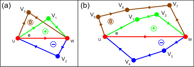
Figure 1. Sign convention for (a) directed triangles and (b) directed polygons.

We can then define the directed Ricci curvature of an edge by averaging as in differential or piecewise linear geometry as

(2.5) $$\kappa_{M}(e)\stackrel{{\scriptstyle\rm not}}{{=}}{\rm Ric}_{M}(e)=\sum_{T_{e}\sim e}\kappa_{M,O}(T_{e})\,,$$

where $T_{e}\sim e$ denote the triangles adjacent to the edge $e$; and

(2.6) $$\kappa_{M}(v)\stackrel{{\scriptstyle\rm not}}{{=}}{\rm scal}_{M}(v)=\sum_{e_{k}\sim v}{\rm Ric}_{M}(e_{k})=\sum_{T\sim v}{\kappa_{M,O}(T)}\,;$$

where, $e_{k}\sim v,T\sim v$ stand for all the edges adjacent to the vertex $v$ and all the triangles $T$ having $v$ as a vertex, respectively.

Remark 2.1.

${\rm Ric}_{M}(e)$ captures, in keeping with the intuition behind $\kappa_{M}(T)$ the geodesic dispersion rate aspect of Ricci curvature. (See [11] for a succinct overview of the different aspects of Ricci curvature.)

As already indicated, we see two drawbacks for Menger curvature as a tool in network analysis. It depends on a background geometry model, and it naturally applies only to triangles, but not to more general 2-cells. Therefore, we next turn to Haantjes curvature.

3. Haantjes curvature

Haantjes [14] defined metric curvature by comparing the ratio between the length of an arc of curve and that of the chord it subtends. More precisely, if $c$ is a curve in a metric space with metric $d$, and $p,q,r$ are points on $p$ between $q$ and $r$, the Haantjes curvature is defined as

(3.1) $$\kappa_{H}^{2}(p)=24\lim_{q,r\rightarrow p}\frac{l(\widehat{qr})-d(q,r)}{\big{(}d(q,r)\big{)}^{3}}\,\,;$$

where $l(\widehat{qr})$ denotes the length – in the intrinsic metric induced by $d$ – of the arc $\widehat{qr}$.

In the network case, $\widehat{qr}$ is replaced by a path $\pi=v_{0},v_{1},\ldots,v_{n}$, and the subtending chord by $\bar{e}=\overline{v_{0}v_{n}}$. Clearly, the limiting process has no meaning in this discrete case. Furthermore, the normalizing constant 24 which ensures that the limit will coincide, in the case of smooth planar curves, with the classical notion, is superfluous in this setting. This leads to the following definition of the Haantjes curvature of a path $\pi$:

(3.2) $$\kappa_{H}^{2}(\pi)=\frac{l(\pi)-l(v_{0}v_{n})}{l(v_{0}v_{n})^{3}}\,\,;$$

where, if the graph is a metric graph, $l(v_{0}v_{n})=d(v_{0}v_{n})$. In particular, in the case of the combinatorial metric, we obtain that, for $\pi$ as above, $\kappa_{H}(\pi)=\sqrt{n-1}$.

Clearly, one can extend the above definition to directed paths in the same manner as done for the Menger curvature, namely

(3.3) $$\kappa_{H,O}(T)=\varepsilon(\pi)\cdot\kappa_{H}(T)\,;$$

for every directed path $\pi$, where $\varepsilon\in\{-1,0,+1\}$ denotes the orientation of $\pi$.

3.1. A Local Gauss-Bonnet Theorem and the Curvature of 2-Cells

Because of its advantages over Menger curvature, we shall now use Haantjes curvature to define scalar and Ricci curvatures of networks. The basic idea here is to adapt the local Gauss-Bonnet Theorem to this discrete setting. Recall that, in the classical context of smooth surfaces, the theorem states that

(3.4) $$\iint_{D}KdA+\sum_{0}^{p}\int_{v_{i}}^{v_{i+1}}k_{g}dl+\sum_{0}^{p}\varphi_{i}=2\pi\chi(D)\,;$$

where $D\simeq\mathbb{B}^{2}$ is a (simple) region in the surface, having as boundary $\partial D$ a piecewise-smooth curve $\pi$, of vertices (i.e. points where $\partial D$ is not smooth) $v_{i},i=1,\dots,n$, ($v_{n}=v_{0}$); $\varphi_{i}$ denotes the external angles of $\partial D$ at the vertex $v_{i}$; and $K$ and $k_{g}$ denote (as usually) the Gaussian and geodesic curvatures, respectively.

We should first note that, in the absence of a background curvature, the very notion of angle is undefinable. Therefore, for abstract (non-embedded) cells, no “honest” notion of angle exists. Therefore, the last term on the left side of (3.4) above has no proper meaning, thus should be discarded. Indeed, the distances between non-adjacent vertices on the same cycle (apart from the path metric) are not defined, thus the third term in the left side of formula (3.4) vanishes.

We first concentrate on the case of combinatorial graphs. For this type of networks, i.e. endowed with the combinatorial metric, the area of each cell is commonly taken as being equal to 1. Moreover, one assumes (quite naturally) that curvature is constant on each cell. Therefore, the first term in the left side of (3.4) reduces simply to $K$. In addition, given that $D$ is a 2-cell, thus $\chi(D)=1$. It follows, that in such a setting we obtain

(3.5) $$K=2\pi-\int_{\partial D}k_{g}dl\,.$$

It is tempting to next consider $\partial D$ as being composed of segments (on which $k_{g}$ vanishes), except at the vertices, thus rendering the expression above as

(3.6) $$K=2\pi-\sum_{1}^{n}\kappa_{H}(v_{i})\,.$$

However, in general weighted graphs, one can not define a (non-trivial) Haantjes curvature for each of the vertices since, as already noted above, no proper distance between the vertices $v_{i-1}$ and $v_{i+1}$ can be implicitly assumed (apart from the one given by the path metric, which would produce trivial 0 curvature at $v_{i}$). In fact, in this general case, neither can the arc (path) $\pi=v_{0}v_{1}\ldots v_{n}$ be truly viewed as smooth. Therefore, we have no choice but to replace the right term in (3.6) above by $\kappa_{H}(\pi)$, where it should be remembered that $\pi$ represents the path $v_{0},v_{1},\ldots,v_{n}$, of chord $\bar{e}=\overline{v_{0}v_{n}}$.

We can now define the (Haantjes) sectional curvature of a 2-cell $\mathfrak{c}$. Given an edge $e=(u,v)$ and a cell $\mathfrak{c}$, $\partial\mathfrak{c}=(u=v_{0},v_{1},\ldots,v_{n}=v)$ (relative to the edge $e\in\partial\mathfrak{c}$), we put

(3.7) $$K_{H,e}(\mathfrak{c})=2\pi-\kappa_{H,e}(\pi)\,;$$

where $\pi$ denotes the path $v_{0},v_{1},\ldots,v_{n}$, subtended by the chord $\bar{e}=\overline{v_{0}v_{n}}$ (see Figure 2), and $\kappa_{H,e}(\pi)$ denotes its respective Haantjes curvature.

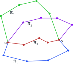
Figure 2. Haantjes-Ricci curvature in the direction $\overline{uv}$, is defined as ${\rm Ric}_{H}(\overline{uv})=\sum_{1}^{m}K^{i}_{H,\overline{uv}}=\sum_{1}^{m}\kappa_{H,\overline{uv}}(\pi_{i})$  where $\kappa_{H,\overline{uv}}(\pi_{i})=\frac{l(\pi_{i})-l(\pi_{0})}{l(\pi_{0})^{3}}\,i=1,2,3$; $\pi_{0}$ being the shortest path connecting the vertices $u$ and $v$.

Note that the definition above is much more general than the one based on Menger curvature. Indeed, not only is it applicable to cells whose boundary has (combinatorial) length greater than three (i.e. not just to triangles), it also does not presume any convexity condition for the cells, even in the case when they are realized in some model space, e.g. in $\mathbb{R}^{3}$. However, for simplicial complexes endowed with the combinatorial metric, the two notions coincide up to a constant. More precisely, in this case, for any triangle $T$, $\kappa_{M}(T)/\kappa_{H}(T)=\sqrt{3}/3$. In fact, for the case of smooth, planar curves Menger and unnormalized Haantjes curvature coincide in the limit and, furthermore, they agree with the classical concept. (However, for networks there is no proper notion of convergence, a fact which allowed us to discard the factor 24 in the original definition of Haantjes curvature.)

We can now define, in analogy with (2.6), the Haantjes-Ricci curvature of an edge $e$ as

(3.8) $${\rm Ric}_{H}(e)=\sum_{\mathfrak{c}\sim e}K_{H,e}(\mathfrak{c})=\sum_{\mathfrak{c}\sim e}(2\pi-\kappa_{H,e}(\pi))\,;$$

where the sum is taken over all the 2-cells $\mathfrak{c}$ adjacent to $e$. See Figure 3 for examples of computation of Haantjes-Ricci curvature in networks, in the directed case. See Table 1 for the comparison on a number of (undirected) standard planar and spatial grids of the various types of Ricci curvature at our disposal.

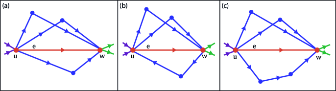
Figure 3. Haantjes-Ricci curvature ${\rm Ric}_{H}$ for directed networks, endowed with combinatorial weights: (a) ${\rm Ric}_{H}=6\pi-3$, (b) ${\rm Ric}_{H}=2\pi-1$, and (c) ${\rm Ric}_{H}=6\pi-2-\sqrt{2}$. Note that while Forman-Ricci curvature is a counter of triangles in simplicial complexes, Haantjes-Ricci curvature represents a counter of all $n$-gones, since each $n$-gone contributes a $\sqrt{n}$ term.

Curvature	Triangular	Square	Hexagonal	Euclidean
Type	Tessellation	Tessellation	Tessellation	Cubulation
${\rm Ric}_{H}(e)$	4$\pi$ - 2	4$\pi$ - 4	4$\pi-2\sqrt{2}$	8$\pi-4\sqrt{2}$
${\rm Ric}_{F,r}(e)$	-8	-2	-2	-4
${\rm Ric}_{F}(e)$	-2	0	4	4
${\rm Ric}_{O}(e)$	1	-1	–	-$\frac{4}{3}$

Table 1. Comparison of undirected curvatures for a number of standard grids (tesselations) of the Euclidean plane and space.

3.2. The case of general weights

We now return to the general case. First let us note that for general weighted graphs, it is not reasonable to attach area 1 to every 2-cell. However, as discussed in [23, 24], it is possible to endow cells in an abstract weighted network with weights that are both derived from the original ones and have a geometric content. For instance, in the case of social or biological networks, endowed with the combinatorial metric, one can designate to each face, instead of the canonical combinatorial weight equal to 1, a weight that “penalizes” the faces with more edges, thus reflecting the weaker mutual connections between the vertices of such a face. Thus, it is possible to derive a proper local Gauss-Bonnet formula for such general networks, i.e. in a manner that still retains the given data, yet captures the geometric meaning of area, volume, etc.

Thus, when considering any such geometric weight $w_{g}(\mathfrak{c}^{2})$ of a 2-cell $\mathfrak{c}^{2}$, the appropriate form of the first term on the left side of (3.4) becomes

$$Kw_{g}(\mathfrak{c}^{2})\,,$$

and the fitting form of (3.7) is

(3.9) $$K_{H,e}(\mathfrak{c})=-\frac{1}{w_{g}(\mathfrak{c}^{2})}\left(2\pi-\kappa_{H,e}(\pi)\right)\,;$$

Before passing to the problem of extending the above definition to the case of general weights, let us note that the observations above regarding Menger curvature for directed networks apply also to Haantjes curvature, after properly extending the notion of directed 1-cycles of any length and not just of directed triangles (see [24] and Figure 1). Again, as for the Menger curvature, considering directed networks actually simplifies the problem, in the sense that it allows for variable curvature (and not just a constant sign one). For general edge weights, we have the problem that the total weight $w(\pi)$ of a path $\pi=v_{0}v_{1}\ldots v_{n}$ is not necessarily smaller than the weight of its subtending chord $v_{0}v_{n}$ , thus Haantjes’ definition cannot be applied. However, we can turn this to our own advantage by reversing the roles of $w(\pi)$ and $w(v_{0}v_{n})$ in the definition of the Haantjes curvature and assigning a minus sign to the curvature of cycles for which this occurs.

Thus, this approach actually allows us to define a variable sign Haantjes curvature of cycles (hence a Ricci curvature as well), even if the given network is not a naturally directed one.

Note that the case when $w(v_{0}v_{1}\ldots v_{n})=w(v_{0}v_{n})$, i.e. that of zero curvature of the 2-cell $\mathfrak{c}$ with $\partial\mathfrak{c}=v_{0}v_{1}\ldots v_{n}v_{0}$ straightforwardly corresponds to the splitting case for the path metric induced by the weights $w(v_{i}v_{i+1})$.

Indeed, the method suggested above reduces to the use of the path metric, in most of the cases. However, both the lack of complete generality of the path metric approach and the sign assignment advantage exploited in the preceding paragraph, induced us to prefer the straightforward approach above. Of course, one can always pass to the path metric and apply to it the Haantjes curvature. Beyond the complications that this might induce in certain cases, it is, in our view, less general, at least from a theoretical viewpoint, since it necessitates the passage to a metric. However, in the case of most general weights, i.e. both vertex and edge weights, one has to pass to a metric. We find the path degree metric (see e.g. [25]) especially alluring, given that it combines simplicity with the capacity of capturing in the discrete context essential geometric properties of Riemannian metrics. (However, see also [26] for an ad hoc metric devised precisely for use on graphs in tandem with Haantjes curvature.)

3.3. A Further Generalization

Formulas (3.1) and (3.2) are meaningful not only for a single edge. We can consider any two vertices $u,v$ that can be connected by a path. Among the (simple) paths $\pi_{1},\ldots,\pi_{m}$ connecting them, the shortest one, i.e. the one for which $l(\pi_{i_{0}})=\min\{l(\pi_{1}),\ldots,l(\pi_{m})\}$ is attended represents the metric segment of ends $u$ and $v$. Therefore, given any two such vertices, we can define the Haantjes-Ricci curvature in the direction $\overline{uv}$ to be

(3.10) $${\rm Ric}_{H}(\overline{uv})=\sum_{1}^{m}K^{i}_{H,\overline{uv}}=\sum_{1}^{m}\kappa_{H,\overline{uv}}(\pi_{i})\,$$

where $K^{i}_{H,\overline{uv}}$ denotes the Haantjes-Ricci curvature of the cell $\mathfrak{c}_{i}$, where $\partial\mathfrak{c}_{i}=\pi_{i}\pi_{0}^{-1}$, relative to the direction $\overline{uv}$, and where

(3.11) $$\kappa_{H}(\pi_{i})=\frac{l(\pi_{i})-l(\pi_{0})}{l(\pi_{0})^{3}}\,,$$

and where the paths $l(\pi_{1}),\ldots,l(\pi_{m})$ satisfy the condition that $\pi_{i}\pi_{0}^{-1}$ is an elementary cycle. (This represents a locality condition in the network setting.)

We conclude this section by noting that both the directed version of curvature and the one for general weights can be extended, mutatis mutandis, to this generalized definition.

3.4. Simplified Versions for Simplicial Complexes

For networks in general, but especially in the case of simplicial complexes, it is useful to notice that Formula (3.2) for a triangle $T=T(uvw)$ reduces to

(3.12) $$\kappa^{2}_{H}(T)=\frac{d(u,v)+d(v,w)-d(u,w)}{(d(u,w))^{3}}\,.$$

Haantjes curvature of triangles is thus closely related to two other measures, namely the excess ${\rm exc}(T)$ and aspect ratio ${\rm ar}(T)$, that are defined as follows:

(3.13) $${\rm exc}(T)=\max_{v\in\{u,v,w\}}{(d(u,v)+d(v,w)-d(u,w))}\,;$$

(3.14) $${\rm ar}(T)=\frac{e(T)}{d(T)}\,;$$

where $d(T)$ denotes the diameter of a triangle $T=T(uvw)$.

There are strong connections between the excess, aspect ratio, and curvature. In particular, for the normalized Haantjes curvature introduced above, we have the following relation between the three notions:

(3.15) $$\kappa_{H}^{2}(T(v))=\frac{e(T(v))}{d^{3}}\,,$$

that is

(3.16) $$\kappa_{H}(T(v))=\frac{\sqrt{{\rm ar}(T(v))}}{d}\,.$$

Since the factor $\frac{1}{d}$ has the role of ensuring that, in the limit, the curvature of a triangle will have the dimensionality of the curvature at a point of a planar curve, the aspect ratio can be viewed as a (skewed), un-normalized version of curvature (and Haantjes curvature can be viewed as a scaled version of excess). Thus, since the notion of scale is not of true import in many aspects of network understanding, curvature can be replaced by these surrogates.

Also, for the global understanding of the shape of networks, it is useful to compute, as is common in the manifold context, the maximal excess and minimal aspect ratio over all triangles in the network.

4. Conclusions and Further Work

In the present paper we have shown that, based on two classical notions of metric curvature, namely the Menger and Haantjes curvatures, it is easy to define expressive notions of curvature, for networks and their higher-dimensional generalizations, as well as for simplicial and clique complexes. In particular, it is possible to define metric Ricci curvatures for quite general networks – both with vertex and edge weights. Furthermore, due to the simple definitions of the metric curvatures residing at the base of these definition, the new definitions are computationally efficient (especially those based on Menger curvature), while being, at the same time, extremely versatile (in particular those derived from Haantjes curvature). In fact, for combinatorial polyhedral complexes, it proves to be more expressive than the (full) Forman curvature, since it takes general $n$-gones into account, and not just of triangles.

The metric definition based on the so called Wald metric curvature proposed in [17] allows for the easy derivation of convergence results as well as the proof of theoretical results, such as a polyhedral version of the classical Bonnet-Myers Theorem, but it is computationally extremely expensive, rendering it practically prohibitive as far as concrete calculations are concerned. This is in stark contrast with the simplicity and efficiency of the methods developed in the present article.

Since the permitted length of this article is limited, we could only introduce the main ideas and definitions, and could treat neither possible applications, nor deeper theoretical aspects. Concerning the implementation aspect is concerned, we see two immediate and necessary tasks that we hope to develop further. The first one is a statistically significant comparison of the various extant notions of Ricci curvature – Forman, reduced Forman, Ollivier, Stone, etc. on large empirical and model networks. The second one is the exploration of the clustering and community detection capabilities of the Ricci curvature notions introduce herein, and their comparison, with the results in [26] and [5, 27] respectively. Furthermore, it would be interesting to explore the correlation between the notions of curvature introduced herein and hyperbolic embeddings of networks. In particular, one would like to explore to what extent the curvatures predict values using the inferred hyperbolic distances among nodes (points) in embeddings like the one considered in [28], and see how much these values agree with or deviate from the curvatures measured on the observed network. On the theoretical end of the spectrum, one would naturally like to prove analogues of such results as the Bonnet-Myers Theorem already mentioned above and, most importantly, of a fitting analogue of the fundamental global Gauss-Bonnet Theorem, with important applications in the study of long time evolution of networks [29].

References

- [1] Eckmann, J.-P., Moses, E.: Curvature of co-links uncovers hidden thematic layers in the World Wide Web. PNAS 99 (2002) 175–181.
- [2] Ollivier, Y.: Ricci curvature of Markov chains on metric spaces. Journal of Functional Analysis, 256(3) (2009) 81–864.
- [3] Ni, C.-C., Lin, Y.-Y., Gao, J., Gu, X.D., Saucan, E.: Ricci Curvature of the Internet Topology. In: Proceedings of INFOCOM 2015, pp. 2758–2766, IEEE (2015).
- [4] Sandhu, R., Georgiou, T., Reznik, E., Zhu, L., Kolesov, I., Senbabaoglu Y., Tannenbaum, A.: Graph curvature for differentiating cancer networks. Scientific Reports, 5 (2015) 12323.
- [5] Ni, C.-C., Lin, Y.-Y., Luo, F.,Gao, J.: Community Detection on Networks with Ricci Flow. Scientific reports, 9(1) (2019) 9984.
- [6] Simhal, A.K., Carpenter, K.L.H., Nadeem, S., Kurtzberg, J., Song, A., Tannenbaum, A., Sapiro, G., Dawson, G.,: Measuring Robustness of Brain Networks in Autism Spectrum Disorder with Ricci Curvature, bioRxiv, (2018) 722025.
- [7] Asoodeh, S., Gao, T., Evans, J.: Curvature of Hypergraphs via Multi-Marginal Optimal Transport. In: 2018 IEEE Conference on Decision and Control (CDC), pp. 1180–1185. IEEE, (2018).
- [8] Sreejith, R.P., Mohanraj, K., Jost, J., Saucan, E., Samal, A.: Forman curvature for complex networks. Journal of Statistical Mechanics: Theory and Experiment, (2016) 063206.
- [9] Weber, M., Saucan E., Jost, J.: Characterizing Complex Networks with Forman-Ricci curvature and associated geometric flows. J. Complex Netw., 5(4) (2017) 527–550.
- [10] Forman, R.: Bochner’s Method for Cell Complexes and Combinatorial Ricci Curvature. Discrete and Computational Geometry, 29(3) (2003) 323–374.
- [11] Samal, A., Sreejith, R.P., Gu, J., Liu, S., Saucan, E., Jost, J.: Comparative analysis of two discretizations of Ricci curvature for complex networks. Scientific Reports, 8(1) (2018) 8650.
- [12] Jost, J.: Riemannian Geometry and Geometric Analysis. Springer Verlag, Berlin (2011)
- [13] Menger, K.: Zur Metrik der Kurven. Matematische Annalen, 103 (1930) 466–501.
- [14] Haantjes, J.: Distance geometry. Curvature in abstract metric spaces. Proc. Kon. Ned. Akad. v. Wetenseh., Amsterdam 50 (1947) 496–508.
- [15] Saucan, E.: Metric Curvatures and their Applications I. Geometry, Imaging and Computing, 2(4) (2015) 257–334.
- [16] Saucan, E.: Metric Curvatures and their Applications 2: Metric Ricci Curvature and Flow. arXiv:1902.03438.pdf, 1-39 (2018).
- [17] Gu, D.X., Saucan, E.: Metric Ricci curvature for manifolds. Geometry, (2013) 694169.
- [18] Bianconi, G., Rahmede, C.: Emergent hyperbolic network geometry. Scientific Reports, 7 (2017) 41974.
- [19] Krioukov,D., Papadopoulos,F., Kitsak,M., Vahdat, A., Boguna, M.: Hyperbolic Geometry of Complex Networks. Phys. Rev. E 82 (2010) 036106.
- [20] Zeng, W., Sarkar, R., Luo, F., Gu, X., Gao, J.: Resilient routing for sensor networks using hyperbolic embedding of universal covering space. In: INFOCOM 2010, pp. 1–9. IEEE (2010).
- [21] Janson, S.: Euclidean, spherical and hyperbolic trigonometry. Lecture notes (2015), 1–53, http://www2.math.uu.se/ svante/papers/sjN16.pdf.
- [22] Saucan, E., Sreejith, R.P., Vivek-Ananth, R.P., Jost, J., A. Samal. Discrete Ricci curvatures for directed networks. Chaos, Solitons & Fractals, 118 (2019) 347-360.
- [23] Horak D., J.Jost, J.: Spectra of combinatorial Laplace operators on simplicial complexes. Advances in Mathematics, 244 (2013) 303–336.
- [24] Saucan, E., Weber, M.: Forman’s Ricci curvature - From networks to hypernetworks. In: Proceedings of COMPLEX NETWORKS VII, Studies in Computational Intelligence (SCI) vol. 812, pp. 706–717. Springer, Berlin (2019).
- [25] Keller, M.: Intrinsic Metrics on Graphs: A Survey, In: Mugnolo, D. (eds) Mathematical Technology of Networks. Springer Proceedings in Mathematics & Statistics, 128, Springer, Cham (2015).
- [26] Saucan, E., Appleboim, E.: Curvature Based Clustering for DNA Microarray Data Analysis. In: Iberian Conference on Pattern Recognition and Image Analysis 2005. LNCS, vol. 3523, 405-412, Springer, Berlin 2005.
- [27] Sia, J., Jonckheere, E., and Bogdan, P. Ollivier-Ricci Curvature-Based Method to Community Detection in Complex Networks. Scientific Reports, 9(1) (2019) 9800.
- [28] Boguná, M., Papadopoulos, F., Krioukov, D..: Sustaining the internet with hyperbolic mapping. Nature communications, 1 (2010) 62.
- [29] Weber, M., Saucan, E., Jost, J.: Coarse geometry of evolving networks. J. Complex Netw., 6(5) (2018) 706–732.