Aeolian dune modelling from airborne LiDAR, terrestrial LiDAR and Structure from Motion–Multi View Stereo

Abstract

Sand dunes are commonly regarded as a challenge to traditional photogrammetry due their homogeneous texture and spectral response. In this work we present an evaluation of Structure from Motion–Multi View Stereo (SfM-MVS) to obtain high-resolution elevation data of coastal sand dunes based on images acquired by Remotely Piloted Aircraft (RPA). A Digital Elevation Model (DEM) of a dunefield in Southern Brazil was generated from 810 photos captured by an RPA at 100 m above the takeoff point in February 2019. Image matching was successful in all areas of the survey due the presence of superficial features (footprints and sandboard tracks) and visibility of the sedimentary stratification, highlighted by heavy minerals. Altimetric accuracy of the SfM-MVS DEM was validated by comparison with Terrestrial LiDAR (TLS) data collected during the same fieldwork campaign of the RPA flights. The SfM-MVS DEM was then compared to an Airborne LiDAR (ALS) DEM from October 2010. While the SfM-MVS and TLS DEMs are very similar, without any major difference in elevation or in the reconstruction of topographic features, the SfM-MVS DEM presents a small scale surface roughness not visible in the TLS DEM. The Feature Preserving DEM Smoothing (FPD) algorithm was applied to the SfM-MVS DEM with good results in terms of surface smoothing, but without any significant changes in descriptive statistics and error metrics, with an RMSE of 0.08 m and MAE of 0.06 m for both the original and the FPD-filtered DEM.

Displacement of dune crest lines from the ALS and SfM-MVS DEMs resulted in a migration rate of $\approx$5 m/year between 2010 and 2019, in good agreement with rates derived from satellite images and historical aerial photographs of the same area. Sand volume change in the same period showed a decrease of only 0.2%, which can be related to the installation of sand fences to promote dune stabilization and sand removal from the front of the dune field to keep a road open to vehicles. ALS can cover large areas in little time but its high cost still remains a barrier to wider usage, especially by researchers in developing countries. TLS has an intermediate cost but demands more fieldwork and more processing time. In our case we needed three days for the TLS survey and around three weeks to produce a DEM of $\approx$$80\text{~{}}400$$\mathrm{m}^{2}$. On the other hand, we were able to cover $\approx$$740\text{~{}}900$$\mathrm{m}^{2}$ with six flight missions in under three hours, with $\approx$13 hours processing time in a medium-range workstation. This makes SfM-MVS a low-cost solution with fast and reliable results for 3D modelling and continuous monitoring of coastal dunes.

Cite as: Grohmann, C.H., Garcia, G.P.B., Affonso, A.A., Albuquerque, R.W., 2020. Aeolian dune modelling from airborne LiDAR, terrestrial LiDAR and Structure from Motion–Multi View Stereo. Computers & Geosciences. 143:104569. doi:10.1016/j.cageo.2020.104569

url]http://www.iee.usp.br, https://spamlab.github.io

1 Introduction

Aeolian dune fields occur in diverse depositional settings, on Earth and on other planetary bodies such as Mars, Venus, Saturn’s moon Titan and Pluto (Fryberger and Dean, 1979; Short, 1988; Wang et al., 2002; Livingstone et al., 2007; Hayward et al., 2007; Radebaugh et al., 2008; Bourke et al., 2010; Martinho et al., 2010; Kreslavsly and Bondarenko, 2017; Hayes, 2018; Telfer et al., 2018). To better understand these dynamic environments, repeated topographic surveys of the landscape are needed (Conlin et al., 2018). As the sand supply of dune fields is sensitive to patterns of wind and rainfall, changes in dune field volume and morphology can be related to climate change (Gaylord et al., 2001; Clemmensen et al., 2007; Sawakuchi et al., 2008; Tsoar et al., 2009; Singhvi et al., 2010; Levin, 2011; Grohmann and Sawakuchi, 2013; Hoover et al., 2018).

Migration rates of aeolian dunes have been determined with aerial photographs (e.g., Finkel, 1961), orbital imagery (Shrestha et al., 2005; Potts et al., 2008; Hugenholtz and Barchyn, 2010; Dong, 2015; Mendes and Giannini, 2015; Mendes et al., 2015; Bhadra et al., 2019) or Digital Elevation Models (DEMs) (e.g., Mitasova et al., 2005b).

With the growth of Geomorphometry as the practice of terrain modelling and ground-surface quantification (Pike, 1995; Pike et al., 2009; Hengl and Reuter, 2008), DEMs have became essential tools in landform analysis, as they allow speed, precision and reproducibility to calculation of geomorphometric parameters (Grohmann, 2004).

DEMs of aeolian dunes can be constructed by several methods such as traditional field techniques (levelling, Total Station) (Łabuz, 2016), interpolation of contour lines (Judge et al., 2000; Mitasova et al., 2005b), Differential or Real-time kinematic (RTK) GPS points (Mitasova et al., 2005b; Pardo-Pascual et al., 2005), LiDAR (Light Detection and Ranging) surveys, either airborne (ALS - Airborne Laser Scanner) (Mitasova et al., 2004, 2005a, 2005b; Vianna and Calliari, 2015; Baughman et al., 2018), terrestrial (TLS - Terrestrial Laser Scanner) (Montreuil et al., 2013; Feagin et al., 2014; Fabbri et al., 2017; Sankey et al., 2018b; Bañón et al., 2019; Kasprak et al., 2019; Lee et al., 2019) or mounted on Remotely Piloted Aircrafts (RPAs) (Solazzo et al., 2018; Garcin et al., 2019), and Structure from Motion–Multi View Stereo (SfM-MVS) using images collected by handheld cameras, mounted on poles, kites or RPAs (Mancini et al., 2013; Gonçalves and Henriques, 2015; Conlin et al., 2018; Duffy et al., 2018; Forlani et al., 2018; Seymour et al., 2018; Solazzo et al., 2018; Guisado-Pintado et al., 2019; Laporte-Fauret et al., 2019; Kasprak et al., 2019; Lee et al., 2019; O’Dea et al., 2019; Pagán et al., 2019; Taddia et al., 2019). A literature review on RPA-based topographic surveys of coastal areas is presented by Casella et al. (2020).

In this work we present an evaluation of SfM-MVS to obtain high-resolution elevation data of coastal sand dunes. Altimetric accuracy of the SfM-MVS DEM was validated by comparison with TLS data collected during the same fieldwork campaign of the RPA flights (February 2019). The SfM-MVS DEM was then compared to an ALS DEM from October 2010. The results show almost no change in total volume and a migration rate of $\approx$5 m/year, compatible with those derived from aerial and orbital imagery.

While 3D modelling of aeolian sand dunes can be a challenge to traditional photogrammetry due to their homogeneous texture and spectral response, the use of SfM-MVS is recommended and the factors that contributed to a successful reconstruction are discussed.

1.1 Study area

The study area, located in Santa Catarina State, southern Brazil (Fig. 1A-B), comprises barrier-lagoon depositional systems with associated dune fields (Angulo et al., 2006; Giannini et al., 2007) which evolved during the Late Holocene as a result of wind strength intensification and sand supply increase in southern Brazilian coast (Mendes and Giannini, 2015; Mendes et al., 2015). The Garopaba (or Siriú) dune field is composed of unvegetated and vegetated aeolian dunes. The unvegetated dunes are represented by mostly barchanoid chains, while the vegetated ones include parabolic dunes, blowouts and foredunes (Martinho et al., 2006; Hesp et al., 2007).

There are significant differences of wind field along the southern Brazilian coast; while the dominant and prevailing direction is from the S at Joaquina (located $\approx$$45$$\mathrm{k}\mathrm{m}$ north of Garopaba in Santa Catarina Island), it is from the NE at Farol de Santa Marta, $\approx$$70$$\mathrm{k}\mathrm{m}$ south of the study area (Dillenburg et al., 2006; Hesp et al., 2007; Truccolo, 2011; Mendes and Giannini, 2015). At Garopaba, winds from the North are responsible for dune migration (Mendes and Giannini, 2015; Mendes et al., 2015).

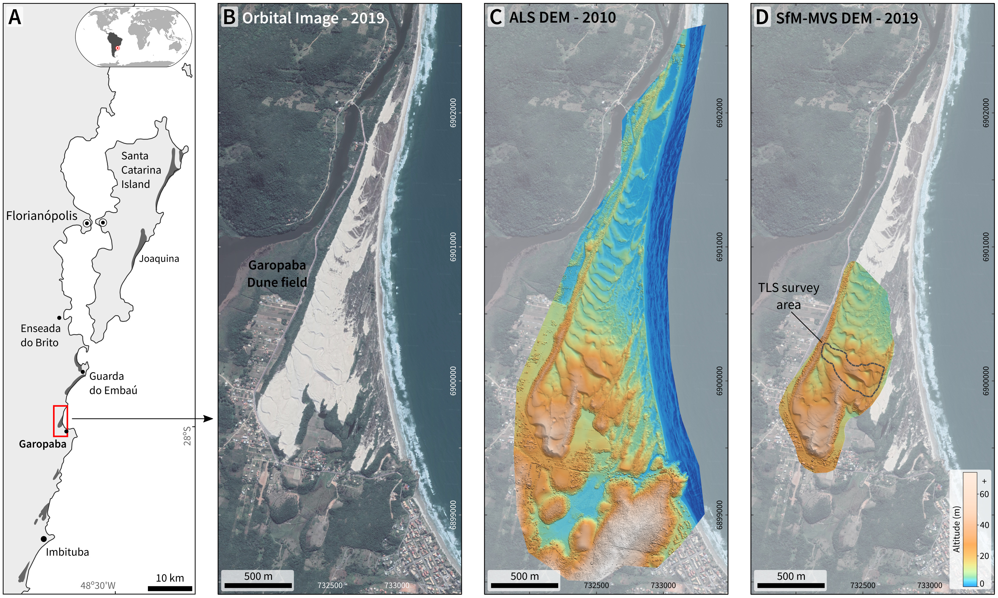
Figure 1: A) Location of study area in southern Brazil; B) Satellite image of the Garopaba dune field (image date: 07-30-2017); C) Digital Surface Model produced by ALS (2010); D) DEM produced by SfM-MVS (2019), with TLS survey area shown. Elevation colour scale is the same for C and D. Shaded relief illumination: N$025\mathrm{°}$, $30\mathrm{°}$ above horizon. Dune field satellite imagery ©2019 Maxar Technologies, powered by Google. Coordinate system for B/C/D and following figures: UTM zone 22 southern hemisphere, WGS84 datum.

2 Methods

This section presents the datasets, methods and tools used in this study. A flowchart of the analysis steps is in the Supplemental Material. Table 1 shows, for each kind of data used in this paper (ALS, SfM-MVS, TLS), area of the interpolated DEM, number of points and density of points within that area.

Table 1: Overview of datasets used in this study. See text for details and Supplemental Material for maps of point density.

Data	DEM Area ($\mathrm{m}^{2}$)	# points	points/$\mathrm{m}^{2}$
ALS (full)	$4\text{~{}}434\text{~{}}722$	$11\text{~{}}574\text{~{}}555$	$2.6$
ALS (SfM area, 1st returns)	$740\text{~{}}922$	$2\text{~{}}380\text{~{}}005$	$3.2$
SfM-MVS (full)	$740\text{~{}}922$	$344\text{~{}}769\text{~{}}434$	$465.3$
SfM-MVS (thin 125th pt)	$740\text{~{}}922$	$2\text{~{}}378\text{~{}}399$	$3.2$
SfM-MVS (TLS area)	$80\text{~{}}413$	$28\text{~{}}158\text{~{}}102$	$350.1$
SfM-MVS (10 cm grid)	$80\text{~{}}413$	$8\text{~{}}079\text{~{}}569$	$100.5$
TLS (full)	$80\text{~{}}413$	$1\text{~{}}187\text{~{}}708\text{~{}}492$	$14\text{~{}}770.1$
TLS (2 cm filter)	$80\text{~{}}413$	$170\text{~{}}141\text{~{}}709$	$2\text{~{}}115.8$
TLS (10 cm grid)	$80\text{~{}}413$	$7\text{~{}}039\text{~{}}501$	$87.5$

2.1 Airborne LiDAR

Airborne LiDAR (ALS) data were collected on October 2010 by Geoid Laser Mapping Co. using an Optech ALTM 3100 sensor with a saw-tooth scanning pattern, density of about one point per 0.5 m², measured from an altitude of $\approx$$1\text{~{}}200$ m ($\approx$$4\text{~{}}000$ ft). Raw LiDAR data (with up to four laser pulses) were processed by Geoid and delivered with vertical accuracy of 0.15 m ($1\sigma$) and horizontal accuracy of 0.5 m ($1\sigma$).

ALS data (LiDAR 1^st returns) were imported into GRASS-GIS (Neteler et al., 2012) as vector points and interpolated with bilinear splines (Brovelli and Cannata, 2004; Brovelli et al., 2004) to create a DEM with 0.5 m spatial resolution (Fig. 1C).

2.2 Fieldwork and Ground Control Points

Fieldwork for TLS and SfM-MVS surveys was conducted on February 2019. Six targets were deployed within the dune field area (Fig. 2B) and their coordinates were determined by Differential Global Positioning System (DGPS), to serve as Ground Control Points (GCPs) for georeferencing the SfM-MVS outputs and the TLS point cloud (Harwin et al., 2015).

Each target measured $\approx$80x60 cm in a black and white chequered pattern and was clearly visible in the photos (Fig. 2C). A Spectra Precision SP60 DGPS was used in a base-rover static configuration and raw data was post-processed in Survey Office 4.10 software, using the Imbituba Station of the Brazilian GPS Network as reference. The processing reports are available in the Supplemental Material.

Figure 2: A) Flight missions executed over the dune field; B) Ground Control Points used to georeference the SfM-MVS outputs and TLS data; C) Target (GCP 01), sedimentary structures and superficial features seen in the RPA photo.

2.3 Terrestrial LiDAR

Terrestrial LiDAR (TLS) data were collected with a FARO™ Laser Scanner Focus^3D S120, a geodetic laser scanner with distance measurement based on phase shift of infrared light (905 nm), maximum range of 120 m, and ranging error of $\pm$2 mm at 10 m distance at 90% reflectivity (FARO Technologies Inc., 2013). The scanner was set at resolution of “1/5” and quality of “3x”, resulting in a point spacing of 7.67 mm at a distance of 10 m, scan time of two minutes and 28.4 million points per scan (this model does not acquire images). Five spherical targets provided with the equipment were arranged on the ground at $\approx$10 m from the TLS and re-positioned in a ‘leapfrog’ scheme during the survey, so that each consecutive scan was able to capture at least two spheres from the previous one. In three days of field work, 110 scans were collected, covering an area of $\approx$$80\text{~{}}400$ m² (Fig. 1D).

TLS data were processed in FARO Scene 7.1. Each scan was registered to its adjacent ones manually using the spherical targets as references. Georreferencing of the point cloud was based on two DGPS points located at the extremities of the surveyed area (Fig. 2B). Referencing with only two points was possible because this TLS model has an integrated dual axis compensator to automatically level the captured scan data, so the control points were used for an affine transformation (translation/scale/rotation) in 2D space.

To overcome the heterogeneous distribution of data common to terrestrial LiDAR, with a very high density of points near the scanner, the full point cloud was subsampled in FARO Scene with a minimum distance filter of 2 cm between points. To eliminate duplicate points and compensate for small differences in the alignment of individual scans, this point cloud was gridded to a raster in GRASS-GIS using the mean elevation value of LiDAR points within 10 cm cells (r.in.xyz module). To fill empty (null) cells, the raster was converted to vector and a DEM with 10 cm spatial resolution was created by interpolation with bilinear splines (Fig. 4A).

2.4 SfM-MVS

Images for the SfM-MVS reconstruction were acquired by a DJI Phantom 4 Pro RPA. The aircraft digital camera has an 1” CMOS 20MP sensor, global shutter, $84\mathrm{°}$ FOV and 8.8 mm focal distance (24 mm at 35 mm equivalent). Images can be saved as JPEG or RAW, $5\text{~{}}472$$\times$$3\text{~{}}648$ px (3:2 ratio). Flight missions were planned and executed using the MapPilot app with height above takeoff point of 100 m (image footprint 150$\times$100 m, pixel size $\approx$2.7 cm) and 75% overlap along and across-track.

Six missions were flown, covering an area of $\approx$$869\text{~{}}000$ m² with 810 images. The camera angle was set to $-80\mathrm{°}$ (i.e., $10\mathrm{°}$ from nadir). Figure 2A shows flight paths and starting time for each mission (UTC-3). Weather conditions during fieldwork were of dark skies with light rains scattered throughout the day.

The SfM-MVS workflow (e.g., Westoby et al., 2012; Viana et al., 2018; James et al., 2019) was processed in Agisoft Metashape Pro version 1.5.1. In the SfM step, images were aligned with ‘High’ accuracy. To avoid doming effects in the reconstructed surface (e.g., James and Robson, 2014), camera alignment optimization was performed considering a marker accuracy of 0.005 m, following Agisoft’s recommendations. The MVS reconstruction was set to ‘High’ quality and ‘aggressive’ depth filtering. The processing report is available in the Supplemental Material.

For the altimetric comparison with TLS data, the full SfM-MVS point cloud was imported into GRASS-GIS in the same manner of the TLS data: gridded by the mean elevation in 10 cm cells, converted to vector and interpolated with bilinear splines to a DEM with 10 cm resolution (Fig. 4B).

For the dune migration and volume analysis, the full SfM-MVS point cloud was subsampled (thinned) with LAStools (Isenburg, 2019) by extracting every 125^th point, imported into GRASS-GIS as vector points and interpolated with bilinear splines to a DEM with 0.5 m resolution (Fig. 1D). The thinning value was determined after experimentation, and the goal was to obtain a similar number of points, within the interpolation area, for the ALS and SfM point clouds (Table 1).

2.4.1 Accuracy of SfM-MVS DEM

The vertical accuracy of a DEM can be computed from the differences between the dataset being analyzed and co-located values from an independent source of higher accuracy (Willmott and Matsuura, 2005; Wechsler, 2007; Hebeler and Purves, 2009; Reuter et al., 2009; Baade and Schmullius, 2016). To evaluate the accuracy of the SfM-MVS reconstruction, the TLS DEM was considered as the reference.

Mean Absolute Error (MAE) and Root Mean Square Error (RMSE) are metrics that been widely used in the Geosciences to measure the accuracy of DEMs (e.g., Nikolakopoulos et al., 2006; Willmott and Matsuura, 2006; Smith and Vericat, 2015; Gesch et al., 2016; Satge et al., 2016; Grohmann and Sawakuchi, 2013; Grohmann, 2018). MAE (Eq. 1) and RMSE (Eq. 2) were calculated from all pixels within a mask designed to avoid areas with vegetation or without TLS data.

$$MAE=\dfrac{1}{n}\textstyle\sum_{i=1}^{i=n}(|z_{TLS}-z_{SfM}|)$$ (1)

$$RMSE=\sqrt{\dfrac{1}{n}\textstyle\sum_{i=1}^{i=n}\Big{[}(z_{TLS}-z_{SfM})^{2}\Big{]}}$$ (2)

2.4.2 Surface roughness and DEM smoothing

Surface roughness characterizes elevation variations over a particular scale (Grohmann et al., 2010; Berti et al., 2013; Grohmann and Hargitai, 2014; Smith, 2014). In this paper surface roughness was calculated as the standard deviation of slope in a moving-window filter, as it provide good results in identifying terrain features and is not sensitive to spurious data (Grohmann et al., 2010).

Low-pass filters are usually applied to DEMs to remove or reduce roughness (Reuter et al., 2009; Gallant, 2011; Lindsay et al., 2019), but sharp edges such as dune crests will be modified as well (Barash, 2002; Grohmann and Riccomini, 2009). To retain the sharpness of breaks-of-slope in the filtered DEM edge-preserving (or de-noise) procedures (e.g., Sun et al., 2007; Stevenson et al., 2010; Lindsay et al., 2019) must be employed.

The effect of de-noising the SfM-MVS DEM was evaluated by applying the Feature Preserving DEM Smoothing (FPD) algorithm (Lindsay et al., 2019), with different parameter settings, to a sub-area of the DEM (Fig. 5) and evaluating the change of RMSE from the TLS DEM and of Circular Variance of Aspect (CVA – Lindsay et al., 2019) for each set of parameters. CVA measures the variability of aspect, or surface shape complexity, within a neighborhood; its value is 0.0 in smooth areas approaching 1.0 in areas of complex topography (i.e., high surface roughness). The three parameters to be set in the FPD method are the filter kernel size ($k$), the normal difference threshold angle ($t$), and the number of elevation-update iterations ($i$) (for a detailed explanation of the algorithm and parameters’ definitions, see Lindsay et al., 2019).

The tests were done by changing one parameter while keeping the other two fixed, and then calculating CVA for each DEM with filter sizes of $3\times 3$ up to $41\times 41$ pixels.

In the first experiment, $t$ ranged from $5\mathrm{°}$ to $45\mathrm{°}$ (in $5\mathrm{°}$ increments) with $k=15$ and $i=5$. Next, $k$ changed from $5\times 5$ up to $51\times 51$ with $t=$$$ and $i=5$. Last, $i$ varied between 3 and 30 iterations whith $k=15$ and $t=$$$.

After the sub-area tests, $k$, $t$ and $i$ values were selected and FPD was applied to the entire SfM-MVS DEM. Error metrics (RMSE, MAE) of the original and smoothed SfM-MVS DEM were calculated considering the TLS DEM as reference.

2.5 Dune Migration and Sand volume

Dune migration can be evaluated from multi-temporal data such as aerial photographs (Finkel, 1961; Stafford and Langfelder, 1971; Mendes and Giannini, 2015; Baughman et al., 2018), satellite images (Hoover et al., 2018; Dong, 2015; Yang et al., 2019) or LiDAR DEMs (Mitasova et al., 2004, 2005a, 2005b; Baughman et al., 2018). Dune migration between the 2010 (ALS) and 2019 (SfM-MVS) surveys was determined as the displacement of dune crest lines.

For each survey, surface roughness of the DEM was calculated as the standard deviation of slope (Grohmann et al., 2010) in a 5x5 pixels neighbourhood (2.5$\times$2.5 m); crest lines were drawnn in QGIS version 3.8 (QGIS Development Team, 2019) following the high-roughness crests (see Supplemental Material); lines connecting the crests were draw approximately parallel to the S-SW migration direction (Hesp et al., 2007; Mendes and Giannini, 2015) (Fig. 3) and saved in shapefile format. Azimuth and length of each displacement line were calculated with Python version 3.7.4 (Python Software Foundation, 2019) using the ogr module of the GDAL library (GDAL Development Team, 2019) to access vector geometries. Mean azimuth was calculated according to Fisher (1993).

Sand volume was calculated with the GRASS-GIS r.volume module (Hinthorne, 1988). This module calculates volume by summing cell values within a given area and then multiplying by the area occupied by those cells. An elevation of 0 m (zero) was used as a reference base level.

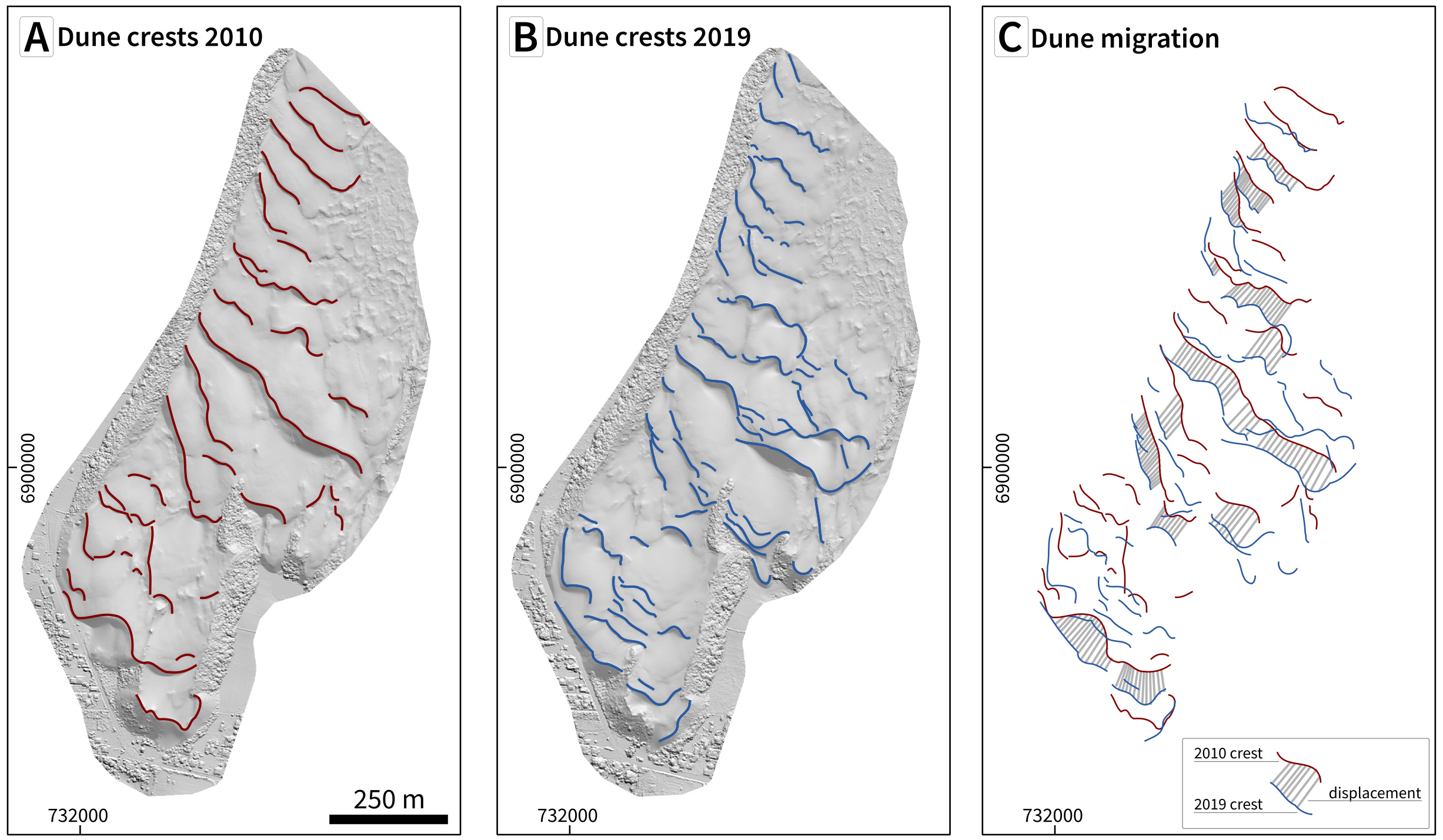
Figure 3: Determination of dune migration between 2010 and 2019 surveys. A) dune crests of 2010, over shaded relief image of ALS DEM; B) dune crests of 2019, over shaded relief image of SfM-MVS DEM; C) displacement lines (grey) connecting crest lines.

2.6 Data Analysis

In order to streamline the process and ensure reproducibility (Barnes, 2010), data analysis was performed in GRASS-GIS version 7.6 (Neteler et al., 2012; GRASS Development Team, 2019) through Jupyter notebooks (Kluyver et al., 2016; Rule et al., 2018) using the Pygrass library (Zambelli et al., 2013) to access GRASS’ datasets. The FPD algorithm is implemented in the open-source geospatial analysis platform WhiteboxTools (Lindsay, 2017). Statistical analyses were performed with the Python libraries Rasterio, Scipy, Numpy, Pandas, Seaborn and Matplotlib (Oliphant, 2006; Hunter, 2007; McKinney, 2011; Gillies et al., 2013–; The SciPy community, 2013; Waskom et al., 2016).

3 Results

3.1 TLS and SfM-MVS

The SfM-MVS survey resulted in data with 2.77 cm resolution (1.1 px reprojection error) and RMSE of 0.7 cm in longitude and 0.4 cm in latitude, and 0.5 cm in elevation for the residuals of control points (see Supplemental Material). The TLS point clouds were combined into a single dataset with a registration error of 4.9 mm.

The DEMs produced from the TLS and SfM-MVS data are presented in Fig. 4. The surfaces are very similar, without any major difference in elevation or in the reconstruction of topographic features. Upon a closer inspection, the SfM-MVS DEM presents a small scale surface roughness not visible in the TLS DEM. To visually evaluate this difference, surface roughness of the DEMs was calculated as the standard deviation of slope in a 5x5 pixels neighbourhood (0.5$\times$0.5 m).

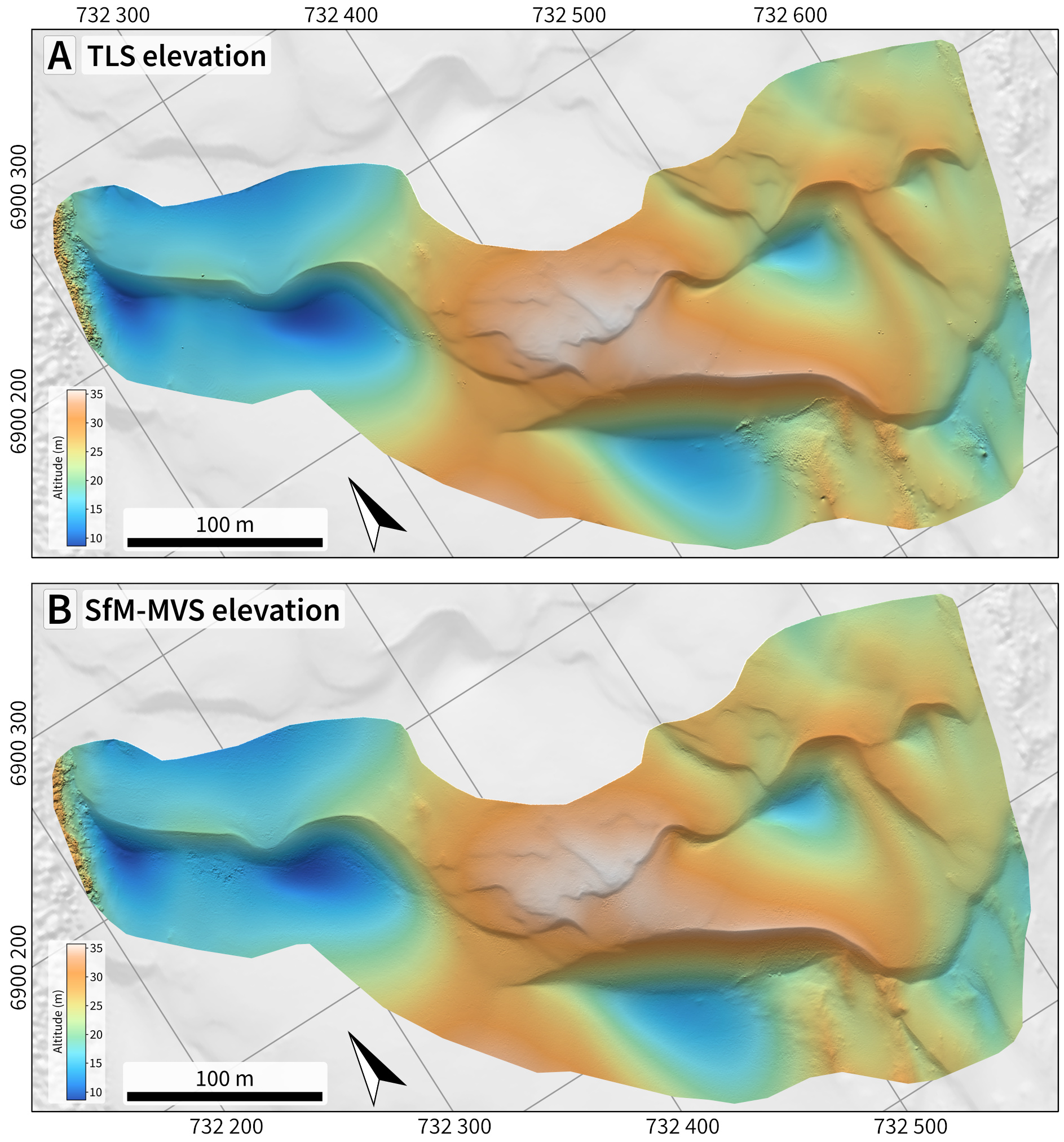
Figure 4: A) TLS DEM; B) SfM-MVS DEM. Elevation colour scale is the same for A and B. Shaded relief illumination: N$025\mathrm{°}$, $30\mathrm{°}$ above horizon.

The TLS DEM has a smooth surface, with higher roughness values on vegetated areas and over some of the places where the TLS equipment was positioned (Fig. 5A). These spots can be related to a small mismatch between adjacent scans, where in one there is no data (under the scanner), so the gridding procedure cannot compensate the difference and the result is a small circular patch of the terrain slightly above or below its surroundings. Dune crests are well marked by above-average roughness. Footprints and track marks are also visible, with lower roughness values.

The SfM-MVS DEM shows a widespread distribution of low and average roughness values (Fig. 5B). While the dune crests can be identified, track marks are no longer visible and the patch of vegetation near the sandboard tracks cannot be discriminated based on its roughness. A set of footprints seen in the central-eastern portion of the TLS roughness map is not visible in the SfM-MVS roughness because the SfM-MVS survey was carried out before the TLS survey could cover that area. We see this roughness as a noise inherent to the SfM process due to small errors in geolocation as well as to the consumer-grade quality of the photographic camera (Mosbrucker et al., 2016).

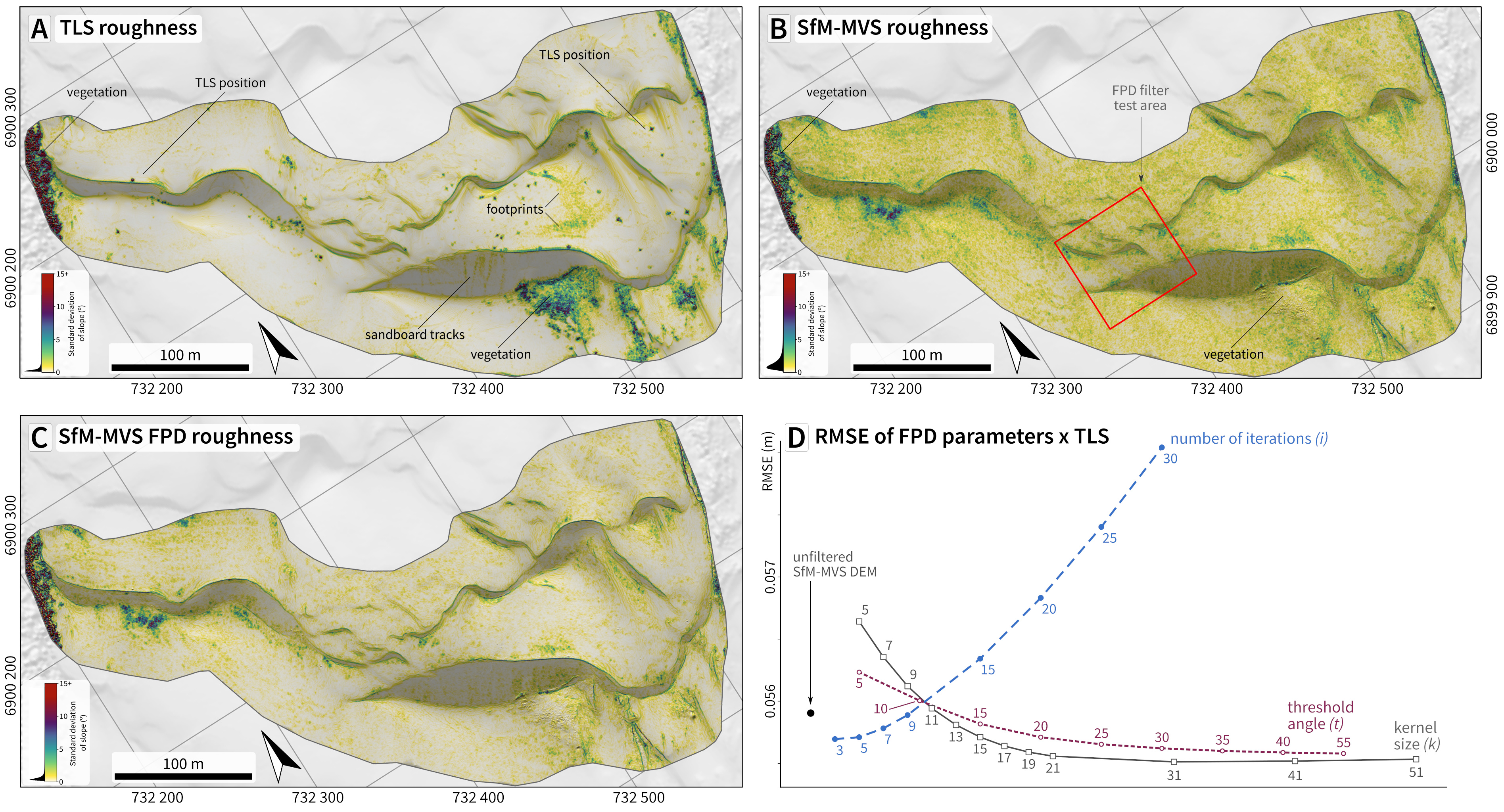
Figure 5: Surface roughness maps, calculated as the standard deviation of slope in a 5x5 window: A) TLS; B) SfM-MVS; C) SfM-MVS after FPD filter ($k=17$, $t=$$$, $i=5$); D) RMSE plot of each FPD DEM with TLS DEM according to FPD parameters. Roughness colour scale is the same for A, B and C.

Applying the FPD algorithm to a sub-area of the SfM-MVS DEM shows the RMSE between the smoothed DEM and the TLS DEM decreasing with larger FPD kernel sizes and higher angular treshold values, but increasing with the number of interactions (Fig. 5C). Considering these results, we applied FPD to the SfM-MVS DEM with $k=17\times 17$ $t=$$$ and $i=5$ (Fig. 5D). An evaluation of Circular Variance of Aspect for each parameter leads to similar conclusions, and is presented in the Supplemental Material.

The vertical accuracy of the SfM-MVS DEM, calculated for all pixels within the mask shown in Fig. 6A resulted in RMSE of 0.08 m and MAE of 0.06 m for both the original and the FPD-filtered DEM.

Descriptive statistics of the TLS and SfM-MVS DEMs are very similar (Table 2). Considering all pixels of the DEMs, elevation differences range from -1.5 m to +0.5 m, with mean of 0.0 m and standard deviation of 0.08 m; with a random sample of $2\text{~{}}000$ pixels, elevation differences range from -0.3 m to +0.5 m, with mean of 0.0 m and standard deviation of 0.08 m, The negative differences below -0.5 m can be disregarded as they represent a small fraction of the total (312 pixels out of $\approx$4.8\text{\times}{10}^{6}$$ pixels).

A scatterplot of elevations ($2\text{~{}}000$ pixels, TLS $\times$ SfM-MVS, Fig. 6B) shows minimal dispersion of points, with an R² of 0.999 (see Supplemental Material). The histogram of differences (Fig. 6C) has a bimodal distribution, with $\approx$55% of the values below zero, indicating that, in general, the SfM-MVS DEM has higher elevations than the TLS DEM, and the boxplot of differences (Fig. 6D) shows 106 points classified as outliers (values beyond $\pm 0.17$ m).

Table 2: Descriptive statistics of the TLS, SfM-MVS DEMs and of differences. Elevation units in metres (m).

	min	max	mean	median	std.dev.	skewness	kurtosis	25%quant.	75%quant.
all pixels
TLS	8.490	36.172	23.937	24.753	6.519	-0.277	-0.750	18.708	28.712
SfM-MVS	8.440	36.153	23.938	24.774	6.531	-0.283	-0.754	18.691	28.713
SfM-MVS FPD	8.445	36.152	23.938	24.774	6.532	-0.283	-0.754	18.691	28.713
Diff. SfM TLS	-1.506	0.519	0.001	-0.008	0.085	0.701	4.801	-0.045	0.046
Diff. FPD TLS	-1.510	0.509	0.001	-0.008	0.085	0.703	4.849	-0.045	0.046
$2\text{~{}}000$ pixels
TLS	8.526	36.023	24.015	24.840	6.455	-0.277	-0.725	18.863	28.639
SfM-MVS	8.483	35.990	24.010	24.830	6.468	-0.281	-0.730	18.822	28.654
SfM-MVS FPD	8.477	35.989	24.010	24.826	6.468	-0.281	-0.729	18.824	28.654
Diff. SfM TLS	-0.338	0.434	-0.004	-0.012	0.084	0.344	3.172	-0.048	0.041
Diff. FPD TLS	-0.344	0.429	-0.004	-0.012	0.084	0.344	3.186	-0.048	0.042

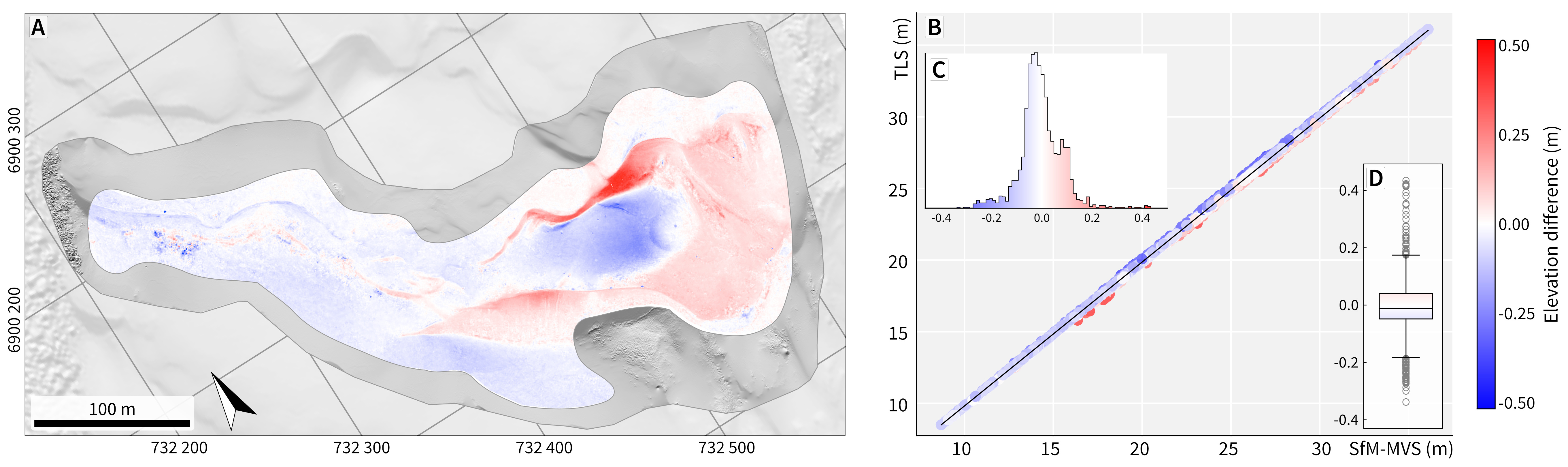
Figure 6: Differences between TLS and SfM-MVS: A) Map of difference values (all pixels); B) Scatterplot; C) Histogram (bins=60); D) Boxplot. Data for B,C,D from a set of $2\text{~{}}000$ random pixels.

3.2 ALS and SfM-MVS

Besides a good correlation to the TLS DEM, the full SfM-MVS DEM (Fig. 7B) shows a good fit with elements of the landscape that didn’t experienced significant change between the surveys, such as the road bordering the dune field to west and southwest (in grey in Fig. 7C, indicating no elevation difference).

Comparison of the 2010 ALS and 2019 SfM-MVS DEMs was carried out based on: 1) descriptive statistics of the DEMs; 2) differences between the DEMs; 3) sand volume within an area and 4) displacement of dune crests.

Differences between the DEMs were calculated by subtracting the elevations of the ALS DcrestEM from the SfM-MVS DEM. Positive values represent areas where the SfM surface has higher elevations than the ALS one, and vice-versa.

The ALS and SfM-MVS DEMs (0.5 m resolution) and the differences between the two surfaces, are presented in Fig. 7. In the studied area, dunes are mainly barchanoids with lee side towards south west. Elevation reaches its highest ($\approx$58 m) in the southern portion, likely due the influence of an underlying palaeotopography (Giannini et al., 2007).

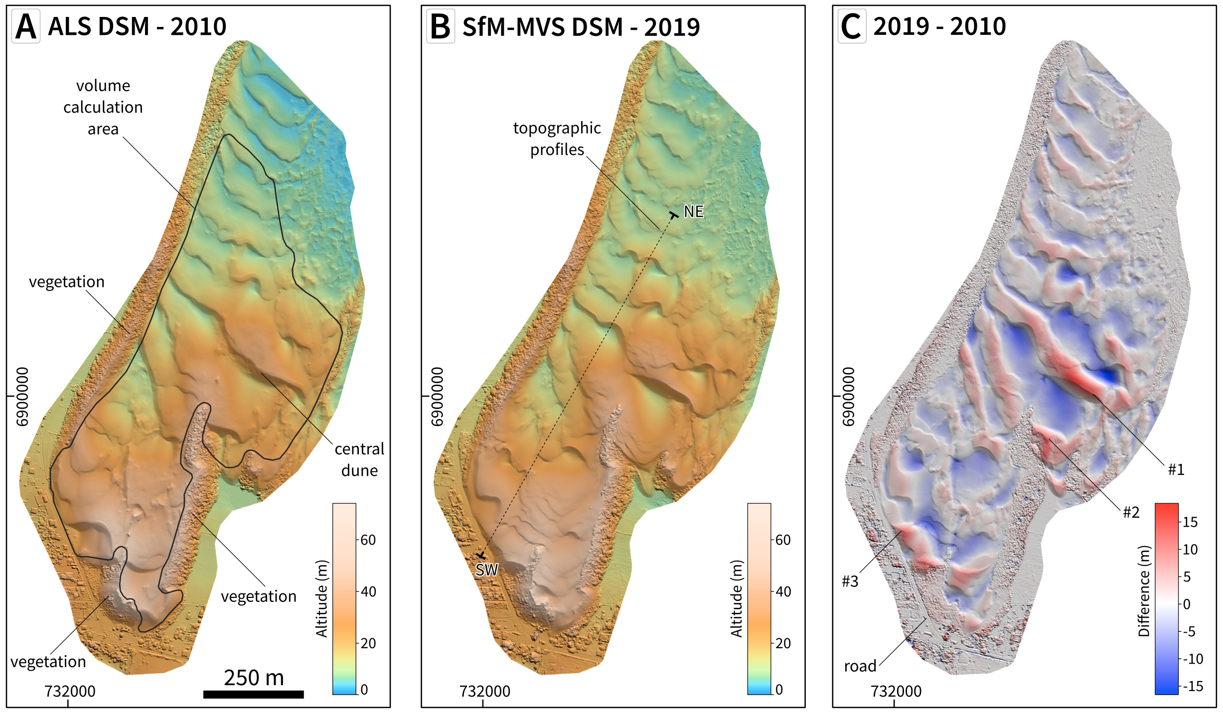
Figure 7: A) ALS DEM (2010), with volume calculation area polygon; B) SfM-MVS DEM (2019), with topographic profiles location; C) DEM of differences (2019-2010). Numbers in C are discussed in the text.

Descriptive statistics are presented in Table 3 and histograms of elevation values in Fig. 8. The DEM of differences between 2019 and 2010 DEMs is in Fig. 7C; positive values are in red and negative values in blue. Topographic profiles (location in Fig. 7B) are in Fig. 9.

The DEMs have similar values of maximum, standard deviation, skewness, kurtosis and quantiles. The SfM-MVS DEM shows slightly higher mean and minimum values. Elevation differences between the DEMs range from -16.95 m to +23.15 m, with mean and median of $\approx$0.0 ms. Some notable differences are indicated as #1,#2 and #3 in Fig. 7C: #1 marks the highest positive difference (where the SfM-MVS surface is above the ALS), related to the migration of a large ‘central dune’ with accumulation of sand towards a vegetated ridge in #2; #3 shows the migration of the dune field over the road. In this place, the town hall needs to remove the sand periodically to keep the road open.

Table 3: Descriptive statistics of the ALS, SfM-MVS DEMs and of differences between the two surfaces.

	min	max	mean	median	std.dev.	skewness	kurtosis	25%quant.	75%quant.
ALS	2.69	58.88	21.34	20.65	11.59	0.51	-0.41	11.64	28.77
SfM-MVS	2.89	58.63	21.64	20.67	11.66	0.45	-0.57	11.63	29.40
Diff.	-16.95	23.15	0.31	0.39	3.48	0.16	2.77	-1.26	1.80

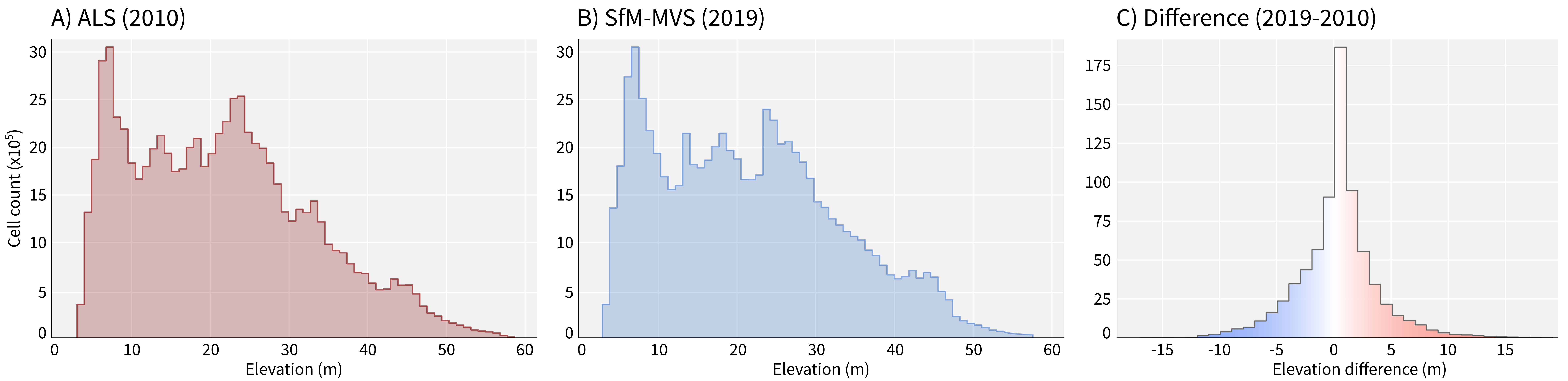
Figure 8: Histograms: A) ALS DEM (bins=60); SfM-MVS DEM (bins=60); C) DEM of differences (bins=40).

The polygon for volume calculation encloses only unvegetated areas in both surveys (see Fig. 7A). Using the ALS and SfM DEMs with 0.5 m resolution, the calculated sand volumes were $9\text{~{}}035\text{~{}}115.45$ ${\mathrm{m}}^{3}$ for 2010 and $9\text{~{}}010\text{~{}}844.95$ ${\mathrm{m}}^{3}$ for 2019 (a decrease of $24\text{~{}}270.50$ ${\mathrm{m}}^{3}$ or 0.2%).

Dune crest displacement lines drawn over the DEMs (see Fig. 3) yielded a mean azimuth of $215.5\mathrm{°}$ and mean length of $\approx$44.5 m (mean: 44.3 m, median: 44.7 m, see Supplemental Material for statistical analysis of azimuth and length).

A mean length of 44.5 m in 9 years corresponds to a dune migration rate of $\approx$5 m/year. We consider these rates to be in agreement with rates of 6-7 m/year from Mendes and Giannini (2015) and Mendes et al. (2015), which were derived from interpretation of historical aerial photographs and satellite images with coarser spatial resolution.

Topographic profiles (Fig. 9) illustrate dune movement from 2010 to 2019, with migration of the lee side and relatively less change over the stoss side of large compound dunes.

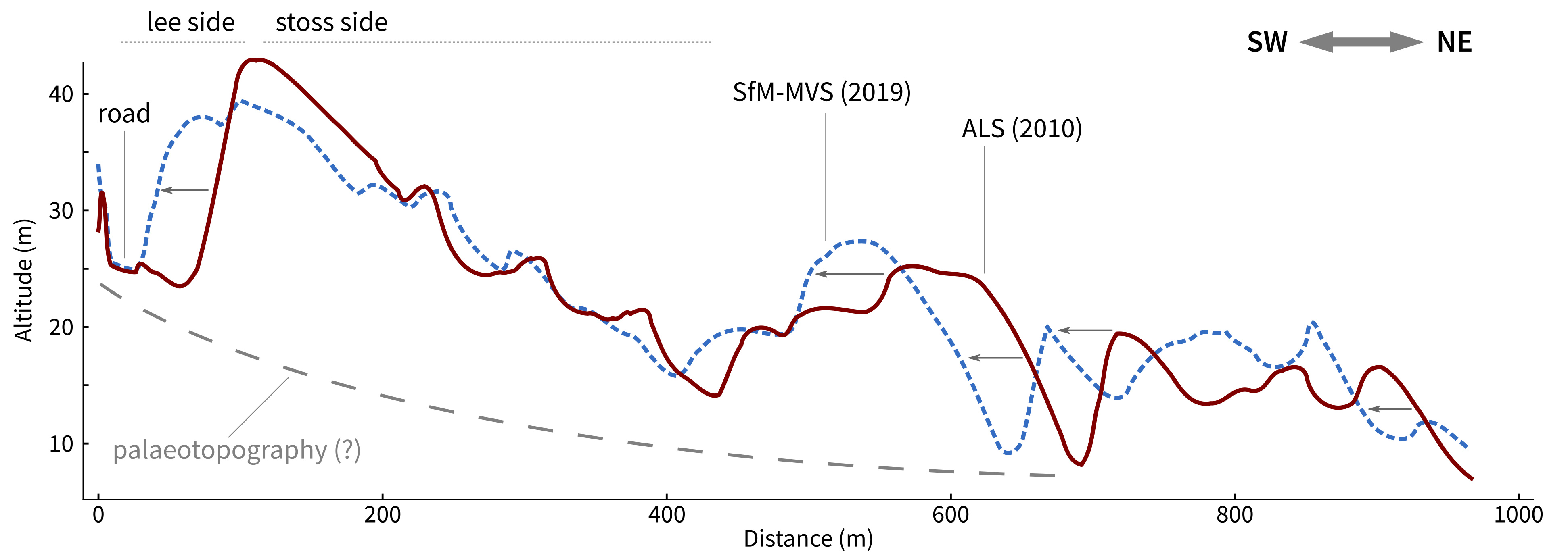
Figure 9: Topographic profiles across the dune field (location in Fig. 7B.)

4 Discussions and Conclusions

In this work we presented an evaluation of SfM-MVS in high-resolution topographic modelling of coastal sand dunes.

Although sand dunes are commonly regarded as a challenge to traditional photogrammetry due their homogeneous texture and spectral response, yielding poor results in image matching (Baltsavias, 1999), recent literature on close-range photogrammetry/SfM-MVS of coastal areas report good results in surface reconstruction (Gonçalves and Henriques, 2015; Gonçalves et al., 2018; Duffy et al., 2018; Laporte-Fauret et al., 2019; van Puijenbroek et al., 2017; Guisado-Pintado et al., 2019; Pitman et al., 2019).

In this research, image matching was successful in all areas of the survey due the presence of superficial features (footprints and sandboard tracks) and visibility of the sedimentary stratification, highlighted by heavy minerals (Fig. 2C).

One factor that positively influenced the RPA survey was the weather. A cloudy sky provided a diffuse illumination, without ‘hard’ shadows, and the scattered light rain ensured that the sand was humid, without the presence of a layer of loose sand over the dunes, which would mask the stratifications and other features in the photos (Guisado-Pintado et al., 2019).

We believe that the lack of texture in aerial photographs and satellite images is more related to ground resolution (i.e., pixel size) than the spectral or morphological characteristics of aeolian dunes, as a pixel area of one square metre can be enough to ‘average-out’ small textural features and prevent good image matching. This is an issue to be seen in the context of the everlasting matter of scale in remote sensing and geomorphometry: pixel size vs. spatial structure (size) of landforms (e.g., Woodcock and Strahler, 1987; Wood, 1996; Gallant and Hutchinson, 1997; Goodchild and Quattrochi, 1997; Marceau and Hay, 1999; Hengl, 2006; Kamal et al., 2014). Large continental dunes, for instance, have been successfully modelled with 30 m-resolution images from Landsat and ASTER (Levin et al., 2004; Bullard et al., 2011).

To validate the use of an SfM-MVS DEM, a TLS DEM was used as reference for altimetric accuracy. The comparison resulted in RMSE of 0.08 m and MAE of 0.06 m. The TLS DEM has a smooth appearance, with well-marked dune crests and vegetated areas, while the SfM-MVS DEM shows a small-scale roughness that hinders visual identification of small features such as footprints.

Although it does not influence the comparison with ALS data, this roughness can be an issue if the objective of the research is the classification of landforms based on geomorphometric parameters, such as the identification of dune crests based on surface curvature (Mitasova et al., 2005b; Hardin et al., 2014). The FPD de-noise algorithm (Lindsay et al., 2019) was applied to the SfM-MVS DEM with good results in terms of surface smoothing, without any significant changes in descriptive statistics and error metrics.

Dune crests interpreted from the ALS DEM were compared to crests from the SfM-MVS DEM and resulted in a migration rate of $\approx$5 m/year, in good agreement with rates derived from satellite images and historical aerial photographs of the same area (Mendes and Giannini, 2015; Mendes et al., 2015).

Volumes calculated from the ALS and SfM-MVS DEMs show a difference of 0.2% between 2010 and 2019. Such small variation is within reported uncertainties for SfM-MVS reconstructions (Draeyer and Strecha, 2014; Rhodes, 2017; Gupta and Shukla, 2018) and may be related to the the installation of sand fences to promote dune stabilization and the constant removal of sand from the road in front of the dune field (Fig. 10). Future studies can explore the spatial distribution of differences in the DEMs to evaluate the sedimentary budget (influx$-$efflux) of the dune field (Sankey et al., 2018a, b; Kasprak et al., 2019).

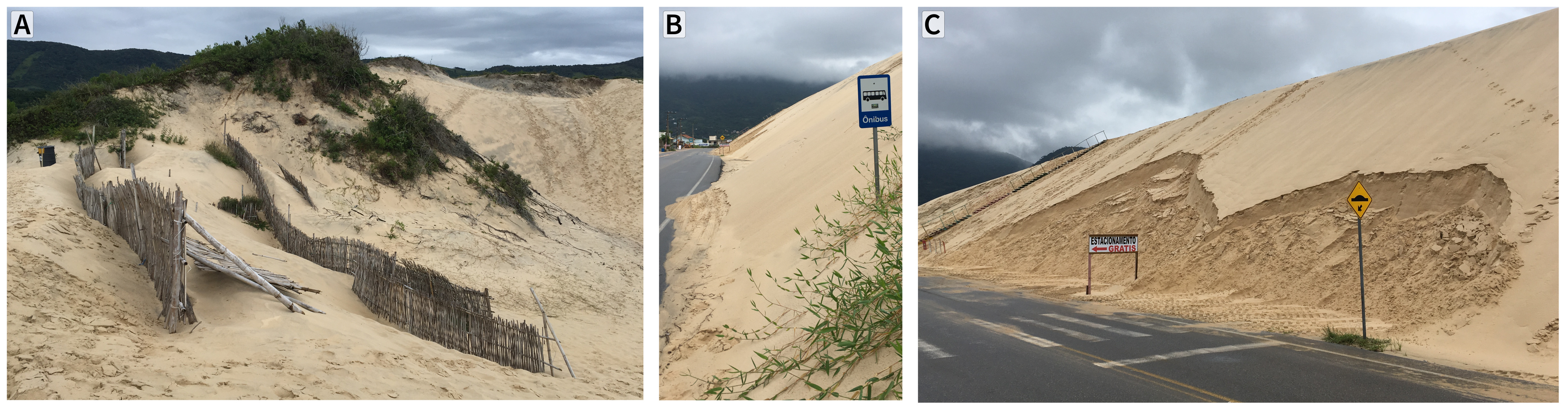
Figure 10: A) Sand fences installed to promote dune stabilization; B, C) Front of the dune field showing migration over road and signs. Location of photos on Fig. 2B.

When comparing these different approaches to aeolian dune surface modelling (ALS, TLS and SfM-MVS) we must consider not only the accuracy of final products (DEMs), but also the time required to acquire the data and process it to a GIS-ready format.

ALS might be acquired in little time, but it is by far the most expensive, imposing a serious constrain on repeated surveys, especially for researchers in developing countries or without access to state-funded coastal monitoring programs.

TLS has an intermediate cost of acquisition (since the equipment can be rented and operated by the research team) but it demands more fieldwork and more processing time. In our case we needed three days for the TLS survey and around three weeks of full-time work to produce a DEM of $\approx$$80\text{~{}}400$$\mathrm{m}^{2}$.

SfM-MVS has gained attention recently for being a low-cost solution with fast and reliable results (James et al., 2019). We were able to cover $\approx$$740\text{~{}}900$$\mathrm{m}^{2}$ with six RPA missions in under three hours. Processing time in a medium-range workstation (i.e., i7 processor, 64 GB RAM, dedicated GPU) was $\approx$13 hours. This makes it an excellent method for 3D modelling and continuous monitoring of coastal dunes.

One strength of the ALS over TLS and SfM-MVS is the possibility of removing the vegetation based on the laser returns or waveform (Brovelli and Cannata, 2004; Evans and Hudak, 2007; Khosravipour et al., 2016), although new methods are being developed for single-return point clouds (Guarnieri et al., 2009; Coveney et al., 2010; Coveney and Stewart Fotheringham, 2011; Montreuil et al., 2013; Pijl et al., 2020) that have been used in coastal environments with good results (Guisado-Pintado et al., 2019).

Another aspect to be considered is the weather. Dry and hot conditions will favour the presence of white sand patches, which can affect image matching and the 3D reconstruction. While clear sunny days might be seen by many as ideal conditions for fieldwork, flying the RPA with cloudy skies and after a light rain can be worthwhile due the scattered light and visibility of the dune’s superficial features.

Computer Code Availability

Jupyter notebooks and associated data files (shapefiles and csv files) are available on GitHub (https://github.com/CarlosGrohmann/scripts_papers/tree/master/garopaba_als_sfm_tls) and Zenodo (https://doi.org/10.5281/zenodo.3476779). The notebooks are based on Python 3.6 and depend on the following libraries: numpy, scipy.stats, matplotlib, pandas, seaborn, rasterio, xarray, statsmodels, osgeo.ogr, pygrass and whiteboxtools.

Data Availability

The point cloud datasets used in this study are available via the OpenTopography Facility (Crosby et al., 2011; Krishnan et al., 2011). The following datasets were used: OpenTopography ID OT.032013.32722.1 (ALS – Grohmann, 2010; Grohmann and Sawakuchi, 2013), OTDS.072019.32722.1 (SfM – Grohmann, 2019), OTDS.102019.32722.1 (TLS – Grohmann et al., 2019).

References

- Angulo et al. (2006) Angulo, R., Lessa, G., Souza, M., 2006. A critical review of mid-to late-Holocene sea-level fluctuations on the eastern Brazilian coastline. Quaternary Science Reviews 25, 486–506.
- Baade and Schmullius (2016) Baade, J., Schmullius, C., 2016. TanDEM-X IDEM precision and accuracy assessment based on a large assembly of differential GNSS measurements in Kruger National Park, South Africa. ISPRS Journal of Photogrammetry and Remote Sensing 119, 496 – 508. doi:https://doi.org/10.1016/j.isprsjprs.2016.05.005.
- Baltsavias (1999) Baltsavias, E.P., 1999. A comparison between photogrammetry and laser scanning. ISPRS Journal of Photogrammetry and Remote Sensing 54, 83–94.
- Bañón et al. (2019) Bañón, L., Pagán, J.I., López, I., Banon, C., Aragonés, L., 2019. Validating UAS-Based Photogrammetry with Traditional Topographic Methods for Surveying Dune Ecosystems in the Spanish Mediterranean Coast. Journal of Marine Science and Engineering 7. doi:10.3390/jmse7090297.
- Barash (2002) Barash, D., 2002. Fundamental relationship between bilateral filtering, adaptive smoothing, and the nonlinear diffusion equation. IEEE Transactions on Pattern Analysis and Machine Intelligence 24, 844–847. doi:10.1109/TPAMI.2002.1008390.
- Barnes (2010) Barnes, N., 2010. Publish your computer code: it is good enough. Nature 467, 753. doi:10.1038/467753a.
- Baughman et al. (2018) Baughman, C.A., Jones, B.M., Bodony, K.L., Mann, D.H., Larsen, C.F., Himelstoss, E., Smith, J., 2018. Remotely Sensing the Morphometrics and Dynamics of a Cold Region Dune Field Using Historical Aerial Photography and Airborne LiDAR Data. Remote Sensing 10. doi:10.3390/rs10050792.
- Berti et al. (2013) Berti, M., Corsini, A., Daehne, A., 2013. Comparative analysis of surface roughness algorithms for the identification of active landslides. Geomorphology 182, 1–18. URL: http://www.sciencedirect.com/science/article/pii/S0169555X12004862, doi:10.1016/j.geomorph.2012.10.022.
- Bhadra et al. (2019) Bhadra, B.K., Rehpade, S.B., Meena, H., Srinivasa Rao, S., 2019. Analysis of Parabolic Dune Morphometry and Its Migration in Thar Desert Area, India, using High-Resolution Satellite Data and Temporal DEM. Journal of the Indian Society of Remote Sensing URL: https://doi.org/10.1007/s12524-019-01050-, doi:10.1007/s12524-019-01050-1.
- Bourke et al. (2010) Bourke, M.C., Lancaster, N., Fenton, L.K., Parteli, E.J., Zimbelman, J.R., Radebaugh, J., 2010. Extraterrestrial dunes: An introduction to the special issue on planetary dune systems. Geomorphology 121, 1 – 14. URL: http://www.sciencedirect.com/science/article/pii/S0169555X10001868, doi:10.1016/j.geomorph.2010.04.007.
- Brovelli and Cannata (2004) Brovelli, M.A., Cannata, M., 2004. Digital terrain model reconstruction in urban areas from airborne laser scanning data: the method and an example for Pavia (northern Italy). Computers & Geosciences 30, 325–331. doi:10.1016/j.cageo.2003.07.004.
- Brovelli et al. (2004) Brovelli, M.A., Cannata, M., Longoni, U.M., 2004. LIDAR Data Filtering and DTM Interpolation Within GRASS. Transactions in GIS 8, 155–174. doi:10.1111/j.1467-9671.2004.00173.x.
- Bullard et al. (2011) Bullard, J.E., White, K., Livingstone, I., 2011. Morphometric analysis of aeolian bedforms in the Namib Sand Sea using ASTER data. Earth Surface Processes and Landforms 36, 1534–1549. doi:10.1002/esp.2189.
- Casella et al. (2020) Casella, E., Drechsel, J., Winter, C., Benninghoff, M., Rovere, A., 2020. Accuracy of sand beach topography surveying by drones and photogrammetry. Geo-Marine Letters doi:10.1007/s00367-020-00638-8.
- Clemmensen et al. (2007) Clemmensen, L.B., Bjørnsen, M., Murray, A., Pedersen, K., 2007. Formation of aeolian dunes on Anholt, Denmark since AD 1560: A record of deforestation and increased storminess. Sedimentary Geology 199, 171 – 187. URL: http://www.sciencedirect.com/science/article/pii/S0037073807000486, doi:10.1016/j.sedgeo.2007.01.025.
- Conlin et al. (2018) Conlin, M., Cohn, N., Ruggiero, P., 2018. A Quantitative Comparison of Low-Cost Structure from Motion (SfM) Data Collection Platforms on Beaches and Dunes. Journal of Coastal Research 34, 1341–1357. doi:10.2112/JCOASTRES-D-17-00160.1.
- Coveney et al. (2010) Coveney, S., Fotheringham, A.S., Charlton, M., McCarthy, T., 2010. Dual-scale validation of a medium-resolution coastal DEM with terrestrial LiDAR DSM and GPS. Computers & Geosciences 36, 489 – 499. doi:https://doi.org/10.1016/j.cageo.2009.10.003.
- Coveney and Stewart Fotheringham (2011) Coveney, S., Stewart Fotheringham, A., 2011. Terrestrial laser scan error in the presence of dense ground vegetation. The Photogrammetric Record 26, 307–324. doi:10.1111/j.1477-9730.2011.00647.x.
- Crosby et al. (2011) Crosby, C.J., Arrowsmith, R.J., Nandigam, V., Baru, C., 2011. Geoinformatics. Cambridge University Press. chapter Online access and processing of LiDAR topography data. p. 251–265. doi:10.1017/CBO9780511976308.017.
- Dillenburg et al. (2006) Dillenburg, S., Tomazelli, L., Hesp, P., Barboza, E., Clerot, L., da Silva, D., 2006. Stratigraphy and Evolution of a Prograded Transgressive Dunefield Barrier in Southern Brazil. Journal of Coastal Research , 132–135URL: http://www.jstor.org/stable/25741548.
- Dong (2015) Dong, P., 2015. Automated measurement of sand dune migration using multi-temporal lidar data and GIS. International Journal of Remote Sensing 36, 5426–5447. URL: https://doi.org/10.1080/01431161.2015.1093192, doi:10.1080/01431161.2015.1093192, arXiv:https://doi.org/10.1080/01431161.2015.1093192.
- Draeyer and Strecha (2014) Draeyer, B., Strecha, C., 2014. White paper: How accurate are UAV surveying methods. Pix4D White Paper URL: https://pdfs.semanticscholar.org/0dd7/1fdcaefbc22e54f2ba7f8bb0fa8af33edb4c.pdf.
- Duffy et al. (2018) Duffy, J.P., Shutler, J.D., Witt, M.J., DeBell, L., Anderson, K., 2018. Tracking Fine-Scale Structural Changes in Coastal Dune Morphology Using Kite Aerial Photography and Uncertainty-Assessed Structure-from-Motion Photogrammetry. Remote Sensing 10. URL: https://www.mdpi.com/2072-4292/10/9/1494, doi:10.3390/rs10091494.
- Evans and Hudak (2007) Evans, J.S., Hudak, A.T., 2007. A Multiscale Curvature Algorithm for Classifying Discrete Return LiDAR in Forested Environments. Geoscience and Remote Sensing, IEEE Transactions in 45, 1029–1038. doi:10.1109/TGRS.2006.890412.
- Fabbri et al. (2017) Fabbri, S., Giambastiani, B.M., Sistilli, F., Scarelli, F., Gabbianelli, G., 2017. Geomorphological analysis and classification of foredune ridges based on Terrestrial Laser Scanning (TLS) technology. Geomorphology 295, 436 – 451. doi:https://doi.org/10.1016/j.geomorph.2017.08.003.
- FARO Technologies Inc. (2013) FARO Technologies Inc., 2013. User Manual for the Focus3D 20/120 and S 20/120. URL: https://knowledge.faro.com/Hardware/3D_Scanners/Focus/User_Manual_for_the_Focus3D_20-120_and_S_20-120?mt-learningpath=focus3d_20-120_downloads. last access: 01/Jul/2019.
- Feagin et al. (2014) Feagin, R.A., Williams, A.M., Popescu, S., Stukey, J., Washington-Allen, R.A., 2014. The Use of Terrestrial Laser Scanning (TLS) in Dune Ecosystems: The Lessons Learned. Journal of Coastal Research , 111–119URL: https://doi.org/10.2112/JCOASTRES-D-11-00223.1, doi:10.2112/JCOASTRES-D-11-00223.1.
- Finkel (1961) Finkel, H.J., 1961. The movement of barchan dunes measured by aerial photogrammetry. Photogram Eng 27, 439–444.
- Fisher (1993) Fisher, N.I., 1993. Statistical Analysis of Circular Data. Cambridge Univ. Press, Cambridge.
- Forlani et al. (2018) Forlani, G., Dall’Asta, E., Diotri, F., Cella, U.M.d., Roncella, R., Santise, M., 2018. Quality Assessment of DSMs Produced from UAV Flights Georeferenced with On-Board RTK Positioning. Remote Sensing 10. URL: https://www.mdpi.com/2072-4292/10/2/311, doi:10.3390/rs10020311.
- Fryberger and Dean (1979) Fryberger, S.G., Dean, G., 1979. A Study of Global Sand Seas. U.S. Geological Survey. volume Prof. Paper 1052. chapter Dune forms and wind regime. pp. 137–169.
- Gallant (2011) Gallant, J., 2011. Adaptive smoothing for noisy DEMs, in: Hengl, T., Evans, I.S., Wilson, J.P., Gould, M. (Eds.), Geomorphometry 2011, Redlands, CA. pp. 37–40.
- Gallant and Hutchinson (1997) Gallant, J., Hutchinson, M., 1997. Scale dependence in terrain analysis. Mathematics and Computers in Simulation 43, 313–322.
- Garcin et al. (2019) Garcin, M., Desmazes, F., Nicolae‐Lerma, A., Gouguet, L., Metereau, V., 2019. Contribution of Lightweight Revolving Laser Scanner, HiRes UAV LiDARs and photogrammetry for characterization of coastal aeolian morphologies. preprint hosted by ResearchGate doi:10.13140/RG.2.2.30916.99207.
- Gaylord et al. (2001) Gaylord, D.R., Foit, F.F., Schatz, J.K., Coleman, A.J., 2001. Smith Canyon dune field, Washington, U.S.A: relation to glacial outburst floods, the Mazama eruption, and Holocene paleoclimate. Journal of Arid Environments 47, 403 – 424. doi:10.1006/jare.2000.0731.
- GDAL Development Team (2019) GDAL Development Team, 2019. GDAL - Geospatial Data Abstraction Library, Version 2.4.1. Open Source Geospatial Foundation. Available at http://gdal.osgeo.org, last access 20-July-2019,.
- Gesch et al. (2016) Gesch, D.B., Oimoen, M.J., Danielson, J.J., Meyer, D., 2016. Validation of the ASTER Global Digital Elevation Model version 3 over the conterminous United States. International Archives of the Photogrammetry, Remote Sensing and Spatial Information Sciences XLI-B4, 143–148. URL: http://pubs.er.usgs.gov/publication/70175051.
- Giannini et al. (2007) Giannini, P.C.F., Sawakuchi, A.O., Martinho, C.T., Tatumi, S.H., 2007. Eolian depositional episodes controlled by Late Quaternary relative sea level changes on the Imbituba-Laguna coast (southern Brazil). Marine Geology 237, 143–168.
- Gillies et al. (2013–) Gillies, S., et al., 2013–. Rasterio: geospatial raster I/O for Python programmers. URL: https://github.com/mapbox/rasterio.
- Gonçalves et al. (2018) Gonçalves, G.R., Pérez, J.A., Duarte, J., 2018. Accuracy and effectiveness of low cost UASs and open source photogrammetric software for foredunes mapping. International Journal of Remote Sensing 39, 5059–5077. doi:10.1080/01431161.2018.1446568, arXiv:https://doi.org/10.1080/01431161.2018.1446568.
- Gonçalves and Henriques (2015) Gonçalves, J., Henriques, R., 2015. UAV photogrammetry for topographic monitoring of coastal areas. ISPRS Journal of Photogrammetry and Remote Sensing 104, 101 – 111. doi:10.1016/j.isprsjprs.2015.02.009.
- Goodchild and Quattrochi (1997) Goodchild, M., Quattrochi, D., 1997. Scale in Remote Sensing and GIS. CRC Press. chapter Introduction: scale, multiscaling, remote sensing and GIS. pp. 1–12.
- GRASS Development Team (2019) GRASS Development Team, 2019. Geographic Resources Analysis Support System (GRASS GIS) Software, Version 7.6. Open Source Geospatial Foundation. URL: http://grass.osgeo.org.
- Grohmann (2004) Grohmann, C.H., 2004. Morphometric analysis in Geographic Information Systems: applications of free software GRASS and R. Computers & Geosciences 30, 1055–1067. doi:10.1016/j.cageo.2004.08.002.
- Grohmann (2010) Grohmann, C.H., 2010. Coastal Dune Fields of Garopaba and Vila Nova, Santa Catarina State, Brazil. Airborne LiDAR. Data provided by FAPESP grant #2009/17675-5, distributed by OpenTopography. doi:10.5069/G9DN430Z. oT Collection ID: OT.032013.32722.1.
- Grohmann (2018) Grohmann, C.H., 2018. Evaluation of TanDEM-X DEMs on selected Brazilian sites: Comparison with SRTM, ASTER GDEM and ALOS AW3D30. Remote Sensing of Environment 212, 121 – 133. doi:10.1016/j.rse.2018.04.043.
- Grohmann (2019) Grohmann, C.H., 2019. Garopaba Dune Field, Santa Catarina State, Brazil. SfM-MVS point cloud. Data provided by FAPESP grant #2016/06628-0, distributed by OpenTopography. doi:10.5069/G9DV1H19. opentopoID: OTDS.072019.32722.1.
- Grohmann et al. (2019) Grohmann, C.H., Garcia, G.P.B., Affonso, A.A., Albuquerque, R.W., 2019. Garopaba Dune Field, Santa Catarina State, Brazil. TLS point cloud. Data provided by FAPESP grant #2016/06628-0, distributed by OpenTopography. doi:10.5069/G9CN7228. opentopoID: OTDS.102019.32722.1.
- Grohmann and Hargitai (2014) Grohmann, C.H., Hargitai, H., 2014. Surface Roughness, in: Encyclopedia of Planetary Landforms. Springer New York, pp. 1–4. doi:10.1007/978-1-4614-9213-9_633-1.
- Grohmann and Riccomini (2009) Grohmann, C.H., Riccomini, C., 2009. Comparison of roving-window and search-window techniques for characterising landscape morphometry. Computers & Geosciences 35, 2164–2169. doi:10.1016/j.cageo.2008.12.014.
- Grohmann and Sawakuchi (2013) Grohmann, C.H., Sawakuchi, A.O., 2013. Influence of cell size on volume calculation using digital terrain models: A case of coastal dune fields. Geomorphology 180-181, 130–136. doi:10.1016/j.geomorph.2012.09.012.
- Grohmann et al. (2010) Grohmann, C.H., Smith, M.J., Riccomini, C., 2010. Multiscale Analysis of Topographic Surface Roughness in the Midland Valley, Scotland. Geoscience and Remote Sensing, IEEE Transactions on 49, 1200–1213. doi:10.1109/TGRS.2010.2053546.
- Guarnieri et al. (2009) Guarnieri, A., Vettore, A., Pirotti, F., Menenti, M., Marani, M., 2009. Retrieval of small-relief marsh morphology from Terrestrial Laser Scanner, optimal spatial filtering, and laser return intensity. Geomorphology 113, 12 – 20. doi:https://doi.org/10.1016/j.geomorph.2009.06.005. understanding earth surface processes from remotely sensed digital terrain models.
- Guisado-Pintado et al. (2019) Guisado-Pintado, E., Jackson, D., Rogers, D., 2019. 3D mapping efficacy of a drone and terrestrial laser scanner over a temperate beach-dune zone. Geomorphology 328, 157–172. doi:10.1016/j.geomorph.2018.12.013.
- Gupta and Shukla (2018) Gupta, S.K., Shukla, D.P., 2018. Application of drone for landslide mapping, dimension estimation and its 3D reconstruction. Journal of the Indian Society of Remote Sensing 46, 903–914. doi:10.1007/s12524-017-0727-1.
- Hardin et al. (2014) Hardin, E., Mitasova, H., Tateosian, L., Overton, M., 2014. GIS-based Analysis of Coastal Lidar Time-Series. Springer New York. doi:10.1007/978-1-4939-1835-5.
- Harwin et al. (2015) Harwin, S., Lucieer, A., Osborn, J., 2015. The Impact of the Calibration Method on the Accuracy of Point Clouds Derived Using Unmanned Aerial Vehicle Multi-View Stereopsis. Remote Sensing 7, 11933–11953. URL: https://www.mdpi.com/2072-4292/7/9/11933, doi:10.3390/rs70911933.
- Hayes (2018) Hayes, A., 2018. Dunes across the solar system. Science 360, 960–961. doi:10.1126/science.aat7488. cited By 1.
- Hayward et al. (2007) Hayward, R., Mullins, K., Fenton, L., Hare, T., Titus, T., Bourke, M., Colaprete, A., Christensen, P., 2007. Mars global digital dune database and initial science results. Journal of Geophysical Research 112, E11007. doi:10.1029/2007JE002943.
- Hebeler and Purves (2009) Hebeler, F., Purves, R.S., 2009. The influence of elevation uncertainty on derivation of topographic indices. Geomorphology 111, 4–16.
- Hengl (2006) Hengl, T., 2006. Finding the right pixel size. Computers and Geosciences 32, 1283–1298.
- Hengl and Reuter (2008) Hengl, T., Reuter, H.I., 2008. Geomorphometry: Concepts, Software, Applications. volume 33 of Developments in Soil Science. Elsevier, Amsterdam.
- Hesp et al. (2007) Hesp, P., Abreu de Castilhos, J., Miot da Silva, G., Dillenburg, S., Martinho, C.T., Aguiar, D., Fornari, M., Fornari, M., Antunes, G., 2007. Regional wind fields and dunefield migration, southern Brazil. Earth Surface Processes and Landforms 32, 561–573. doi:10.1002/esp.1406.
- Hinthorne (1988) Hinthorne, J., 1988. r.volume GRASS-GIS module. URL: http://grass.osgeo.org/grass64/manuals/html64_user/r.volume.html. [accessed 05 December 2011].
- Hoover et al. (2018) Hoover, R.H., Gaylord, D.R., Cooper, C.M., 2018. Dune mobility in the St. Anthony Dune Field, Idaho, USA: Effects of meteorological variables and lag time. Geomorphology 309, 29 – 37. doi:10.1016/j.geomorph.2018.02.018.
- Hugenholtz and Barchyn (2010) Hugenholtz, C.H., Barchyn, T.E., 2010. Spatial analysis of sand dunes with a new global topographic dataset: new approaches and opportunities. Earth Surface Processes and Landforms 35, 986–992. URL: http://dx.doi.org/10.1002/esp.2013, doi:10.1002/esp.2013.
- Hunter (2007) Hunter, J.D., 2007. Matplotlib: A 2D graphics environment. Computing In Science & Engineering 9, 90–95. doi:10.1109/MCSE.2007.55.
- Isenburg (2019) Isenburg, M., 2019. LAStools - efficient LiDAR processing software (version 190623, unlicensed). Obtained from http://rapidlasso.com/LAStools.
- James et al. (2019) James, M.R., Chandler, J.H., Eltner, A., Fraser, C., Miller, P.E., Mills, J.P., Noble, T., Robson, S., Lane, S.N., 2019. Guidelines on the use of structure-from-motion photogrammetry in geomorphic research. Earth Surface Processes and Landforms 44, 2081–2084. doi:10.1002/esp.4637, arXiv:https://onlinelibrary.wiley.com/doi/pdf/10.1002/esp.4637.
- James and Robson (2014) James, M.R., Robson, S., 2014. Mitigating systematic error in topographic models derived from UAV and ground-based image networks. Earth Surface Processes and Landforms 39, 1413–1420. URL: http://dx.doi.org/10.1002/esp.3609, doi:10.1002/esp.3609. eSP-14-0032.R2.
- Judge et al. (2000) Judge, E.K., Courtney, M.G., Overton, M.F., 2000. Topographic analysis of dune volume and position, Jockey’s Ridge State Park, North Carolina. Shore and Beach 68, 19–24.
- Kamal et al. (2014) Kamal, M., Phinn, S., Johansen, K., 2014. Characterizing the Spatial Structure of Mangrove Features for Optimizing Image-Based Mangrove Mapping. Remote Sensing 6, 984–1006. doi:10.3390/rs6020984.
- Kasprak et al. (2019) Kasprak, A., Bransky, N.D., Sankey, J.B., Caster, J., Sankey, T.T., 2019. The effects of topographic surveying technique and data resolution on the detection and interpretation of geomorphic change. Geomorphology 333, 1 – 15. doi:https://doi.org/10.1016/j.geomorph.2019.02.020.
- Khosravipour et al. (2016) Khosravipour, A., Skidmore, A.K., Isenburg, M., 2016. Generating spike-free digital surface models using LiDAR raw point clouds: A new approach for forestry applications. International Journal of Applied Earth Observation and Geoinformation 52, 104 – 114. doi:http://dx.doi.org/10.1016/j.jag.2016.06.005.
- Kluyver et al. (2016) Kluyver, T., Ragan-Kelley, B., Pérez, F., Granger, B., Bussonnier, M., Frederic, J., Kelley, K., Hamrick, J., Grout, J., Corlay, S., Ivanov, P., Avila, D., Abdalla, S., Willing, C., 2016. Positioning and Power in Academic Publishing: Players, Agents and Agendas. IOS Press. chapter Jupyter Notebooks – a publishing format for reproducible computational workflows. pp. 87 – 90. doi:10.3233/978-1-61499-649-1-87.
- Kreslavsly and Bondarenko (2017) Kreslavsly, M.A., Bondarenko, N.V., 2017. Aeolian sand transport and aeolian deposits on Venus: A review. Aeolian Research 26, 29–46. doi:10.1016/j.aeolia.2016.06.001. cited By 4.
- Krishnan et al. (2011) Krishnan, S., Crosby, C., Nandigam, V., Phan, M., Cowart, C., Baru, C., Arrowsmith, R., 2011. OpenTopography: a services oriented architecture for community access to LIDAR topography, in: Proceedings of the 2nd International Conference on Computing for Geospatial Research & Applications, ACM, New York, NY, USA. pp. 7:1–7:8. doi:10.1145/1999320.1999327.
- Łabuz (2016) Łabuz, T.A., 2016. A review of field methods to survey coastal dunes—experience based on research from South Baltic coast. Journal of Coastal Conservation 20, 175–190. doi:10.1007/s11852-016-0428-x.
- Laporte-Fauret et al. (2019) Laporte-Fauret, Q., Marieu, V., Castelle, B., Michalet, R., Bujan, S., Rosebery, D., 2019. Low-Cost UAV for High-Resolution and Large-Scale Coastal Dune Change Monitoring Using Photogrammetry. Journal of Marine Science and Engineering 7. doi:10.3390/jmse7030063.
- Lee et al. (2019) Lee, Y.K., Eom, J., Do, J.D., amd Joo-Hyung Ryu, B.J.K., 2019. Shoreline Movement Monitoring and Geomorphologic Changes of Beaches Using Lidar and UAVs Images on the Coast of the East Sea, Korea. Journal of Coastal Research 90, 409 – 414 – 6. doi:10.2112/SI90-052.1.
- Levin (2011) Levin, N., 2011. Climate-driven changes in tropical cyclone intensity shape dune activity on Earth’s largest sand island. Geomorphology 125, 239 – 252. URL: http://www.sciencedirect.com/science/article/pii/S0169555X10004149, doi:10.1016/j.geomorph.2010.09.021.
- Levin et al. (2004) Levin, N., Dor, B.E., Karnieli, A., 2004. Topographic information of sand dunes as extracted from shading effects using Landsat images. Remote Sensing of Environment 90, 190–209.
- Lindsay (2017) Lindsay, J.B., 2017. WhiteboxTools User Manual. Available online: https://jblindsay.github.io/wbt_book/preface.html (accessed on 01 march 2020).
- Lindsay et al. (2019) Lindsay, J.B., Francioni, A., Cockburn, J.M.H., 2019. LiDAR DEM Smoothing and the Preservation of Drainage Features. Remote Sensing 11. doi:10.3390/rs11161926.
- Livingstone et al. (2007) Livingstone, I., Wiggs, G.F., Weaver, C.M., 2007. Geomorphology of desert sand dunes: A review of recent progress. Earth-Science Reviews 80, 239 – 257. URL: http://www.sciencedirect.com/science/article/pii/S0012825206001449, doi:10.1016/j.earscirev.2006.09.004.
- Mancini et al. (2013) Mancini, F., Dubbini, M., Gattelli, M., Stecchi, F., Fabbri, S., Gabbianelli, G., 2013. Using unmanned aerial vehicles (UAV) for high-resolution reconstruction of topography: The structure from motion approach on coastal environments. Remote Sensing 5, 6880–6898. doi:10.3390/rs5126880.
- Marceau and Hay (1999) Marceau, D.J., Hay, G.J., 1999. Remote sensing contributions to the scale issue. Canadian journal of remote sensing 25, 357–366.
- Martinho et al. (2006) Martinho, C.T., Giannini, P.C.F., Sawakuchi, A.O., Hesp, P.A., 2006. Morphological and depositional facies of transgressive dunefields in the Imbituba-Jaguaruna region, Santa Catarina State. Journal of Coastal Research SI39, 143–168.
- Martinho et al. (2010) Martinho, C.T., Hesp, P.A., Dillenburg, S.R., 2010. Morphological and temporal variations of transgressive dunefields of the northern and mid-littoral Rio Grande do Sul coast, Southern Brazil. Geomorphology 117, 14 – 32. URL: http://www.sciencedirect.com/science/article/pii/S0169555X0900467X, doi:10.1016/j.geomorph.2009.11.002.
- McKinney (2011) McKinney, W., 2011. pandas: a Foundational Python Library for Data Analysis and Statistics, in: Python for High Performance and Scientific Computing, pp. 1–9.
- Mendes and Giannini (2015) Mendes, V.R., Giannini, P.C.F., 2015. Coastal dunefields of south Brazil as a record of climatic changes in the South American Monsoon System. Geomorphology 246, 22 – 34. doi:10.1016/j.geomorph.2015.05.034.
- Mendes et al. (2015) Mendes, V.R., Giannini, P.C.F., Guedes, C.C.F., DeWitt, R., de Abreu Andrade, H.A., 2015. Central Santa Catarina coastal dunefields chronology and their relation to relative sea level and climatic changes. Brazilian Journal of Geology 45, 79 – 95. doi:10.1590/2317-4889201530143.
- Mitasova et al. (2004) Mitasova, H., Drake, T.G., Bernstein, D., Harmon, R.S., 2004. Quantifying Rapid Changes in Coastal Topography using Modern Mapping Techniques and Geographic Information System. Environmental & Engineering Geoscience 10, 1–11. doi:10.2113/10.1.1.
- Mitasova et al. (2005a) Mitasova, H., Mitas, L., Harmon, R.S., 2005a. Simultaneous spline approximation and topographic analysis for lidar elevation data in open source GIS. IEEE Geoscience and Remote Sensing Letters 2, 375–379. doi:10.1109/LGRS.2005.848533.
- Mitasova et al. (2005b) Mitasova, H., Overton, M., Harman, R.S., 2005b. Geospatial analysis of a coastal sand dune field evolution: Jockey’s Ridge, North Carolina. Geomorphology 72, 204–221. doi:10.1016/j.geomorph.2005.06.001.
- Montreuil et al. (2013) Montreuil, A.L., Bullard, J., Chandler, J., 2013. Detecting Seasonal Variations in Embryo Dune Morphology Using a Terrestrial Laser Scanner. Journal of Coastal Research 65, 1313–1318. URL: https://doi.org/10.2112/SI65-222.1, doi:10.2112/SI65-222.1.
- Mosbrucker et al. (2016) Mosbrucker, A.R., Major, J.J., Spicer, K.R., Pitlick, J., 2016. Camera system considerations for geomorphic applications of SfM photogrammetry. Earth Surface Processes and Landforms , n/a–n/aURL: http://dx.doi.org/10.1002/esp.4066, doi:10.1002/esp.4066. eSP-14-0305.R3.
- Neteler et al. (2012) Neteler, M., Bowman, M.H., Landa, M., Metz, M., 2012. GRASS GIS: A multi-purpose open source GIS. Environmental Modelling & Software 31, 124–130. doi:10.1016/j.envsoft.2011.11.014.
- Nikolakopoulos et al. (2006) Nikolakopoulos, K.G., Kamaratakis, E.K., Chrysoulakis, N., 2006. SRTM vs. ASTER elevation products. Comparison for two regions in Crete, Grece. International Journal of Remote Sensing 27, 4819–4838.
- O’Dea et al. (2019) O’Dea, A., Brodie, K.L., Hartzell, P., 2019. Continuous Coastal Monitoring with an Automated Terrestrial Lidar Scanner. Journal of Marine Science and Engineering 7. doi:10.3390/jmse7020037.
- Oliphant (2006) Oliphant, T., 2006. Guide to NumPy. Trelgol Publishing. URL: http://www.tramy.us/.
- Pagán et al. (2019) Pagán, J., Bañón, L., López, I., Bañón, C., Aragonés, L., 2019. Monitoring the dune-beach system of Guardamar del Segura (Spain) using UAV, SfM and GIS techniques. Science of the Total Environment 687, 1034–1045. doi:10.1016/j.scitotenv.2019.06.186.
- Pardo-Pascual et al. (2005) Pardo-Pascual, J., García-Asenjo, L., Palomar-Vázquez, J., Garrigues-Talens, P., 2005. New Methods and Tools to analyze beach-dune system evolution using a Real-Time Kinematic Global Positioning System and Geographic Information Systems. Journal of Coastal Research , 34–39URL: http://www.jstor.org/stable/25737401.
- Pijl et al. (2020) Pijl, A., Bailly, J.S., Feurer, D., Maaoui, M.A.E., Boussema, M.R., Tarolli, P., 2020. TERRA: Terrain Extraction from elevation Rasters through Repetitive Anisotropic filtering. International Journal of Applied Earth Observation and Geoinformation 84, 101977. doi:https://doi.org/10.1016/j.jag.2019.101977.
- Pike (1995) Pike, R.J., 1995. Geomophometry – progress, practice, and prospect. Zeitschrift für Geomorphologie Suppl.-Bd. 101, 221–238.
- Pike et al. (2009) Pike, R.J., Evans, I.S., Hengl, T., 2009. Chapter 1. Geomorphometry: a brief guide, in: Hengl, T., Reuter, H.I. (Eds.), Geomorphometry: Concepts, Software, Applications. Elsevier, Amsterdam. volume 33 of Developments in Soil Science, pp. 3–30. doi:10.1016/S0166-2481(08)00001-9.
- Pitman et al. (2019) Pitman, S.J., Hart, D.E., Katurji, M.H., 2019. Application of UAV techniques to expand beach research possibilities: A case study of coarse clastic beach cusps. Continental Shelf Research 184, 44 – 53. doi:https://doi.org/10.1016/j.csr.2019.07.008.
- Potts et al. (2008) Potts, L.V., Akyilmaz, O., Braun, A., Shum, C.K., 2008. Multi-resolution dune morphology using Shuttle Radar Topography Mission (SRTM) and dune mobility from fuzzy inference systems using SRTM and altimetric data. International Journal of Remote Sensing 29, 2879–2901. URL: http://dx.doi.org/http://dx.doi.org/10.1080/01431160701408352, doi:http://dx.doi.org/http://dx.doi.org/10.1080/01431160701408352.
- van Puijenbroek et al. (2017) van Puijenbroek, M.E.B., Nolet, C., de Groot, A.V., Suomalainen, J.M., Riksen, M.J.P.M., Berendse, F., Limpens, J., 2017. Exploring the contributions of vegetation and dune size to early dune development using unmanned aerial vehicle (UAV) imaging. Biogeosciences 14, 5533–5549. doi:10.5194/bg-14-5533-2017.
- Python Software Foundation (2019) Python Software Foundation, 2019. Python Programming Language, version 3.7.4. Available at http://www.python.org/, last access 20-Jan-2020.
- QGIS Development Team (2019) QGIS Development Team, 2019. QGIS Geographic Information System, Version 3.8. Open Source Geospatial Foundation. URL: http://qgis.org. Available at http://qgis.org, last access 20-July-2019,.
- Radebaugh et al. (2008) Radebaugh, J., Lorenz, R., Lunine, J., Wall, S., Boubin, G., Reffet, E., Kirk, R., Lopes, R., Stofan, E., Soderblom, L., Allison, M., Janssen, M., Paillou, P., Callahan, P., Spencer, C., the Cassini Radar Team, 2008. Dunes on Titan observed by Cassini Radar. Icarus 194, 690 – 703. URL: http://www.sciencedirect.com/science/article/pii/S001910350700512X, doi:10.1016/j.icarus.2007.10.015.
- Reuter et al. (2009) Reuter, H.I., Hengl, T., Gessler, P., Soille, P., 2009. Chapter 4 Preparation of DEMs for Geomorphometric Analysis, in: Hengl, T., Reuter, H.I. (Eds.), Geomorphometry: Concepts, Software, Applications. Elsevier, Amsterdam. volume 33 of Developments in Soil Science, pp. 87–120. doi:10.1016/S0166-2481(08)00004-4.
- Rhodes (2017) Rhodes, R.K., 2017. UAS as an Inventory Tool: A Photogrammetric Approach to Volume EstimationRichard Kramer Rhodes. Master’s thesis. University of Arkansas, Fayetteville. URL: https://scholarworks.uark.edu/etd/2424.
- Rule et al. (2018) Rule, A., Tabard, A., Hollan, J.D., 2018. Exploration and Explanation in Computational Notebooks, in: Proceedings of the 2018 CHI Conference on Human Factors in Computing Systems, ACM, New York, NY, USA. pp. 32:1–32:12. doi:10.1145/3173574.3173606.
- Sankey et al. (2018a) Sankey, J.B., Caster, J., Kasprak, A., East, A.E., 2018a. The response of source-bordering aeolian dunefields to sediment-supply changes 2: Controlled floods of the Colorado River in Grand Canyon, Arizona, USA. Aeolian Research 32, 154 – 169. doi:https://doi.org/10.1016/j.aeolia.2018.02.004.
- Sankey et al. (2018b) Sankey, J.B., Kasprak, A., Caster, J., East, A.E., Fairley, H.C., 2018b. The response of source-bordering aeolian dunefields to sediment-supply changes 1: Effects of wind variability and river-valley morphodynamics. Aeolian Research 32, 228 – 245. doi:https://doi.org/10.1016/j.aeolia.2018.02.005.
- Satge et al. (2016) Satge, F., Denezine, M., Pillco, R., Timouk, F., Pinel, S., Molina, J., Garnier, J., Seyler, F., Bonnet, M.P., 2016. Absolute and relative height-pixel accuracy of SRTM-GL1 over the South American Andean Plateau. ISPRS Journal of Photogrammetry and Remote Sensing 121, 157 – 166. doi:10.1016/j.isprsjprs.2016.09.003.
- Sawakuchi et al. (2008) Sawakuchi, A.O., Kalchgruber, R., Giannini, P.C.F., Nascimento Jr, D.R., Guedes, C.C.F., Umisedo, N.K., 2008. The development of blowouts and foredunes in the Ilha Comprida barrier (Southeastern Brazil): the influence of Late Holocene climate changes on coastal sedimentation. Quaternary Science Reviews 27, 2076 – 2090.
- Seymour et al. (2018) Seymour, A., Ridge, J., Rodriguez, A., Newton, E., Dale, J., Johnston, D., 2018. Deploying Fixed Wing Unoccupied Aerial Systems (UAS) for Coastal Morphology Assessment and Management. Journal of Coastal Research 34, 704 – 717. doi:10.2112/JCOASTRES-D-17-00088.1.
- Short (1988) Short, A.D., 1988. Holocene coastal dune formation in southern australia: A case study. Sedimentary Geology 55, 121 – 142. URL: http://www.sciencedirect.com/science/article/pii/0037073888900930, doi:10.1016/0037-0738(88)90093-0.
- Shrestha et al. (2005) Shrestha, R.L., Carter, W.E., Sartori, M., Luzum, B.J., Slatton, K.C., 2005. Airborne Laser Swath Mapping: Quantifying changes in sandy beaches over time scales of weeks to years. ISPRS Journal of Photogrammetry and Remote Sensing 59, 222–232.
- Singhvi et al. (2010) Singhvi, A., Williams, M., Rajaguru, S., Misra, V., Chawla, S., Stokes, S., Chauhan, N., Francis, T., Ganjoo, R., Humphreys, G., 2010. A 200 ka record of climatic change and dune activity in the Thar Desert, India. Quaternary Science Reviews 29, 3095 – 3105. URL: http://www.sciencedirect.com/science/article/pii/S027737911000291X, doi:10.1016/j.quascirev.2010.08.003.
- Smith (2014) Smith, M.W., 2014. Roughness in the Earth Sciences. Earth-Science Reviews 136, 202 – 225. URL: http://www.sciencedirect.com/science/article/pii/S0012825214001081, doi:http://dx.doi.org/10.1016/j.earscirev.2014.05.016.
- Smith and Vericat (2015) Smith, M.W., Vericat, D., 2015. From experimental plots to experimental landscapes: topography, erosion and deposition in sub-humid badlands from Structure-from-Motion photogrammetry. Earth Surface Processes and Landforms 40, 1656–1671. doi:10.1002/esp.3747.
- Solazzo et al. (2018) Solazzo, D., Sankey, J., Sankey, T., Munson, S., 2018. Mapping and measuring aeolian sand dunes with photogrammetry and LiDAR from unmanned aerial vehicles (UAV) and multispectral satellite imagery on the Paria Plateau, AZ, USA. Geomorphology 319, 174–185. doi:10.1016/j.geomorph.2018.07.023.
- Stafford and Langfelder (1971) Stafford, D.B., Langfelder, J., 1971. Air photo survey of coastal erosion. Photogrammetric engineering 37, 565–575.
- Stevenson et al. (2010) Stevenson, J.A., Sun, X., Mitchell, N.C., 2010. Despeckling SRTM and other topographic data with a denoising algorithm. Geomorphology 114, 238–252. URL: http://dx.doi.org/10.1016/j.geomorph.2009.07.006, doi:10.1016/j.geomorph.2009.07.006.
- Sun et al. (2007) Sun, X., Rosin, P., Martin, R., Langbein, F., 2007. Fast and Effective Feature-Preserving Mesh Denoising. IEEE Transactions on Visualization and Computer Graphics 13, 925–938. doi:10.1109/TVCG.2007.1065.
- Taddia et al. (2019) Taddia, Y., Corbau, C., Zambello, E., Pellegrinelli, A., 2019. UAVs for structure-from-motion coastal monitoring: A case study to assess the evolution of embryo dunes over a two-year time frame in the po river delta, Italy. Sensors (Switzerland) 19. doi:10.3390/s19071717.
- Telfer et al. (2018) Telfer, M.W., Parteli, E.J., Radebaugh, J., Beyer, R.A., Bertrand, T., Forget, F., Nimmo, F., Grundy, W.M., Moore, J.M., Stern, S.A., et al., 2018. Dunes on Pluto. Science 360, 992–997. doi:10.1126/science.aao2975.
- The SciPy community (2013) The SciPy community, 2013. SciPy Reference Guide – Release 0.13.0. URL: http://docs.scipy.org/doc/scipy/scipy-ref.pdf.
- Truccolo (2011) Truccolo, E.C., 2011. Assessment of the wind behavior in the northern coast of Santa Catarina. Revista Brasileira de Meteorologia 26, 451 – 460. doi:10.1590/S0102-77862011000300011.
- Tsoar et al. (2009) Tsoar, H., Levin, N., Porat, N., Maia, L.P., Herrmann, H.J., Tatumi, S.H., Claudino-Sales, V., 2009. The effect of climate change on the mobility and stability of coastal sand dunes in Ceará State (NE Brazil). Quaternary Research 71, 217 – 226. URL: http://www.sciencedirect.com/science/article/pii/S0033589408001464, doi:10.1016/j.yqres.2008.12.001.
- Viana et al. (2018) Viana, C.D., Grohmann, C.H., Busarello, M., Garcia, G.P.B., 2018. Structural analysis of clastic dikes using Structure from Motion - Multi-View Stereo: a case-study in the Paraná Basin, southeastern Brazil. Brazilian Journal of Geology 48, 839 – 852. doi:10.1590/2317-4889201800201898.
- Vianna and Calliari (2015) Vianna, H., Calliari, L., 2015. Variabilidade do sistema praia-dunas frontais para o litoral norte do Rio Grande do Sul (Palmares do Sul a Torres, Brasil) com o auxílio do Light Detection and Ranging – Lidar. Pesquisas em Geociências 42, 141–158. URL: https://seer.ufrgs.br/PesquisasemGeociencias/article/view/78116, doi:10.22456/1807-9806.78116.
- Wang et al. (2002) Wang, X., Dong, Z., Zhang, J., Chen, G., 2002. Geomorphology of sand dunes in the Northeast Taklimakan Desert. Geomorphology 42, 183 – 195. URL: http://www.sciencedirect.com/science/article/pii/S0169555X0100085X, doi:10.1016/S0169-555X(01)00085-X.
- Waskom et al. (2016) Waskom, M., Botvinnik, O., drewokane, Hobson, P., David, Halchenko, Y., Lukauskas, S., Cole, J.B., Warmenhoven, J., de Ruiter, J., Hoyer, S., Vanderplas, J., Villalba, S., Kunter, G., Quintero, E., Martin, M., Miles, A., Meyer, K., Augspurger, T., Yarkoni, T., Bachant, P., Williams, M., Evans, C., Fitzgerald, C., Brian, Wehner, D., Hitz, G., Ziegler, E., Qalieh, A., Lee, A., 2016. seaborn: v0.7.1 (june 2016). doi:10.5281/zenodo.54844.
- Wechsler (2007) Wechsler, S.P., 2007. Uncertainties associated with digital elevation models for hydrologic applications: a review. Hydrology and Earth System Sciences 11, 1481–1500. doi:10.5194/hess-11-1481-2007.
- Westoby et al. (2012) Westoby, M.J., Brasington, J., Glasser, N.F., Hambrey, M.J., Reynolds, J.M., 2012. ‘Structure-from-Motion’ photogrammetry: A low-cost, effective tool for geoscience applications. Geomorphology 179, 300–314. doi:10.1016/j.geomorph.2012.08.021.
- Willmott and Matsuura (2005) Willmott, C.J., Matsuura, K., 2005. Advantages of the mean absolute error (MAE) over the root mean square error (RMSE) in assessing average model performance. Clim Res 30, 79–82. doi:10.3354/cr030079.
- Willmott and Matsuura (2006) Willmott, C.J., Matsuura, K., 2006. On the use of dimensioned measures of error to evaluate the performance of spatial interpolators. International Journal of Geographical Information Science 20, 89–102. doi:10.1080/13658810500286976.
- Wood (1996) Wood, J., 1996. Scale-based characterization of Digital Elevation Models, in: Parker, D. (Ed.), Innovations in GIS 3. London: Taylor and Francis. chapter 13.
- Woodcock and Strahler (1987) Woodcock, C.E., Strahler, A.H., 1987. The factor of scale in remote sensing. Remote Sensing of Environment 21, 311 – 332. doi:https://doi.org/10.1016/0034-4257(87)90015-0.
- Yang et al. (2019) Yang, J., Dong, Z., Liu, Z., Shi, W., Chen, G., Shao, T., Zeng, H., 2019. Migration of barchan dunes in the western Quruq Desert, northwestern China. Earth Surface Processes and Landforms 44, 2016–2029. doi:10.1002/esp.4629, arXiv:https://onlinelibrary.wiley.com/doi/pdf/10.1002/esp.4629.
- Zambelli et al. (2013) Zambelli, P., Gebbert, S., Ciolli, M., 2013. Pygrass: An Object Oriented Python Application Programming Interface (API) for Geographic Resources Analysis Support System (GRASS) Geographic Information System (GIS). ISPRS International Journal of Geo-Information 2, 201–219. doi:10.3390/ijgi2010201.