The critical role of the interaction potential and simulation protocol for the structural and mechanical properties of sodosilicate glasses

Abstract

We compare the ability of various interaction potentials to predict the structural and mechanical properties of silica and sodium silicate glasses. While most structural quantities show a relatively mild dependence on the potential used, the mechanical properties such as the failure stress and strain as well as the elastic moduli depend very strongly on the potential, once finite size effects have been taken into account. We find that to avoid such finite size effects, samples of at least 75,000 atoms are needed. Finally we probe how the simulation ensemble influences the fracture properties of the glasses and conclude that fracture simulations should be carried out in the constant pressure ensemble.

Keywords: silica, sodosilicate glass, computer simulation, structure, mechanical properties, finite size effects

1 Introduction

Computer simulations have by now been established to be a highly valuable tool to get insight into the properties of complex systems such as liquids and glasses [1, 2, 3]. The most important ingredient for such simulations is the interaction potential between the particles since its accuracy is crucial for obtaining a reliable description of the properties of the material on the micro-and macroscopic scale. There are two possibilities to describe these interactions: ab initio or using effective potentials (also called “classical simulations”). In the first approach the interactions are calculated directly from the electronic structure of the system, a procedure that is very accurate (although not exact) but computationally very expensive [4]. As a consequence only relatively small systems can be simulated, i.e., typically less than $10^{3}$ particles, over a short time (less than 10 ns). In contrast to this, effective potentials allow to access significantly larger systems and longer times: $10^{7}$ atoms and tens of micro-seconds. This advantage comes at the cost of a deteriorated accuracy of the potentials and hence the predicted material properties are less reliable. Despite this drawback many numerical investigations are done with effective potentials since for many studies one needs to have systems that are relatively large, e.g. to probe mechanical properties, and cooling rates that are not too high. As a consequence significant efforts have been taken to obtain effective potentials that are reliable and for systems like silica one can find in the literature dozens of potentials, see Ref. [5] for an exhaustive list. (In recent times force fields are sometimes obtained from approaches called “machine learning” [6, 7]. Since at present it is not clear to what extent these approaches give transferable potentials we will here not discuss them further.)

It is obviously most important to know which ones of these potentials are reliable and which ones are not. Therefore one can find several studies in the literature in which the performance of various potentials are compared [8, 9, 10, 11, 12, 13]. Roughly speaking one finds that the structural properties, such as the static structure factor, are relatively independent of the potential considered, a result that is not surprising since the parameters of many potentials have been optimized to reproduce the glass structure determined in experiments. Dynamical quantities, such as the diffusion constant, show a much stronger dependence on the potential used [9]. This result is related to the fact that dynamics depends not only on the interaction energy close to the local minima of the potential energy landscape, which governs the structural properties of the glass, but also on the local barriers, i.e., quantities that are usually not taken into account when the parameters of a potential are optimized. As an example we mention here the work by Hemmatti and Angell who probed how the diffusion constant of Si in SiO₂ depends on the potential and found that the predicted values varied by orders of magnitude [9].

As mentioned above, the investigation of mechanical properties of glasses are one of the important applications for simulations with effective potentials. Whether the potentials that are currently used to simulate such systems are indeed reliable to probe these properties has, however, not been tested so far. The goal of the present work is therefore to fill this gap by investigating the fracture behavior of glasses. In parallel we will also study how the ensemble used for the simulation, constant pressure or constant volume, influences the fracture.

For the present study we focus on the case of pure silica and the sodo-silicate system Na₂O-3SiO₂, in the following denoted as NS3, since these are two glass-forming systems that are representatives for many oxide-glasses. The paper is organized as follows: In Sec. 2 we give the details of the investigated potentials and the simulation procedure. In Sec. 3 we present the results on the static, dynamical and mechanical properties of the various glass samples. The paper is concluded with a summary and a discussion in the last section.

2 Simulation details

2.1 Interatomic potentials

For the simulation of SiO₂ and Na₂O-3SiO₂ (NS3) we considered four pair potentials, all of which have the same functional form given by

$$V(r_{ij})=\frac{q_{i}q_{j}e^{2}}{4\pi\epsilon_{0}r_{ij}}+A_{ij}e^{-r_{ij}/B_{ij}}-\frac{C_{ij}}{r_{ij}^{6}}\quad,$$ (1)

i.e., they are given by the sum of a Coulomb and Buckingham term. (Here $r_{ij}$ is the distance between atoms $i$ and $j$.) Thus the difference between the potentials are just the values for the various parameters of the potential, i.e., $q_{i}$, $A_{ij}$ etc. In particular we will consider the potentials proposed by Habasaki and Okada (HO) [14], by Teter et al. [15], by Guillot and Sator (GS) [16], and by Sundararaman et al. (SHIK) [5, 17]. For the case of silica we also considered the potential by van Beest et al. (BKS) [18] since it has been used in many previous studies and found to be able to reproduce quite well many properties of real silica [19, 20, 21]. The parameters of the various potentials used in the present work are given in Table 1.

The presence of the Coulomb term in Eq. (1) makes the use of such potentials computationally expensive since they have to be evaluated by means of approaches like the Ewald summation [22]. One possibility to avoid this problem is to use the method proposed by Wolf et al in which the Coulomb term is replaced by

$$\frac{q_{i}q_{j}e^{2}}{4\pi\epsilon_{0}r_{ij}}\rightarrow\left\{\begin{array}[]{cc}\displaystyle\frac{q_{i}q_{j}e^{2}}{4\pi\epsilon_{0}}\left[\left(\frac{1}{r_{ij}}-\frac{1}{r_{c}}\right)+\frac{r_{ij}-r_{c}}{r_{c}^{2}}\right]&r<r_{c}\\ 0&r\geq r_{c}\end{array}\right.$$ (2)

where $r_{c}$ is a cutoff distance [23, 24]. In this form the potential becomes thus short ranged and hence computationally much more efficient. For the case of the SHIK potential we have compared the structural, dynamical, and mechanical properties of the glass if the Coulomb term is replaced by the expression given by Eq. (2) and in the following we will show that there is no significant difference. Hereafter we will denote the potential with Eq. (2) as SHIK and the one with the full Coulomb interaction as SHIKc.

Parameters	BKS	GS	Teter	HO	SHIK
$A_{\mathrm{SiO}}$ [eV]	18003.7572	50306.4259	13702.9050	10631.4994	23107.8476
$A_{\mathrm{OO}}$	1388.7730	9022.8533	1844.7458	1742.1231	1120.5290
$A_{\mathrm{SiSi}}$	0.0000	0.0000	0.0000	865032008.0130	2797.9792
$A_{\mathrm{NaO}}$		120304.5810	4383.7555	1854.3947	1127566.0
$A_{\mathrm{SiNa}}$		0.0000	0.0000	81407.6194	495653.0
$A_{\mathrm{NaNa}}$		0.0000	0.0000	2558.6814	1476.9000
$B_{\mathrm{SiO}}$ [Å]	0.2052	0.1610	0.1938	0.2085	0.1962
$B_{\mathrm{OO}}$	0.3623	0.2650	0.3436	0.3513	0.3457
$B_{\mathrm{SiSi}}$	1.0000	1.0000	1.0000	0.0657	0.2269
$B_{\mathrm{NaO}}$		0.1700	0.2438	0.2603	0.1450
$B_{\mathrm{SiNa}}$		1.0000	1.0000	0.1175	0.1847
$B_{\mathrm{NaNa}}$		1.0000	1.0000	0.1692	0.2935
$C_{\mathrm{SiO}}$ [eV$\cdot$Å6]	133.5381	46.2981	54.6810	69.9590	139.6948
$C_{\mathrm{OO}}$	175.0000	85.0927	192.5800	212.9333	26.1321
$C_{\mathrm{SiSi}}$	0.0000	0.0000	0.0000	23.1044	0.0000
$C_{\mathrm{NaO}}$		0.0000	30.7000	0.0000	40.5620
$C_{\mathrm{SiNa}}$		0.0000	0.0000	0.0000	0.0000
$C_{\mathrm{NaNa}}$		0.0000	0.0000	0.0000	0.0000
$q_{\mathrm{Si}}$ [e]	2.4	1.89	2.4	2.4	1.7755
$q_{\mathrm{Na}}$ [e]		0.4725	0.6	0.88	0.6018
$q_{\mathrm{O}}$ [e]	-1.2	-0.945	-1.2	-1.28⋆	-0.9328⋆
$R_{cut}$ [Å]	5.5/12.0	11.0/12.0	8.0/12.0	8.0/12.0	8.0/10.0

Table 1: Parameters for the various potentials. The oxygen charges for the HO and SHIK potentials, marked by a star, are given for the NS3 composition (see text for details). The oxygen charge used for silica when using the SHIK potential is $-q_{\mathrm{Si}}/2$. Also included are the cutoff distances $R_{cut}$ for the short range/long range parts of the potentials.

Due to the van der Waals term in Eq. (1), the potentials have a singularity at short distances. To prevent that particles fuse together in a unphysical manner, we added a short range repulsive term [17]. This modification does not affect at all the properties of the system at intermediate and low temperatures and hence can be considered to be just a computational trick to avoid this singularity.

Finally we mention that the charge of the oxygen atoms for the HO and SHIK potentials depends on composition in order to maintain charge neutrality of the system when the sodium concentration is varied $q_{\mathrm{O}}\displaystyle=\frac{(1-y)\,q_{{\mathrm{Si}}}+2y\,q_{\mathrm{Na}}}{2-y}$, where $y$ is the Na₂O mole concentration [14, 17]. Thus the oxygen charges reported in Table 1 have been calculated for $y=0.25$ which corresponds to the sodosilicate composition studied in the present work.

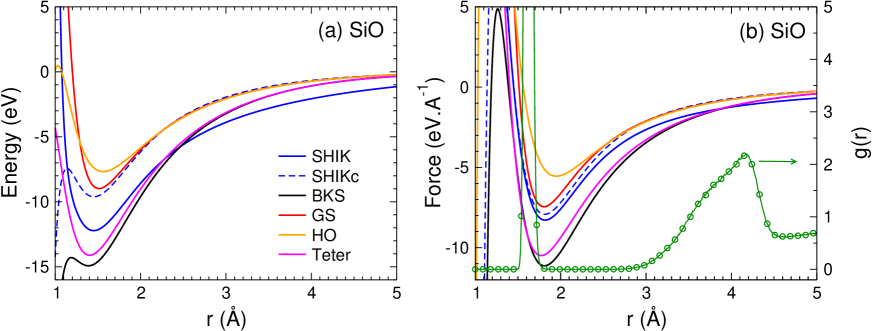
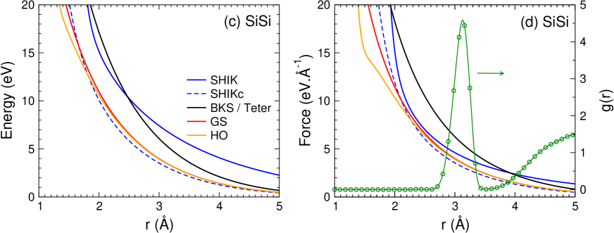
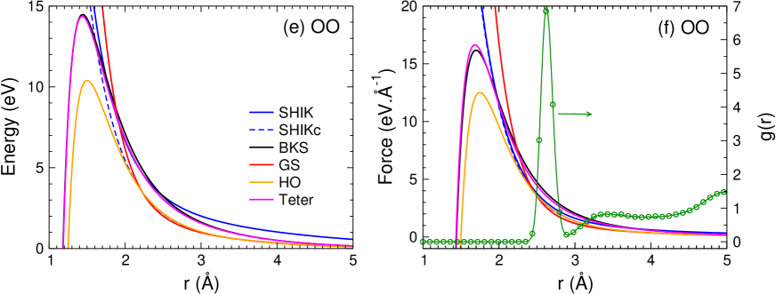
Figure 1: Distance dependence of the various interaction potentials [panels a), c), and e)] and their corresponding forces [panels b), d), and f)] for the SiO, SiSi and OO pairs. Also included in the latter panels are the corresponding pair correlation function as predicted by the SHIK potential at 300 K (symbols).

In Fig. 1 we plot the potential energy and the forces for the potentials considered. These graphs demonstrate that the different potentials and forces depend strongly on the chosen set of parameters which gives thus a first indication that the predicted glass properties will depend on the potential used. Note that, in order to show that we are indeed plotting the relevant range in distance, we also include the radial distribution function $g_{\alpha\beta}(r)$, with $\alpha,\beta\in\{{\rm Si,O}\}$ (green lines with symbols) in the graphs for the force. (These $g_{\alpha\beta}(r)$ are for the SHIK potential, at 300 K, but the other potentials predict radial distribution functions that are very similar.)

2.2 Simulation procedure

The systems we consider are pure silica and a sodium silicate with composition Na₂O-3SiO₂ corresponding to a Na₂O molar concentration of 25 %. The glass samples were produced by using the conventional melt-quench method. We used cubic boxes (periodic boundary conditions) that contained between 5000 and 600,000 particles, which corresponds to sizes between 4 and 20 nm at room temperature. For the long-range Coulomb interaction, the Wolf truncation method (see Eq. (2)) was employed when using the SHIK potential while for the other potentials this interaction was evaluated with the particle-particle particle-mesh (PPPM) solver algorithm with an accuracy of $5\times 10^{-5}$. As mentioned above, we also carried out simulations for silica using the SHIK parameters for the short-range part of the potential, and Coulomb interactions evaluated using PPPM algorithm, and the corresponding data will be labeled SHIKc.

The samples were first equilibrated at a high temperature in the canonical ensemble ($NVT$) using a fixed volume that corresponds to the experimental value of the density of the glass at room temperature [25]. These $NVT$ runs were done at 3600 K for silica and 3000 K for NS3, both for about 300 ps, a time that is sufficiently long to equilibrate the samples completely. These liquids were subsequently equilibrated in the $NPT$ ensemble (constant number of atoms, pressure, and temperature) at the same temperatures and at zero pressure. The lengths of these $NPT$ runs depended on the potential considered and were sufficiently long to equilibrate the samples, i.e. the mean squared displacement of the particles was more than 100 Å² (see below). For the GS potential, the $NPT$ equilibration of the NS3 liquid was done at 2100 K since for higher temperatures the samples became unstable because they were above the boiling point of the GS potential.

All simulations were carried out using the LAMMPS software [26] with a time step of 1.6 fs and using a Nosé-Hoover thermostat and barostat [27, 28, 29]. After equilibration, the liquid samples were quenched to 300 K in the $NPT$ ensemble at zero pressure. The cooling rate was 0.25 K/ps, i.e. a value that is relatively small for MD simulations of sodium silicate glasses with a comparable system size. Previous simulation studies have shown that this cooling rate is small enough so that the properties of the system do not depend on the cooling rate in a significant manner [19, 30, 31]. The glass samples at 300 K were then annealed in the $NPT$ ensemble for 160 ps before we started the mechanical tests. Since room temperature is well below the glass transition temperature, there is no need to consider a longer thermalization run as the atomic configurations are practically frozen, and neither the density nor the structural properties change noticeably.

The results presented in the following sections have been obtained by using for each potential only one sample per composition. For the structural and dynamical properties discussed in Sec. 3.1, the samples contained 36,480 and 38,400 atoms for SiO₂ and NS3, respectively, corresponding to box sizes around 8 nm. These system sizes are sufficiently large to make sample-to-sample fluctuations small.

For a given composition and a given potential, the mechanical properties presented in Subsec. 3.2 are the average obtained from one sample put under uniaxial tensile strain in the three independent directions, i.e. $x$, $y$, and $z$ directions, and the error bars correspond to standard deviation. To calculate the stress-strain curve we increased the dimension of the box in one direction linearly in time, $L(t)$. The strain is then given by

$$\epsilon(t)=\dot{\epsilon}t$$ (3)

where $\dot{\epsilon}$ is the strain rate. The stress tensor is obtained from the usual expression [32]

$${\bm{\sigma}}=\frac{1}{V}\sum_{i=1}^{N}\left[m_{i}\mathbf{v}_{i}\otimes\mathbf{v}_{i}+\mathbf{r}_{i}\otimes\mathbf{f}_{i}\right]$$ (4)

where $V$ and $N$ are the volume and the total number of atoms of the simulation box, respectively, while $m_{i}$ is the mass of atom $i$, and $\mathbf{v}_{i}$, $\mathbf{r}_{i}$ and $\mathbf{f}_{i}$ are the velocity, position and force vector of atom $i$, respectively.

3 Results

3.1 Structural and dynamical properties in the liquid and glassy states

The results in the present subsection are all for a cubic system with the size of the edge given by $L=8$ nm which corresponds to $N=36480$ and $N=38400$ atoms for SiO₂ and NS3, respectively. This size is sufficiently large to avoid that dynamic and static quantities are affected by finite size effects.

To investigate the dependence of the dynamics on the potential we have calculated the mean squared displacement (MSD) of a tagged particle:

$$r_{\alpha}^{2}(t)=\frac{1}{N_{\alpha}}\sum_{j=1}^{N_{\alpha}}\langle|{\bf r}_{j}(t)-{\bf r}_{j}(0)|^{2}\rangle\quad,$$ (5)

where $\alpha\in\{{\rm Si,O,Na}\}$ and $N_{\alpha}$ is the number of particles of species $\alpha$.

In Fig. 2 we show the time dependence of the MSD for Si, i.e., the species that moves the slowest. The temperatures are those at which we have equilibrated the samples in the $NPT$ ensemble and the curves correspond to the different potentials. One sees that, at these $T$s, the dynamics is already somewhat glassy in that at intermediate times the MSD has a plateau [33]. These graphs also show that at long times the MSD is a linear function of time, i.e., that the particles have reached the diffusive regime, indicating that the system is equilibrated.

In agreement with previous results [9], we find that the MSD at long times, and hence the diffusion constant, shows a very strong dependence on the potential, more than a factor of ten, although the structure of the glass does not vary that much (see below). Since it can be expected that the activation energy for the diffusion constant also depends on the potential considered, the diffusion constant at lower temperatures will differ even more, as previously reported in Ref. [9].

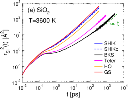
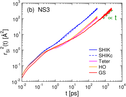
Figure 2: Mean squared displacement for silicon in the silica (a) and the NS3 (b) samples during the $NPT$ equilibration at high temperatures and at zero pressure. The different curves correspond to the potentials used and the dashed line shows the diffusive behavior. For SiO₂ the temperature is 3600 K. For NS3 the temperature is 3000 K except for the GS curve which is for 2100 K.

In Fig. 3 we show the temperature dependence of the mass density as predicted by the various potentials. These curves were obtained by cooling the samples at zero pressure from high temperatures to 0 K, i.e. at high $T$ they correspond to the equilibrium density of the system whereas at low $T$ to the density of the glass phase. The data demonstrates that the $T-$dependence of the density depends significantly on the potential: Not only the absolute values differ but also the slopes, i.e. the thermal expansion coefficients. For NS3 these slopes are larger than the ones for SiO₂ a result that matches the experimental findings [25]. Also included in the graphs are the experimental values of the density at room temperature (left most green diamond) and higher. For SiO₂, one sees that three potentials, namely Teter, HO, and GS, predict a density that is significantly too high, whereas the BKS and SHIK potentials are able to predict this quantity quite well. For NS3, the HO and SHIK potentials make an accurate prediction of the experimental density (green diamonds) whereas the ones by Teter and GS predict values that differ somewhat more from the experimental one. These graphs show thus that there are potentials which are able to give a quantitative good prediction of the density at room temperature. Note that the densities at room temperature are influenced by the cooling rate of the sample [19]. However, this dependence is relatively mild since the density is directly related to the fictive temperature at which the sample falls out of equilibrium and this temperature depends only logarithmically on the cooling rate. Thus if the discrepancy between the predicted density and the experimental value is too large, this cannot be rationalized by a too high cooling rate but must instead be considered as a flaw of the used potential.

We have also included in Fig. 3 the experimental values of the density at higher temperatures, calculated using the experimental values of the thermal expansion coefficient [25]. One recognizes that, for silica, the slope of this data matches very well the one predicted by the SHIK and BKS potentials while the three other potentials predict a larger expansion coefficient. For NS3 the graph shows that the HO potential predicts a slope which is in excellent agreement with the experimental data, the SHIK and Teter potentials are in fair agreement, while the GS potential is far off from the reality.

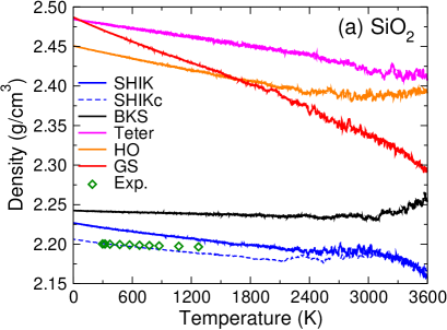
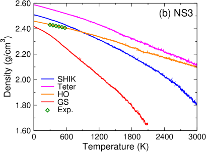
Figure 3: Temperature dependence of the density during the quench at zero pressure for silica and NS3, panels (a) and (b), respectively.

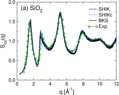
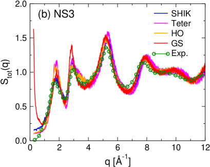
Figure 4: Structure factor as seen in neutron scattering experiments for silica (a) and NS3 (b) glasses at 300 K. Experimental data for silica are taken from Ref. [34] and for NS3 from Ref. [35].

We now probe how the properties of the glass depend on the potential. To start we show in Fig. 4 the static structure factor as seen in a neutron scattering experiment which is the weighted sum of the partial structure factors [33]:

$$S_{\rm tot}(q)=\frac{N}{\sum_{\alpha=\mathrm{Si,O,Na}}N_{\alpha}b_{\alpha}^{2}}\sum_{\alpha,\beta=\mathrm{Si,O,Na}}b_{\alpha}b_{\beta}S_{\alpha\beta}(q)\quad.$$ (6)

Here $q$ is the wave-vector, $b_{\alpha}$ is the neutron scattering length for species $\alpha$ and $S_{\alpha\beta}(q)$ is the partial structure factor: $\displaystyle S_{\alpha\beta}(q)=\frac{f_{\alpha\beta}}{N}\sum_{j=1}^{N_{\alpha}}\sum_{k=1}^{N_{\beta}}\left\langle\exp(i{\bf q}.({\bf r}_{j}-{\bf r}_{k}))\right\rangle$, $\alpha,\,\beta={\mathrm{Si,O,Na}}$, with f${}_{\alpha\beta}=1$ for ${\rm\alpha=\beta}$ and f${}_{\alpha\beta}=1/2$ otherwise, and $N$ the total number of atoms. From the figure we recognize that for the case of silica all considered potentials agree very well with the experimental data. This is not that surprising since in most cases the parameters of these potentials have been optimized to reproduce the structure of the glass. Qualitatively the same conclusion can be drawn for the case of NS3, panel (b). There is, however, one exception: The GS potential shows a strong increase of the signal at small $q$. This behavior indicates the presence of a phase separation, in this case the formation of large domains of Na atoms, and a visual inspection of the sample shows that this is indeed the case. (We note that this defect of the potential is not readily seen in the radial distribution functions and seems to have gone unnoticed so far.)

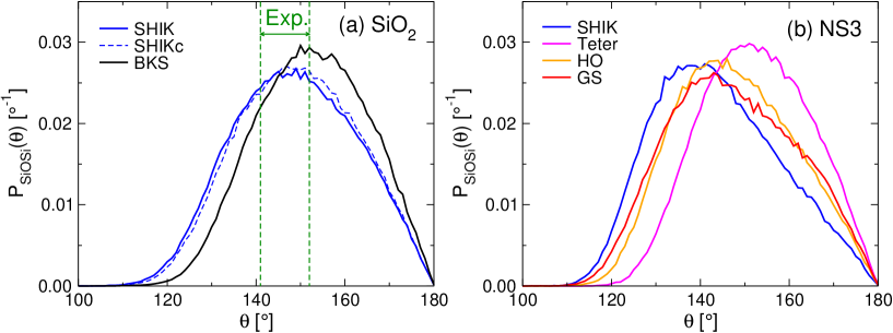
Figure 5: SiOSi angle distribution for silica (a) and NS3 (b) glasses at 300 K. The vertical green lines indicate the range of most probable SiOSi angle extracted from experimental studies (see Ref. [36]).

A further useful quantity to characterize the structure of silicate glasses is the distribution of the bond angles. Of particular interest is the angle SiOSi since it gives information about the relative orientation of two neighboring tetrahedra. For the case of SiO₂ this distribution is presented in Fig. 5a and we recognize that there is not much dependence on the potential considered and that all of them predict a position of the maximum of the distribution that is compatible with the experimental estimate for that angle [36]. Also for NS3 the distribution of this angle is basically independent of the potential used, Fig. 5b. The only exception is the data obtained from the Teter potential which predicts a peak at significantly larger angles. The calculated mean SiOSi angles are 143.7^∘, 147.7^∘, 147.1^∘ and 147.7^∘, and 152.3^∘ for the SHIK, GS, HO and Teter potential, respectively. When compared to the experimental mean value of 141.7^∘ extracted from ²⁹Si MAS NMR measurements [37], the SHIK data is in good agreement, while GS and HO present a reasonable one. In addition, one can compare these distributions with the ones from ab initio simulations [38, 39] of very similar compositions, which predicted peak positions close to 140^∘, i.e. values that are compatible with the one predicted by the SHIK, HO, and GS potentials, but not with the prediction by the Teter potential.

Finally we discuss two local structural quantities that probe the local environment of an atom, namely the oxygen speciation and the distribution of the $Q_{n}$ tetrahedral species in NS3. For the former we have used the first minimum in the radial distribution function of the Si-O pair to determine the connectivity of a given oxygen atom and thus to determine whether the atom is free (FO), non-bridging (NB), bridging (BO), or three-fold coordinated (TBO). In Fig. 6a we show the corresponding probability for the different potentials and one recognizes that the considered force fields all give the same distribution and it agrees very well with the experimental measurements [40]. Thus one can conclude that this quantity is very robust or in other terms the oxygen speciation is not very useful indicator for testing the quality of a potential. Things are different for the $Q_{n}$ species, i.e. the probability that a silicon atom is connected to exactly $n$ bridging oxygens, $n=0,1,2,3,4$. These probabilities are shown in Fig. 6b and one finds that, e.g., the frequency of the $Q_{3}$ structure depends significantly on the potential. In particular one observes that the GS potential gives a probability that is rather low with respect to the other potentials and also to the experimental data. Thus the observation that the fraction of $Q_{3}$ units depends significantly on the used potential indicates that this quantity can be used as an indicator for evaluating the quality of a potential. In addition we mention that the network depolymerization depends also on the cooling rate: For sodium silicate glasses, it has been shown that the percentage of $Q_{3}$ increases with decreasing quench rate while the $Q_{4}$ one is decreasing, and hence improve the agreement with the experimental data [31].

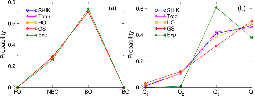
Figure 6: Distributions of oxygen speciations, panel (a), and $Q_{n}$ species, panel (b), for the NS3 glass at 300 K. The experimental data in panels (a) and (b) is from Ref. [40], and Ref. [41], respectively.

3.2 Mechanical properties of the glass

To determine the mechanical properties of the annealed glass samples we strained them in one direction using a strain rate of 0.5/ns. As we will show below this value is sufficiently small to obtain results that do not depend in a significant manner on the rate. We considered two ensembles for this transformation: A constant pressure ensemble ($NPT$) in which the pressures in the directions orthogonal to the strain were set to zero and a constant volume ensemble ($NVT$) in which the two orthogonal directions were not allowed to change, i.e. the cross section was constant. From this transformation we can thus directly obtain the stress-strain curve in the pulling direction discussed in the following.

3.2.1 System size and cooling rate dependence

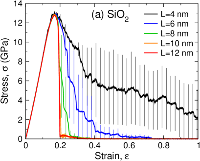
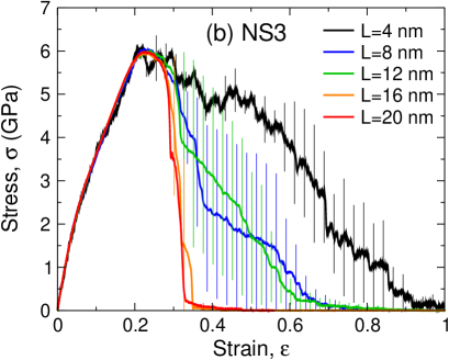
Figure 7: Dependence of stress-strain curve on the system size for the SHIK potential at 300 K. (a) Silica and (b) NS3. The system size ranges from around 5000 to around 600,000 atoms, corresponding to the increase of the size of the simulation box size from 4 nm to 20 nm at room temperature density (at zero strain). The error bars were estimated from the standard deviation for the three samples.

Before starting the discussion of the physical properties of the systems, we probe how these properties depend on the system size. Usually the properties of glasses can be obtained from simulations with relatively moderate system size, say $10^{3}-10^{4}$ atoms. However, elasticity and fracture are associated to non-local processes and hence finite size effects can be important. That this is indeed the case is demonstrated in Fig. 7 which shows the stress-strain curve for different (cubic) box sizes $L$. (These results are for the SHIK potential, but for the other force fields a similar behavior has been found [42].) Error bars have been estimated by considering three different samples. For the case of silica, panel (a), one finds that the elastic regime is basically independent of $L$. However, once the failure point (i.e. the strain at which the stress has a maximum) has been attained there are very strong finite size effects in that the small systems break in a much gentler manner than the large ones. Only if $L$ has reached 10 nm, which corresponds to around 75,000 atoms, the stress-strain curve becomes basically independent of the system size (see Refs. [43] and [44] for related studies).

For the case of NS3 the system size dependence is more pronounced in that one has to use systems of about $L=16$ nm, corresponding to about 300,000 atoms, before the stress-strain curve converges, see panel (b) in Fig. 7. These stronger finite size effects are likely related to the presence of the Na atoms which make a more heterogeneous structure in the NS3 glass compared to that of SiO₂ [45, 46]. However, for strains smaller than the failure point the curves for the different system sizes superimpose quite nicely and therefore also for this composition a system size with around 36,000 atoms, i.e. box size 8 nm, is sufficient to study the elastic regime.

In order to make a fair comparison of the behavior predicted by the different potentials we have used the same system size $L=8~{}$nm, which corresponds to $N=36480$ and $N=38400$ atoms for SiO₂ and NS3, respectively. Although for this system size one still can observe finite size effects, they are minor and hence do not preclude to understand which potentials give rise to a realistic fracture behavior and which ones do not.

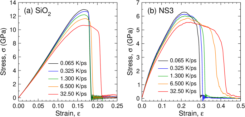
Figure 8: Stress-strain curves as predicted by the SHIK potential for glasses at 300 K, produced with different cooling rates. Panels (a) and (b) are for silica and NS3, respectively.

Another important parameter for the properties of a glass is the cooling rate with which the sample has been produced. In the past it has been found that structural quantities show a clear dependence on this cooling rate, often described by a logarithmic law [19, 30, 31] and hence one can expect that also the mechanical properties depend on this rate. In Fig. 8 we show that this is indeed the case in that with decreasing rate the failure strain decreases while the failure stress increases. At the same time a decreasing cooling rate leads to an increase of the slope in the elastic regime, i.e. the system becomes stiffer. Although these cooling rate effects are noticeable, we see that once the rate is below 0.3 K/s the effect is minor and hence the results discussed below, obtained with a rate of 0.25 K/s, are only mildly affected by the cooling rate used to produce the glass sample. (Note that the samples used in Fig. 8 were produced using the SHIK potential and by quenching firstly the liquids in the NVT ensemble to a temperature a bit below the glass transition, and then to 300 K in the NPT ensemble [42]. These samples contained 600,000 atoms.)

3.2.2 Fracture behavior and elastic moduli

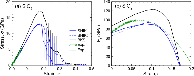
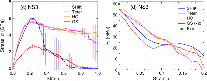
Figure 9: Mechanical responses of the glasses under uniaxial tension at 300 K. Panels (a) and (b) show the stress-strain curve and the tangent modulus for silica, respectively. The green symbols are the experimental data from Ref. [47]. The green dashed line in panel (b) is the polynomial fit from Ref. [48] to experimental data and its extrapolation to large strains. Panels (c) and (d): Same quantities as in panels (a) and (b) for the case of NS3.

We now discuss how the elastic moduli and the fracture behavior depend on the potential, the ensemble, and the way the Coulomb interaction is handled. In Fig. 9a we compare the stress-strain curves for BKS with the one for SHIK (obtained in the $NPT$ ensemble). One sees that the BKS glass is stiffer and stronger than the SHIK glass, and also breaks in a more ductile manner.

Also included in the graph is the data for the SHIKc potential with the full Coulomb interaction (blue dashed line). One sees that the results are very close to the SHIK curve (blue full line), i.e. when the Coulomb term is replaced by the expression given in Eq. (2), and hence one can conclude that Wolf truncation is a good approximation, a result which from the computational point of view is most advantageous. (Already for 38400 atoms one gains a factor of around 3 in CPU time.)

From the stress-strain curve one can obtain directly the tangent modulus which is defined as

$$E_{t}=\frac{d\sigma}{d\epsilon}\,,$$ (7)

where $\sigma$ is the stress in the pulling direction and $\epsilon$ the strain. This quantity is shown in Fig. 9b for the various potentials. In agreement with the curves from panel (a) we find that for all strains the BKS glass has a tangent modulus that is significantly larger than the one predicted by the SHIK potential. Interestingly, however, both potentials predict the same failure strain, i.e. $\epsilon_{f}\approx 0.17$, in excellent agreement with the experimental value of 0.18 [49]. For the SHIK potential we have also included the data as obtained by using the full Coulomb term and we see that the corresponding curve (dashed blue line) agrees very well with the one in which the Wolf term is used.

In addition, we have included in panels (a) and (b) of Fig. 9 the experimental data from Refs. [47] and [48]. One sees that these data sets agree very well with the predictions of the SHIK potential which is also able to reproduce accurately the Young’s modulus, i.e.

$$E=\lim_{\epsilon\to 0}E_{t}^{NPT}(\epsilon)\,,$$ (8)

with a value equal to 72 GPa, in very good agreement with the experimental value given by 73 GPa [25]. The prediction of the BKS potential is a bit less satisfactory, 86 GPa, in agreement with the findings from Ref. [43]. For the failure strength the BKS and SHIK potentials predict 17.6 GPa and 12.8 GPa, respectively, and the latter value is in excellent agreement with the experimental value of 12.6 GPa [49].

The stress-strain curve of NS3 as predicted by the different potentials is shown in Fig. 9c). Surprisingly we find that under $NPT$ conditions the HO and Teter potentials show no sign of fracture even if the sample is stretched to 100%. This shows that these potentials have a serious flaw in that they strongly overestimate the ductile behavior of NS3. Also the stress-strain curve from the GS potential is not realistic in that the stiffness in the elastic regime is strongly underestimated, the failure stress is too small, and that the fracture is way too ductile. Hence we conclude that these three potentials should not be used to study the fracture behavior of NS3. A much more reasonable stress-strain curves is found for the SHIK potential which shows a relatively brittle fracture. This brittleness is, however, less pronounced than the one found in SiO₂, see panel (a), in agreement with the expectation that the addition of Na will make the glass more ductile. The failure stress for the SHIK potential is around 6 GPa (see Table 2 for exact values), which compares reasonably well with the experimental values that are between 7.5 GPa and 11.7 GPa [50, 51] (this latter value is only an upper limit, see Ref. [50]).

The Young’s modulus of the NS3 glass, given by Eq. (8), is around 55 GPa for the SHIK, HO and Teter data (see Table 2 for exact values), in good agreement with the experimental value of 59.8 GPa [25], while the GS potential predicts a value of only 26 GPa, thus way too small. A more notable difference between the various potentials is found for the strain dependence of the tangent modulus, shown in Fig. 9d: While for the HO and Teter potentials, $E_{t}$ decreases basically in a linear manner, the SHIK and GS potentials show at intermediate strain a plateau before they decrease to zero. (Note that the data for the GS potential has been multiplied by a factor of 2.0 in order to bring it on the same scale as the other curves.) This plateau is also directly visible in the stress-strain curves in that they show at around $\epsilon=0.07$ a marked bend (see Fig. 9c). Elsewhere we will show that this rapid change in the effective stiffness of the sample is related to a change in the plastic behavior of the sample on the atomic scale [42].

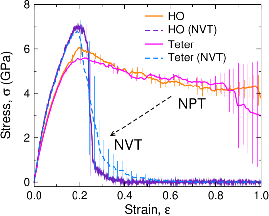
Figure 10: Influence of simulation ensemble on fracture at 300 K. The orange and magenta curves are the same as in Fig. 9c), i.e. $NPT$ ensemble. The violet and blue dashed curves are the data obtained in the $NVT$ ensemble.

The fact that neither the Teter nor the HO potential predict breaking if strained to 100% (see Fig. 9c), is astonishing since, from a structural point of view, these potentials give reasonable predictions. Thus one might wonder whether this unrealistic behavior is related to the ensemble used during the tensile loading. In Fig. 10 we thus show the stress-strain curve for the two potentials but now in the $NVT$ ensemble, i.e. the sample size orthogonal to the pulling direction is not allowed to change. We see that the so obtained stress-strain curves are completely different from the ones in the $NPT$ ensemble in that the formers indicate that the sample breaks in a rather brittle manner. A similar ensemble effect has also been observed for the case of silica [52]. Furthermore we note that in the elastic regime the curve becomes somewhat steeper, i.e. in the $NVT$ ensemble the system is stiffer than in the $NPT$ ensemble, and this change is also seen for the three other potentials, indicating that release of the constraint in the orthogonal directions decreases the tangent modulus, a result that certainly makes sense.

Finally we mention that, for the BKS as well as SHIK potential for silica, the fracture strain decreases significantly when one switches to the $NVT$ ensemble although the brittle nature of the fracture is independent of the ensemble. (Note that, as for NS3, the system is stiffer when working in the $NVT$ ensemble.) From these results we thus conclude that the choice of the ensemble is important, and thus the $NVT$ ensemble should be avoided for this type of measurements.

Quantity		E	C11	B	G	$\nu$	$\epsilon_{f}$	$\sigma_{f}$	$\rho$
Unit		GPa	GPa	GPa	GPa			GPa	g/cm3
Silica	SHIK	72.1	80.6	40.8	29.9	0.205	16.89	12.84	2.221
	SHIKc	65.0	76.0	40.9	26.3	0.235	17.31	13.01	2.200
	BKS	85.8	99.0	52.3	35.0	0.226	17.18	17.65	2.241
	Exp.	72.9a	78.0a	36.3a	31.3a	0.165a	18.00b	12.6b, 11-14c	2.201a
NS3	SHIK	55.7	66.2	36.4	22.4	0.245	22.43	6.05	2.472
	HO	54.8	68.1	39.3	21.6	0.268	19.99	6.05	2.433
	Teter	54.5	66.7	37.8	21.7	0.259	22.03	5.66	2.555
	GS	25.9	31.4	17.5	10.4	0.252	25.09	2.72	2.348
	Exp.	59.8a, 56d	69.5a	37.2a	24.3a, 22d	0.232a, 0.25d	20.85e	11.71e, 7.5f	2.431a

Table 2: Elastic constants (Young’s modulus $E$, longitudinal modulus $C_{11}$, bulk modulus $B$), Poisson’s ratio $\nu$, failure strain $\epsilon_{f}$ and stress $\sigma_{f}$ (GPa), and density $\rho$ at 300 K, compared with experimental data.
^a Ref. [25]
^b Ref. [49]
^c Ref. [53]
^d Ref. [54]
^e Ref. [50] (strength at 77 K, and the failure stress is overestimated, see discussion section in Ref. [50]).
^f Ref. [51] (strength at 77 K)

In the linear elastic regime one can characterize the mechanical behavior of the sample by the elastic constants given by the Young’s modulus from Eq. (8) and the longitudinal modulus given by

$$C_{11}=\lim_{\epsilon\to 0}E_{t}^{NVT}(\epsilon)\quad.$$ (9)

From $E$ and $C_{11}$ one can then obtain the bulk modulus $B$, the shear modulus $G$, and the Poisson’s ratio $\nu$ using the following relations [25, 55]:

$$E=\frac{9B(C_{11}-B)}{(3B+C_{11})}$$ (10)

$$G=\frac{3(C_{11}-B)}{4}$$ (11)

$$\nu=\frac{E}{2G}-1\quad.$$ (12)

The resulting values for the different potentials as well as the failure stress and failure strain are reported in Tab. 2. In this table we have also included the experimental values and one recognizes that overall the SHIK potential with the Wolf truncation is likely the most reliable potential. Note that this potential has the merit to be applicable not only to NS3 but, with the same set of parameters, also to SiO₂ and therefore also for compositions between the two systems [17].

4 Summary and Discussion

The goal of this work has been to investigate how the properties of the glasses, in particular their mechanical behavior, depend on the details of the interaction potential used to simulate the system, and to also to study the influence of the ensemble in which the simulations are done. In agreement with previous studies we have found that the structural quantities show a relatively mild dependence on the interaction potentials, with a notable exception for the GS potential that predicts a phase separation into sodium rich/poor regions. The temperature dependence of the density as well as the distribution of the different silicon species show instead a noticeable dependence on the potential and hence these quantities are more sensitive indicators for evaluating the quality of a potential.

A very strong dependence on the potential is found for the fracture behavior of the sample: While the Teter and HO potentials predict a plastic deformation at constant pressure even if the strain is 100%, the samples generated by the GS and SHIK potentials fail at a much smaller strain. Therefore the two former potentials should not be used for this type of studies. In addition, we have found that both structural and mechanical properties are not realistic when using the GS potential. If the sample is kept at constant geometry in the directions orthogonal to the pulling directions all potentials predict a brittle fracture.

Our results demonstrate that certain structural quantities show a dependence on the potential, but that the properties of the fracture show a much stronger one. The latter dependence is, however, definitely weaker than the ones found for dynamical quantities (see Ref. [9], for example). This can be understood from the fact that static properties depend mainly on the position of the particles close to the local minimum of the potential energy, while fracture and dynamic properties depend also on the position and height of the saddle points connecting these minima. Since for many systems there is only very limited experimental information about dynamic quantities, while elastic and inelastic measurements are much more abundant in the literature, the mechanical properties are thus a very attractive way to probe whether or not a potential is reliable.

A further important result of our study is the dependence of the fracture behavior on the system size. As in previous studies we have found that the structural quantities do depend only in a mild manner on the size of the system. In contrast to this, our study suggests that a reliable description of the fracture behavior can only be obtained for systems that have more than 75,000 particles, i.e. a box size of the order 10 nm for the case of silica and $L=16$ nm (300,000 atoms) for NS3. For smaller sizes, the elastic regime shows almost no dependence on the system size, while this dependence becomes very strong after the failure point and the system will present a fracture behavior that is much more ductile than a sufficiently large system.

Finally we have also documented the fact that the fracture behavior of the glass samples can show a strong dependence on the nature of the boundary conditions. If the traction is done under constant cross section condition, the samples will break in a brittle manner. However, if one fixes the pressure, as it is the case as in an experimental set-up, some potentials predict a much more ductile fracture or even no fracture at all up to a strain of 100%. This shows that for this type of studies one should use the $NPT$ ensemble and a potential that gives a realistic fracture behavior.

References

- 1. W. Kob. Computer simulations of supercooled liquids and glasses. J. Phys. Condens. Matter, 11:R85, 1999.
- 2. C. Massobrio, J. Du, M. Bernasconi, and P.S. Salmon. Molecular dynamics simulations of disordered materials, volume 215. Springer, 2015.
- 3. W. Kob and S. Ispas. First-principles simulations of glass-formers. arXiv:1604.07959 [cond-mat], 2016.
- 4. D. Marx and J. Hutter. Ab initio molecular dynamics: basic theory and advanced methods. Cambridge University Press, 2009.
- 5. S. Sundararaman, L. Huang, S. Ispas, and W. Kob. New optimization scheme to obtain interaction potentials for oxide glasses. J. Chem. Phys., 148:194504, 2018.
- 6. J. Behler. Perspective: Machine learning potentials for atomistic simulations. J. Chem. Phys., 145:170901, 2016.
- 7. H. Liu, Z. Fu, K. Yang, X. Xu, and M. Bauchy. Machine learning for glass science and engineering: A review. J. Non-Cryst. Solids, in press:119419, 2019.
- 8. M. Hemmatti and C.A. Angell. IR absorption of silicate glasses studied by ion dynamics computer simulation. I. IR spectra of SiO2 glass in the rigid ion model approximation. J. Non-Cryst. Solids, 217:236–249, 1997.
- 9. M. Hemmatti and C. A. Angell. Comparison of pair potential models for the simulation of liquid SiO2: Thermodynamic, angular-distribution, and diffusional properties. Physics Meets Mineralogy: Condensed Matter Physics in the Geosciences, pages 325–339, 2000.
- 10. T.F. Soules, G.H. Gilmer, M.J. Matthews, J.S. Stolken, and M.D. Feit. Silica molecular dynamic force fields - A practical assessment. J. Non-Cryst. Solids, 357:1564–1573, 2011.
- 11. B.J. Cowen and M.S. El-Genk. On force fields for molecular dynamics simulations of crystalline silica. Comput. Mater. Sci., 107:88–101, 2015.
- 12. X. Yuan and A.N. Cormack. Local structures of MD-modeled vitreous silica and sodium silicate glasses. J. Non-Cryst. Solids, 283:69–87, 2001.
- 13. M. Bauchy. Structural, vibrational, and elastic properties of a calcium aluminosilicate glass from molecular dynamics simulations: The role of the potential. J. Chem. Phys., 141:024507, 2014.
- 14. J. Habasaki and I. Okada. Molecular dynamics simulation of alkali silicates based on the quantum mechanical potential surfaces. Mol. Simul., 9:319–326, 1992.
- 15. A. N. Cormack, J. Du, and T. R. Zeitler. Alkali ion migration mechanisms in silicate glasses probed by molecular dynamics simulations. Phys. Chem. Chem. Phys., 4:3193–3197, 2002.
- 16. B. Guillot and N. Sator. A computer simulation study of natural silicate melts. Part I: Low pressure properties. Geochim. Cosmochim. Acta, 71:1249–1265, 2007.
- 17. S. Sundararaman, L. Huang, S. Ispas, and W. Kob. New interaction potentials for alkali and alkaline-earth aluminosilicate glasses. J. Chem. Phys., 150:154505, 2019.
- 18. B.W.H. van Beest, G.J. Kramer, and R.A. van Santen. Force fields for silicas and aluminophosphates based on ab initio calculations. Phys. Rev. Lett., 64:1955, 1990.
- 19. K. Vollmayr, W. Kob, and K. Binder. Cooling-rate effects in amorphous silica: A computer-simulation study. Phys. Rev. B, 54:15808–15827, 1996.
- 20. J. Horbach and W. Kob. Static and dynamic properties of a viscous silica melt. Phys. Rev. B, 60:3169, 1999.
- 21. J. Luo, Y. Zhou, S.T. Milner, C.G. Pantano, and S.H. Kim. Molecular dynamics study of correlations between IR peak position and bond parameters of silica and silicate glasses: Effects of temperature and stress. J. Am. Ceram. Soc., 101:178–188, 2018.
- 22. M.P. Allen and D.J. Tildesley. Computer simulation of liquids. Oxford University Press, 2017.
- 23. D. Wolf, P. Keblinski, S. R. Phillpot, and J. Eggebrecht. Exact method for the simulation of Coulombic systems by spherically truncated, pairwise summation. J. Chem. Phys., 110(17):8254–8282, May 1999.
- 24. A. Carré, L. Berthier, J. Horbach, S. Ispas, and W. Kob. Amorphous silica modeled with truncated and screened Coulomb interactions: A molecular dynamics simulation study. J. Chem. Phys., 127:114512, 2007.
- 25. N.P. Bansal and R.H. Doremus. Handbook of glass properties. Academic Press, Orlando, 1986.
- 26. S. Plimpton. Fast parallel algorithms for short-range molecular dynamics. J. Comput. Phys., 117:1–19, 1995.
- 27. S. Nosé. A unified formulation of the constant temperature molecular dynamics methods. J. Chem. Phys., 81:511–519, 1984.
- 28. W.G. Hoover. Canonical dynamics: Equilibrium phase-space distributions. Phys. Rev. A, 31:1695–1697, 1985.
- 29. W.G. Hoover. Constant-pressure equations of motion. Phys. Rev. A, 34:2499–2500, 1986.
- 30. J.M.D. Lane. Cooling rate and stress relaxation in silica melts and glasses via microsecond molecular dynamics. Phys. Rev. E, 92:012320, 2015.
- 31. X. Li, W. Song, K. Yang, N.A. Krishnan, B. Wang, M.M. Smedskjaer, J.C. Mauro, G. Sant, M. Balonis, and M. Bauchy. Cooling rate effects in sodium silicate glasses: Bridging the gap between molecular dynamics simulations and experiments. J. Chem. Phys., 147:074501, 2017.
- 32. A.P. Thompson, S. Plimpton, and W. Mattson. General formulation of pressure and stress tensor for arbitrary many-body interaction potentials under periodic boundary conditions. J. Chem. Phys., 131:154107, 2009.
- 33. K. Binder and W. Kob. Glassy materials and disordered solids: An introduction to their statistical mechanics. World Scientific, Singapore, 2011.
- 34. S. Susman, K.J. Volin, D.G. Montague, and D.L. Price. Temperature dependence of the first sharp diffraction peak in vitreous silica. Phys. Rev. B, 43:11076–11081, 1991.
- 35. M. Pöhlmann. Structure and dynamics of hydrous silica(tes) as seen by molecular dynamics computer simulations and neutron scattering. PhD thesis, Technische Universität München and Université Montpellier 2, 2005.
- 36. W.J. Malfait, W.E. Halter, and R. Verel. 29Si NMR spectroscopy of silica glass: T1 relaxation and constraints on the Si–O–Si bond angle distribution. Chem. Geol., 256:269–277, 2008.
- 37. F. Angeli, O. Villain, S. Schuller, S. Ispas, and T. Charpentier. Insight into sodium silicate glass structural organization by multinuclear NMR combined with first-principles calculations. Geochimica et Cosmochimica Acta, 75:2453–2469, 2011.
- 38. D. Kilymis, S. Ispas, B. Hehlen, S. Peuget, and J.-M. Delaye. Vibrational properties of sodosilicate glasses from first-principles calculations. Phys. Rev. B, 99:054209, 2019.
- 39. A. Tilocca and N.H. de Leeuw. Structural and electronic properties of modified sodium and soda-lime silicate glasses by Car-Parrinello molecular dynamics. J. Mater. Chem., 16:1950–1955, 2006.
- 40. H.W. Nesbitt, G.M. Bancroft, G.S. Henderson, R. Ho, K.N. Dalby, Y. Huang, and Z. Yan. Bridging, non-bridging and free (O2) oxygen in Na2O-SiO2 glasses: An X-ray Photoelectron Spectroscopic (XPS) and Nuclear Magnetic Resonance (NMR) study. J. Non-Cryst. Solids, 357:170–180, 2011.
- 41. H. Maekawa, T. Maekawa, K. Kawamura, and T. Yokokawa. The structural groups of alkali silicate glasses determined from 29Si MAS-NMR. J. Non-Cryst. Solids, 127:53–64, 1991.
- 42. Z. Zhang. Fracture of oxide glasses: New insights from atomistic simulations. PhD Thesis, University of Montpellier, 2020.
- 43. F. Yuan and L. Huang. Molecular dynamics simulation of amorphous silica under uniaxial tension: From bulk to nanowire. J. Non-Cryst. Solids, 358:3481–3487, 2012.
- 44. A. Pedone, M.C. Menziani, and A.N. Cormack. Dynamics of Fracture in Silica and Soda-Silicate Glasses: From Bulk Materials to Nanowires. J. Phys. Chem. C, 119:25499–25507, 2015.
- 45. G. N. Greaves. EXAFS and the structure of glass. J. Non-Cryst. Solids, 71:203, 1985.
- 46. J. Horbach, W. Kob, and Binder K. Dynamics of sodium in sodium disilicate: Channel relaxation and sodium diffusion. Phys. Rev. Lett., 88:125502, 2002.
- 47. J.T. Krause, L. R. Testardi, and R. N. Thurston. Deviations from linearity in the dependence of elongation on force for fibers of simple glass formers and of glass optical lightguides. Phys. Chem. Glass., 20:135–9, 1979.
- 48. P.K. Gupta and C.R. Kurkjian. Intrinsic failure and non-linear elastic behavior of glasses. J. Non-Cryst. Solids, 351:2324–2328, 2005.
- 49. W. Griffioen. Optical fiber mechanical reliability. Eindhoven University of Technology, 1995.
- 50. N.P. Lower, R.K. Brow, and C.R. Kurkjian. Inert failure strain studies of sodium silicate glass fibers. J. Non-Cryst. Solids, 349:168–172, 2004.
- 51. C.R. Kurkjian and P.K. Gupta. Intrinsic strength and the structure of glass. In Proc. Int. Congr. Glass, volume 1, pages 11–18, 2001.
- 52. A. Pedone, G. Malavasi, M.C. Menziani, U. Segre, and A.N. Cormack. Molecular Dynamics Studies of Stress-Strain Behavior of Silica Glass under a Tensile Load. Chem. Mater., 20:4356–4366, 2008.
- 53. W. A. Smith and T. M. Michalske. DOE contract# DE‐AC04‐0dpoo789, 1990.
- 54. K. Januchta, T. To, M.S. Bødker, T. Rouxel, and M.M. Smedskjaer. Elasticity, hardness, and fracture toughness of sodium aluminoborosilicate glasses. J. Am. Ceram. Soc., 102:4520–4537, 2019.
- 55. Q. Zhao, M. Guerette, G. Scannell, and L. Huang. In-situ high temperature Raman and Brillouin light scattering studies of sodium silicate glasses. J. Non-Cryst. Solids, 358:3418–3426, 2012.