Topological elasticity of non-orientable ribbons

Abstract

In this article, we unravel an intimate relationship between two seemingly unrelated concepts: elasticity, that defines the local relations between stress and strain of deformable bodies, and topology that classifies their global shape. Focusing on Möbius strips, we establish that the elastic response of surfaces with non-orientable topology is: non-additive, non-reciprocal and contingent on stress-history. Investigating the elastic instabilities of non-orientable ribbons, we then challenge the very concept of bulk-boundary-correspondence of topological phases. We establish a quantitative connection between the modes found at the interface between inequivalent topological insulators and solitonic bending excitations that freely propagate through the bulk non-orientable ribbons. Beyond the specifics of mechanics, we argue that non-orientability offers a versatile platform to tailor the response of systems as diverse as liquid crystals, photonic and electronic matter.

I Introduction

Sewing the first piece of fabric, prehistoric men laid out the first principles of metamaterial design Kvavadze et al. (2009): elementary units assembled into geometrical patterns form structures with mechanical properties that can surpass those of their constituents Bertoldi et al. (2017). In the early 2010’s, building on quantitative analogies with the topological phases of quantum matter, researchers laid out robust design rules for metamaterials supporting mechanical deformations immune from geometrical and material imperfections  Kane and Lubensky (2014); Prodan and Prodan (2009); Süsstrunk and Huber (2015); Nash et al. (2015); Huber (2016); Bertoldi et al. (2017); Mao and Lubensky (2018). Today, mechanical analogs of virtually all topological phases of electronic matter have been experimentally realized, or theoretically designed, with mechanical components as simple as coupled gyroscopes or lego pegs Nash et al. (2015); Süsstrunk and Huber (2015); Chen et al. (2014); Bertoldi et al. (2017); Barlas and Prodan (2018); Süsstrunk and Huber (2016); Mitchell et al. (2018). The basic strategy consists in connecting mechanical systems with gapped vibrational spectra having topologically distinct eigenspaces Hasan and Kane (2010); Bernevig ; Mao and Lubensky (2018). At the interface, this mismatch causes a local gap closing revealed by linear edge modes topologically protected from disorder and backscattering. Until now, as topological mechanics was inspired by analogies with condensed matter, it has been essentially restrained to metamaterials assembled from repeated mechanical units, that inherit robustness from the topology of their abstract vibrational eigenspace Mao and Lubensky (2018); Sun2019 .

In this article, we elucidate the consequences of real-space topology on the mechanics of homogeneous materials. Firstly, we demonstrate that non-orientability makes Möbius strips’ elasticity: non-additive, nonreciprocal and multistable. In particular, we demonstrate how the static deformations of non-orientable surfaces encode their stress history: Möbius strips have a mechanical memory. Secondly, we address the impact of non-orientability on the paradigmatic Euler elastic instability. We show that the associated buckling patterns propagate as solitary waves on Möbius strips. We finally establish the equivalence between these non-linear bulk excitations and the edge modes found at the interface between inequivalent topological states in one-dimensional topological insulators Hasan and Kane (2010).

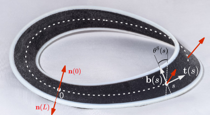
Figure 1: A non-orientable elastic ribbon. Example of a 3D printed Möbius strip of width $1\,\rm cm$. The dotted white line indicates the base circle $\mathbf{C}(s)$. The shear angle $\theta^{\rm s}$ is defined with respect to the local normal to the surface $\mathbf{n}(s)$ (red arrows). Note that $\mathbf{n}(s)$ reverses its sign after one full turn around the strip $\mathbf{n}(0)=-\mathbf{n}(L)$. The tangent, $\mathbf{t}(s)$, and bi-normal, $\mathbf{b}(s)$, vectors are indicated with white arrows.

II Topological elasticity of non-orientable surfaces

Simply put, a non-orientable surface is a one-sided thin sheet. A paradigmatic example is given by the Möbius strip shown in Fig. 1 that can be easily replicated by applying a half twist to a band of paper before glueing its two ends. Orientability is indeed a global (topological) property that can be altered only by cutting and gluing back a geometrical surface. In contrast, linear elasticity describes local deformations in response to gentle mechanical stresses. Before introducing a technical framework to relate these two seemingly unrelated concepts, let first us gain some intuition about their relationship. We consider the simple example of a Möbius strip made of an elastic material showed in Fig. 1. The shear deformations of the strip is locally quantified by the angle $\theta^{\rm S}(s)$, where $s\in[0,L]$ indicates the curvilinear coordinates along the strip centerline. $\theta^{\rm S}(s)$ is a rotation angle defined with respect to the vector $\mathbf{n}(s)$ normal to the surface. A direct consequence of non-orientability is that no stress distribution can yield homogeneous shear deformations over a Möbius strip. As illustrated in Fig. 1, when transported around the entire strip, $\mathbf{n}(s)$ changes sign, thereby implying that $\theta^{\rm S}(0)=-\theta^{\rm S}(L)$, and that the shear angle must vanish at least once along the ribbon. The impossibility to assign an unambiguous orientation to the surface constrains the ribbon to remain undeformed at one point whatever the magnitude of the applied stress. We now account for this topological protection against shear by describing the elasticity of non-orientable ribbons as a $\mathbb{Z}_{2}$ gauge theory.

II.1 Orientability as a $\mathbb{Z}_{2}$ gauge charge.

For sake of clarity, we restrain ourselves to strips of constant width $w$ akin to that showed in Figs. 1, and 2. They are defined as ruled surfaces ${\mathbf{S}}(s,z)={\mathbf{C}}(s)+z{\mathbf{b}}(s)$ where ${\mathbf{C}}(s)$ is a base circle of perimeter $L$, and $\mathbf{b}(s)$ is a unit-vector field normal to the tangent-vector field ${\mathbf{t}}(s)$, see Fig. 1. Given this definition $s\in[0,L]$ and $z\in[-w/2,w/2]$. We stress that the direction of $\mathbf{b}(s)$ is arbitrary: a local transformation $\mathbf{b}(s)\to\epsilon(s)\mathbf{b}(s)$, where $\epsilon(s)=\pm 1$ leaves the strip geometry unchanged. The tangent to the base circle $\mathbf{t}(s)$ being unambiguously defined, the normal vector ${\mathbf{n}}(s)=\mathbf{t}(s)\times\mathbf{b}(s)$ is defined up to the same $\epsilon(s)$ sign factor as $\mathbf{b}(s)$.

By definition, non-orientable strips correspond to shapes where the fields $\epsilon(s)\mathbf{b}(s)$ and $\epsilon(s)\mathbf{n}(s)$ are discontinuous regardless of the sign convention $\epsilon(s)$. This intrinsic ambiguity in defining the orientation of the (bi)normal vector is better illustrated when discretizing the strip, see Fig. 2. Setting $s=ia$, where $a=L/N$ and $i\in[1,N-1]$, we introduce the $\mathbb{Z}_{2}$ gauge field $\eta_{i,i+1}=\epsilon_{i}\epsilon_{i+1}$ which represents the connection between adjacent sign conventions. The topological charge ${\mathcal{O}}=\prod_{i=1}^{N}\eta_{i,i+1}$, defines the surface orientability: orientable surfaces correspond to $\mathcal{O}=+1$ and nonorientable ones to $\mathcal{O}=-1$. The independence of $\mathcal{O}$ with respect to the sign convention becomes clear when applying the series of gauge transformations sketched in Figs. 2a and  2b. Starting from an arbitrary position $i_{\rm G}+1$ and moving along the base circle, wherever a link with $\eta_{i,i+1}=-1$ is found, we change the sign of $\epsilon_{i+1}$. This transformation reverses simultaneously the signs of both $\eta_{i,i+1}$ and $\eta_{i+1,i+2}$ thereby leaving $\mathcal{O}$ unchanged. Moving along the strip and repeating this procedure, we find that the gauge field on all links but the last one can be set to $\eta=+1$. On the last link, it takes the value $\eta_{i_{\rm G},i_{\rm G}+1}=\mathcal{O}$. Therefore, when $\mathcal{O}=-1$ there is an obstruction to define a homogeneous surface orientation: the surface is non-orientable.

Figure 2: Orientability as a $\mathbb{Z}_{2}$ gauge charge. Two discretized ribbons: a Möbius strip (a.), and a cylinder (b.). The arrows indicate the orientation of the $\mathbf{b}_{i}$ vectors, and the plaquettes’ color the sign of $\eta_{i,i+1}$ on each link, yellow: $\eta_{i,i+1}=+1$, blue: $\eta_{i,i+1}=-1$. The gauge transformations described in Section II.1 are illustrated by the red arrows. a. No series of orientation-gauge transformations can result in a homogeneous $\eta$ field on a Möbis strip: $\mathcal{O}=-1$. (b.) Starting from a heterogeneous $\eta$ field, the gauge transforms result in a homogeneous $\eta=+1$ field on a orientable cylinder: $\mathcal{O}=+1$.

II.2 Elasticity of twisted elastic strips.

We now make use of this geometric framework to describe the elastic response of a soft Möbius strip having a stress-free equilibrium shape defined by the triad $(\mathbf{t}^{0}(s),\mathbf{b}^{0}(s),\mathbf{n}^{0}(s))$. For sake of simplicity, we do not resort to the full Foppl-von Karman theory of elastic plates Audoly and Pomeau (2010). Instead, we consider simplified models to single out the impact of non-orientability on shear, twist and bend deformations leaving a more realistic mechanical description for future work. The amplitude of the pure-shear, $\theta^{\rm S}(s)$, and pure-twist angles, $\theta^{\rm T}(s)$, are usually defined from the deformation vector $\mathbf{u}(s)=\mathbf{b}(s)-\mathbf{b}^{0}(s)\equiv\theta^{\rm S}(s)\mathbf{t}^{0}(s)+\theta^{\rm T}(s)\mathbf{n}^{0}(s)$. As discussed in the previous section, however, both $\mathbf{b}(s)$ and $\mathbf{n}(s)$ are defined up to a sign convention $\epsilon(s)$, while all physical quantities must be independent of this arbitrary choice. We therefore introduce the orientation-independent deformation field:

$$\left(\epsilon\mathbf{u}\right)=(\epsilon\theta^{\rm S})\mathbf{t}^{0}+\theta^{\rm T}(\epsilon\mathbf{n}^{0}).$$ (1)

$\left(\epsilon\mathbf{u}\right)$ is invariant upon the orientation transformation: $\{\epsilon(s)\to-\epsilon(s),\,\theta^{\rm S}(s)\to-\theta^{\rm S}(s),\,\theta^{\rm T}(s)\to\theta^{\rm T}(s)\}$. Due to the possibly discontinuous nature of the $\epsilon$ field, we first define the harmonic elasticity associated to $(\epsilon u)$ by resorting to a discretization of the ribbon geometry. The simplest harmonic elasticity is then given by ${\mathcal{E}}=K/(2a)\sum_{i}\left[(\epsilon\mathbf{u})_{i+1}-(\epsilon\mathbf{u})_{i}\right]^{2}$ where $K$ is an isotropic elastic constant, and $\mathcal{E}$ is readily recast into:

$${\mathcal{E}}=\frac{K}{2a}\sum_{i}\left[\mathbf{u}_{i+1}-\eta_{i,i+1}\mathbf{u}_{i}\right]^{2}.$$ (2)

The invariance of $(\epsilon_{i}u_{i})$ under orientation transformation translates into a $\mathbb{Z}_{2}$ gauge symmetry of the elastic energy: $\{\eta_{i,i\pm 1}\to-\eta_{i,i\pm 1},\,\theta^{\rm S}_{i}\to-\theta^{\rm S}_{i},\,\theta^{\rm T}_{i}\to\theta^{\rm T}_{i}\}$. Following the procedure sketched in Fig. 2, Eq. (2) can be simplified by gauging away the $\eta_{i,i+1}$ at all sites but one, at $i\equiv i_{\rm G}$ where $\eta_{i_{\rm G},i_{\rm G}+1}=\mathcal{O}$. For this gauge choice, $\mathcal{E}$ takes the compact form: ${\mathcal{E}}=\frac{K}{2a}\sum_{i}(\left[\theta^{\rm S}_{i+1}-\theta^{\rm S}_{i}\right]^{2}+\left[\theta^{\rm T}_{i+1}-\theta^{\rm T}_{i}\right]^{2})+\frac{K}{a}\left(1-{\mathcal{O}}\right)\theta^{\rm S}_{i_{\rm G}}\theta_{i_{\rm G}+1}^{\rm S}$, where we have implicitly assumed $w/L$ to be vanishingly small and left finite-size geometrical corrections to future work Kamien (2002). The last term of this expression accounts for the coupling between the topological charge $\mathcal{O}$ and the shear angle at the unspecified site $i_{\rm G}$. Continuum elasticity then follows from the limit $a\to 0$ in Eq. (2):

$${\mathcal{E}}(\{\theta^{\rm S},\theta^{\rm T}\})=\frac{K}{2}\int_{0}^{L}\!\!\left(\partial_{s}\theta^{\rm S}\right)^{2}+\left(\partial_{s}\theta^{\rm T}\right)^{2}{\rm d}s\\ +(1-\mathcal{O})\lim_{a\to 0}\frac{K}{a}\left[(\theta^{\rm S})^{2}+a\theta^{\rm S}\partial_{s}\theta^{\rm S}\right]_{s=s_{\rm G}}.$$ (3)

For orientable strips, one recovers the familiar harmonic energy of elastic bodies. In contrast, for Möbius strips where ${\mathcal{O}}=-1$, the topological term in Eq. (3) constrains the continuous shear deformations to vanish at $s=s_{\rm G}$ . Two comments are in order: Firstly, unlike shear deformations, we find that twist deformations are insensitive to orientability and obey uncronstrained harmonic elasticity. Secondly, we stress that the location of the zero-shear point $s_{\rm G}$ is an independent and crucial gauge degree of freedom that must be dealt with when computing the fluctuations and mechanical response of non-orientable elastic ribbons as illustrated below.

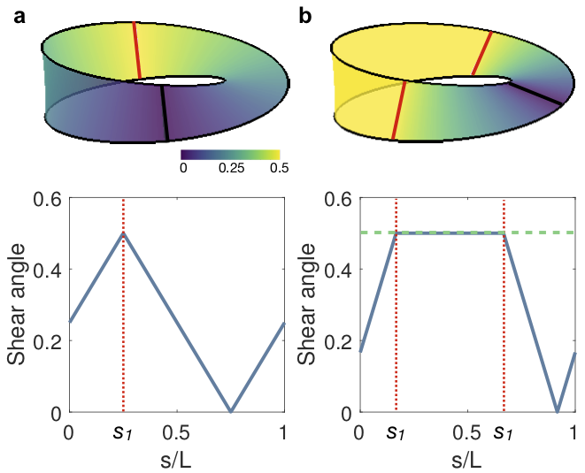
Figure 3: Nonlinear response to shear stress. Top panels: the color indicates the magnitude of the shear angle along the Möbius strips. The red lines show the positions of the applied stresses, and the dark line the position of $s_{\rm G}$. Bottom panels: corresponding plots of $\theta^{\rm S}(s)$. a. Response to a point-wise stress source $\sigma(s)=\sigma\delta(s-1/4)$ with $\sigma=K$. The shear angle decays linearly from the stress source and vanishes at $s=3/4$. b. Nonlinearity: Response to two point-wise stress sources $\sigma^{\rm S}=K[\delta(s-1/6)-\delta(s-(1/6+1/2))]$. The deformations computed from the minimization of the elastic energy as explained in Appendix A.3 vanish at $s_{\rm G}={11}/{12}$. The deformations computed from the minimization of the elastic energy (solid line) are markedly different from the linear supperposition of two responses to two individual point sources (dashed line).

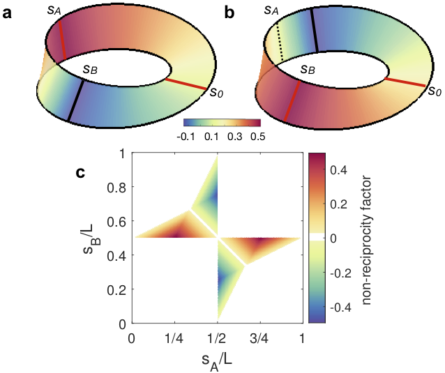
Figure 4: Nonreciprocal response to shear stress. A Möbius strip is sheared by a localized stress distribution $\sigma_{0}=\sigma\delta(s-s_{0})$ with $\sigma=K$ and $s_{0}=0$. a. Overall excess shear deformations $\theta_{A}(s)$ due to an additional stress $\sigma_{A}=\sigma\delta(s-s_{A})$ applied at $s_{A}=7/16$. b. Plot of the excess shear deformations $\theta_{B}(s)$ measured when $\sigma_{A}$ is released and $\sigma_{B}=\sigma\delta(s-s_{B})$ is applied at ($s_{B}=23/32$). Same color map as in a. Together the plots reveal that $\theta_{A}(s_{B})\neq\theta_{B}(s_{A})$. c Variations of the non-reciprocity factor $\Delta\theta$ as a function of the locations of $s_{A}$ and $s_{B}$. The finite value of $\Delta\theta$ over a finite region of space proves that the Maxwell-Betti theorem breaks down on non-orientable elastic surfaces: non-oreinatble elasticity is non-reciprocal.

Figure 5: Elastic Memory. a. Three different shear deformations are compatible with mechanical equilibrium when point-wise shear stresses of equal strength $K$ are applied at $s=1/6,\,1/2,$ and $5/6$. The colors indicate the magnitude of the shear deformations $\theta^{\rm S}$, same colormap as in Fig. 3. b. Corresponding time variations of the stress amplitude. c Spatial and temporal variations of the effective potential $U_{3}(s,t)$. The blue circle indicates the location of the instantaneous minimum of $U_{3}$ where $s_{\rm G}$ is trapped.

II.3 Non-additive elasticity

From now on the ribbon elasticity is prescribed by Eq. (3), and the constraint $\theta^{\rm S}(s_{\rm G})=0$. It then readily follows that non-orientable ribbons cannot support any homogeneous shear deformation as anticipated in the introduction of Section II and further discussed in Appendix A.1. The simplest mechanical stress we can consider is a pointwise shear localized at an arbitrary position $s_{1}$: $\sigma^{\rm S}(s)=\sigma\delta(s-s_{1})$. The resulting deformations shown in Fig. 3a are computed minimizing $\mathcal{E}+\mathcal{W}$ with respect to both the shear and gauge degrees of freedom, where $\mathcal{W}=-\int_{0}^{L}\sigma^{\rm S}(s)\theta^{\rm S}(s){\rm d}s$ is the work performed by the external stress, see Appendix A. We find a positive elastic response that vanishes at a single point located at maximal distance from the stress source:

$$\theta_{1}(s;s_{1}) =\frac{\sigma}{2K}\left|s-s_{1}-\operatorname{sgn}(s-s_{1})\frac{L}{2}\right|.$$ (4)

This simple expression has a deep consequence: the response of Möbius strips to shear stresses is intrinsically nonlinear, although the local stress-strain relation is linear. We establish this counter intuitive property by considering the case of two identical stress sources: $\sigma^{\rm S}(s)=\sigma\left[\delta(s-s_{1})+\delta(s-s_{2})\right]$. The linear superposition of two $\theta_{1}$ functions would result in strictly positive shear deformations over the whole strip which is topologically prohibited as $\theta^{\rm S}$ must vanish at least at one point $s_{\rm G}$. We therefore conclude that the response of Möbius strips to shear stresses is not pairwise additive and therefore nonlinear. This property is illustrated in Fig. 3b where we compare the shear angle $\theta_{2}(s;s_{1},s_{2})$ computed from the minimization of $\mathcal{E}+\mathcal{W}$ with respect to $\theta^{\rm S}$ and $s_{\rm G}$ to that that derived from a mere superposition principle, see also Appendix A.3.

We explain below the practical consequence of this topological frustration.

II.4 Non-reciprocal elasticity

The static response of elastic bodies is generically reciprocal. In virtue of the so-called Maxwell-Betti theorem, the deformations measured at a point $B$, as a result of a force applied at a point $A$, are identical to the deformations measured at point $A$ as a result of the same force when applied at point $B$ Maxwell (1864); Betti (1872); Coulais et al. (2017). The mechanics of non-orientable surfaces, however, is not reciprocal. To prove this counterintuitive results, we consider as a refence state a Möbius strip sheared by a localized source $\sigma_{0}=\sigma\delta(s-s_{0})$ causing a deformation $\theta_{1}(s;s_{0})$. Let us now apply an additional stress $\sigma$ at $s_{A}$, and measure the response at $s_{B}$: $\theta_{A}(s_{B})=\theta_{2}(s_{B};s_{0},s_{A})-\theta_{1}(s;s_{0})$. We now release the stress applied at $s_{A}$, apply as stress $\sigma$ at $s_{B}$, and measure the response at $s_{A}$: $\theta_{B}(s_{A})=\theta_{2}(s;s_{0},s_{B})-\theta_{1}(s;s_{0})$. The two corresponding excess shear angles are shown in Figs. 4a and 4b and are obviously different. Following Coulais et al. (2017), we plot in Fig. 4c the non-reciprocity factor $\Delta\theta=[\theta_{A}(s_{B})-\theta_{A}(s_{B})]K/\sigma$ as a function of the locations of the two applied stresses ($s_{A}$ and $s_{B}$). We find that $\Delta\theta$ is finite over a large fraction of the parameter space and extremal when the stress sources are distant from $L/4$ and $L/2$ from $s_{0}$: the mechanical response of the strip is non reciprocal. Two comments are in order. By contrast with the polar metamaterials considered in Coulais et al. (2017), here non-reciprocity does not rely on non-proportional response. The constitutive relation between stress and strain is linear, the strip is not unstable, and no floppy mode is excited. Non-reciprocity solely stems from the non-additive response of non-orientable strips. We also stress that non-reciprocity does not require any fine-tuning of the strip geometry, or of the applied stresses: Möbius strip mechanics is generically non reciprocal.

II.5 Elastic memory

In addition to be non-linear and, non-reciprocal, non-orientable elasticity is multistable. This remarkable feature is demonstrated in Fig. 5a showing three equilibrium shear deformations of a strip stressed by the same shear distribution: $\sigma(s)=\sigma_{1}\delta(s-s1)+\sigma_{2}\delta(s-s2)+\sigma_{3}\delta(s-s3)$, with $\sigma_{1}=\sigma_{2}=\sigma_{3}=\sigma$. The difference between the three equilibrium states solely lies in the order used to switch on the three stresses, as illustrated Fig. 5b. The very origin of this elastic multistability stems from the trapping of $s_{G}$ at different locations between the $s_{i}$ points. Integrating out the shear degrees of freedom, we derive in Appendix A.3 the effective potential $U_{3}(s_{G};\sigma_{i}(t))$ acting on the zero-shear point $s_{G}$. We find that $U_{3}$ possesses as many minima as applied stress sources. Three possible shear deformations are therefore compatible with mechanical equilibrium, Fig 5c. We show in Fig 5c how the sequential increase of the three stresses selects one of the three minima and therefore the final mechanical state of the Möbius strip. Non-orientable surfaces offer a paradigmatic example of static mechanical memory. Information is coded and stored by the temporal variations of the stress. Information is read measuring the shear angle, and deleted releasing the applied stresses.

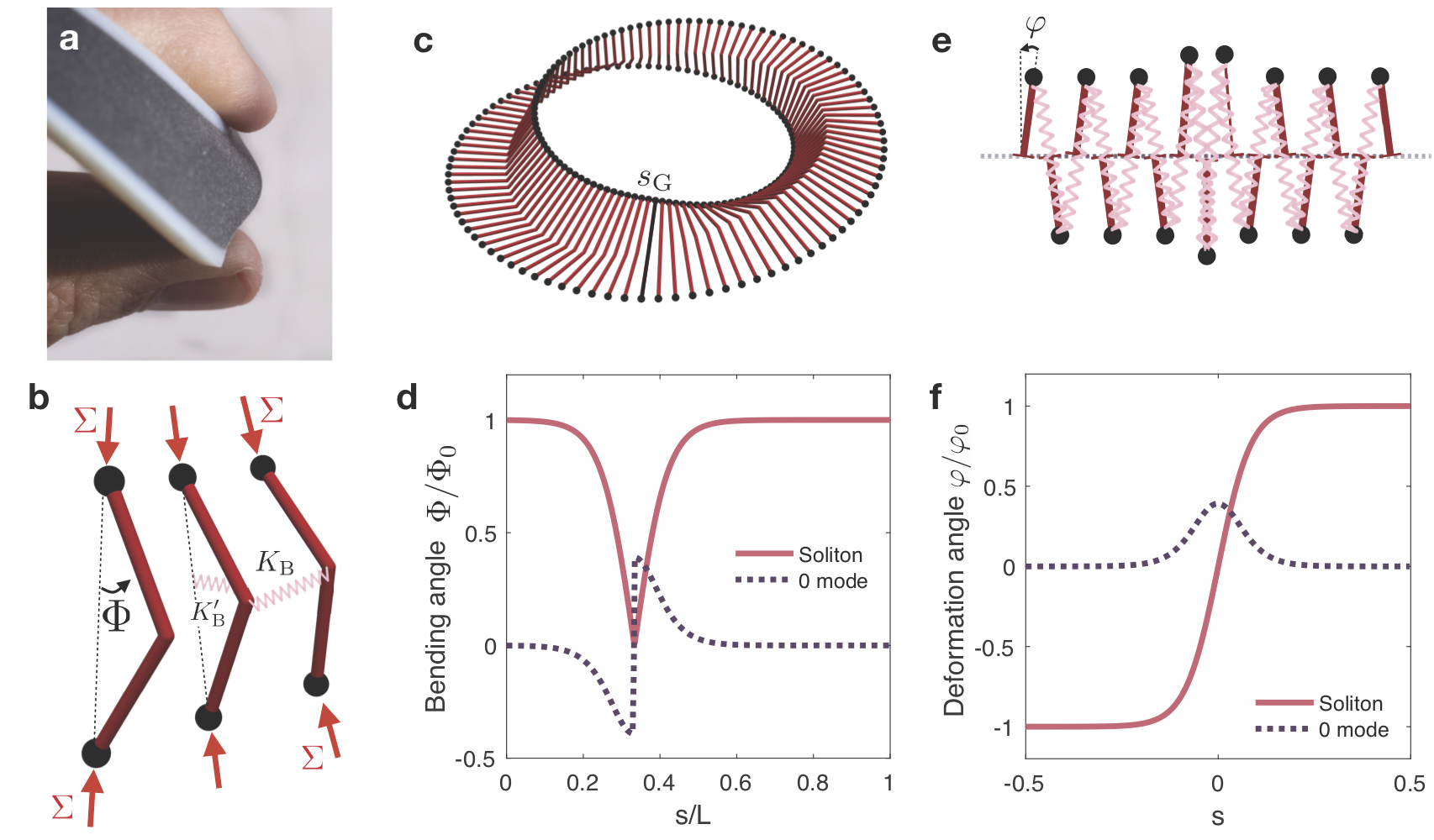
Figure 6: From buckled a Möbius strip to topological interface states. a. A 3D printed Möbius strip buckles upon application of a local compressive stress. b. Sketch of the simplified buckling-elasticity model. A Möbius ladder is composed of rigid bars of length $\ell$ connected by soft hinge of stiffness $K^{\prime}_{\rm B}$. The hinges are themselves coupled by harmonic springs of stiffness $K_{\rm B}$. The deformation of the $i^{\rm th}$ hinge is parametrized by the angle $\Phi_{i}$. $\Sigma$ indicates the strength of the applied compressive stress. c. Heterogeneous buckling pattern of a Möbius ladder. The location of the undeformed bar at $s=s_{\rm G}$ is indicated with a dark color. $\Phi_{0}=\pi/6$, $\xi=L/5$. d. Solid line: Shape of the soliton, i.e. variations of the bending angle $\Phi_{\rm B}(s)$. $s_{\rm G}$ topologically protect the strip from homogeneous bending. Dashed line: Shape of the floppy mode bound to the solitonic excitation. $\Phi_{0}=1$, $\xi=0.12L$. e. Sketch of the mechanical SSH model introduced in Kane and Lubensky (2014). This simple mechanicla metamaterial is composed of canted rigid bar free to rotate around a single axis are connected by harmonic springs, see Chen et al. (2014) for an experimental realization. f Solid line, the interface between two topologically distinct mechanical metamaterials is a $\phi^{4}$ kink. Dashed line: topological interface mode of the SSH model. $\varphi_{0}=1$, $\xi=0.12$.

III Buckling a Möbius strip

III.1 Solitary buckling waves

We now show how heterogeneous deformations emerge from homogeneous stresses. To do so, we address the consequences of non-orientability on the bending deformations of Möbius strips, see Fig. 6a. We consider a simplified description where the strip is modelled by a ladder made of flexible hinges of length $\ell$ as sketched in Fig. 6b. For sake of simplicity, we restrain ourselves to bending deformations along the normal vector which naturally couple to the ribbon orientation. The total elastic energy ${\mathcal{E}}_{\rm B}$ is composed of three terms: (i) the conformation the $i^{\rm th}$ hinge is defined by the angle $\Phi_{i}$ and is associated with a harmonic bending energy $\sim\frac{1}{2a}K_{\rm B}^{\prime}\Phi_{i}^{2}$, (ii) a harmonic coupling between the hinges adds a contribution $\sim\frac{1}{2a}K_{\rm B}(\Phi_{i+1}-\eta_{i,i+1}\Phi_{i})^{2}$, and (iii) applying an external compression load $\Sigma_{i}$ contributes to a mechanical work defined as the scalar product between the applied force and the resulting displacement: $(\Sigma_{i}a\ell)(\cos\Phi_{i}-1)$. We are now equipped to tackle the classical Euler buckling problem: the bending instability of a Möbius strip in response to a homogeneous compression. We first construct a continuum description of ${\mathcal{E}}_{\rm B}$ following the same procedure as in Section II.2, gauging away the $\eta_{i,i+1}$ variables, taking the continuum limit and restraining ourselves to deformations close to the onset of buckling. ${\mathcal{E}}_{\rm B}(\{\Phi\})$ then takes the compact form:

$${\mathcal{E}}_{\rm B}=\int\!\frac{K_{\rm B}}{2}\left(\partial_{s}\Phi\right)^{2}+U^{2}(\Phi)\,{\rm d}s\\ +(1-\mathcal{O})\lim_{a\to 0}\frac{K_{\rm B}}{a}\left(\Phi+a\Phi\partial_{s}\Phi\right)^{2}_{s=s_{\rm G}},$$ (5)

where the quartic potential

$$U(\Phi)=\frac{\sqrt{K_{\rm B}}}{\xi}(\Phi^{2}-\Phi_{0}^{2})$$ (6)

is classically parametrized by the scale $\xi^{2}=24a^{2}(K_{\rm B}/K^{\prime}_{\rm B})(\Sigma_{0}/\Sigma)$ over which bending deformations occur, and the distance to the critical buckling load of an isolated hinge: $\Phi_{0}^{2}=6(1-\Sigma_{\rm 0}/\Sigma)$, with $\Sigma_{\rm 0}a^{2}\equiv K^{\prime}_{\rm B}/\ell$. The last term of Eq. (5) is the gauge fixing term which constrains $\Phi(s)$ to vanish at a point $s_{\rm G}$, thereby protecting Möbius strips from homogeneous buckling. However, unlike shear stresses, the compression $\Sigma$ can be applied uniformly along the ribbon, and does not break translational invariance. $s_{\rm G}$ is then a free degree of freedom that parametrizes the broken-symmetry deformations.

The buckling patterns minimize ${\mathcal{E}}_{\rm B}$ with the constraint $\Phi(s_{\rm G})=0$. This minimization is performed using a dynamical-system analogy elaborated in Appendix B. In short, the strip remains flat until $\Sigma$ exceeds $\Sigma_{\rm c}=\Sigma_{0}\left[1+(K_{\rm B}/K^{\prime}_{\rm B})\pi^{2}(a/L)^{2}\right]$. Above $\Sigma_{\rm c}$ it undergoes a buckling transition and deforms into the inhomogeneous pattern illustrated in Fig. 6c. The bending angle $\Phi$ remains close to $\Phi_{0}$ everywhere except in a region of size $\xi/\Phi_{0}$ around $s_{\rm G}$ where it vanishes. The buckling pattern is the norm of a $\Phi^{4}$ kink centered on $s_{\rm G}$ Chaikin and C (1995). In the limit of long strips $\Phi_{\rm B}$ reduces to:

$$\Phi_{\rm B}(s-s_{\rm G})=\pm\Phi_{0}\left|\tanh\left(\frac{\sqrt{2}\Phi_{0}}{\xi}(s-s_{\rm G})\right)\right|+{\mathcal{O}}\left(\frac{\xi}{L}\right).$$ (7)

where the sign of the solution reflects the arbitrary choice of orientation of the ribbon. The exact solution beyond the very long strip approximation does not bring more insight and is left to Appendix B.

Remarkably, both the $\mathbb{Z}_{2}$ gauge symmetry and translational invariance are spontaneously broken at the onset of buckling. The ground state of $\mathcal{E}_{\rm B}$ is continuously degenerate leaving the bending direction and the location of the flat section $s_{\rm G}$ undetermined. As a consequence the buckling patterns are free to translate around the strips. More quantitatively, having macroscopic systems in mind, we now consider the inertial dynamics of the buckled strip described by the continuum Hamiltonian:

$${\mathcal{H}}_{\rm B}=\int\!\frac{I}{2}\left[(\partial_{t}\Phi)^{2}+\frac{K_{\rm B}}{2}(\partial_{s}\Phi)^{2}+U^{2}(\Phi)\right]\,{\rm d}s,$$ (8)

where $I$ is the local moment of inertia. As in the static case, ${\mathcal{H}}_{\rm B}$ is complemented by the constraint $\Phi(s_{\rm G}(t),t)$=0. The existence of solitary waves readily follows from the Lorentz invariance of ${\mathcal{H}}_{\rm B}$. The solitary waves are deduced from Eq.(7) by a Lorentz boost: $\Phi(s,t)=\Phi_{\rm B}(\gamma[s-vt])$, where $\gamma\equiv[1-(v/c)^{2}]^{-1/2}$ Chaikin and C (1995), and the propagation speed $v$ satisfies $v^{2}<c^{2}=K_{\rm B}/I$. The free propagation of these solitary bending waves restores translational and gauge invariance of Eq. (5): moving the topologically protected section $s_{\rm G}$ along the strip corresponds a mere gauge transformation which operates at zero energy cost. We note that travelling kinks of the very same nature were first found theoretically and illustrated experimentally in soap films forming non-orientable minimal surfaces  Machon et al. (2016). In the context of topological mechanics, spectacular zero-energy mechanisms having a similar solitonic structure were also found at the interface between open one-dimensional isostatic lattice having topologically distinct band spectra Chen et al. (2014); Vitelli et al. (2014). In the next section, we show that the latter resemblance is the first hint of a deeper connexion between the topological mechanics of non-orientable ribbons and that of one-dimensional isostatic metamaterials.

III.2 From buckled Möbius strips to SSH topological insulators

We characterized above the orientability of the ribbon by the invariant $\mathcal{O}$, and showed that $\mathcal{O}=-1$ implies the existence of solitary bending waves. Here, we show that these excitations are characterized by their own topological number $n$ which we relate to that of interface states between topological insulators. The standard topological characterization of both phononic and electronic excitation was established for lattice models and does not apply to continuous elasticity Mao and Lubensky (2018); Hasan and Kane (2010). We circumvent this technical obstacle following Ref. Vitelli et al., 2014. Resorting to an index theorem applied to the linearized elasticity of the strip, we establish that the soliton carries a topological charge $n=1$ that counts the zero energy translational modes.

In practice, we introduce the linear bending fluctuations of the ribbon around a static buckled state (7): $\Phi(s,t)=\Phi_{\rm B}(s-s_{\rm G})+\Psi(s,t)$, and deduce the dynamics of $\Psi$ by linearizing Eq. (8):

$$\partial^{2}_{t}\Psi(s,t)=-{\mathbb{D}}\Psi(s,t),$$ (9)

where ${\mathbb{D}}=\partial_{s}^{2}-2U^{\prime 2}(\Phi_{\rm B})-2U(\Phi_{B})U^{\prime\prime}(\Phi_{\rm B})$. The topological properties of mechanical vibrations are revealed by the ”square root” of the dynamical operator $\mathbb{D}$ Kane and Lubensky (2014). In the limit of very long yet finite ribbons, the dynamical operator can be recast into the factorized form (see Appendix C):

$$\mathbb{D}={\mathbb{Q}}^{\dagger}{\mathbb{Q}}+{\mathcal{O}}\left[(\xi/L)^{2}\right],$$ (10)

where ${\mathbb{Q}}^{\dagger}=\partial_{s}+\textrm{sign}(s-s_{\rm G})\sqrt{2}U^{\prime}(\Phi_{\rm B})$, and ${\mathbb{Q}}=-\partial_{s}+\textrm{sign}(s-s_{\rm G})\sqrt{2}U^{\prime}(\Phi_{\rm B})$. The soliton is then associated to the topological index $n$ that counts the zero modes of $\mathbb{D}$ making a distinction between floppy modes and self-stress states Kane and Lubensky (2014); Mao and Lubensky (2018); Vitelli et al. (2014):

$$n={\rm dim\,ker}\,{\mathbb{Q}}-{\rm dim\,ker}\,{\mathbb{Q}}^{\dagger}.$$ (11)

We compute $n$ by determining explicitly the kernel of the two linear operator ${\mathbb{Q}}$ and ${\mathbb{Q}}^{\dagger}$. In the limit $L/\xi\gg 1$ the corresponding eigenequations reduce to:

$$\partial_{s}\ln\Psi_{\pm}=\pm\partial_{s}\ln[\partial_{s}\Phi_{\rm B}(s)].$$ (12)

Solving Eq. (12) on the circle, we find that the kernel of ${\mathbb{Q}}^{\dagger}$ is trivial, while $\mathbb{Q}$ has a one-dimentional kernel: $\Psi_{+}=\delta s_{\rm G}\partial_{s}\Psi_{\rm G}$, where $\delta s_{\rm G}$ is a parametrization factor. This solution corresponds to an infinitesimal translation of the soliton: $\Psi_{+}(s;s_{\rm G})=\Phi_{\rm B}(s-s_{\rm G}-\delta s_{\rm G})-\Phi_{\rm B}(s-s_{\rm G})$ and is plotted in Fig. 6d. We stress that this translational mode is a floppy mode that operates, by definition, at zero energy cost. The topological index defined by Eq. (11) being non trivial ($n=1$), it ascertains the topological nature of the floppy modes and of the associated solitary wave.

This zero mode is reminiscent of the boundary states predicted by topological band theory at the interface between materials having topologically inequivalent eigenspaces Hasan and Kane (2010); Bernevig ; Kane and Lubensky (2014). These two types of zero modes are however essentially different. More precisely, Eqs. (9) and (10) are similar to the equations describing the vibrations of the interface between two SSH mechanical metamaterials illustrated in Fig. 6e, see Chen et al. (2014); Vitelli et al. (2014). In this different context, the existence of an interfacial zero mode is guaranteed by the imbalance between the number of self-stress and floppy modes given by the Kane-Lubensky generalization of the Maxwell-Caladine index Kane and Lubensky (2014). In the settings of Fig. 6e, the Kane-Lubensky count is equal to 1 thereby imposing the binding of a floppy mode to the interface. By contrast, the buckled Möbius ladder sketched in Fig. 6c is a closed isostatic system with a vanishing Maxwell-Caladine index. Therefore the existence of its zero mode is not captured by the Kane-Lubensky-Maxwell-Caladine index which disregards the gauge degrees of freedom associated to orientability. Beyond the specifics of mechancial systems, this counterintuitive observation prompts us to reconsider to very concept of the bulk-boundary correspondence of topological band theory when applied to non-orientable (meta)materials buckling solitons we identify are therefore intrinsically different from the edge state of a topological insulator embedded in the bulk of a lattice model defined on a Möbius strip as considered in: W. Beugeling et al. (20); Ryu ; Witten .

IV Conclusion and Perspectives

We have demonstrated how to surpass the native properties of materials without resorting to geometrical tuning. Constructing a minimal elastic theory for Möbius strips, we have established that non-orientability makes their local mechanics non-linear, non-reciprocal and capable of memorizing its stress history. Investigating their simplest bending instability, we have demonstrated how non-orientability guarantees the existence of a topological phase that supports zero-enery solitons. This mechanical phase, without known condensed-mater counterparts, begs for a generalization of the current bulk-boundary correspondance in topological materials Kitaev (2009); Ryu et al. (2010); Chiu et al. (2016); Zhang et al. (2019); Tang et al. (2019); Vergniory et al. (2019).

Our main predictions are elaborated building on prototypical models, we therefore expect their experimental implications to extend beyond the specifics of mechanical systems. In particular, the relation between nematic elasticity and ${\mathbb{Z}_{2}}$ gauge theories was realized in the early 90’s by Lammert et al. in the context of phase ordering, but to the best of our knowledge has remained virtually uncharted Lammert et al. (1995). We stress here that our central equation Eq. 3 also describes the Frank energy of non-orientable nematic films, and can be generalized to describe nematic elasticity around a disclination Alexander et al. (2012). A remarkable experimental realization of a non-orientable nematic liquid crystal was provided by self-assembled viral membranes where rod-like units self-organize into Möbius conformations at the membrane edge Gibaud et al. (2017). Beyond elasticity, we also envision our prediction to be relevant to Möbius configurations of light polarization Bauer et al. (2015); Bliokh et al. (2019), and to transport in twisted nano crystals Tanda et al. (2002).

acknowldegments

This work was supported by IdexLyon breakthrough program and ANR WTF grant. We thank Michel Fruchart and Krzysztof Gawedzki for stimulating discussions, William Irvine and Jeffrey Gustafson for help with the fabrications of Möbius strips, and Corentin Coulais for introducing us to nonreciprocal mechanics and for insightful suggestions. D.B. and D.C have equally contributed to all aspects of the research.

Appendix A Response to shear

A.1 No homogeneous shear stress

We showed in Section II.3 that a Möbius strip cannot support any homogeneous shear deformation. The situation is even more constrained as no uniform shear stress can be applied. The shear stress $\sigma^{\rm S}$ and $\theta^{\rm S}$ are conjugated variables, and the mechanical work associated to shear is given by ${\mathcal{W}}=-\int\sigma^{\rm S}(s)\theta^{\rm S}(s)\,\rm ds$. As $\mathcal{W}$ must be independent on the arbitrary definition of the ribbon orientation, $\sigma^{\rm S}$ and $\theta^{\rm S}$ must obey the same transformation rules upon any change in the ribbon orientation: $\sigma(s)$ is also topologically constrained to vanish at $s_{\rm G}$.

A.2 Response to a point-wise shear stress

We consider the response to the shear-stress distribution given by: $\sigma^{\rm S}=\sigma_{1}\delta(s-s_{1})$. For sake of clarity, units are here chosen so that $L=1$. The equilibrium configuration is obtained minimizing the total energy $\mathcal{E}+\mathcal{W}$ defined in Section II.3 with respect to both $\theta^{\rm S}$ and the gauge degree of freedom $s_{\rm G}$:

$$\mathcal{F}=\mathcal{E}+\mathcal{W}=\frac{K}{2}\int_{0}^{1}\left(\partial_{s}\theta^{\rm S}\right)^{2}-\int_{0}^{1}\sigma^{\rm S}(s)\theta^{\rm S}(s)\,\rm ds.$$ (13)

We recall that $s_{\rm G}$ is the location of the strip section where $\theta^{\rm S}(s)$ is topologically constrained to vanish. Within this framework, the two mechanical equilibrium conditions are:

$$\frac{\delta\mathcal{F}}{\delta\theta^{\rm S}} =-K\partial_{s}^{2}\theta^{\rm S}-\sigma^{\rm S}(s)=0,$$ (14)

$$\frac{\partial\mathcal{F}}{\partial s_{\rm G}} =0.$$ (15)

These equations are supplemented by the boundary conditions:

$$\theta^{\rm S}(s,s_{1};s_{\rm G})=\theta^{\rm S}(s+1,s_{1};s_{\rm G}),$$ (16)

and the topological constraint

$$\theta^{\rm S}(s=s_{\rm G},s_{1};s_{\rm G})=0.$$ (17)

The algebra is simplified by redefining the origin of the curvilinear coordinate ($s\to\tilde{s}$) such that $\tilde{s}_{\rm G}=0$. The conditions (16,17) then reduce to

$$\theta^{\rm S}(\tilde{s}=0,\tilde{s}_{1})=\theta^{\rm S}(\tilde{s}=1,\tilde{s}_{1}).$$ (18)

In this frame, the gauge degree of freedom then becomes the position of the applied stress $\tilde{s}_{1}=s_{1}-s_{\rm G}$ (mod $1$). Solving Eqs. 14 and 18, we readily find that the shear deformations are given by $\theta_{1}^{\rm S}(\tilde{s};\tilde{s}_{1})=\sigma_{1}G^{(1)}(\tilde{s};\tilde{s}_{1})$ with

$$G^{(1)}(\tilde{s};\tilde{s}_{1})=-\frac{1}{2K}\left(\left|\tilde{s}-\tilde{s}_{1}\right|+(\tilde{s}_{1}-1)\tilde{s}+(\tilde{s}-1)\tilde{s}_{1}\right).$$ (19)

The corresponding total energy

$$\mathcal{F}=-\frac{\sigma_{1}^{2}}{2K}\tilde{s}_{1}(1-\tilde{s}_{1})$$ (20)

is minimized for $\tilde{s}_{1}=\frac{1}{2}$, i.e. for $s_{\rm G}=s_{1}+\frac{1}{2}$ mod $1$. In other words, the point $s_{\rm G}$ where the shear deformation vanishes is maximally separated from the applied stress. Going back to the original frame, the static shear deformations at mechanical equilibrium are easily recast into:

$$\theta_{1}(s,s_{1})=\frac{\sigma_{1}}{2K}\left|s-s_{1}-\frac{1}{2}\operatorname{sgn}(s-s_{1})\right|,$$ (21)

which corresponds to Eq. 4 in the main text.

A.3 Response to $N$ localized shear sources

We now consider the superposition of $N$ fixed point-wise sources : $\sigma^{\rm S}(s)=\sum_{i=1}^{N}\sigma_{i}\delta(s-s_{i})$. The equilibrium conformation $\theta^{\rm S}_{N}(s,\{s_{i}\};s_{\rm G})$ of the Möbius strip satisfies the condition (14,15) with the boundary conditions (16,17). Working in the frame where $s_{\rm G}=0$, the solution of this equation is

$$\theta_{N}^{\rm S}(\tilde{s};\{\tilde{s}_{i}\})=\sum_{i=1}^{N}\sigma_{i}~{}G^{(1)}(\tilde{s};\tilde{s}_{i}),$$ (22)

where $\tilde{s}_{i}=s_{i}-s_{\rm G}$ mod $(1)$, i.e. $\tilde{s}_{i}=s_{i}-s_{\rm G}+\Theta(s_{\rm G}-s_{i})$ where $\Theta(s)$ is the Heaviside step function. At first sight Eq. 22 resembles the mere superposition of independent Green functions and suggests a typical linear response behavior. However we have to keep in mind that the position $s_{\rm G}$ is yet to be determined to prescribe the equilibrium deformations. As a shift in the position $s_{\rm G}$ corresponds to a uniform translation of all the stress sources. we need to compute the equilibrium value of $\tilde{s}_{1}$, keeping all distances $\tilde{s}_{i}-\tilde{s}_{1}$ fixed. Inspired by the classical calculation of the elastic interactions between inclusions in soft membranes and liquid interfaces (see e.g. Bartolo and Fournier (2003)), we integrate over the shear degrees of freedom and derive the effective potential $U_{N}(s_{\rm G})$ that controls the position of $s_{\rm G}$ along the strip. To compute $U_{N}$, it is convenient to solve a seemingly more complex problem where the strip undergoes thermal fluctuations. The thermal statistics is then defined by the partition function

$$\mathcal{Z}[\{\sigma_{i}\}]=\int_{0}^{1}{\rm d}s_{\rm G}\int\!{\mathcal{D}}\theta^{\rm S}\\ e^{-\beta\left[\int\!{\rm d}\tilde{s}\,\frac{1}{2}(\partial_{\tilde{s}}\theta^{\rm S})^{2}-\sum_{i}\sigma_{i}\theta^{\rm S}(\tilde{s}_{i})\right]},$$ (23)

where $\beta^{-1}\equiv K_{\rm B}T$ and the field $\theta^{\rm S}(\tilde{s})$ satisfies the condition (18). Integrating out the $\theta^{\rm s}$ degrees of freedom defines the effective potential $U_{N}(s_{\rm G})$:

$$\mathcal{Z} =\int_{0}^{1}\!{\rm d}s_{\rm G}\,e^{-\beta U_{N}(s_{\rm G})},$$ (24)

$$\mathrm{with}\ \ U_{N}(s_{\rm G}) =-\frac{1}{2}\sum_{i,j}\sigma_{i}\sigma_{j}~{}G^{(1)}(\tilde{s}_{i},\tilde{s}_{j}).$$ (25)

Going back to the original mechanics problem, i.e. taking the zero temperature limit in Eq. 25, we find the equilibrium position of $s_{\rm G}=0$ by minimizing $U_{N}(s_{\rm G})$. The non-linearity of the shear response of the Möbius strip originates from this last minimization procedure, which translates the topological constraint.

Figure 7: Equilibrium positions of $s_{\rm G}$. Effective potential $U_{2}(s_{\rm G})$ trapping the position of $s_{\rm G}$ along the strip when two identical shear stresses are applied at positions $s_{1},s_{2}$. The blue circles indicate the two locally stable positions of $s_{\rm G}$. $U_{2}$ is minimized when $s_{\rm G}$ is maximally distant from the appleid stresses. Illustration with $s_{1}=1/10$ and $s_{2}=1/2$ and $\sigma_{1}=\sigma_{2}=K$.

We illustrate this method for two identical stress sources located at $s_{1}$ and $s_{2}$ separated by a constant distance $\Delta$: $\sigma^{\rm s}(s)=\sigma\left[\delta(s-s_{1})+\delta(s-s_{2})\right]$, with $s_{2}=(s_{1}+\Delta)\,{\rm mod}(1)$ and find

$$U_{2}(s_{\rm G})=\\ \frac{\sigma^{2}}{2K}\left(|\tilde{s}_{2}-\tilde{s}_{1}|+(\tilde{s}_{1}+\tilde{s}_{2})(\tilde{s}_{1}+\tilde{s}_{2}-2)\right)$$ (26)

Minimizing $U_{2}(s_{\rm G})$, we find two local minima satisfying $\partial_{s_{\rm G}}U_{2}=0$ at $s_{\rm G}=(s_{1}+s_{2})/2$ mod $(1)$ and $s_{\rm G}=(s_{1}+s_{2})/2+\frac{1}{2}$ mod $(1)$. They are sketched in Fig. 7 and reflect the mirror symmetry of the problem. The lowest energy conformation always corresponds to the value of $s_{\rm G}$ the further away from the stress sources. In the symmetric case, where $\Delta=\frac{1}{2}$, the shear response possesses two degenerate equilibrium positions. With the knowledge of the position $s_{\rm G}$ the shear-deformation profile is fully determined. It is given by Eq. (22), and illustrated in Fig. 3 for various positions of $s_{1},s_{2}$.

Appendix B Buckling patterns and solitary waves, a dynamical-system insight.

We compute the shape of buckled Möbius strips making use of a dynamical system analogy. The expression of the elastic energy given by Eq. (5) is indeed analogous to the Lagrangian of a classical particle of unit mass, and moving in a potential $V(\Phi)=-\xi^{-2}(\Phi^{2}-\Phi_{0}^{2})^{2}$, where $\Phi$ indicates the particle position, $s$ the time, and $\partial_{s}\Phi$ the particle velocity, see Fig. 8. Both the non-orientability constraint, and the finite size of the strip complexifies the dynamics of this seemingly simple dynamical system. We show below that the trajectories are not periodic and singular at $s_{\rm G}$.

Without loss of generality we chose $s_{\rm G}=0$. Non-orientability therefore implies that $\Phi(0)=\Phi(L)=0$ regardless of the value of the particle speed $\partial_{s}\Phi(s_{\rm G})$. The trajectory $\Phi(s)$ is found noting that the mechanical energy $E_{\rm m}=\frac{1}{2}[\partial_{s}\Phi(s)]^{2}+V[\Phi(s)]$ is a constant of motion. Noting $\Phi_{\rm m}=\max[\Phi(s)]$, the periodicity of the trajectory (reflecting the periodicity of the strip shape) imposes $|\Phi_{\rm m}|<\Phi_{0}$. Otherwise, one would simultaneously have $\partial_{s}\Phi=0$ and $\Phi>\Phi_{0}$, thereby leading to runaway solutions. Invariance upon time reversal of the particle Lagragian also imposes $\Phi_{\rm m}=\Phi(L/2)$. Therefore, the conservation of mechanical energy implies:

$$\partial_{s}\Phi(s)=\pm{\sqrt{2[V(\Phi_{\rm m})-V(\Phi(s))]}}.$$ (27)

Let us consider solutions where $\Phi_{\rm m}>0$. The sign of $\partial_{s}\Phi(s)$ in Eq. (27) is then positive when $0<s<L/2$ and negative when $L/2<s<L$, and the inverse function $s=\Phi^{-1}[\Phi(s)]$ is readily found integrating Eq. (27) on the two separate intervals:

$$s =\pm\xi\int_{0}^{\Phi}\frac{{\rm d}x}{\sqrt{2(x^{2}-\Phi_{\rm m}^{2})(x^{2}+\Phi_{\rm m}^{2}-2\Phi_{0}^{2})}},$$

$$=\xi\frac{1}{\sqrt{4\Phi_{0}^{2}-2\Phi_{\rm m}^{2}}}F[\arcsin(\Phi/\Phi_{\rm m},k)],$$ (28)

where $k\equiv\Phi_{\rm m}^{2}/(2\Phi_{0}^{2}-\Phi_{\rm m}^{2})$ and $F(x,k)$ is the incomplete elliptic integral of the first kind. The final form of the trajectory follows from the definition $\Phi_{\rm m}\equiv\Phi(1/2)$ which imposes $\Phi_{\rm m}^{2}=2\Phi_{0}^{2}-2(\xi L^{-1})F(\pi/2,k)$. We stress that our gauge choice constraints $\phi(s)$ to vanish at $s_{\rm G}=0$ thereby imposing the derivative of $\Phi$ to be discontinuous at $s_{\rm G}$. The solution corresponds to two symmetric half $\Phi^{4}$ kinks defined on a compact interval is plotted in Fig. 6d in the main text. One last comments is in order. In the limit of large ribbons assembled from very stiff hinges, $\xi/L\ll 1$, $\Phi_{\rm m}=\Phi_{0}$, and the integration of Eq. (27) results in the usual $\tanh$ profiles given by Eq. (7). The buckling pattern corresponds to the symetrization of the usual $\Phi^{4}$ soliton.

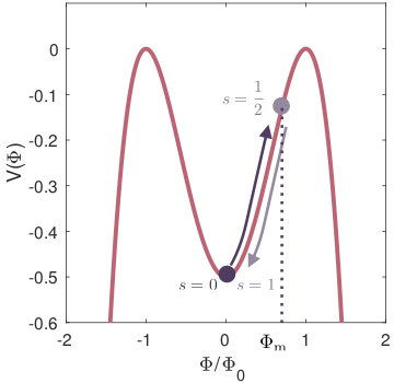
Figure 8: Soliton shape: kicked particle in a potential. The potential $V(\Phi)$ is plotted versus $\Phi$. At time $s=0$ the particle is located in the potential well (dark circle). It is however not at rest as its velocity is non zero; it is kicked uphill and reaches its maximal position at $s=\frac{1}{2}$ (light circle). It then falls back to its initial position at $t=1$. The particle speed at $s=0$ and $s=1$ are opposite. $\Phi_{0}=1/2$, $\xi=1$. This feature translates into a slope discontinuity of the soliton shape at $s_{\rm G}$.

Appendix C Factorization of the dynamical operator.

We show how to factorize the dynamical operator ${\mathbb{D}}=\partial_{s}^{2}-2U^{\prime 2}(\Phi_{\rm 0})-2U(\Phi_{\rm 0})U^{\prime\prime}(\Phi_{\rm 0})$ defined in Eq. (9). As discussed above in Appendix B, in the limit of infinitely long ribbons, $\Phi^{\infty}_{\rm m}=\Phi_{0}$ and $V(\Phi_{\rm m}^{\infty})=E_{\rm m}=0$. The latter relation simplifies Eq. (27):

$$\partial_{s}\Phi^{\infty}(s)=\textrm{sgn}(s-s_{\rm G})\sqrt{2}U[\Phi^{\infty}(s)].$$ (29)

Together with the definition of $\mathbb{D}$, this relation implies the factorization $\mathbb{D}={\mathbb{Q}}^{\dagger}{\mathbb{Q}}$, with

$${\mathbb{Q}}^{\dagger} =\partial_{s}+\textrm{sgn}(s-s_{\rm G})\sqrt{2}U^{\prime}(\Phi^{\infty}_{\rm 0}),$$ (30)

$${\mathbb{Q}} =-\partial_{s}+\textrm{sgn}(s-s_{\rm G})\sqrt{2}U^{\prime}(\Phi^{\infty}_{\rm 0}),$$ (31)

where $\Phi^{\infty}_{0}$ is the shape of the unperturbed buckled ribbon. A $\xi/L$ expansion shows that this form is preserved for very long but finite ribbons. This result is obtained expressing the ribbon shape as a linear perturbation of $\Phi^{\infty}$: $\Phi_{0}=\Phi_{\rm 0}^{\infty}+(\xi/L)\tilde{\Phi}$. Evaluating $E_{\rm m}$, and keeping in mind that $U(\Phi_{0})=0$, we find: $E_{\rm m}=U^{2}(\Phi_{0}+\tilde{\Phi}_{\rm m})=U^{2}(\Phi_{0})+2U(\Phi_{0})U^{\prime}(\Phi_{0})\tilde{\Phi}_{\rm m}+{\mathcal{O}}[(\xi/L)^{2}]={\mathcal{O}}[(\xi/L)^{2}]$. The relations $E_{\rm m}=0$ and Eq. (29) are hence preserved at first order in $\xi/L$. Therefore, even though the Hamiltonian $\mathcal{H}_{\rm B}$ defined in Eq.(8) does not enjoy the BPS symmetry of the continuum description of the isostatic chain of linkages introduced in Vitelli et al. (2014), the corresponding dynamical matrix can still be factorized as $\mathbb{D}={\mathbb{Q}}^{\dagger}{\mathbb{Q}}$, substituting $\Phi^{\infty}$ by $\Phi$ in Eqs. (30) and Eqs. (31).

References

- Kvavadze et al. (2009) Eliso Kvavadze, Ofer Bar-Yosef, Anna Belfer-Cohen, Elisabetta Boaretto, Nino Jakeli, Zinovi Matskevich, and Tengiz Meshveliani, “30,000-year-old wild flax fibers,” Science 325, 1359–1359 (2009).
- Bertoldi et al. (2017) Katia Bertoldi, Vincenzo Vitelli, Johan Christensen, and Martin van Hecke, “Flexible mechanical metamaterials,” Nature Reviews Materials 2, 17066 (2017).
- Kane and Lubensky (2014) C. L. Kane and T. C. Lubensky, “Topological boundary modes in isostatic lattices,” Nature Physics 10, 39 (2014).
- Prodan and Prodan (2009) Emil Prodan and Camelia Prodan, “Topological phonon modes and their role in dynamic instability of microtubules,” Physical review letters 103, 248101 (2009).
- Süsstrunk and Huber (2015) Roman Süsstrunk and Sebastian D Huber, “Observation of phononic helical edge states in a mechanical topological insulator,” Science 349, 47–50 (2015).
- Nash et al. (2015) Lisa M Nash, Dustin Kleckner, Alismari Read, Vincenzo Vitelli, Ari M Turner, and William TM Irvine, “Topological mechanics of gyroscopic metamaterials,” Proceedings of the National Academy of Sciences 112, 14495–14500 (2015).
- Huber (2016) Sebastian D Huber, “Topological mechanics,” Nature Physics 12, 621 (2016).
- Mao and Lubensky (2018) Xiaoming Mao and Tom C Lubensky, “Maxwell lattices and topological mechanics,” Annual Review of Condensed Matter Physics 9, 413–433 (2018).
- Chen et al. (2014) Bryan Gin-ge Chen, Nitin Upadhyaya, and Vincenzo Vitelli, “Nonlinear conduction via solitons in a topological mechanical insulator,” Proceedings of the National Academy of Sciences 111, 13004–13009 (2014).
- Barlas and Prodan (2018) Yafis Barlas and Emil Prodan, “Topological meta-materials: An algorithmic design,” arXiv preprint arXiv:1805.05828 (2018).
- Süsstrunk and Huber (2016) Roman Süsstrunk and Sebastian D Huber, “Classification of topological phonons in linear mechanical metamaterials,” Proceedings of the National Academy of Sciences 113, E4767–E4775 (2016).
- Mitchell et al. (2018) Noah P. Mitchell, Lisa M. Nash, Daniel Hexner, Ari M. Turner, and William T. M. Irvine, “Amorphous topological insulators constructed from random point sets,” Nature Physics , 1 (2018).
- Hasan and Kane (2010) M. Zahid Hasan and Charles L. Kane, “Colloquium: topological insulators,” Reviews of Modern Physics 82, 3045 (2010).
- (14) Andrei B. Bernevig and Taylor L. Hughes, Topological insulators and topological superconductors, Princeton university press, (2013).
- (15) For a recent generalization see Kai Sun and Xiaoming Mao, arXiv preprint arXiv:1907.13163, 2019.
- Audoly and Pomeau (2010) Basile Audoly and Yves Pomeau, Elasticity and geometry: from hair curls to the non-linear response of shells (Oxford University Press, 2010).
- Kamien (2002) Randall D. Kamien, “The geometry of soft materials: a primer,” Rev. Mod. Phys. 74, 953–971 (2002).
- Note (1) Note that an alternative description consists in allowing to be discontinuous. The topological term would then imposes : shear deformations would be antiperiodic functions of .
- Maxwell (1864) J. Clerk Maxwell, “On the calculation of the equilibrium and stiffness of frames,” The London, Edinburgh, and Dublin Philosophical Magazine and Journal of Science 27, 294–299 (1864).
- Betti (1872) Enrico Betti, “Teoria della elasticita,” Il Nuovo Cimento (1869-1876) 7, 158–180 (1872).
- Coulais et al. (2017) Corentin Coulais, Dimitrios Sounas, and Andrea Alù, “Static non-reciprocity in mechanical metamaterials,” Nature 542, 461 (2017).
- Chaikin and C (1995) Paul M Chaikin and Lubensky Tom C, Principles of condensed matter physics, Vol. 1 (Cambridge university press Cambridge, 1995).
- Machon et al. (2016) Thomas Machon, Gareth P. Alexander, Raymond E. Goldstein, and Adriana I. Pesci, “Instabilities and solitons in minimal strips,” Phys. Rev. Lett. 117, 017801 (2016).
- Vitelli et al. (2014) Vincenzo Vitelli, Nitin Upadhyaya, and Bryan Gin-ge Chen, “Topological mechanisms as classical spinor fields,” arXiv preprint arXiv:1407.2890 (2014).
- buckling solitons we identify are therefore intrinsically different from the edge state of a topological insulator embedded in the bulk of a lattice model defined on a Möbius strip as considered in: W. Beugeling et al. (20) The buckling solitons we identify are therefore intrinsically different from the edge state of a topological insulator embedded in the bulk of a lattice model defined on a Möbius strip as considered in: W. Beugeling, A. Quelle, and C. Morais Smith, “Nontrivial topological states on a möbius band,” Phys. Rev. B 89, 235112 (2014).
- (26) AtMa P.O. Chan, Jeffrey C. Y. Teo, and Shinsei Ryu, ”Topological phases on non-orientable surfaces: twisting by parity symmetry.” New Journal of Physics 18.3, 035005 (2016) .
- (27) Witten, Edward Witten, ”Fermion path integrals and topological phases”, Reviews of Modern Physics 88, 035001 (2016).
- Kitaev (2009) Alexei Kitaev, “Periodic table for topological insulators and superconductors,” in AIP Conference Proceedings, Vol. 1134 (AIP, 2009) pp. 22–30.
- Ryu et al. (2010) Shinsei Ryu, Andreas P Schnyder, Akira Furusaki, and Andreas W. W. Ludwig, “Topological insulators and superconductors: tenfold way and dimensional hierarchy,” New Journal of Physics 12, 065010 (2010).
- Chiu et al. (2016) Ching-Kai Chiu, Jeffrey C. Y. Teo, Andreas P. Schnyder, and Shinsei Ryu, “Classification of topological quantum matter with symmetries,” Rev. Mod. Phys. 88, 035005 (2016).
- Zhang et al. (2019) Tiantian Zhang, Yi Jiang, Zhida Song, He Huang, Yuqing He, Zhong Fang, Hongming Weng, and Chen Fang, “Catalogue of topological electronic materials,” Nature 566, 475 (2019).
- Tang et al. (2019) Feng Tang, Hoi Chun Po, Ashvin Vishwanath, and Xiangang Wan, “Comprehensive search for topological materials using symmetry indicators,” Nature 566, 486–489 (2019).
- Vergniory et al. (2019) MG Vergniory, L Elcoro, Claudia Felser, Nicolas Regnault, B Andrei Bernevig, and Zhijun Wang, “A complete catalogue of high-quality topological materials,” Nature 566, 480 (2019).
- Lammert et al. (1995) Paul E Lammert, Daniel S Rokhsar, and John Toner, “Topology and nematic ordering. i. a gauge theory,” Physical Review E 52, 1778 (1995).
- Alexander et al. (2012) Gareth P. Alexander, Bryan Gin-ge Chen, Elisabetta A. Matsumoto, and Randall D. Kamien, “Colloquium: Disclination loops, point defects, and all that in nematic liquid crystals,” Rev. Mod. Phys. 84, 497–514 (2012).
- Gibaud et al. (2017) Thomas Gibaud, C Nadir Kaplan, Prerna Sharma, Mark J Zakhary, Andrew Ward, Rudolf Oldenbourg, Robert B Meyer, Randall D Kamien, Thomas R Powers, and Zvonimir Dogic, “Achiral symmetry breaking and positive gaussian modulus lead to scalloped colloidal membranes,” Proceedings of the National Academy of Sciences 114, E3376–E3384 (2017).
- Bauer et al. (2015) Thomas Bauer, Peter Banzer, Ebrahim Karimi, Sergej Orlov, Andrea Rubano, Lorenzo Marrucci, Enrico Santamato, Robert W Boyd, and Gerd Leuchs, “Observation of optical polarization möbius strips,” Science 347, 964–966 (2015).
- Bliokh et al. (2019) Konstantin Y Bliokh, Miguel A Alonso, and Mark R Dennis, “Geometric phases in 2d and 3d polarized fields: geometrical, dynamical, and topological aspects,” arXiv preprint arXiv:1903.01304 (2019).
- Tanda et al. (2002) Satoshi Tanda, Taku Tsuneta, Yoshitoshi Okajima, Katsuhiko Inagaki, Kazuhiko Yamaya, and Noriyuki Hatakenaka, “Crystal topology: A möbius strip of single crystals,” Nature 417, 397 (2002).
- Bartolo and Fournier (2003) Denis Bartolo and J-B Fournier, “Elastic interaction between” hard” or” soft” pointwise inclusions on biological membranes,” The European Physical Journal E 11, 141–146 (2003).