The evolution of carbon-polluted white dwarfs at low effective temperatures

Abstract

Taking advantage of the Gaia Data Release 2, recent studies have revisited the evolution of carbon-polluted white dwarfs (DQs) across a large range of effective temperatures. These analyses have clearly confirmed the existence of two distinct DQ evolutionary sequences: one with normal-mass white dwarfs and one with heavily polluted and generally more massive objects. The first sequence is thought to result from the dredge-up of carbon from the core, while the second could at least partially be made of descendants of Hot DQs. However, the evolution of carbon-polluted white dwarfs below 6500 K remains unexplored, mainly due to the theoretical difficulties associated with modelling their dense atmospheres. In this work, we present a detailed star-by-star analysis of cool carbon-polluted white dwarfs. Our recently improved atmosphere models allow us to obtain good fits to most objects, including very cool DQpec white dwarfs with strongly shifted C₂ molecular bands. We show that cool carbon-polluted white dwarfs keep following the two distinct evolutionary tracks previously identified at higher temperatures. We also find that most DQ white dwarfs transform into DQpec when their photospheric densities exceed $\approx 0.15\,{\textrm{g\,cm}}^{-3}$. However, we identify stars for which the DQ$\rightarrow$DQpec transition occurs at lower photospheric densities, possibly due to the presence of a strong magnetic field.

1 Introduction

A DQ star is a white dwarf whose spectrum is dominated by carbon features. Depending on the effective temperature of a DQ white dwarf, the spectroscopic signature of carbon can take different forms. For warm DQ white dwarfs ($T_{\rm eff}\approx 10{,}000-16{,}000\,{\rm K}$), carbon is detected as C i atomic lines. At lower temperatures ($T_{\rm eff}<10{,}000\,{\rm K}$), the formation of the C₂ molecule leads to the appearance of strong molecular bands, the most prominent being the Swan bands ($4500-6000\,{\AA}$). Spectroscopic analyses of cool DQ white dwarfs using atmosphere models have shown that the atmosphere of those objects is dominated by helium and polluted by small quantities of carbon ($-7<\log\,{\rm C/He}<-2$, e.g., Koester et al., 1982; Weidemann & Koester, 1995; Dufour et al., 2005; Koester & Knist, 2006). The presence of carbon in the atmosphere of DQ stars implies the existence of a mechanism that thwarts the efficient gravitational settling at play in white dwarfs. For most DQs, this mechanism is the transport of carbon from the deep interior by the helium convection zone (Pelletier et al., 1986; Fontaine & Brassard, 2005). In fact, for the bulk of objects, the observed monotonic decrease of $\log\,{\textrm{C/He}}$ with decreasing $T_{\rm{eff}}$ (Dufour et al., 2005; Koester & Knist, 2006; Kepler et al., 2016) is well accounted for by this model (e.g., Coutu et al., 2019, Figure 12).

However, the dredge-up model fails to explain the observed composition of a second sequence of DQ white dwarfs that, for a given $T_{\rm eff}$, have carbon abundances about one order of magnitude higher than the main DQ sequence (e.g., Coutu et al., 2019, Figure 12). As clearly revealed by the Gaia DR2 parallaxes, above $T_{\rm eff}\approx 10{,}000\,{\rm K}$, this second sequence is made of more massive objects ($\langle M\rangle\approx 1\,M_{\odot}$, Coutu et al., 2019; Koester & Kepler, 2019). The problem is that high-mass evolutionary sequences simply cannot match the slope of the observed decrease of $\log\,{\textrm{C/He}}$ with decreasing $T_{\rm{eff}}$ (Brassard et al., 2007, Figure 1). The fact that evolutionary models fail to account for the atmospheric composition of those objects—while successfully accounting for the composition of DQs on the first sequence—clearly suggests that another scenario than the dredge-up model must be invoked to explain carbon pollution in the second sequence. The preferred scenario is that they are the product of the evolution of another white dwarf spectral type, Hot DQs (Coutu et al., 2019). The spectra of Hot DQ white dwarfs are characterized by C i and C ii atomic lines (Liebert et al., 2003). Model atmosphere analyses have shown that those stars have carbon-dominated atmospheres and effective temperatures ranging from $18{,}000$ to $24{,}000\,{\rm K}$ (Dufour et al., 2007, 2008). Hot DQ white dwarfs are thought to originate from merged white dwarfs (Dunlap, 2015; Dunlap & Clemens, 2015). This hypothesis is supported by the high velocity dispersion of those objects, which suggests that they are much older than the age inferred from their atmospheric parameters. As a merger event would lead to a significant reheating, the cooling age derived from the temperature becomes meaningless, which naturally explains the mismatch with the kinematic age. Many pieces of evidence support the idea that, at least above $T_{\rm eff}\approx 10{,}000\,{\rm K}$, the second DQ sequence is made of the descendants of Hot DQs: (1) the second sequence connects nicely with the Hot DQs in a $T_{\rm eff}-\log\,{\rm C/He}$ diagram (Dufour et al., 2013; Coutu et al., 2019), thus suggesting a common evolutionary origin; (2) DQs from the second sequence have similar kinematic properties as Hot DQs (Dunlap & Clemens, 2015; Coutu et al., 2019); (3) both populations are characterized by high masses (Dunlap et al. submitted, Coutu et al., 2019).

The very recent studies of Coutu et al. (2019) and Koester & Kepler (2019) represent an important step forward in our understanding of the evolution of carbon-polluted white dwarfs. However, their analyses stop short of investigating the evolution of DQ white dwarfs at very cool effective temperatures ($T_{\rm eff}<6500\,{\rm K}$). Cool, helium-rich white dwarf atmospheres are characterized by high photospheric densities (e.g., Blouin et al., 2017, Figure 13). Under such conditions, the radiative opacities, the equation of state and the chemical equilibrium can significantly differ from the ideal gas results (Kowalski & Saumon, 2006; Kowalski et al., 2007; Blouin et al., 2018a; Rohrmann, 2018). In particular, the C₂ Swan bands undergo a density-driven distortion that has been attributed to a shift of the electronic transition energy (Kowalski, 2010). White dwarfs with such distorted Swan bands are known as DQpec stars (Hall & Maxwell, 2008). For a lack of atmosphere models accounting for those high-density effects, Coutu et al. (2019) have ignored all DQpec white dwarfs from their analysis as well as all DQs with an effective temperature below 6000 K. Regarding the study of Koester & Kepler (2019), a crude analysis of DQpec white dwarfs was performed assuming a constant effective temperature and carbon abundance for all objects. Based on this analysis, they concluded that DQpec white dwarfs might be massive objects that are the descendants of the Hot DQs.

The aim of this work is to establish the evolution of DQ white dwarfs at very cool effective temperatures ($T_{\rm eff}<6500\,{\rm K}$). This is done using our recently improved atmosphere models and a sample of all known cool DQ white dwarfs. Our models and the selection of our sample are described in Section 2. We present our model atmosphere analysis in Section 3 and the implications of our results on the evolution of carbon-polluted white dwarfs in Section 4. Finally, our main conclusions are given in Section 5.

2 Methodology

2.1 Atmosphere models

The atmosphere code used in this work is identical to that described in Blouin et al. (2019). This code is uniquely suited for the study of cool helium-rich white dwarfs as it includes an accurate description of the effects of a high helium density on the chemical equilibrium and on the radiative opacities (Blouin et al., 2018a; Blouin et al., 2018b, and references therein). The opacity of the C₂ Swan bands is computed with a line-by-line approach that uses a linelist provided by J. O. Hornkohl (private communication), which was obtained following the methodology described in Parigger et al. (2015). Moreover, following the work of Kowalski (2010), we include a density-driven shift of the electronic transition energy of the Swan bands. This shift is computed as $\Delta T_{e}(\rm eV)=\alpha\rho(\textrm{g\,cm}^{-3})$, where $\alpha=0.2$ as empirically determined in Blouin et al. (2019, Section 3.3). We use a 3-dimensional grid of model atmospheres, with $T_{\rm{eff}}$ varying from 4000 K to 9000 K in steps of 500 K, $\log g$ from 7.0 to 9.0 in steps of 0.5 dex, and $\log\,{\textrm{C/He}}$ from $-9.0$ to $-4.0$ in steps of 0.5 dex. Note that our models do not include any hydrogen. This is justified by the finding that for $T_{\rm eff}<8000\,{\rm K}$ the CH $G$ band should be visible even for hydrogen abundances that lead to a negligible impact on the model and on the derived atmospheric parameters (Blouin et al., 2019; Coutu et al., 2019). Only one object in our sample, G99$-$37 (GJ 1086), displays a CH $G$ band. For this object, we rely on the solution already provided in Blouin et al. (2019).

One major caveat of our models is the current uncertainty surrounding ultraviolet opacities. The carbon atomic lines are included using the Vienna Atomic Line Database (VALD, Piskunov et al., 1995; Kupka et al., 1999; Ryabchikova et al., 2015). However, as discussed in Coutu et al. (2019) and Koester & Kepler (2019), many carbon lines in the ultraviolet are predicted to be much stronger and wider than they appear in observed spectra. This problem is probably at the origin of a $\approx 0.05\,M_{\odot}$ shift of the peak of the DQ mass distribution with respect to that of DA and DB white dwarfs (Coutu et al., 2019). This finding casts some doubts on the absolute values of the derived atmospheric parameters, but the effect on the relative values between objects is expected to be minimal.

Table 1: Observational data.

SDSS J	MWDD ID	SDSS					Pan–STARRS					$\pi$	$\sigma_{\pi}$	Spectrum	Magnetic?
		$u$	$g$	$r$	$i$	$z$	$g$	$r$	$i$	$z$	$y$	(mas)	(mas)	source
–	GJ 2012	–	–	–	–	–	14.76	14.29	14.11	14.06	14.03	109.88	0.03	(1)	No ($<3\,{\rm MG}$)a
–	LP 410$-$80	–	–	–	–	–	17.17	16.91	16.91	16.93	16.99	23.71	0.09	(2)
–	Wolf 219	–	–	–	–	–	15.28	15.08	15.06	15.15	15.14	53.00	0.05	(1)	Nob
–	LP 717$-$1	–	–	–	–	–	17.55	17.04	16.88	16.86	16.83	28.83	0.08	(2)
–	GJ 1086	–	–	–	–	–	14.77	14.40	14.35	14.39	14.44	89.17	0.03	(1)	$\approx 7.5\,{\rm MG}^{c}$
080455.42+171443.6	SDSS J080455.42+171443.6	19.92	19.05	18.46	18.26	18.23	18.99	18.44	18.29	18.25	18.22	14.95	0.33	SDSS
080558.84+072448.5	SDSS J080558.83+072447.8	20.45	19.55	18.89	18.69	18.66	19.48	18.89	18.72	18.66	18.72	12.80	0.35	SDSS
080843.15+464028.6	WD 0805+468	20.69	20.37	19.35	19.10	19.03	20.40	19.42	19.13	19.15	19.23	9.67	0.72	SDSS
082955.77+183532.6	[VV2010c] J082955.8+183532	22.74	21.82	20.45	20.17	20.18	21.68	20.46	20.20	20.03	20.02	5.74	1.75	SDSS
083618.13+243254.6	SDSS J083618.13+243254.6	20.30	19.51	18.90	18.74	18.70	19.48	18.94	18.73	18.75	18.65	10.23	0.93	SDSS
090208.40+201049.9	LP 426-49	18.95	18.87	17.79	17.25	17.29	18.90	17.75	17.26	17.30	17.36	25.92	0.17	SDSS
090632.17+470235.8	SDSS J090632.17+470235.8	20.58	20.36	19.44	19.02	19.17	20.33	19.42	19.03	19.07	19.08	11.65	0.42	SDSS
093537.00+002422.0	WD 0933+006	20.28	20.15	19.18	18.66	18.66	20.08	19.15	18.63	18.70	18.71	12.89	0.38	SDSS
101141.53+284556.0	LP 315$-$42	18.27	18.24	16.42	15.97	15.99	18.26	16.40	15.97	16.00	16.01	67.79	0.08	SDSS	$\sim 100\,{\rm MG}^{d}$
–	GJ 3614	–	–	–	–	–	16.62	15.75	15.72	15.71	15.65	70.76	0.07	(1)	$50-200\,{\rm MG}^{e}$
–	BD$-$18 3019B	–	–	–	–	–	–	–	–	–	–	53.13	0.06	(1)
111341.33+014641.7	WD 1111+020	18.66	19.19	18.47	18.28	18.10	19.25	18.47	18.25	18.12	18.06	22.95	0.24	SDSS	Yesf
112036.74+010629.3	SDSS J112036.74+010629.3	21.25	20.93	20.23	20.07	20.17	20.98	20.24	20.08	20.09	19.93	3.94	1.08	SDSS
115933.10+130031.6	WD 1156+132	18.24	18.14	17.75	17.67	17.78	18.19	17.76	17.70	17.81	17.91	16.10	0.22	SDSS
121037.44+140644.4	SDSS J121037.44+140644.4	21.54	20.61	20.03	19.85	19.79	20.55	19.99	19.86	19.81	19.72	7.80	0.84	SDSS
122545.88+470613.0	PSO J186.4406+47.1036	19.77	19.58	19.08	18.89	18.96	19.60	19.08	18.89	19.01	19.02	8.88	0.32	SDSS
123313.48+082403.1	NLTT 31076	19.15	18.64	18.35	18.30	18.35	18.62	18.37	18.31	18.35	18.40	12.25	0.29	SDSS
124733.69+491524.7	SDSS J124733.70+491524.8	19.94	19.39	19.04	18.95	18.96	19.34	19.05	18.96	18.97	18.96	9.11	0.30	SDSS
124739.05+064604.6	PM J12476+0646	20.95	20.03	18.68	18.39	18.27	19.90	18.69	18.41	18.35	18.31	19.06	0.28	(3)
131146.93+292351.1	WD 1309+296	19.66	19.44	18.50	17.93	17.98	19.52	18.44	17.91	17.95	17.95	18.42	0.19	SDSS
133359.86+001654.8	WD 1331+005	19.11	19.40	18.37	18.18	18.24	19.50	18.36	18.12	18.20	18.21	24.45	0.35	SDSS	Yesf
134118.68+022736.9	WD 1338+027	18.38	17.96	17.29	17.17	17.18	17.93	17.32	17.17	17.18	17.18	24.88	0.13	SDSS
145725.27+210747.3	SDSS J145725.27+210747.3	19.71	19.13	18.68	18.55	18.53	19.08	18.68	18.58	18.56	18.57	11.99	0.28	SDSS
161140.18+045127.0	USNO$-$B1.0 0948$-$00255808	19.45	18.69	18.27	18.13	18.08	18.64	18.27	18.16	18.12	18.18	14.82	0.18	SDSS
161414.12+172900.5	LP 444$-$33	19.20	18.66	17.86	17.74	17.81	18.65	17.88	17.75	17.81	17.93	18.43	0.13	SDSS
161847.38+061155.2	SDSS J161847.38+061155.2	18.41	18.23	18.26	18.45	18.43	18.27	18.25	18.45	18.52	18.50	12.94	0.19	SDSS
162635.58+154441.6	–	20.23	19.66	19.40	19.40	19.32	19.67	19.38	19.38	19.44	19.47	7.98	0.36	SDSS
180302.57+232043.3	SDSS J180302.57+232043.3	21.41	20.44	19.02	18.74	18.63	–	–	–	–	–	15.33	0.32	SDSS
183500.21+642917.0	SDSS J183500.21+642917.0	17.68	17.59	17.21	17.14	17.27	17.65	17.23	17.17	17.28	17.39	18.73	0.07	SDSS
223224.00$-$074434.3	WD 2229$-$080	18.48	18.40	17.78	17.66	17.75	18.43	17.80	17.68	17.79	17.87	18.27	0.17	SDSS
224153.46+043256.6	NLTT 54596	18.99	18.27	17.92	17.80	17.82	18.29	17.94	17.84	17.83	17.89	16.20	0.23	(3)
225901.16+215843.9	–	20.65	20.75	20.13	19.96	20.35	20.72	20.08	19.94	20.07	19.91	6.80	0.84	SDSS
Note: for BD$-$18 3019B, we use the $BVR$ and $JHK$ photometry from Bergeron et al. (2001).
(1) Giammichele et al. (2012); (2) Kawka & Vennes (2012); (3) Limoges et al. (2015)
aSchmidt et al. (1995); bVornanen et al. (2013); cBerdyugina et al. (2007); dSchmidt et al. (1999); eJordan & Friedrich (2002); fSchmidt et al. (2003)

2.2 Observational data

Our sample is made of all known cool ($T_{\rm eff}<7000{\rm K}$) carbon-polluted white dwarfs. To identify which objects to include in our sample, we relied on the Montreal White Dwarf Database (MWDD, Dufour et al., 2017) and on the sample of Koester & Kepler (2019). Objects already fitted in Blouin et al. (2019) or Coutu et al. (2019) are not analysed in Section 3, since these fits were performed using the same atmosphere code (i.e., same input physics) as the one used in the present work. Nevertheless, those stars are included in our study of the evolution of cool carbon-polluted white dwarfs (Section 4).

For every object in our sample, we have retrieved the Gaia DR2 parallax measurement (Gaia Collaboration et al., 2016, 2018), as well as the $ugriz$ photometry from the Sloan Digital Sky Survey (SDSS, Alam et al., 2015) and the $grizy$ photometry from the Panoramic Survey Telescope and Rapid Response System (Pan–STARRS, Chambers et al., 2016) when available. Table 1 lists the observational data for the 37 objects included in our sample. Also shown is the source of the spectrum used to derive the C/He abundance ratio as well as the available information about the presence of magnetic fields at the surface of those objects.

3 Results

To extract the atmospheric parameters from the photometric and spectroscopic data, we follow the procedure described in Dufour et al. (2005). The first step consists of finding $T_{\rm{eff}}$ and the solid angle $\pi(R/D)^{2}$ by fitting the synthetic photometry to the photometric observations (we use both the $ugriz$ and $grizy$ photometry when an object is in SDSS and Pan–STARRS). Since the distance $D$ is already known from the Gaia parallax, the radius $R$ can be obtained. From there, we compute the mass $M$ and the surface gravity $\log g$ using evolutionary models similar to those described in Fontaine et al. (2001), assuming C/O cores and $\log M_{\rm He}/M_{\star}=-2$. Then, while keeping $T_{\rm{eff}}$ and $\log g$ constant, we determine $\log\,{\textrm{C/He}}$ by adjusting the synthetic spectrum to the observed Swan bands. The C/He ratio thus found is usually different from the abundance initially assumed for the photometric fit. We therefore repeat this procedure (i.e., the photometric and the spectroscopic fits) until $T_{\rm eff}$, $\log g$ and $\log\,{\textrm{C/He}}$ converge to a definitive solution.

In the case of SDSS J111341.33+014641.7, we did not follow the procedure outlined above. This star shows extremely strong and atypically distorted molecular bands (Figure 1) that our models are completely unable to reproduce. Therefore, we estimated the C/He ratio by manually adjusting $\log\,{\textrm{C/He}}$ to match the depth of the bands. Obviously, this approximative procedure leads to high uncertainties on the atmospheric parameters.

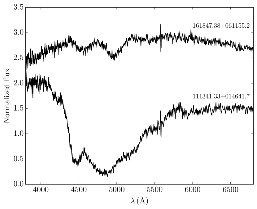
Figure 1: SDSS spectra of two unusual objects. Both spectra were smoothed and the spectrum of SDSS J161847.38+061155.2 was vertically shifted for clarity.

Table 2 lists the atmospheric parameters found following our fitting procedure (SDSS J161847.38+061155.2 is omitted from this table, see Section 3.1) and Figure 2 displays our fit to the spectroscopic data. Note that stars that were already analysed in Blouin et al. (2019) are not shown in Figure 2 as we assumed the same atmospheric parameters as those determined in that work (since our atmosphere code is unchanged). Most of the fits presented in Figure 2 are satisfactory. The shape and position of the Swan bands are generally well reproduced, even for the most extreme objects. In particular, our model matches the very deep absorption bands of SDSS J131146.93+292351.1 (GSC2U J131147.2+292348) much more closely than what was obtained with previous atmosphere codes (Carollo et al., 2003; Dufour et al., 2005). Moreover, we achieve a good fit for the most extreme DQpec white dwarfs of our sample (i.e., SDSS J124739.05+064604.6, SDSS J082955.77+183532.6, and SDSS J180302.57+232043, the three coolest star in Figure 2). Our models successfully reproduce the pronounced shift of the Swan bands for the high densities encountered at the photosphere of those objects ($\rho\approx 0.7\,$g cm^-3).

Table 2: Atmospheric parameters.

SDSS J	MWDD ID	$T_{\rm{eff}}$	$\log g$	$M$	$\log\,{\textrm{C/He}}$ a	Spectral
		(K)		($M_{\odot}$)	(by number)	type
–	GJ 2012	5210 (60)	7.907 (0.038)	0.514 (0.023)	$-$8.40	DQpec
–	LP 410$-$80	6360 (60)	7.993 (0.022)	0.569 (0.013)	$-$6.47	DQpec
–	Wolf 219	6515 (60)	7.974 (0.025)	0.558 (0.015)	$-$6.45	DQpec
–	LP 717$-$1	5375 (20)	7.906 (0.014)	0.514 (0.008)	$-$7.41	DQpec
–	GJ 1086	6080 (45)	8.146 (0.019)	0.663 (0.012)	$-$6.57	DQ
080455.42+171443.6	SDSS J080455.42+171443.6	5364 (33)	7.885 (0.038)	0.502 (0.022)	$-$7.19	DQpec
080558.84+072448.5	SDSS J080558.83+072447.8	5313 (42)	7.938 (0.046)	0.532 (0.027)	$-$7.09	DQpec
080843.15+464028.6	WD 0805+468	5427 (64)	7.913 (0.128)	0.518 (0.073)	$-$5.93	DQpec
082955.77+183532.6	[VV2010c] J082955.8+183532	4500 (24)	7.113 (0.787)	0.188 (0.320)	$-$7.76	DQpec
083618.13+243254.6	SDSS J083618.13+243254.6	5277 (54)	7.545 (0.174)	0.335 (0.072)	$-$7.39	DQpec
090208.40+201049.9	LP 426$-$49	5499 (110)	8.224 (0.021)	0.713 (0.014)	$-$5.37	DQ
090632.17+470235.8	SDSS J090632.17+470235.8	5561 (68)	8.238 (0.053)	0.722 (0.035)	$-$5.56	DQ
093537.00+002422.0	WD 0933+006	5539 (60)	8.144 (0.046)	0.660 (0.020)	$-$5.37	DQ
101141.53+284556.0	LP 315$-$42	4335 (165)	8.211 (0.085)	0.703 (0.057)	$-$6.80	DQpec
–	GJ 3614	4530 (215)	8.074 (0.124)	0.614 (0.078)	$-$7.20	DQpec
–	BD$-$18 3019B	5832 (86)	7.863 (0.052)	0.492 (0.029)	$-$6.74	DQpec
111341.33+014641.7	WD 1111+020	5961 (350)	8.709 (0.122)	1.027 (0.073)	$-$5.14	DQpec
112036.74+010629.3	SDSS J112036.74+010629.3	5893 (40)	7.253 (0.640)	0.320 (0.180)	$-$5.68	DQ
115933.10+130031.6	WD 1156+132	6410 (60)	8.011 (0.034)	0.580 (0.021)	$-$5.70	DQ
121037.44+140644.4	SDSS J121037.44+140644.4	5419 (23)	8.031 (0.174)	0.589 (0.107)	$-$7.00	DQpec
122545.88+470613.0	PSO J186.4406+47.1036	6294 (67)	7.924 (0.059)	0.528 (0.034)	$-$5.33	DQ
123313.48+082403.1	NLTT 31076	6316 (61)	7.970 (0.041)	0.555 (0.024)	$-$6.50	DQpec
124733.69+491524.7	SDSS J124733.70+491524.8	6092 (38)	7.897 (0.058)	0.512 (0.033)	$-$6.78	DQpec
124739.05+064604.6	PM J12476+0646	4545 (31)	7.929 (0.033)	0.526 (0.019)	$-$7.50	DQpec
131146.93+292351.1	WD 1309+296	5529 (40)	8.178 (0.018)	0.683 (0.012)	$-$5.27	DQ
133359.86+001654.8	WD 1331+005	5823 (71)	8.741 (0.038)	1.052 (0.022)	$-$5.13	DQpec
134118.68+022736.9	WD 1338+027	5785 (20)	8.098 (0.013)	0.632 (0.008)	$-$6.00	DQpec
145725.27+210747.3	SDSS J145725.27+210747.3	5841 (36)	7.962 (0.043)	0.548 (0.025)	$-$6.71	DQpec
161140.18+045127.0	USNO-B1.0 0948$-$00255808	5772 (30)	7.956 (0.026)	0.545 (0.015)	$-$6.92	DQpec
161414.12+172900.5	LP 444$-$33	5491 (101)	7.935 (0.059)	0.531 (0.034)	$-$6.73	DQpec
162635.58+154441.6	–	6379 (51)	8.082 (0.073)	0.623 (0.046)	$-$6.49	DQpec
180302.57+232043.3	SDSS J180302.57+232043.3	4400 (67)	7.694 (0.086)	0.400 (0.042)	$-$7.79	DQpec
183500.21+642917.0	SDSS J183500.21+642917.0	6754 (40)	7.951 (0.018)	0.545 (0.010)	$-$5.14	DQpec
223224.00$-$074434.3	WD 2229$-$080	6137 (44)	8.126 (0.028)	0.651 (0.018)	$-$5.56	DQpec
224153.46+043256.6	NLTT 54596	5903 (38)	7.920 (0.030)	0.524 (0.017)	$-$6.93	DQpec
225901.16+215843.9	–	6270 (49)	8.267 (0.180)	0.744 (0.119)	$-$5.22	DQpec
a Typically, the uncertainy on $\log\,{\textrm{C/He}}$ is 0.10 dex.

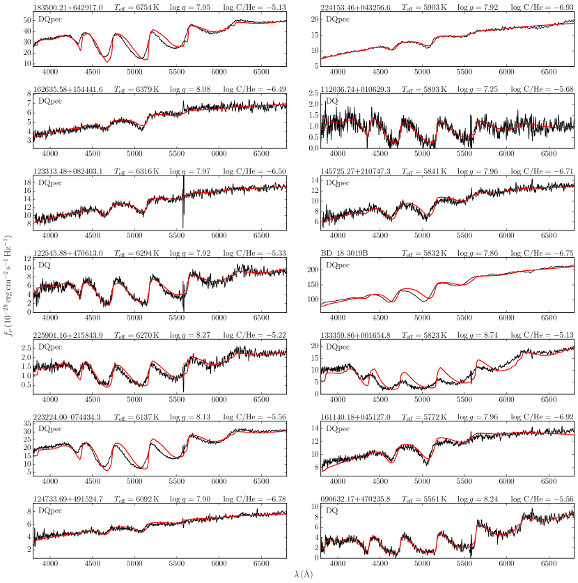
Figure 2: Spectroscopic fits of DQ/DQpec objects in our sample. Objects are shown in order of decreasing $T_{\rm eff}$. The DQ/DQpec classification is described in Section 4.2.

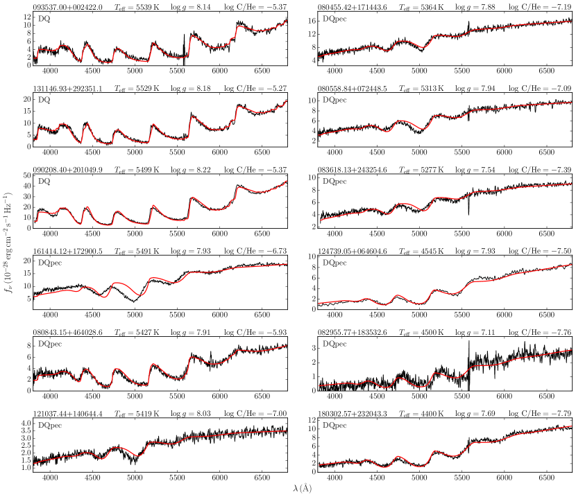
Figure 2 (cont.): Spectroscopic fits of DQ/DQpec objects in our sample. Objects are shown in order of decreasing $T_{\rm eff}$. The DQ/DQpec classification is described in Section 4.2.

3.1 Problematic objects

That being said, there is a rather diverse group of objects (BD$-$18 3019B, SDSS J111341.33+014641.7, SDSS J133359.86+001654.8, SDSS J161414.12+172900.5, SDSS J183500.21+642917.0, SDSS J223224.00$-$074434.3, SDSS J225901.16+215843.9) for which our models underestimate the amplitude of the Swan bands shift. The problem for those objects is that the effective temperature inferred from the photometric fit is too high to result in a photospheric density that would be high enough to sufficiently shift the Swan bands. The origin of the problem is unclear since these objects span a wide range of effective temperatures, carbon abundances and surface gravities. One possibility is that the empirically determined $\Delta T_{e}(\rm eV)=0.2\rho(\textrm{g\,cm}^{-3})$ shift, while valid for most objects, is too simplistic to properly capture the distortion of Swan bands under all physical conditions. Another possibility, also discussed in Blouin et al. (2019) in the context of other problematic objects, is that those stars may harbour a strong magnetic field that could affect their structures through the suppression of convection (Tremblay et al., 2015; Gentile Fusillo et al., 2018) and their radiative opacities through the magnetic distortion of the C₂ Swan bands (Liebert et al., 1978; Bues, 1991, 1999; Berdyugina et al., 2005, 2007). This scenario is compatible with the currently accessible spectropolarimetric data, since two out of those seven objects do show the presence of a magnetic field (SDSS J111341.33+014641.7 and SDSS J133359.86+001654.8, Schmidt et al., 2003). A serious challenge to this hypothesis, however, is the existence of highly magnetized DQ white dwarfs with undistorted Swan bands (GJ 1086, Berdyugina et al. 2007; WD 1235+422, Vornanen et al. 2013). It is unclear how a strong magnetic field could induce a shift in some stars and not in others.

Another peculiar object is SDSS J161847.38+061155.2. The SDSS spectrum of this object appears to show distorted Swan bands (Figure 1), but the effective temperature derived from the photometry (8700 K) is a few thousand degrees hotter than any other known DQpec white dwarf. A visual inspection of the SDSS and Pan–STARRS images has revealed that the field is not especially crowded so that the photometry does not seem to be contaminated by a blend of multiple objects. SDSS J161847.38+061155.2 could possibly be an unresolved binary, although this hypothesis is unlikely given the very high surface gravity of $\log g=8.6$ (and thus the small effective radius) obtained from the Gaia parallax.

4 The evolution of cool DQ/DQpec white dwarfs

4.1 The low–$T_{\rm eff}$ portion of the two DQ sequences

Figure 3 shows how the carbon abundance evolves with decreasing $T_{\rm{eff}}$ in DQ/DQpec white dwarfs. This figure clearly demonstrates that the two DQ sequences previously identified at $T_{\rm eff}\gtrsim 6500\,{\rm K}$ continue their courses down to the coolest DQpec white dwarfs. More precisely, a large fraction of DQpecs appears to correspond to the evolved versions of the “normal” DQs (i.e., normal-mass objects for which the atmospheric carbon originates from the dredge-up process) and a smaller fraction, the more massive and carbon-rich objects (e.g., SDSS J111341.33+014641.7 and SDSS J133359.86+001654.8), are likely descendants of Hot DQs. We note, however, that the origin of the normal-mass white dwarfs that lie above the main DQ sequence remains unclear.

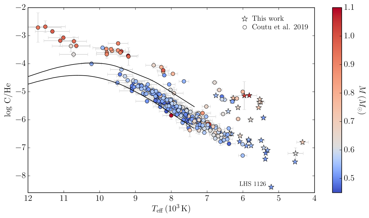
Figure 3: Carbon abundance as a function of effective temperature for the white dwarfs listed in Table 2 (stars) and for the DQ stars of Coutu et al. (2019, circles). The solid lines correspond to the evolutionary models of Fontaine & Brassard (2005) assuming $0.6\,M_{\odot}$ and $\log q({\rm He})=-3$ (top) or $\log q({\rm He})=-2$ (bottom). Objects with $M<0.45\,M_{\odot}$ were omitted from this figure as they are likely part of a binary system (Liebert et al., 2005; Rebassa-Mansergas et al., 2011).

These results, based on a detailed star-by-star analysis, imply that DQpec white dwarfs cannot all be descendants of Hot DQs as proposed by Koester & Kepler (2019). Note that their conclusion was reached based on the high surface gravities obtained from the Gaia parallaxes and SDSS photometry while assuming a fixed effective temperature and carbon abundance for all DQpec white dwarfs. In hindsight, the $T_{\rm eff}=7500\,{\rm K}$ and $\log\,{\rm C/He}=-5$ values assumed for all objects by Koester & Kepler (2019) were unrealistic, which explains why they found an average surface gravity of $\log g=8.625$.

Another argument of Koester & Kepler (2019) to support the scenario that DQpec white dwarfs are massive objects is that a high surface gravity can help increase the photospheric density and thus explain the density-driven shift of the Swan bands. However, our atmosphere models clearly demonstrate that this shift can happen in $\log g=8$ white dwarfs. A high photospheric density can be achieved as long as the effective temperature and the carbon abundance are low enough (Figure 4). A cool, carbon-poor atmosphere has fewer free electrons than a hot, carbon-rich atmosphere, which implies that He^- free–free (the main opacity in the atmosphere of those objects) is less prominent. This leads to a more transparent atmosphere and thus a photosphere that is located deeper in the star.

Figure 4: Density at the photosphere ($\tau_{R}=2/3$) of carbon-polluted white dwarfs as a function of $\log\,{\textrm{C/He}}$ , $T_{\rm{eff}}$ and $\log g$. The solid lines are for models with $\log g=8.0$ and the dashed lines are for $\log g=8.5$.

There is one object in Figure 3 that is an obvious outlier from the two DQ sequences. The very low $\log\,{\textrm{C/He}}$ value obtained for LHS 1126 in Blouin et al. (2019) implies that it is significantly below the main DQ sequence. However, the atmospheric parameters of this object remain highly uncertain as current models do not allow a satisfactory fit of its spectral energy distribution (SED). Many fits have been attempted, but none can explain all its SED from the ultraviolet to the mid-infrared (Bergeron et al., 1994; Wolff et al., 2002; Giammichele et al., 2012; Blouin et al., 2019). The challenge resides in simultaneously fitting its Ly$\alpha$ red wing, distorted Swan bands and infrared flux depletion.

4.2 The DQ$\rightarrow$DQpec transition

Another interesting aspect of the evolution of cool carbon-polluted white dwarfs is the question of where the DQ$\rightarrow$DQpec transition occurs. Figure 5 answers this question by indicating which objects are DQs and which ones are DQpecs in a $T_{\rm eff}-\log\,{\rm C/He}$ diagram. For this purpose, we needed a definition of the distinction between DQs and DQpecs. We thus performed two fits for each object, one in which the model grid includes a shift of the Swan bands and one in which the models assume that the Swan bands remain unperturbed by high-density effects. If the spectroscopic fit is significantly better when the shift is included, then the star is deemed a DQpec; otherwise, it is a DQ. As in the case of Figure 3, objects with $M<0.45\,M_{\odot}$ are ignored. Note also that many objects of the Coutu et al. (2019) sample are not shown in this figure as their low signal-to-noise spectra did not allow us to meaningfully distinguish between a DQ and a DQpec classification.

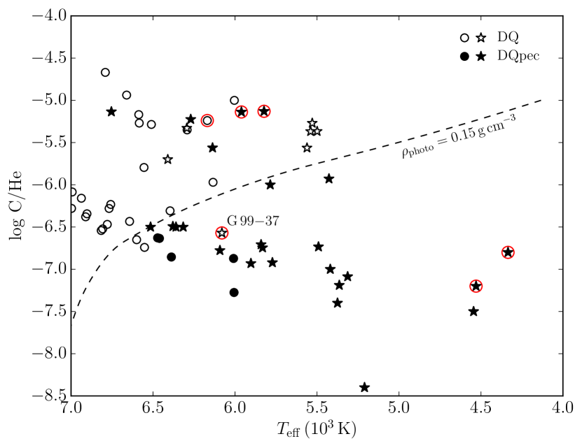
Figure 5: $T_{\rm eff}-\log\,{\rm C/He}$ diagram. The circles represent objects analysed in Coutu et al. (2019) and the stars are objects analysed in this work. The filled symbols correspond to DQpec white dwarfs, while the empty ones are DQs. Symbols encircled in red are known magnetic white dwarfs. The dashed line delimits the region where the photospheric density exceeds 0.15 g cm^-3 (assuming $\log g=8$), which marks the location of the DQ$\rightarrow$DQpec transition for most objects.

Figure 5 shows that the DQ$\rightarrow$DQpec transition occurs along a diagonal line in a $T_{\rm eff}-\log\,{\rm C/He}$ diagram. Given the density-driven nature of the distortion of the C₂ Swan bands and the relation between the photospheric density and $T_{\rm{eff}}$ and $\log\,{\textrm{C/He}}$ (Figure 4), this result is not surprising. As indicated in Figure 5, the distortion of the Swan bands (i.e., the DQpec phenomenon) starts to be detectable when the photospheric density (i.e., $\tau_{R}=2/3$) exceeds $\approx 0.15\,\textrm{g\,cm}^{-3}$.

There are however a few noteworthy exceptions to this pattern. SDSS J111341.33+014641.7, SDSS J133359.86+001654.8, SDSS J183500.21+642917.0, SDSS J223224.00-074434.3 and SDSS J225901.16+215843.9 are DQpec stars that have photospheric densities significantly below the $0.15\,\textrm{g\,cm}^{-3}$ threshold. Those five objects were already identified in Section 3.1 as objects for which our models underestimate the Swan bands shift. As explained above, it remains unclear whether this is due to our limited understanding of the behaviour of Swan bands under high-density conditions or to the presence of strong magnetic fields that alter the structure and opacities of those objects.

Another outlier is G 99$-$37 (GJ 1086), which shows undistorted Swan bands despite being surrounded by DQpec objects in Figure 5. This is probably explained by the presence of hydrogen in its atmosphere (G 99$-$37 has a CH $G$ band), which lowers its photospheric density. However, we note that this phenomenon is still not fully understood, as the hydrogen abundance required to match the CH $G$ band is insufficient to inhibit the distortion of the C₂ Swan bands (Blouin et al., 2019, Section 3.3.2).

5 Conclusions

A detailed star-by-star analysis of cool carbon-polluted white dwarfs was presented. We obtained good spectroscopic fits for the majority of objects in our sample, including cool DQs with very strong Swan bands and DQpec white dwarfs with strongly shifted bands. Our analysis reveals that cool DQ/DQpec stars follow the two evolutionary sequences previously identified at higher effective temperatures. A large fraction of objects appear to be white dwarfs that have dredged-up carbon from their cores and a smaller fraction could be descendants of Hot DQs. Our results imply that DQpecs represent the evolved versions of DQ white dwarfs no matter what the origin of carbon in those stars was.

For most objects, we find that the DQ$\rightarrow$DQpec transition occurs when the photospheric density reaches ${\approx 0.15\,\textrm{g\,cm}^{-3}}$. However, a few heavily polluted objects do not follow this trend and display distorted Swan bands even if their photospheric densities are significantly below $0.15\,\textrm{g\,cm}^{-3}$. This behaviour might be due to the presence of strong magnetic fields that can distort molecular bands. More efforts on both the observational and theoretical fronts are needed to clarify the nature of those objects. The number of DQpec white dwarfs for which spectropolarimetric data is available remains limited and the precise impact of strong magnetic fields on the C₂ Swan bands is unclear.

References

- Alam et al. (2015) Alam S., et al., 2015, ApJS, 219, 12
- Berdyugina et al. (2005) Berdyugina S. V., Braun P. A., Fluri D. M., Solanki S. K., 2005, A&A, 444, 947
- Berdyugina et al. (2007) Berdyugina S. V., Berdyugin A. V., Piirola V., 2007, Phys. Rev. Lett., 99, 091101
- Bergeron et al. (1994) Bergeron P., Ruiz M.-T., Leggett S. K., Saumon D., Wesemael F., 1994, ApJ, 423, 456
- Bergeron et al. (2001) Bergeron P., Leggett S. K., Ruiz M. T., 2001, ApJS, 133, 413
- Blouin et al. (2017) Blouin S., Kowalski P. M., Dufour P., 2017, ApJ, 848, 36
- Blouin et al. (2018a) Blouin S., Dufour P., Allard N. F., 2018a, ApJ, 863, 184
- Blouin et al. (2018b) Blouin S., Dufour P., Allard N. F., Kilic M., 2018b, ApJ, 867, 161
- Blouin et al. (2019) Blouin S., Dufour P., Thibeault C., Allard N. F., 2019, ApJ, 878, 63
- Brassard et al. (2007) Brassard P., Fontaine G., Dufour P., Bergeron P., 2007, in Napiwotzki R., Burleigh M. R., eds, Astronomical Society of the Pacific Conference Series Vol. 372, 15th European Workshop on White Dwarfs. p. 19
- Bues (1991) Bues I., 1991, in Vauclair G., Sion E., eds, NATO Advanced Science Institutes (ASI) Series C Vol. 336, 7th European Workshop on White Dwarfs. p. 285
- Bues (1999) Bues I., 1999, in Solheim S.-E., Meistas E. G., eds, Astronomical Society of the Pacific Conference Series Vol. 169, 11th European Workshop on White Dwarfs. p. 240
- Carollo et al. (2003) Carollo D., Koester D., Spagna A., Lattanzi M. G., Hodgkin S. T., 2003, A&A, 400, L13
- Chambers et al. (2016) Chambers K. C., et al., 2016, arXiv e-prints, p. arXiv:1612.05560
- Cheng et al. (2019) Cheng S., Cummings J. D., Ménard B., 2019, arXiv e-prints, p. arXiv:1905.12710
- Coutu et al. (2019) Coutu S., Dufour P., Bergeron P., Blouin S., Loranger E., Allard N. F., Dunlap B. H., 2019, arXiv e-prints, p. arXiv:1907.05932
- Dufour et al. (2005) Dufour P., Bergeron P., Fontaine G., 2005, ApJ, 627, 404
- Dufour et al. (2007) Dufour P., Liebert J., Fontaine G., Behara N., 2007, Nature, 450, 522
- Dufour et al. (2008) Dufour P., Fontaine G., Liebert J., Schmidt G. D., Behara N., 2008, ApJ, 683, 978
- Dufour et al. (2013) Dufour P., Vornanen T., Bergeron P., Fontaine Berdyugin A., 2013, in Krzesiński J., Stachowski G., Moskalik P., Bajan K., eds, Astronomical Society of the Pacific Conference Series Vol. 469, 18th European White Dwarf Workshop.. p. 167
- Dufour et al. (2017) Dufour P., Blouin S., Coutu S., Fortin-Archambault M., Thibeault C., Bergeron P., Fontaine G., 2017, in Tremblay P. E., Gaensicke B., Marsh T., eds, Astronomical Society of the Pacific Conference Series Vol. 509, 20th European White Dwarf Workshop. p. 3 (arXiv:1610.00986)
- Dunlap (2015) Dunlap B., 2015, PhD thesis, University of North Carolina at Chapel Hill Graduate School, Chapel Hill, NC, doi:10.17615/9y6e-cw21
- Dunlap & Clemens (2015) Dunlap B. H., Clemens J. C., 2015, in Dufour P., Bergeron P., Fontaine G., eds, Astronomical Society of the Pacific Conference Series Vol. 493, 19th European Workshop on White Dwarfs. p. 547
- Fontaine & Brassard (2005) Fontaine G., Brassard P., 2005, in Koester D., Moehler S., eds, Astronomical Society of the Pacific Conference Series Vol. 334, 14th European Workshop on White Dwarfs. p. 49
- Fontaine et al. (2001) Fontaine G., Brassard P., Bergeron P., 2001, PASP, 113, 409
- Gaia Collaboration et al. (2016) Gaia Collaboration et al., 2016, A&A, 595, A1
- Gaia Collaboration et al. (2018) Gaia Collaboration et al., 2018, A&A, 616, A1
- Gentile Fusillo et al. (2018) Gentile Fusillo N. P., Tremblay P.-E., Jordan S., Gänsicke B. T., Kalirai J. S., Cummings J., 2018, MNRAS, 473, 3693
- Giammichele et al. (2012) Giammichele N., Bergeron P., Dufour P., 2012, ApJS, 199, 29
- Hall & Maxwell (2008) Hall P. B., Maxwell A. J., 2008, ApJ, 678, 1292
- Jordan & Friedrich (2002) Jordan S., Friedrich S., 2002, A&A, 383, 519
- Kawka & Vennes (2012) Kawka A., Vennes S., 2012, MNRAS, 425, 1394
- Kepler et al. (2016) Kepler S. O., et al., 2016, MNRAS, 455, 3413
- Koester & Kepler (2019) Koester D., Kepler S. O., 2019, A&A, 628, A102
- Koester & Knist (2006) Koester D., Knist S., 2006, A&A, 454, 951
- Koester et al. (1982) Koester D., Weidemann V., Zeidler E. M., 1982, A&A, 116, 147
- Kowalski (2010) Kowalski P. M., 2010, A&A, 519, L8
- Kowalski & Saumon (2006) Kowalski P. M., Saumon D., 2006, ApJ, 651, L137
- Kowalski et al. (2007) Kowalski P. M., Mazevet S., Saumon D., Challacombe M., 2007, Phys. Rev. B, 76, 075112
- Kupka et al. (1999) Kupka F., Piskunov N., Ryabchikova T. A., Stempels H. C., Weiss W. W., 1999, A&AS, 138, 119
- Liebert et al. (1978) Liebert J., Angel J. R. P., Stockman H. S., Beaver E. A., 1978, ApJ, 225, 181
- Liebert et al. (2003) Liebert J., et al., 2003, AJ, 126, 2521
- Liebert et al. (2005) Liebert J., Bergeron P., Holberg J. B., 2005, ApJS, 156, 47
- Limoges et al. (2015) Limoges M. M., Bergeron P., Lépine S., 2015, ApJS, 219, 19
- Parigger et al. (2015) Parigger C. G., Woods A. C., Surmick D. M., Gautam G., Witte M. J., Hornkohl J. O., 2015, Spectrochimica Acta, 107, 132
- Pelletier et al. (1986) Pelletier C., Fontaine G., Wesemael F., Michaud G., Wegner G., 1986, ApJ, 307, 242
- Piskunov et al. (1995) Piskunov N. E., Kupka F., Ryabchikova T. A., Weiss W. W., Jeffery C. S., 1995, A&AS, 112, 525
- Rebassa-Mansergas et al. (2011) Rebassa-Mansergas A., Nebot Gómez-Morán A., Schreiber M. R., Girven J., Gänsicke B. T., 2011, MNRAS, 413, 1121
- Rohrmann (2018) Rohrmann R. D., 2018, MNRAS, 473, 457
- Ryabchikova et al. (2015) Ryabchikova T., Piskunov N., Kurucz R. L., Stempels H. C., Heiter U., Pakhomov Y., Barklem P. S., 2015, Physica Scripta, 90, 054005
- Schmidt et al. (1995) Schmidt G. D., Bergeron P., Fegley B., 1995, ApJ, 443, 274
- Schmidt et al. (1999) Schmidt G. D., Liebert J., Harris H. C., Dahn C. C., Leggett S. K., 1999, ApJ, 512, 916
- Schmidt et al. (2003) Schmidt G. D., et al., 2003, ApJ, 595, 1101
- Tremblay et al. (2015) Tremblay P.-E., Fontaine G., Freytag B., Steiner O., Ludwig H.-G., Steffen M., Wedemeyer S., Brassard P., 2015, ApJ, 812, 19
- Vornanen et al. (2013) Vornanen T., Berdyugina S. V., Berdyugin A., 2013, A&A, 557, A38
- Weidemann & Koester (1995) Weidemann V., Koester D., 1995, A&A, 297, 216
- Wolff et al. (2002) Wolff B., Koester D., Liebert J., 2002, A&A, 385, 995