Abstract

Refining one’s hypotheses in the light of data is a common scientific practice; however, the dependency on the data introduces selection bias and can lead to specious statistical analysis. An approach for addressing this is via conditioning on the selection procedure to account for how we have used the data to generate our hypotheses, and prevent information to be used again after selection. Many selective inference (a.k.a. post-selection inference) algorithms typically take this approach but will “over-condition” for sake of tractability. While this practice yields well calibrated statistic tests with controlled false positive rates (FPR), it can incur a major loss in power. In our work, we extend two recent proposals for selecting features using the Maximum Mean Discrepancy and Hilbert Schmidt Independence Criterion to condition on the minimal conditioning event. We show how recent advances in multiscale bootstrap makes conditioning on the minimal selection event possible and demonstrate our proposal over a range of synthetic and real world experiments. Our results show that our proposed test is indeed more powerful in most scenarios.

1 INTRODUCTION

Most statistical methods implicitly assume that parameters of the statistical investigation are fixed apriori; that is, the choice of model, hypothesis to test, and parameters to be estimated do not change before the data is inspected. Failure to satisfy this can lead to disturbing properties such as uncalibrated $p$-values (Simmons et al.,, 2011; Gelman and Loken,, 2013). The field of selective inference (SI) considers a modernised version of statistical analysis where we first explore the data and determine relevant parameters for our investigation. Then, SI aims to provide valid inference under the model chosen by the data (Fithian et al.,, 2014). In our work, we extend two algorithms that first select a set of features then perform hypothesis testing on each of the selected features to determine whether it is statistically significant.

One of the approaches in the field of SI is conditioning on how the data has been used during the initial selection phase (Fithian et al., (2014); Lee et al., (2016); Fithian et al., (2015)). This approach may be difficult to use since it requires an explicit characterisation of the selection procedure and the conditional distribution of the test statistic, both of which can be difficult to obtain. Fortunately, one of the key developments that has allowed many SI algorithms to be tractable is the polyhedral lemma (Lee et al.,, 2016; Tibshirani et al.,, 2016). Assume that the test statistic is normally distributed before the selection. The polyhedral lemma states that if the selection event can be written as a set of linear constraints, then its conditional post-selective distribution follows a truncated normal distribution (Lee et al.,, 2016, Theorem 5.2). This result has been successfully applied to non-parametric kernel methods for selecting informative features using the Hilbert Schmidt Independence Criterion (Yamada et al.,, 2018), and the Maximum Mean Discrepancy (Yamada et al.,, 2019), as well as multiple model comparison (Lim et al.,, 2019).

A subtlety with SI is that the power of selective hypothesis tests (i.e., tests with null hypothesis that is determined by data and so random) depends upon our choice of what to condition on. If we condition on too little, the test will have uncontrolled false positive rate. If we condition on too much, it can incur a loss of power (Fithian et al.,, 2014). This observation has driven research efforts to curate more powerful hypothesis tests that have higher “left-over” information. These proposals include randomising the data used during selection (Tian et al.,, 2018); a careful characterisation of how the data has been used during the selection process as there are different costs for variable selection and target formulation (Liu et al.,, 2018); and conditioning on the minimal set, i.e., condition only on what is necessary for the test to be valid but not more (Liu et al.,, 2018; Terada and Shimodaira,, 2019). The last idea forms the basis of what we propose in this work.

In the present work, we consider the problem of selecting a subset of informative features with selective inference. We study two related problem settings. In the first setting (Section 3), given two samples, the goal is to select a subset of features for which the marginal distributions (restricted to the selected subset) of the two underlying distributions significantly differ. In the second setting (Section 4), given a joint sample of covariate and response variables, the goal is to select a subset of covariate variables whose dependency on the response is statistically significant. While the selective tests of Yamada et al., (2019, 2018) are applicable to these problems, and have a tractable null distribution due to the use of the polyhedral lemma, these tests do not consider the minimal condition set, meaning that the tests may be overly conservative.

We generalize the tests of Yamada et al., (2019) and Yamada et al., (2018), for the two settings respectively, and propose tests that condition on the minimal conditioning set by using the selective multiscale bootstrap (Terada and Shimodaira,, 2017, 2019). For the second problem, we further propose a new estimator for the Hilbert Schmidt Independence Criterion (HSIC) that takes the form of an incomplete U-statistic. We show that the new estimator leads to a test that has higher power than the test of Yamada et al., (2018) which relies on the block estimator. In experiments (Section 5) on both synthetic and real problems, we show that the new tests have well-controlled false positive rate, and are more powerful than their respective original tests when the number of features is large, and the number of selected features is larger than one.

2 BACKGROUND

In this section, we review the Maximum Mean Discrepancy (MMD) and Hilbert Schmidt Independence Criterion (HSIC) which are used as our criteria to select features as well as briefly introduce the concept of multiscale bootstrap. In Section 3, we use MMD to select features that have significantly different marginal distributions and in Section 4, we use HSIC to select features which have a significant dependence on the response variable respectively.

Maximum Mean Discrepancy (MMD) For a distribution $P$ and a positive definite kernel $K$, the mean embedding of $P$ is defined as $\mu_{P}=\mathbb{E}_{x\sim P}[K(\cdot,x)]$ (Smola et al.,, 2007). The Maximum Mean Discrepancy (MMD) is a pseudo metric between two distributions $P$ and $Q$ and is defined as $\mathrm{MMD}(P,Q)=\|\mu_{P}-\mu_{Q}\|_{K}$, where $\|\cdot\|_{K}$ denotes the norma in the reproducing kernel Hilbert space (RKHS) associated with $K$. If $K$ is a characteristic kernel, then $\mathrm{MMD}^{2}(P,Q)=0\iff P=Q$ (Gretton et al.,, 2012). An example of a characteristic kernel is the Gaussian kernel. It can be shown that the squared MMD can be written equivalently as $\mathrm{MMD}^{2}(P,Q)=\mathbb{E}_{z,z^{\prime}\sim P\times Q}[h(z,z^{\prime})]$ where $z:=(x,y)$ and $h(z,z^{\prime}):=K(x,x^{\prime})+K(y,y^{\prime})-K(x^{\prime},y)-K(x,y^{\prime})$. Given samples $\bm{x}:=\{x_{i}\}_{i=1}^{n}$ and $\bm{y}:=\{y_{i}\}_{i=1}^{n}$ of size $n$ as i.i.d. draws from $P$ and $Q$ respectively, an unbiased estimator is the U-statistic $\widehat{\mathrm{MMD}}^{2}_{u}(\bm{x},\bm{y})=\frac{1}{n(n-1)}\sum_{i\neq j}h(z_{i},z_{j})$. In our work, we focus on a parametric bootstrap resampling procedure for multiscale bootstrap and thus we use estimators with normal asymptotic distributions such as the linear-time estimator $\widehat{\mathrm{MMD}}^{2}_{l}=\frac{2}{n}\sum_{i=1}^{n/2}h(z_{2i},z_{2i-1})$ (Gretton et al.,, 2012), and the incomplete U-statistic estimator (Blom,, 1976; Janson,, 1984) proposed by Yamada et al., (2019): $\widehat{\mathrm{MMD}}^{2}_{Inc}=\frac{1}{|\mathcal{D}_{n}|}\sum_{(i,j)\in\mathcal{D}_{n}}h(z_{i},z_{j})$ where $\mathcal{D}_{n}$ is random and sampled with replacement from $\{(i,j)\}_{i\neq j}$. Under weak assumptions, both $\widehat{\mathrm{MMD}}^{2}_{l}$ and $\widehat{\mathrm{MMD}}^{2}_{Inc}$ are asymptotically normal for both when $P=Q$ and $P\neq Q$ (Gretton et al.,, 2012; Yamada et al.,, 2019).

Hilbert Schmidt Independence Criterion (HSIC) Let $x\in\mathcal{X}$ and $y\in\mathcal{Y}$ be two random variables with joint distribution $P_{xy}$ and their respective marginals $P$ and $Q$. Let $K_{\mathcal{X}}$ and $K_{\mathcal{Y}}$ be two real-valued kernel functions defined on $\mathcal{X}\times\mathcal{X}$ and $\mathcal{Y}\times\mathcal{Y}$ respectively. The Hilbert Schmidt Independence Criterion (Gretton et al.,, 2005) is defined as the Hilbert-Schmidt norm of the covariance operator $\mathrm{HSIC}(P_{xy})=||\mu_{xy}-\mu_{P}\otimes\mu_{Q}||^{2}_{\mathrm{HS}}$ where $\otimes$ denotes the tensor product and $\mu_{xy}:=\mathbb{E}_{(x,y)\sim P_{xy}}[K_{\mathcal{X}}(x,\cdot)\otimes K_{\mathcal{Y}}(y,\cdot)]$. The norm $||\cdot||_{\mathrm{HS}}$ is induced by the inner product of the space of linear operators (that are Hilbert Schmidt). See Gretton et al., (2005, Section 2) for details. If the product kernel $K_{\mathcal{X}}K_{\mathcal{Y}}$ is characteristic on the joint domain $\mathcal{X}\times\mathcal{Y}$, then $\mathrm{HSIC}(P_{xy})=0\iff x\mathchoice{\mathrel{\hbox to0.0pt{$\displaystyle\perp$\hss}\mkern 2.0mu{\displaystyle\perp}}}{\mathrel{\hbox to0.0pt{$\textstyle\perp$\hss}\mkern 2.0mu{\textstyle\perp}}}{\mathrel{\hbox to0.0pt{$\scriptstyle\perp$\hss}\mkern 2.0mu{\scriptstyle\perp}}}{\mathrel{\hbox to0.0pt{$\scriptscriptstyle\perp$\hss}\mkern 2.0mu{\scriptscriptstyle\perp}}}y$ ($x$ and $y$ are independent) (Fukumizu et al.,, 2008, Theorem 3). An example of such a kernel can be constructed by letting $K_{\mathcal{X}}$ and $K_{\mathcal{Y}}$ be Gaussian kernels on $\mathcal{X}\subseteq\mathbb{R}^{d_{x}}$ and $\mathcal{Y}\subseteq\mathbb{R}^{d_{y}}$ respectively. Given $\bm{z}:=\{(x_{i},y_{i})\}_{i=1}^{n}$ consisting of $n$ i.i.d. samples from $P_{xy}$, an unbiased estimator can be computed as a U-statistic $\widehat{\mathrm{HSIC}}_{u}(\bm{z})=\frac{(n-4)!}{n!}\sum_{(i,j,q,r)\in\bm{i}^{n}_{4}}h(i,j,q,r)$ (Hoeffding,, 1992; Song et al.,, 2012) where $\bm{i}^{n}_{4}$ is the set of all $4$-tuples with each index occurring only once, $h(i,j,q,r)=\frac{1}{4!}\sum_{(s,t,u,v)}^{(i,j,q,r)}\bm{K}_{st}[\bm{L}_{st}+\bm{L}_{uv}-2\bm{L}_{su}]$ is the U-statistic kernel with the sum being over $4!$ quadruples $(s,t,u,v)$ as permutations of $(i,j,q,r)$, and $\bm{K,L}\in\mathbf{R}^{n,n}$ contain entries $\bm{K}_{ij}=K_{\mathcal{X}}(x_{i},x_{j})$, $\bm{L}_{ij}=K_{\mathcal{Y}}(y_{i},y_{j})$. If $x$ and $y$ are dependent then $\widehat{\mathrm{HSIC}}_{u}$ is asymptotically normally distributed (Song et al.,, 2012, Theorem 5). However, if they are independent then U-statistic is degenerate and the asymptotic distribution of $\widehat{\mathrm{HSIC}}_{u}$ deviates from normal (Gretton et al.,, 2008; Serfling,, 2009). For a given block size $B$, the block estimator of Zhang et al., (2018) is defined as $\widehat{\mathrm{HSIC}}_{Blo}(\bm{z})=\frac{B}{n}\sum_{i=1}^{\frac{n}{B}}\widehat{\mathrm{HSIC}}_{u}(\{z_{j}\}_{j=(i-1)B+1}^{iB})$. If $\lim_{n,B\rightarrow\infty}n/B=\infty$, it can be shown that the block estimator is normally distributed asymptotically even when $x$ is independent of $y$ (Zhang et al.,, 2018, Section 3.2).

Multiscale Bootstrap A procedure that calculates “approximately unbiased” $p$-values is called multiscale bootstrap proposed by Shimodaira, (2002); Shimodaira et al., (2004). It was initially proposed for a general statistical problem, called the problem of regions (Efron et al.,, 1998), where we want to compute asymptotically accurate $p$-values for the null hypothesis $H_{0}:\mu\in H$ where $H$ is represented by a region with $H\subseteq\mathbb{R}^{d}$ (called “hypothesis region”). Efron et al., (1996) studied this problem under the normal model $y\sim\mathcal{N}(\mu,I)$ and argued that the bootstrap probabilities $\textrm{BP}(H):=\mathbb{P}(y\in H)$ are biased frequentist confidence measures. Furthermore, they showed that geometric quantities play a crucial role and bias corrected $p$-values can be produced by using the pivotal quantity $\beta_{0}(y)-\beta_{1}\sim\mathcal{N}(0,1)$ where $\beta_{0}(y)$ is the signed distance from $y$ to $\partial H$ (i.e., the boundary surface of $H$), and $\beta_{1}$ is the mean curvature of $\partial H$. More specifically, a second-order asymptotically accurate $p$-value is expressed as $p(H|y):=\bar{\Phi}(\beta_{0}(y)-\beta_{1})$, i.e., $\forall\mu\in\partial H,\ \mathbb{P}(p(H|y)<\alpha)=\alpha+\mathcal{O}(n^{-1})$ (Efron et al.,, 1996; Shimodaira,, 2002). Note that $\Phi(\cdot)$ is the CDF of the standard normal distribution and $\bar{\Phi}(x):=1-\Phi(x)$. However, typically $\beta_{0}(y)$ and $\beta_{1}$ are hard to determine due to either the intractability of the space or the lack of an explicit formulation in the region. Multiscale bootstrap addresses this problem with additional computation and only requires the regions to be represented by a function that indicates if $y\in H$ or $y\notin H$.

Let $\mathcal{X}_{n}=\{x_{i}\}_{i=1}^{n}$ be a dataset of sample size $n$ with each element $x_{i}\in\mathbb{R}^{d}$. We assume that there is some transformation $f_{n}$ such that the observed value $f_{n}(\mathcal{X}_{n})$ follows a multivariate normal distribution, i.e., $y:=f_{n}(\mathcal{X}_{n})\sim\mathcal{N}(\mu,I)$. Typically, $f_{n}$ has a factor $\sqrt{n}$ for scaling the covariance. The main idea of multiscale bootstrap is, instead of $n$ elements, it resamples $n^{\prime}$ elements from $\mathcal{X}_{n}$ with replacement to generate $\mathcal{X}^{*}_{n^{\prime}}$, then $y^{*}:=f_{n}(\mathcal{X}^{*}_{n^{\prime}})\sim\mathcal{N}(y,\gamma^{2}I)$ with $\gamma^{2}=n/n^{\prime}$, from which we estimate the desired geometric quantities $\beta_{0}(y)$ and $\beta_{1}$ using the scaling law of bootstrap probabilities (Shimodaira,, 2002, 2014). It can be shown that the bootstrap probability of the region $H$ is expressed as $\textrm{BP}_{\gamma^{2}}(H):=\mathbb{P}(y^{*}\in H)\approx\bar{\Phi}(\gamma^{-1}\beta_{0}(y)+\gamma\beta_{1})$. Shimodaira, (2008, 2014) proposed the normalised bootstrap $z$-value as $\psi_{\gamma^{2}}(y|H):=\gamma\bar{\Phi}^{-1}(\textrm{BP}_{\gamma^{2}}(H))\approx\beta_{0}(y)+\gamma^{2}\beta_{1}$ from which $p$-values proposed by Efron et al., (1998), namely $p(H|y)=\bar{\Phi}(\beta_{0}(y)-\beta_{1})$, can be calculated when $\gamma^{2}=-1$, i.e., we have $\bar{\Phi}(\psi_{-1}(y|H))=\bar{\Phi}(\beta_{0}(y)-\beta_{1})=p(y|H)$. However, it is impossible to simulate the case where $\gamma^{2}=-1$. Multiscale bootstrap tackles this problem by using a number of different sample sizes $n^{\prime}\in\mathcal{M}\subset\mathbb{N}^{+}$. For each $n^{\prime}$, we run bootstrap resampling of $\mathcal{X}^{*}_{n^{\prime}}$ from $\mathcal{X}_{n}$ for calculating the normalised bootstrap $z$-value $\psi_{\gamma^{2}_{n^{\prime}}}(y|H))$ with $\gamma^{2}_{n^{\prime}}:=n/n^{\prime}$. The tuple $\{(\gamma^{2}_{n^{\prime}},\psi_{\gamma^{2}_{n^{\prime}}}(y|H))\}_{n^{\prime}\in\mathcal{M}}$ is used to fit a regression model $\varphi_{H}(\gamma^{2})$ which can then be extrapolated to $\varphi_{H}(-1)$. The regression model $\varphi_{H}(\cdot)$ can be used to calculate our $p$-values since $p(y|H)=\bar{\Phi}(\varphi_{H}(-1))$. See Shimodaira and Terada, (2019, Section 6.5) for several possibilities of regression models.

Selective Multiscale Bootstrap Multiscale bootstrap can be extended to the problem of selective inference, where the hypothesis is random and chosen from the data (Shimodaira and Terada,, 2019; Terada and Shimodaira,, 2017, 2019). In this problem, there is an additional region $S$ called the “selective region” that determines the null hypothesis we are going to test. If $y\in S$ then we test $H_{0}:y\in H$. However, if $y\not\in S$, we ignore $H$ and no decision is made. Terada and Shimodaira, (2017, 2019) proposed the following selective $p$-value

$$p(H|y,S)=\frac{\bar{\Phi}(\beta_{0}(y|H)-\beta_{1})}{\bar{\Phi}(\beta_{0}(y|H)-\beta_{1}+\beta_{0}(y|S))},$$

where $\beta_{1}$ is the mean curvature of $\partial H$, and $\beta_{0}(y|H)$ and $\beta_{0}(y|S)$ are the signed distances from $y$ to $\partial H$ and $\partial S$, respectively. Under certain assumptions, its null distribution is uniform over $(0,1)$ (Terada and Shimodaira,, 2017), i.e., we have

$$p(H|y,S)\,|\,y\in S,\,\mu\in\partial H\sim\mathcal{U}(0,1).$$

The calculation of $p(H|y,S)$ may again be non-trivial. The difficulty arises from the calculation of the signed distance $\beta_{0}(y|S)$ for the selective region $S$ but fortunately, we can apply the same idea as non-selective multiscale bootstrap as mentioned in previous subsection. In this case, another regression model $\varphi_{S}(\gamma^{2})$ is fitted with the bootstrap probabilities $\textrm{BP}_{\gamma^{2}}(S)$ for the region $S$. It can be seen that the signed distance $\beta_{0}(y|S)$ can then be obtained by extrapolating the model $\varphi_{S}(\gamma^{2})$ to $\gamma^{2}=0$. In other words, the selective $p$-value $p(H|y,S)$ can be calculated using two regression models $\varphi_{H}(\cdot)$ and $\varphi_{S}(\cdot)$ as follows,

$$p(H|y,S)=\frac{\bar{\Phi}(\varphi_{H}(-1))}{\bar{\Phi}(\varphi_{H}(-1)+\varphi_{S}(0))}.$$

Algorithm 1 Selective Multiscale Bootstrap

1:procedure SelectiveMS($\mathds{1}_{H},\mathds{1}_{S},\alpha,\,\bm{\mu},\bm{\Sigma}$)

2:     for $n^{\prime}\in\mathcal{M}$  do

3:         $\gamma^{2}_{n^{\prime}}\leftarrow\frac{n}{n^{\prime}}$

4:         Sample $\{\bm{y}^{*}_{i}\}^{B}_{i=1}\overset{i.i.d.}{\sim}\mathcal{N}(\bm{\mu},\,\gamma^{2}_{n^{\prime}}\bm{\Sigma})$

5:         $\textrm{BP}_{\gamma_{n^{\prime}}^{2}}(H)\leftarrow\sum^{B}_{i=1}\mathds{1}_{H}(\bm{y}^{*}_{i})/B$

6:         $\textrm{BP}_{\gamma_{n^{\prime}}^{2}}(S)\leftarrow\sum^{B}_{i=1}\mathds{1}_{S}(\bm{y}^{*}_{i})/B$

7:     end for

8:     Fit a model $\varphi_{H}(\gamma^{2})$ such that $\varphi_{H}(\gamma^{2})=\gamma\bar{\Phi}^{-1}(\textrm{BP}_{\gamma^{2}}(H))$.

9:     Fit a model $\varphi_{S}(\gamma^{2})$ such that $\varphi_{S}(\gamma^{2})=\gamma\bar{\Phi}^{-1}(\textrm{BP}_{\gamma^{2}}(S))$.

10:return $\bar{\Phi}(\varphi_{H}(-1))/\bar{\Phi}(\varphi_{H}(-1)+\varphi_{S}(0))$

11:end procedure

Algorithm 1 describes selective multiscale bootstrap algorithm where $\mathds{1}_{H}(y)$ is an indicator function: it is $1$ if $y\in H$, otherwise $0$.

3 SELECTIVE INFERENCE WITH MMD

In this section, we propose our first test. We are concerned with the following problem,

Problem 1.

Given two distributions $P$ and $Q$ with common support on $\mathcal{X}^{d}$, we have $n$ i.i.d.  samples denoted as $\bm{X}_{n}=[\bm{x}_{1},\dots,\bm{x}_{n}]^{\top}\in\mathcal{X}^{n\times d}$ with $\bm{x}\sim P$ and similarly for $\bm{Y}_{n}$ with $\bm{y}\sim Q$. Our goal is to find a set of features $\mathcal{S}$ such that for $i\in\mathcal{S}$, the marginal distributions of the $i$-th dimension of $\bm{x}$ and $\bm{y}$ (denoted as $P^{(i)}$ and $Q^{(i)}$) are significantly different, i.e., $P^{(i)}\neq Q^{(i)}$.

The problem and a solution were initially proposed by Yamada et al., (2019) based on the polyhedral lemma for post-selection inference. Their proposal mmdInf, which is referred to as PolyMMD in this paper, first selects a set of $k$ features $\mathcal{S}_{k}$ using MMD and then tests if each of the selected features’ marginal distributions are different. The latter part is performed by conditioning on selecting the whole set $\mathcal{S}_{k}$. This form of conditioning can be written equivalently as a set of linear constraints (Yamada et al.,, 2019, section 3.1) and as a result, it is possible to employ the polyhedral lemma and obtain a truncated normal as their asymptotic null distribution. However, we can relax the conditioning further. Notice that the goal is to test each feature $i\in\mathcal{S}_{k}$ separately. Thus, given a significance level $\alpha$, it is sufficient to require type-I error to be no larger than $\alpha$, conditioned only on $i\in\mathcal{S}_{k}$, rather than on the full set $\mathcal{S}_{k}$. Following Liu et al., (2018), we call this event the minimal conditioning set. While the selection event of PolyMMD can be written as a single polyhedron, the selection event $i\in\mathcal{S}_{k}$ is more complicated.

In this section, we propose MultiMMD a more powerful variant of PolyMMD by conditioning on the minimal conditioning set. We show how the statistical test can be performed using multiscale bootstrap. Although for the remainder of the section we focus on the incomplete estimator $\widehat{\mathrm{MMD}}^{2}_{Inc}$, a similar procedure can be applied to the block estimator $\widehat{\mathrm{MMD}}^{2}_{Blo}$ and the linear time estimator $\widehat{\mathrm{MMD}}^{2}_{l}$.

3.1 Proposal: MultiMMD

From the index set of all features $\mathcal{I}$, MultiMMD finds a subset of $k$ features, denoted by $\mathcal{S}_{k}\subseteq\mathcal{I}$, that differentiates samples from $P$ and $Q$. The $k$ features are selected as the $k$ dimensions with the highest scores measured by an estimator of MMD. More precisely, we have $\mathcal{S}_{k}=\mathcal{S}_{k-1}\cup\{\arg\max_{i\in\mathcal{I}\setminus\mathcal{S}_{k-1}}\widehat{\mathrm{MMD}}^{2}_{Inc}(\bm{X}_{n}^{(i)},\bm{Y}_{n}^{(i)})\}$ where $\bm{X}_{n}^{(i)}=[\bm{x}^{(i)}_{1},\dots,\bm{x}^{(i)}_{n}]^{\top}$ and $\bm{x}^{(i)}$ is the $i$-th dimension of the random variable $\bm{x}$ (and similarly for $\bm{Y}_{n}^{(i)}$) and $\mathcal{S}_{0}=\emptyset$.

The selection procedure mentioned above for MultiMMD is the same as PolyMMD, but the statistical test we perform is different. For each selected feature $i\in\mathcal{S}_{k}$, the hypothesis test we execute is

$$H_{0,i}:\mathrm{MMD}^{2}(P^{(i)},Q^{(i)})=0\ |\ i\in\mathcal{S}_{k}\text{ is selected},$$

$$H_{1,i}:\mathrm{MMD}^{2}(P^{(i)},Q^{(i)})>0\ |\ i\in\mathcal{S}_{k}\text{ is selected}.$$

In contrast to PolyMMD, when testing $H_{0,i}$ for some $i\in\mathcal{S}_{k}$, all the other selected variables in $\mathcal{S}_{k}\setminus\{i\}$ are not considered for conditioning. The justification of why tests that condition on the minimal conditioning set is more powerful can be found in Fithian et al., (2014). The main idea is that the monotonicity of the selective type I error, defined as $\mathbb{P}(\mathrm{Reject\,}H_{0,i}\leq\alpha\,|\,H_{0,i},i\in\mathcal{S}_{k})$, suggests that we will lose power when we move from coarse selection variables to finer selection variables (Fithian et al.,, 2014, Proposition 3).

Multiscale bootstrap’s flexibility in representing hypothesis and selective regions with indicator functions makes it a suitable candidate to calculate $p$-values. It requires us to define a set $\mathcal{M}$ with each of its members $n^{\prime}\in\mathcal{M}$ specifying the number of elements to be resampled from $\bm{X}_{n}$ and $\bm{Y}_{n}$ (denoted as $\bm{X}_{n^{\prime}}$ and $\bm{Y}_{n^{\prime}})$. We generate bootstrap replicates of statistic $\hat{\bm{T}}_{n}(\bm{X}_{n^{\prime}},\bm{Y}_{n^{\prime}}):=\sqrt{l_{n}}[\widehat{\mathrm{MMD}}^{2}_{Inc}(\bm{X}_{n^{\prime}}^{(1)},\bm{Y}_{n^{\prime}}^{(1)}),\dots,\widehat{\mathrm{MMD}}^{2}_{Inc}(\bm{X}_{n^{\prime}}^{(d)},\bm{Y}_{n^{\prime}}^{(d)})]^{\top}$ where $l_{n}=|\mathcal{D}_{n}|$ is the denominator used for $\widehat{\mathrm{MMD}}^{2}_{Inc}(\bm{X}_{n}^{(i)},\bm{Y}_{n}^{(i)})$. For each $n^{\prime}\in\mathcal{M}$, the statistic is computed $B$ times and the bootstrap probability $\textrm{BP}_{\gamma^{2}}(\cdot)$ of the hypothesis region $H$ (and selective region $S$) is the average number of the $B$ samples that falls within $H$ (and $S$). As a result, we require a sampler for $\hat{\bm{T}}_{n}(\bm{X}_{n^{\prime}},\bm{Y}_{n^{\prime}})$ for all $n^{\prime}\in\mathcal{M}$ and a function that describes whether the statistic falls within the regions $H$ and $S$. Finally, two linear regression models are fitted: one for $H$ and one for $S$ denoted as $\varphi_{H}(\cdot)$ and $\varphi_{S}(\cdot)$ respectively. Assuming that the boundary surfaces can be represented by a polynomial of degree 3, then the existing theory recommends a linear model (Shimodaira,, 2008, Section 5.4). The model’s predictor variable is the ratio $\gamma^{2}_{n^{\prime}}:=\frac{n}{n^{\prime}}$ and its response variable is $\gamma_{n^{\prime}}\bar{\Phi}^{-1}(\textrm{BP}_{\gamma^{2}_{n^{\prime}}}(\cdot))=\beta_{0}+\gamma^{2}_{n^{\prime}}\beta_{1}$ where $\beta_{0}$ is the signed distance from our statistic to the boundary of the region and $\beta_{1}$ the mean curvature at the boundary.

Algorithm 2 MultiMMD($\bm{X}_{n},\,\bm{Y}_{n},k,\,\mathcal{M}$): Selective $p$-values for the null hypothesis $H_{0,i}:\mathrm{MMD}^{2}(P^{(i)},Q^{(i)})=0\ |\ i\in\mathcal{S}_{k}\text{ is selected}$.

1:$\hat{\bm{T}}_{n}(\bm{X}_{n},\bm{Y}_{n}),\hat{\bm{\Sigma}}\leftarrow$EstimateParam($\bm{X}_{n}$, $\bm{Y}_{n}$)

2:$\mathcal{S}_{k}\leftarrow$ the indexes of $k$ largest values of $\{\widehat{\mathrm{MMD}}^{2}(\bm{X}_{n}^{(i)},\bm{Y}_{n}^{(i)})\}_{i\in\mathcal{I}}$

3:for $i\in\mathcal{S}_{k}$ do

4:     for $n^{\prime}\in\mathcal{M}$ do

5:         $\gamma^{2}_{n^{\prime}}\leftarrow\frac{n}{n^{\prime}}$

6:         Sample $\{\bm{y}^{*}_{i}\}^{B}_{i=1}\overset{i.i.d.}{\sim}\mathcal{N}(\hat{\bm{T}}_{n}(\bm{X}_{n},\bm{Y}_{n}),\,\gamma^{2}_{n^{\prime}}\hat{\bm{\Sigma}})$

7:         $\textrm{BP}_{\gamma_{n^{\prime}}^{2}}(S)\leftarrow\sum^{B}_{i=1}\mathds{1}^{(i)}_{S}(\bm{y}^{*}_{i})/B$

8:     end for

9:     Fit a linear model $\varphi_{S}(\gamma^{2})$ such that $\varphi_{S}(\gamma^{2})=\gamma\bar{\Phi}^{-1}(\textrm{BP}_{\gamma^{2}}(S))$.

10:     $\hat{\beta}_{0}^{(i)}\leftarrow\hat{\sigma}_{i}^{-1}\sqrt{l_{n}}\widehat{\mathrm{MMD}}^{2}_{Inc}(\bm{X}_{n}^{(i)},\bm{Y}_{n}^{(i)})$

11:     $p_{i}\leftarrow\bar{\Phi}(\hat{\beta}_{0}^{(i)})/\bar{\Phi}(\hat{\beta}_{0}^{(i)}+\varphi_{S}(0))$

12:end for

13:return $\{p_{i}\}_{i=0}^{k}$ and $\mathcal{S}_{k}$

We begin by describing how to obtain samples of $\hat{\bm{T}}_{n}(\bm{X}_{n^{\prime}},\bm{Y}_{n^{\prime}})$ for all $n^{\prime}\in\mathcal{M}$. Suppose that the bootstrap resamples can be represented using the distribution $\mathcal{N}(\hat{\bm{T}}_{n}(\bm{X}_{n},\bm{Y}_{n}),\hat{\bm{\Sigma}})$ where $\hat{\bm{\Sigma}}$ be the sample covariance of $\widehat{\mathrm{MMD}}^{2}_{Inc}$, i.e., $\hat{\bm{\Sigma}}:=\frac{1}{l_{n}-1}\sum_{(i,j)\in\mathcal{D}_{n}}[\bm{h}(\bm{z}_{i},\bm{z}_{j})-\overline{\bm{h}}][\bm{h}(\bm{z}_{i},\bm{z}_{j})-\overline{\bm{h}}]^{\top}$ where (recall that $h(\cdot,\cdot)$ is the U-statistic kernel) $\bm{h}(\bm{z}_{i},\bm{z}_{j}):=[h(\bm{z}^{(1)}_{i},\bm{z}^{(1)}_{j}),\ldots,h(\bm{z}^{(d)}_{i},\bm{z}^{(d)}_{j})]^{\top}\in\mathbb{R}^{d}$ and $\overline{\bm{h}}:=\frac{1}{l_{n}}\sum_{(i,j)\in\mathcal{D}_{n}}\bm{h}(\bm{z}_{i},\bm{z}_{j})$. The choice of normal distribution is justified as $\hat{\bm{T}}_{n}(\bm{X}_{n},\bm{Y}_{n})$ tends to be normally distributed as $n\rightarrow\infty$ (Yamada et al.,, 2019, Theorem 5). In order to replicate samples of $\hat{\bm{T}}_{n}(\bm{X}_{n^{\prime}},\bm{Y}_{n^{\prime}})$, notice that its asymptotic distribution is $\hat{\bm{T}}_{n}(\bm{X}_{n^{\prime}},\bm{Y}_{n^{\prime}})\sim\mathcal{N}(\hat{\bm{T}}_{n}(\bm{X}_{n},\bm{Y}_{n}),\frac{l_{n}}{l_{n^{\prime}}}\hat{\bm{\Sigma}})$. For each $n^{\prime}$, instead of resampling $n^{\prime}$ elements from $\bm{X}_{n}$ and $\bm{Y}_{n}$ for calculating $\hat{\bm{T}}_{n}(\bm{X}_{n^{\prime}},\bm{Y}_{n^{\prime}})$ $B$ times, we generated $B$ replicates directly from $\mathcal{N}(\hat{\bm{T}}_{n}(\bm{X}_{n},\bm{Y}_{n}),\frac{l_{n}}{l_{n^{\prime}}}\hat{\bm{\Sigma}})$ which is then used to calculate bootstrap probabilities. The former is an $\mathcal{O}(n^{\prime}B)$ process while the latter is $\mathcal{O}(B)$. In practice, the $B$ replicates are sampled from $\mathcal{N}(\hat{\bm{T}}_{n}(\bm{X}_{n},\bm{Y}_{n}),\frac{n}{n^{\prime}}\hat{\bm{\Sigma}})$ instead because we let $l_{n}$ and $l_{n^{\prime}}$ be the typical choice of $l_{n}=rn$ and $l_{n^{\prime}}=rn^{\prime}$ where $r$ is fixed apriori with $0<r<\infty$. The choice of $r$ affects the distribution of $\hat{\bm{T}}_{n}(\cdot,\cdot)$ (Yamada et al.,, 2019, section 4). When $r$ is high, its asymptotic distribution tends towards its complete counterpart (i.e., infinite sums of weighted chi-squared variables). But when $r$ is small, it is normally distributed.

For each $n^{\prime}$, the $B$ replicates are used to calculate bootstrap probabilities for both the hypothesis region $\textrm{BP}_{\frac{n}{n^{\prime}}}(H)$ and the selective region $\textrm{BP}_{\frac{n}{n^{\prime}}}(S)$. Note that the hypothesis $H_{0,i}$ can be written as the region $H=\{y\in\mathbb{R}^{d}:y^{(i)}\leq 0\}$ which has a flat boundary. This means that the curvature is $\beta_{1}=0$ and multiscale bootstrap is not needed for the hypothesis region $H$. In fact, the signed distance for testing $i\in\mathcal{S}_{k}$ is $\hat{\beta}^{(i)}_{0}=\hat{\sigma}^{-1}_{i}\sqrt{l_{n}}\widehat{\mathrm{MMD}}^{2}_{Inc}(\bm{X}_{n}^{(i)},\bm{Y}_{n}^{(i)})$ where $\hat{\sigma}^{2}_{i}$ is the $i$th diagonal element of $\hat{\bm{\Sigma}}$. We have $\varphi_{H}(\gamma^{2})=\hat{\beta}^{(i)}_{0}$ as a constant function.

However, it is not as easy for the selective region $S$ which requires the application of multiscale bootstrap. $S$ is represented by an indicator function $\mathds{1}_{S}^{(i)}(\bm{y}^{*})=\begin{cases}1&\text{if }i\in\mathcal{S}^{*}_{k}\\ 0&\text{if }i\notin\mathcal{S}^{*}_{k}\end{cases}$ where $\mathcal{S}^{*}_{k}$ is the selected set of $k$ features where our selection algorithm is applied to $\bm{y}^{*}$. Let $\gamma_{n^{\prime}}^{2}=\frac{n}{n^{\prime}}$ then, the bootstrap probability is given by $\textrm{BP}_{\gamma_{n^{\prime}}^{2}}(S)=\sum^{B}_{i=1}\mathds{1}^{(i)}_{S}(\bm{y}^{*}_{i})/B$ where $\{\bm{y}^{*}_{i}\}^{B}_{i=1}\overset{i.i.d.}{\sim}\mathcal{N}(\hat{\bm{T}}_{n}(\bm{X}_{n},\bm{Y}_{n}),\,\gamma^{2}_{n^{\prime}}\hat{\bm{\Sigma}})$. For a given $\mathcal{M}=\{n^{\prime}\}$, we have $|\mathcal{M}|$ pairs of predictor and response $\{(\gamma^{2}_{n^{\prime}},\gamma_{n^{\prime}}\bar{\Phi}^{-1}(\textrm{BP}_{\gamma^{2}_{n^{\prime}}}(S)))\}_{n^{\prime}\in\mathcal{M}}$ that is used to fit a linear model $\varphi_{S}(\gamma^{2})$. We define $\mathcal{M}$ to be the set of numbers equally spaced between $0.5n$ to $2n$ in log space with $|\mathcal{M}|=10$. The function $\varphi_{S}(\gamma^{2})$ can be used to extrapolate to $\gamma^{2}=0$ to obtain the signed distance from our statistic to the boundary of $S$. Then, our selective $p$-value for feature $i\in\mathcal{S}_{k}$ is given by

$$p_{i}=\bar{\Phi}(\hat{\beta}_{0}^{(i)})/\bar{\Phi}(\hat{\beta}_{0}^{(i)}+\varphi_{S}(0)).$$

We reject $H_{0,i}$ if $p_{i}<\alpha$. The algorithm is described in Algorithm 2.

4 SELECTIVE INFERENCE WITH HSIC

We consider the problem studied in Yamada et al., (2018)

Problem 2.

Given $n$ samples from the joint distribution $\{(\bm{x}_{i},\bm{y}_{i})\}^{n}_{i=1}\overset{i.i.d.}{\sim}P_{\bm{x}\bm{y}}$ on the domain $\mathcal{X}^{d}\times\mathcal{Y}$, our goal is to find a subset $\mathcal{S}$ of features of $\bm{x}$ such that for each $i\in\mathcal{S}$ there is statistically significant dependency between the feature $\bm{x}^{(i)}$ and response $\bm{y}$.

The goal is to decide if there is some dependence between the marginal distribution $\bm{x}^{(i)}$ and the response $\bm{y}$. Whereas in MultiMMD, it compares if the difference between the marginal distributions of $\bm{x}^{(i)}$ and $\bm{y}^{(i)}$ is zero, i.e., if $\mathrm{MMD}^{2}(\bm{x}^{(i)},\bm{y}^{(i)})=0$. In Yamada et al., (2018), a solution was proposed for Problem 2 using HSIC to measure the dependency between the two between $\bm{x}^{(i)}$ and $\bm{y}$ which we call “PolyHSIC” (previously called hsicInf). It begins with first selecting $k$ features with the highest HSIC scores and then a test is performed for each feature. But the conditioning is not minimal and suffers from a loss in power.

In this section, we propose a new estimator based on the incomplete U-statistic estimator for HSIC and analyse its asymptotic distribution. We then extend PolyHSIC to “MultiHSIC”. The new proposal conditions on the minimal conditioning set which is made possible with the multiscale bootstrap. Although our procedure allows the use of the HSIC block estimator (Zhang et al.,, 2018), we observe that the convergence of the estimator to the target normal distribution highly depends on the block size and in turn the number of blocks, which can be challenging to set correctly. As a result, the false rejection rate of the test can be difficult to control. See Appendix C.2 for a numerical simulation that illustrates this problem, and Zaremba et al., (2013, page 5) for a discussion on a similar issue in the block estimator for MMD.

4.1 Incomplete HSIC

We propose an estimator of HSIC that behaves as desired with the type I error at size $\alpha$ (unlike the block estimator) when used in conjunction with multiscale bootstrap. It based on the incomplete U-statistic estimator (Blom,, 1976; Janson,, 1984) defined as

$$\widehat{\mathrm{HSIC}}_{Inc}(\bm{z})=\frac{1}{l}\sum_{(i,j,q,r)\in\mathcal{D}}h(i,j,q,r)$$

where $\bm{z}=[z_{1},\dots,z_{n}]$ of $n$ i.i.d. draws from $z:=(x,y)\sim P_{xy}$, $l=|\mathcal{D}|$, and $\mathcal{D}$ is the design of the matrix and for $\widehat{\mathrm{HSIC}}_{Inc}$ it is constructed randomly by sampling $l$ terms with replacement from $\bm{i}^{n}_{4}$.

The asymptotic distribution of $\mathrm{\widehat{HSIC}}_{Blo}$ is normal in both cases when $y$ and $x$ are independent and dependent (Zhang et al.,, 2018, section 3.2). As shown in Corollary 1, it also follows that $\widehat{\mathrm{HSIC}}_{\text{Inc}}$ is asymptotically normal regardless of the presence of the dependency between $x$ and $y$ (in Appendix B, we empirically validate this claim).

Corollary 1 (Asymptotic Distribution of $\widehat{\mathrm{HSIC}}_{\text{Inc}}$).

Assume that $\lim_{n,l\rightarrow\infty}n^{-2}l=0$ and $0<\lim_{n,l\rightarrow\infty}n^{-1}l=\lambda<\infty$,

• If $X\mathchoice{\mathrel{\hbox to0.0pt{$\displaystyle\perp$\hss}\mkern 2.0mu{\displaystyle\perp}}}{\mathrel{\hbox to0.0pt{$\textstyle\perp$\hss}\mkern 2.0mu{\textstyle\perp}}}{\mathrel{\hbox to0.0pt{$\scriptstyle\perp$\hss}\mkern 2.0mu{\scriptstyle\perp}}}{\mathrel{\hbox to0.0pt{$\scriptscriptstyle\perp$\hss}\mkern 2.0mu{\scriptscriptstyle\perp}}}Y$, then $l^{\frac{1}{2}}\widehat{\mathrm{HSIC}}_{\text{Inc}}(\bm{z})\overset{d}{\rightarrow}\mathcal{N}(0,\sigma^{2})$,

• If $X\not\!\perp\!\!\!\perp Y$, then $l^{\frac{1}{2}}(\widehat{\mathrm{HSIC}}_{\text{Inc}}(\bm{z})-\mathrm{HSIC}(P_{xy}))\overset{d}{\rightarrow}\mathcal{N}(0,\lambda\sigma_{u}^{2}+\sigma^{2})$,

where $\sigma^{2}=\mathrm{Var}[h(i,j,q,r)]$ and $\sigma_{u}^{2}$ is the variance of the complete U-statistic counterpart, see Song et al., (2012, Theorem 5).

A measure of its performance is asymptotic relative efficiency ($\mathrm{ARE}$) (Lee,, 2019) of the incomplete estimator with respect its complete counterpart

$$\mathrm{ARE} =\lim_{n\rightarrow\infty}\mathrm{Var}(\widehat{\mathrm{HSIC}}_{Inc})/\mathrm{Var}(\widehat{\mathrm{HSIC}}_{u})$$

$$=\lim_{n\rightarrow\infty}\frac{(\lambda\sigma_{u}^{2}+\sigma^{2})/l}{\sigma_{u}^{2}/n}=1+\frac{\sigma^{2}}{r\sigma_{u}^{2}},$$

where a common choice of $l$ is chosen to be $rn$ for some $r>0$. This means that for large $r$ the incomplete estimator is asymptotically efficient and dependent on the ratio $\frac{\sigma^{2}}{\sigma_{u}^{2}}$ i.e., if we set $r$ to be big, we have $\mathrm{ARE}\approx 1$. A similar analysis can be performed for the incomplete estimator for the MMD which suggests we should take $r$ to be very high but it would violate our assumption that $\lim_{n\rightarrow\infty}n^{-1}l<\infty$ so the estimator will deviate from normal.

4.2 Proposal: MultiHSIC

In this section, we outline MultiHSIC as a more powerful method for variable selection by considering the minimal conditioning set. The algorithm begins by selecting $k$ features with the $k$ largest $\widehat{\mathrm{HSIC}}$ scores and then performing a test after selection. We have

$$H_{0,i}:\textrm{HSIC}(P_{\bm{x}^{(i)}\bm{y}})=0\ |\ i\in\mathcal{S}_{k}\text{ is selected},$$

$$H_{1,i}:\textrm{HSIC}(P_{\bm{x}^{(i)}\bm{y}})>0\ |\ i\in\mathcal{S}_{k}\text{ is selected},$$

where $P_{\bm{x}^{(i)}\bm{y}}$ is defined as the joint distribution between $\bm{x}^{(i)}$ and $\bm{y}$. Define $\bm{Z}^{(i)}=[\bm{z}^{(i)}_{1},\dots,\bm{z}^{(i)}_{n}]$ and $\bm{z}^{(i)}:=(x^{(i)},y)$. Let $\mathcal{S}_{k}=\mathcal{S}_{k-1}\cup\{\arg\max_{i\in\mathcal{D}\setminus\mathcal{S}_{k-1}}\widehat{\mathrm{HSIC}}_{Inc}(\bm{Z}^{(i)})\}$ and $\mathcal{S}_{0}=\emptyset$.

Related Work: Slim et al., (2019) proposed a class of kernel based statistics for selecting variables which can later be used for hypothesis testing. Their selective inference algorithm includes a sampler for simulating the null hypothesis. While we have focused on feature selection algorithms that condition on selection events to solve Problem 2, there is another branch of selective inference procedures based on the knockoff filter (Barber et al.,, 2019) which has been extended to the high dimensional setting (Candes et al.,, 2018). Their framework is similar in the sense that they too first select promising features and then provide selective guarantee on the inference made on the selected variables. However, their guarantees are based on generating convincing knock-offs variables such that the joint distribution is invariant between swaps of the variables and its knockoffs, which can be hard (Lu et al.,, 2018; Romano et al.,, 2019). These proposals control false discovery rate (Benjamini and Hochberg,, 1995).

5 EXPERIMENTS

In this section, we demonstrate our proposed method for both toy and real world datasets. The performance of our algorithm is measured by true positive rate (TPR) and false positive rate (FPR) which can be thought of as power and type-I error. TPR is defined to be the portion of true selected features that are correctly declared as such and FPR quantifies the portion of selected false features that are declared as incorrectly significant (see definitions in Section A). It is desirable to have high true positive rate and false positive rate to be controlled at $\alpha$ (it is not desirable for this to be below $\alpha$ or above $\alpha$) since the threshold is chosen to be such that the type-I error is size $\alpha$. Unless specified otherwise, we use the Gaussian kernel with its bandwidth chosen with the median heuristic.

Our first experiment considers several synthetic problems to evaluate our proposal and verify that our test controls FPR at nominal levels. For MMD, we use the mean shift problem varying both $n$ and $d$ and, for HSIC, we consider the logistic problem. Then, we proceed to using several real world data-sets which have been augmented with artificial and independent features. We consider the original preprocessed features as “true” features which allows us to calculate TPR and FPR. For MMD, we split the data-set into two sets for two different classes and the goal here is to “rediscover” the original features (with a minimal number of artificially added and uninformative features). And for HSIC, the data-set is split into the predictor variables (with some fakes) and the response variable, the goal here is to find the original predictors. For our final experiment, we consider the problem of anomalous dataset detection where $d$ is small (and so $k$ is small too). In this scenario, our algorithm only has incremental increase in power. Additional experiments can be found in the Appendix E. Code for reproducing our results is available online: https://github.com/jenninglim/multiscale-features.

5.1 Toy Problems

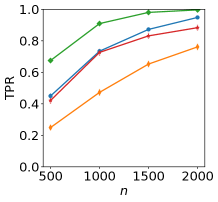
(a)

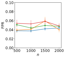
(b)

Figure 1: Mean shift experiment as $n$ increases. Results are shown for $\mathrm{\widehat{MMD}}^{2}_{l}$ and $\mathrm{\widehat{MMD}}^{2}_{Inc}$.

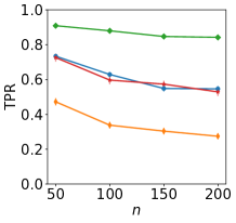
(a)

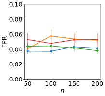
(b)

Figure 2: Mean shift experiment as $d$ increases. Results are shown for $\mathrm{\widehat{MMD}}^{2}_{l}$ and $\mathrm{\widehat{MMD}}^{2}_{Inc}$.

The aim of these synthetic experiment is to evaluate our proposals, MultiMMD and MultiHSIC, against previously proposed methods and empirically verify the theoretical guarantees. The TPR and FPR are averaged over $100$ trials, $k=30$ and $\alpha=0.05$. We consider the three scenarios.

MMD: Mean Shift with varying $n$ $(d=50)$. We are given $n$ samples from $P=\mathcal{N}(\bm{0},\bm{I})$ and $Q=\mathcal{N}(\bm{\mu},\bm{I})$ where $\mu=[\bm{0.5}_{10},\ \bm{0}_{40}]^{\top}\in\mathbb{R}^{50}$. For the first ten rows the alternative holds while for the rest the test should not reject the null hypothesis. This problem was studied in Yamada et al., (2019) and the results are shown in Figure 1.

MMD: Mean Shift with varying $d$ $(n=1000)$. The samples are drawn from $P=\mathcal{N}(\bm{0},\bm{I})$ and $Q=\mathcal{N}(\bm{\mu},\bm{I})$ where $\mu=[\bm{0.5}_{10},\ \bm{0}_{d-10}]^{\top}\in\mathbb{R}^{d}$. The alternative holds only for the first ten rows. The results are shown in Figure 2.

HSIC: Logistic problem with varying $n$ $(d=50)$. We consider the feature selection toy experiment studied in Jordon et al., (2018); Candès et al., (2016). We have $\bm{x}=[x_{1},...,x_{n}]$ is $n$ i.i.d. draws from $50$-dimensional $\mathcal{N}(\bm{0},\bm{I})$ and $\bm{y}=[y_{1},...,y_{n}]$ with $y_{j}\sim\mathrm{Bernoulli}(\mathrm{Logistic}(\sum_{i=1}^{10}x^{(i)}_{j}))$ where $\mathrm{Logistic}(x)=\frac{\exp(x)}{1+\exp(x)}$. Notice that $\bm{y}$ is dependent only on the first $10$ dimensions of $\bm{x}$ and thus it is desirable to only reject the null hypothesis for these first $10$ features. For the block estimator, we set the block size to $5$; and for the incomplete estimator, we set $r=1$. The results are shown in Figure 3.

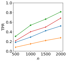
(a)

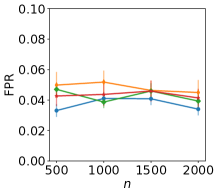
(b)

Figure 3: Logistic experiment as $n$ increases. Results are shown for $\mathrm{\widehat{HSIC}}_{Blo}$ and $\mathrm{\widehat{HSIC}}_{Inc}$.

5.2 Benchmarks

We apply MultiMMD and PolyMMD for selecting features that significantly distinguishes two samples. Since TPR and FPR requires the knowledge of true features which is unknown, we regard the original $d^{\prime}$ number of pre-processed features in the dataset as “true” features and then we augment the dataset with $30$ fake features. This problem was studied by Yamada et al., (2019). We apply our proposal to three datasets.

Pulsar dataset ($n=100,\ d^{\prime}=8$) of Lyon et al., (2016) contain samples of pulsar candidates collected during the High Time Resolution Universe Survey. We split the dataset into two sets where one is for pulsars and the other for not pulsars.

Heart dataset $(n=138,\ d^{\prime}=13)$ of Janosi et al., (1988) contains samples of patients, their attributes (such as age and sex) and whether they suffer from heart disease. We split the dataset by whether they have heart disease or not.

Wine dataset $(n=100,\ d^{\prime}=12)$ of Cortez et al., (2009) contains samples related to red and white variants of the Portuguese “Vinho Verde” wine. The dataset is split into red and white wines.

	PolyMMD		MultiMMD
Dataset	TPR	FPR	TPR	FPR
Pulsar	0.746	0.063	0.993	0.056
Heart	0.359	0.042	0.588	0.049
Wine	0.567	0.054	0.749	0.057

Table 1: Benchmarking experiment using $\mathrm{MMD}_{Inc}$. The results are averaged over $100$ trials ($\alpha=0.05$).

The results are shown in Table 1. It can be seen that TPR of our proposed method is higher than PolySel for all datasets while both methods corroborate with the theory that the FPR is controlled at $\alpha$ in all scenarios.

5.3 Anomalous Dataset Detection

In this experiment, we are given $6$ datasets with one desired reference set and our goal is to eliminate the datasets that deviate too far from the reference. To be specific, our datasets are formed from the smiling subset of the CelebA dataset (Liu et al.,, 2015), it may also contain synthetic samples generated from the smiling GAN of Jitkrittum et al., (2018). Instead of testing on raw pixels, the datasets are pre-processed and represented by $2048$-dimensional features extracted from the Pool3 layer of Inception-v3 (Szegedy et al.,, 2016). Each dataset contains $1000$ samples with $x\%$ being fake images and $1-x\%$ real images. In this case, since all models are wrong (Box,, 1976), the higher percentage of the presence of synthetic samples, the higher the chance of rejection. We apply MultiSel and PolySel with the IMQ kernel (Gorham and Mackey,, 2017).

Dataset	1	2	3	4	5	6
$\%$ Fakes	$0\%$	$10\%$	$20\%$	$30\%$	$40\%$	$50\%$
MultiMMD	0.03	0.02	0.07	0.06	0.27	0.49
PolyMMD	0.02	0.02	0.05	0.04	0.28	0.45

Table 2: Rejection rate of five datasets for both MultiSel and PolySel. Each dataset has its own percentage of fake features. These results were averaged over $100$ trials and we set $k=4$, $\alpha=0.05$ and $n=2000$.

The results are shown in Table 2. The rejection rates of both methods are similar. Dataset 1 has the same distribution as our reference model and so the rejection rate of less than $\alpha$. As for the other datasets, the rejection rate increases as the percentage of fake increases but the similarity in the performance is expected and can be explained by the small difference in the selection event for PolyMMD and MultiMMD.

Acknowledgements

M.Y. was supported by the JST PRESTO program JPMJPR165A and partly supported by MEXT KAKENHI 16H06299 and the RIKEN engineering network funding. S.M. was supported by MEXT KAKENHI 16H06299.

More Powerful Selective Kernel Tests for Feature Selection

Supplementary

Appendix A TRUE POSITIVE RATE (TPR) AND FALSE POSITIVE RATE (FPR)

Let $\mathcal{I}_{-}$ be the indices of features such that the null holds, i.e., for MMD, we have $\mathcal{I}_{-}:=\{i:\mathrm{MMD}(P^{(i)},Q^{(i)})=0\}$ (and for HSIC, we have $\mathcal{I}_{-}:=\{i:\mathrm{HSIC}(P^{(i)},Q)=0\}$). Similarly, let $\mathcal{I}_{+}$ be the indices of features such that the alternative holds, i.e., for MMD, we have $\mathcal{I}_{+}:=\{i:\mathrm{MMD}(P^{(i)},Q^{(i)})>0\}$ (and for HSIC, we have $\mathcal{I}_{+}:=\{i:\mathrm{HSIC}(P^{(i)},Q)>0\}$). Then, for a set of selected features $\mathcal{S}_{k}$ we define FPR and TPR as follows,

$$\mathrm{FPR}=\mathbb{E}\bigg{[}\frac{|\mathcal{S}_{k}\cap\mathcal{I}_{-}\cap\mathcal{R}|}{|\mathcal{S}_{k}\cap\mathcal{I}_{-}|}\bigg{]}, \mathrm{TPR}=\mathbb{E}\bigg{[}\frac{|\mathcal{S}_{k}\cap\mathcal{I}_{+}\cap\mathcal{R}|}{|\mathcal{S}_{k}\cap\mathcal{I}_{+}|}\bigg{]},$$

where $\mathcal{R}$ is the set of indices that the algorithm rejections and note that $\mathcal{R}\subseteq\mathcal{S}_{k}$.

Appendix B EMPIRICAL DISTRIBUTIONS OF $\widehat{\mathrm{MMD}}_{\text{Inc}}(X,Y)$ and $\widehat{\mathrm{HSIC}}_{\text{Inc}}(Z)$

In this section, we simulate the empirical distribution of the incomplete estimator for both $\widehat{\mathrm{MMD}}_{\text{Inc}}(X,Y)$ and $\widehat{\mathrm{HSIC}}_{\text{Inc}}(Z)$.

B.1 Empirical distribution of $\widehat{\mathrm{MMD}}_{\text{Inc}}(X,Y)$

Case $P=Q$: For MMD, we let $X\sim\mathcal{N}(0,1)$ and $Y\sim\mathcal{N}(0,1)$ which means $\widehat{\mathrm{MMD}}_{\text{u}}(X,Y)$ is degenerate whereas we show that $\widehat{\mathrm{MMD}}_{\text{Inc}}(X,Y)$ follows a normal distribution (see Figure 4). When the $r$ is small, the empirical distribution of the incomplete estimators follows a normal distribution butas $r$ gets bigger we expect it to behave like its complete estimator counterpart.

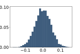
(a) $r=1$

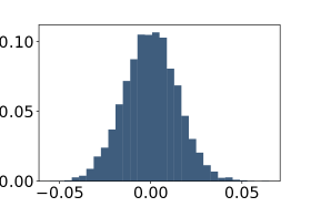
(b) $r=10$

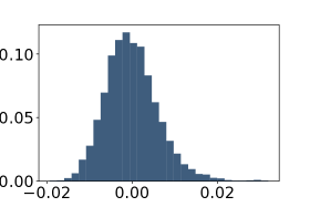
(c) $r=100$

Figure 4: The empirical distribution $\widehat{\mathrm{MMD}}_{\text{Inc}}(X,Y)$ for $r\in\{1,10,100\}$. $5000$ samples were used.

Case $P\neq Q$: We show the empirical distribution of the incomplete estimator for MMD when $P=\mathcal{N}(0,1)$ and $Q=\mathcal{N}(\mu,1)$ and $\mu\in\{0,2,3\}$. Under the alternative, for our choice in $r$, the distribution under the alternative is expected to have higher variance than the null distribution.

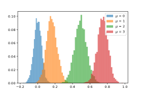
(a) $r=1$

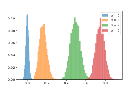
(b) $r=10$

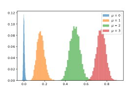
(c) $r=100$

Figure 5: The empirical distribution $\widehat{\mathrm{MMD}}_{\text{Inc}}(Z)$ for $r\in\{1,10,100\}$. $5000$ samples were used.

B.2 Empirical distribution of $\widehat{\mathrm{HSIC}}_{\text{Inc}}(Z)$

For HSIC, let $Z:=(X,Y)$ where $X$ and $Y$ is follows a standard normal and is sampled independently of each other. We show that in this case $\widehat{\mathrm{HSIC}}_{\text{Inc}}(Z)$ is also normal (see Figure 6).

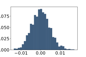
(a) $r=1$

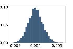
(b) $r=10$

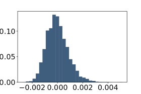
(c) $r=100$

Figure 6: The empirical distribution $\widehat{\mathrm{HSIC}}_{\text{Inc}}(X,Y)$ for $r\in\{1,10,100\}$. $5000$ samples were used.

Appendix C MULTISCALE BOOSTRAP ALGORITHM FOR HSIC

In this section, we present algorithms for MultiHSIC for incomplete HSIC (Section C.1) and for block HSIC (Section C.2). Algorithm 3 describes the procedure for calculating $p$-values using multiscale bootstrap.

C.1 Incomplete HSIC

The parameters $\bm{T}(\bm{Z})$ and $\bm{\Sigma}$ for the incomplete estimator are estimated with the same method as for the incomplete MMD (see Section 3). The algorithm is described in Algorithm 3.

Algorithm 3 MultiHSIC($\bm{Z}_{n},k,\,\mathcal{M}$): Selective $p$-values for the null hypothesis $H_{0,i}:\mathrm{HSIC}(P_{\bm{x}^{(i)}\bm{y}})=0\ |\ i\in\mathcal{S}_{k}\text{ is selected}$.

1:$\hat{\bm{T}}(\bm{Z}),\hat{\bm{\Sigma}}\leftarrow$EstimateParam($\bm{Z}_{n}$)

2:$\mathcal{S}_{k}\leftarrow$ the indexes of $k$ largest values of $\{\widehat{\mathrm{HSIC}}(\bm{Z}_{n}^{(i)})\}_{i\in\mathcal{I}}$

3:for $i\in\mathcal{S}_{k}$ do

4:     for $n^{\prime}\in\mathcal{M}$ do

5:         $\gamma^{2}_{n^{\prime}}\leftarrow\frac{n}{n^{\prime}}$

6:         Sample $\{\bm{y}^{*}_{i}\}^{B}_{i=1}\overset{i.i.d.}{\sim}\mathcal{N}(\hat{\bm{T}}(\bm{Z}),\,\gamma^{2}_{n^{\prime}}\hat{\bm{\Sigma}})$

7:         $\textrm{BP}_{\gamma_{n^{\prime}}^{2}}(S)\leftarrow\sum^{B}_{i=1}\mathds{1}^{(i)}_{S}(\bm{y}^{*}_{i})/B$

8:     end for

9:     Fit a linear model $\varphi_{S}(\gamma^{2})$ such that $\varphi_{S}(\gamma^{2})=\gamma\bar{\Phi}^{-1}(\textrm{BP}_{\gamma^{2}}(S))$.

10:     $\hat{\beta}_{0}^{(i)}\leftarrow\hat{\sigma}_{i}^{-1}\sqrt{l_{n}}\widehat{\mathrm{HSIC}}_{Inc}(\bm{Z}_{n}^{(i)})$

11:     $p_{i}\leftarrow\bar{\Phi}(\hat{\beta}_{0}^{(i)})/\bar{\Phi}(\hat{\beta}_{0}^{(i)}+\varphi_{S}(0))$

12:end for

13:return $\{p_{i}\}_{i=0}^{k}$ and $\mathcal{S}_{k}$

The following theorem justifies our use of the multivariate normal model,

Theorem 1.

Assume that $\lim_{n,l\rightarrow\infty}n^{-1}l=\lambda$ and assume that $\lim_{n,l\rightarrow\infty}n^{-2}l=0$ and $0<\lambda<\infty$ then, $l^{\frac{1}{2}}\bigg{(}\begin{bmatrix}\widehat{\mathrm{HSIC}}_{Inc}(\bm{Z}^{(1)})\\ \vdots\\ \widehat{\mathrm{HSIC}}_{Inc}(\bm{Z}^{(d)})\end{bmatrix}-\begin{bmatrix}\mathrm{HSIC}(P_{\bm{x}^{(1)}\bm{y}})\\ \vdots\\ \mathrm{HSIC}(P_{\bm{x}^{(d)}\bm{y}})\end{bmatrix}\bigg{)}$ is asymptotically normal.

The proof can be found in Appendix D.

C.2 Block HSIC

Block estimator as the incomplete estimator: The block estimator $\mathrm{\widehat{HSIC}}_{Blo}$ (Zhang et al.,, 2018) is an example of an incomplete estimator for HSIC with a fixed design matrix. To see this note that for a given blocksize $B$, we have a total of $\frac{n}{B}$ blocks. For each block, the complete U-statistic estimator is calculated, i.e., for block $t$

$$\hat{\eta}(t)=\frac{(B-4)!}{B!}\sum_{(i,j,q,r)\in\mathbf{i}^{[(t-1)B+1,tB]}_{4}}h(i,j,q,r),$$

where $\mathbf{i}^{[u,i]}_{4}$ is the set of 4-tuple with each index, between $u$ and $i$, appearing exactly once. There are a total of $\frac{n}{B}$ blocks that are averaged to produce $\mathrm{\widehat{HSIC}}_{Blo}$, i.e., we have

$$\mathrm{\widehat{HSIC}}_{Blo}=\frac{B}{n}\sum_{t=1}^{\frac{n}{B}}\hat{\eta}(t).$$

Thus, we have shown that $\mathrm{\widehat{HSIC}}_{Blo}$ can be rewritten as $\widehat{\mathrm{HSIC}}_{Inc}$ where we have $\mathcal{D}=\cup_{t=1}^{\frac{n}{B}}\mathbf{i}^{[(t-1)B+1,tB]}_{4}$. Note that $|\mathcal{D}_{Blo}|=\frac{(B-1)!}{(B-4)!}n$.

Algorithm: The extension to multiscale bootstrap to include the block estimator is simple. It only requires changes in the parameters of the resampling distribution for varying $n^{\prime}$, as a well as how the signed distance $\hat{\beta}^{(i)}_{0}$ for feature $i$ is calculated.

Let $\hat{\bm{T}}(\bm{Z}):=\sqrt{\frac{n}{B}}[\widehat{\mathrm{HSIC}}_{Blo}(\bm{Z}_{n}^{(1)}),\dots,\widehat{\mathrm{HSIC}}_{Blo}(\bm{Z}_{n}^{(d)})]^{\top}$ and $\bm{T}(\bm{Z})$ be its population counterpart, namely, $\bm{T}(\bm{Z})=\sqrt{\frac{n}{B}}[{\mathrm{HSIC}}(P_{\bm{x}^{(1)}\bm{y}}),\dots,{\mathrm{HSIC}}(P_{\bm{x}^{(d)}\bm{y}})]^{\top}$. Note that $\hat{\bm{T}}(\bm{Z})$ can be equivalently written as $\sum_{i=1}^{n/B}\hat{\bm{\eta}}(i)$ where $\hat{\bm{\eta}}(i)=[\hat{\eta}^{(1)}(i),\dots,\hat{\eta}^{(d)}(i)]^{\top}$, and $\hat{\eta}^{(j)}(i)$ is the complete U-statistic estimator for HSIC applied to the $i$-th block of $\bm{Z}^{(j)}$. Then in the limit $n\rightarrow\infty$, $B\rightarrow\infty$, and $\frac{n}{B}\rightarrow\infty$ (Zhang et al.,, 2018), we have under the null hypothesis

$$\hat{\bm{T}}(\bm{Z})-\bm{T}(\bm{Z})\sim\mathcal{N}(\bm{0},\,\bm{\Sigma}),$$

where $\bm{\Sigma}$ is the covariance matrix with its elements as $\bm{\Sigma}_{ij}=\mathrm{Cov}\left(\bm{\eta}^{\left(i\right)},\bm{\eta}^{\left(j\right)}\right)$. We estimate $\bm{\Sigma}$ with the sample covariance $\hat{\bm{\Sigma}}$, i.e., we have $\hat{\bm{\Sigma}}:=\frac{B}{n}\sum_{i=1}^{n/B}[\hat{\bm{\eta}}(i)-\overline{\bm{\eta}}][\hat{\bm{\eta}}(i)-\overline{\bm{\eta}}]^{\top}$. Then for varying $n^{\prime}$, instead of resampling $n^{\prime}$ samples from $\bm{Z}$, we produce samples directly from $\mathcal{N}(\hat{\bm{T}}(\bm{Z}),\frac{n}{n^{\prime}}\hat{\bm{\Sigma}})$ as before. The sign distance $\hat{\beta}_{0}^{(i)}$ is $\hat{\sigma}_{i}^{-1}\sqrt{\frac{n}{B}}\widehat{\mathrm{HSIC}}_{Blo}(\bm{Z}_{n}^{(i)})$ where $\hat{\sigma}_{i}^{-1}$ is the $i$-th diagonal element of $\hat{\bm{\Sigma}}$.

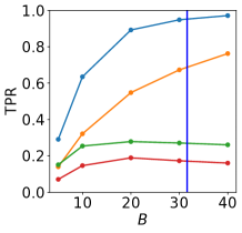
(a)

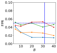
(b)

Figure 7: Logistic experiment. $B$ increases for $\mathrm{\widehat{HSIC}}_{B}$. We use a Gaussian kernel with its bandwidth either set to be $1$ or chosen with the median heuristic. We use $n=1000$.

Empirical Results: In this experiment, we use the same setup as Figure 3 for the Logit problem and the results are shown in Figure 7. Our aim is to investigate the behaviour of our test when $B$ the block size increases. In Zaremba et al., (2013, Section 5), they investigated the behaviour of the block estimator under finite samples and found that there can have severe bias under the null hypothesis.

In our results, we observed that there was a large deviation for the nominal size $\alpha$ and an increase in the TPR. We speculate that this is due to the positive bias in finite samples of the skewness of the block estimator. These experiments show that the effect is more pronounced for MultiHSIC (than PolyHSIC) which may be because of our choice in parameterising the bootstrap samples as a normal distribution. We note that the effect of FPR going below the nominal $\alpha$ is not just for very large values of $B$ but even for the recommended heuristic $B=\sqrt{n}$. It would be interesting to investigate this problem and correct for it in future works.

Appendix D PROOFS

In this section, we provide proofs for our statements in Section 4. Before we begin, recall that

$$h(i,j,q,r)=\frac{1}{4!}\sum_{(s,t,u,v)}^{(i,j,q,r)}\bm{K}_{st}[\bm{L}_{st}+\bm{L}_{uv}-2\bm{L}_{su}]$$

is the order-$4$ U-statistic kernel for HSIC. We define the conditional expectation of the U-statistic kernel

$$h_{4} =h(i,j,q,r),$$

$$h_{3} =\mathbb{E}[h(i,j,q,r)\,|\,i,\,j,\,q\,],$$

$$h_{2} =\mathbb{E}[h(i,j,q,r)\,|\,i,\,j\,]$$

$$h_{1} =\mathbb{E}[h(i,j,q,r)\,|\,i\,].$$

Let $c$ be the smallest integer such that $h_{c}\neq\mathrm{HSIC}$. When $P\mathchoice{\mathrel{\hbox to0.0pt{$\displaystyle\perp$\hss}\mkern 2.0mu{\displaystyle\perp}}}{\mathrel{\hbox to0.0pt{$\textstyle\perp$\hss}\mkern 2.0mu{\textstyle\perp}}}{\mathrel{\hbox to0.0pt{$\scriptstyle\perp$\hss}\mkern 2.0mu{\scriptstyle\perp}}}{\mathrel{\hbox to0.0pt{$\scriptscriptstyle\perp$\hss}\mkern 2.0mu{\scriptscriptstyle\perp}}}Q$, we have $h_{1}=0$ and $\mathrm{HSIC}=h_{1}$ so $c>1$. However when $P\not\!\perp\!\!\!\perp Q$, $h_{1}\neq\mathrm{HSIC}$ so $c=1$. Similarly, we show that $\widehat{\mathrm{HSIC}}_{Inc}$ is asymptotically normal under mild assumptions.

Theorem 2 (Asymptotic Distribution of $\widehat{\mathrm{HSIC}}_{Inc}$).

Let $c$ be the smallest integer such that $h_{c}\neq\mathrm{HSIC}$ ($h_{c}$ defined in Appendix D) and let $\lim_{n,l\rightarrow\infty}n^{-c}l=\lambda$ $(0\leq\lambda\leq\infty)$ and let $\mathcal{D}$ be constructed by selecting $l$ subsets with replacement from $\bm{i}^{n}_{4}$ then,

1. If $\lambda=0$ then, $l^{\frac{1}{2}}(\widehat{\mathrm{HSIC}}_{\text{Inc}}(\bm{z})-\mathrm{HSIC}(P_{xy})\overset{d}{\rightarrow}\mathcal{N}(0,\sigma^{2})$,

2. If $0<\lambda<\infty$ then, $l^{\frac{1}{2}}(\widehat{\mathrm{HSIC}}_{\text{Inc}}(\bm{z})-\mathrm{HSIC}(P_{xy}))\overset{d}{\rightarrow}\lambda^{\frac{1}{2}}V+T$,

3. If $\lambda=\infty$ then, $n^{\frac{c}{2}}(\widehat{\mathrm{HSIC}}_{\text{Inc}}(\bm{z})-\mathrm{HSIC}(P_{xy}))\overset{d}{\rightarrow}V$,

where $V$ is a random variable with the limit distribution of $n^{c/2}(\widehat{\mathrm{HSIC}}_{\text{u}}(\bm{z})-\mathrm{HSIC})$ and $T\sim\mathcal{N}(0,\sigma^{2})$ where $\sigma^{2}=\mathrm{Var}[h(i,j,q,r)]$.

Proof.

See Janson, (1984, Corollary 1) and Lee, (2019, Theorem 1, Section 4.3.3) ∎

See 1

Proof.

When $P\mathchoice{\mathrel{\hbox to0.0pt{$\displaystyle\perp$\hss}\mkern 2.0mu{\displaystyle\perp}}}{\mathrel{\hbox to0.0pt{$\textstyle\perp$\hss}\mkern 2.0mu{\textstyle\perp}}}{\mathrel{\hbox to0.0pt{$\scriptstyle\perp$\hss}\mkern 2.0mu{\scriptstyle\perp}}}{\mathrel{\hbox to0.0pt{$\scriptscriptstyle\perp$\hss}\mkern 2.0mu{\scriptscriptstyle\perp}}}Q$, then $c\geq 2$ then the result immediately follows from Theorem 2 for the case $\lambda=0$.

For $P\not\!\perp\!\!\!\perp Q$, then $c=1$ thus, under our assumptions, we obtain our result from Theorem 2. ∎

See 1

Proof.

This proof is identical to the proof of Yamada et al., (2019, Theorem 5). From Cramér-Wold theorem, it is sufficient to prove that for every $\bm{\eta}\in\mathbb{R}^{d}$,

$$\bm{\eta}^{\top}\begin{bmatrix}\widehat{\mathrm{HSIC}}_{Inc}(\bm{Z}^{(1)})\\ \vdots\\ \widehat{\mathrm{HSIC}}_{Inc}(\bm{Z}^{(d)})\end{bmatrix}\overset{d}{\rightarrow}\bm{\eta}^{\top}\bm{V}$$

where $\bm{V}$ is some normal distribution. Under our assumptions, for all $i$ $\widehat{\mathrm{HSIC}}_{Inc}(\bm{Z}^{(i)})$ follows a normal distribution. Following from the continuous mapping theorem, for all $\bm{\eta}\in\mathbb{R}^{d}$ we have as desired. ∎

Appendix E Additional Experiments

In this section, we provide additional experiments with HSIC. The first is a benchmarking experiment similar to the one performed in Section 5.2. The second uses the Divorce dataset (Yöntem et al.,, 2019) where people were given a questionnaire about their marriage and asked to rate each statement about their marriage from 0 to 4 depending on the truthfulness.

E.1 Benchmark

The goal is to rediscover the original features with statistical significance. As seen in the Table 3, the results indicate that MultiSel achieves higher power (as with the MMD).

	MultiSel-HSIC		PolySel-HSIC
Dataset	TPR	FPR	TPR	FPR
Pulsar ($n=100$)	$0.705$	$0.023$	$0.625$	$0.025$
Heart ($n=138$)	$0.469$	$0.029$	$0.410$	$0.030$
Wine ($n=200$)	$0.800$	$0.042$	$0.730$	$0.058$

Table 3: The TPR and FPR for the benchmarking experiment using $\widehat{\mathrm{HSIC}}_{Inc}$. The results are averaged over $100$ trials, with $\alpha=0.05$.

E.2 Divorce Dataset

We report the calculated $p$-values of each statistical test of dependency between a selected statement and the outcome of divorce. In the experiment, we chose $r=15$, $k=15$ (out of $54$) and $n=150$ with the results summaries in Table 4. We found that MultiSel declared $6$ more statements as significantly (than PolySel) with a significance level at $\alpha=0.05$, including statements such as “I feel aggressive when I argue with my wife.” and “My wife and most of our goals are common.”. We do not know the ground truth but the $6$ statements seem plausible. The results suggest that MultiSel has higher detection rate.

	$p$-values
	MultiSel-HSIC	PolySel-HSIC
My argument with my wife is not calm.	<0.01	<0.01
Fights often occur suddenly.	<0.01	0.41
I can insult my spouse during our discussions.	<0.01	0.09
When fighting with my spouse, I usually use expressions such as ‘you always’ or ‘you never’.	<0.01	0.17
We’re compatible with my wife about what love should be.	<0.01	0.43
My wife and most of our goals are common.	<0.01	0.25
I feel aggressive when I argue with my wife.	<0.01	0.22
We’re starting a fight before I know what’s going on.	<0.01	<0.01
I can use negative statements about my wife’s personality during our discussions.	<0.01	0.05
I hate my wife’s way of bringing it up.	<0.01	<0.01
I enjoy our holidays with my wife.	0.12	0.27
When we fight, I remind her of my wife’s inadequate issues.	0.13	0.04
When I argue with my wife, it will eventually work for me to contact him.	0.16	0.14
I know my wife’s hopes and wishes.	0.77	0.56
I can use offensive expressions during our discussions.	0.94	0.89

Table 4: The resultant $p$-values from one trial of the divorce dataset using $\mathrm{HSIC}_{Inc}$.

References

- Barber et al., (2019) Barber, R. F., Candès, E. J., et al. (2019). A knockoff filter for high-dimensional selective inference. The Annals of Statistics, 47(5):2504–2537.
- Benjamini and Hochberg, (1995) Benjamini, Y. and Hochberg, Y. (1995). Controlling the false discovery rate: a practical and powerful approach to multiple testing. Journal of the Royal statistical society: series B (Methodological), 57(1):289–300.
- Blom, (1976) Blom, G. (1976). Some properties of incomplete u-statistics. Biometrika, 63(3):573–580.
- Box, (1976) Box, G. E. (1976). Science and statistics. Journal of the American Statistical Association, 71(356):791–799.
- Candes et al., (2018) Candes, E., Fan, Y., Janson, L., and Lv, J. (2018). Panning for gold: ’model-X’ knockoffs for high dimensional controlled variable selection. Journal of the Royal Statistical Society: Series B (Statistical Methodology), 80(3):551–577.
- Candès et al., (2016) Candès, E. J., Fan, Y., Janson, L., and Lv, J. (2016). Panning for gold: Model-free knockoffs for high-dimensional controlled variable selection. Department of Statistics, Stanford University.
- Cortez et al., (2009) Cortez, P., Cerdeira, A., Almeida, F., Matos, T., and Reis, J. (2009). Modeling wine preferences by data mining from physicochemical properties. Decision Support Systems, 47(4):547–553.
- Efron et al., (1996) Efron, B., Halloran, E., and Holmes, S. (1996). Bootstrap confidence levels for phylogenetic trees. Proceedings of the National Academy of Sciences, 93(23):13429–13429.
- Efron et al., (1998) Efron, B., Tibshirani, R., et al. (1998). The problem of regions. The Annals of Statistics, 26(5):1687–1718.
- Fithian et al., (2014) Fithian, W., Sun, D., and Taylor, J. (2014). Optimal inference after model selection. arXiv preprint arXiv:1410.2597.
- Fithian et al., (2015) Fithian, W., Taylor, J., Tibshirani, R., and Tibshirani, R. (2015). Selective sequential model selection. arXiv preprint arXiv:1512.02565.
- Fukumizu et al., (2008) Fukumizu, K., Gretton, A., Sun, X., and Schölkopf, B. (2008). Kernel measures of conditional dependence. In Advances in neural information processing systems, pages 489–496.
- Gelman and Loken, (2013) Gelman, A. and Loken, E. (2013). The garden of forking paths: Why multiple comparisons can be a problem, even when there is no “fishing expedition” or “p-hacking” and the research hypothesis was posited ahead of time. Department of Statistics, Columbia University.
- Gorham and Mackey, (2017) Gorham, J. and Mackey, L. (2017). Measuring sample quality with kernels. In Proceedings of the 34th International Conference on Machine Learning-Volume 70, pages 1292–1301. JMLR. org.
- Gretton et al., (2012) Gretton, A., Borgwardt, K. M., Rasch, M. J., Schölkopf, B., and Smola, A. (2012). A kernel two-sample test. Journal of Machine Learning Research, 13(Mar):723–773.
- Gretton et al., (2005) Gretton, A., Bousquet, O., Smola, A., and Schölkopf, B. (2005). Measuring statistical dependence with Hilbert-Schmidt norms. In International conference on algorithmic learning theory, pages 63–77. Springer.
- Gretton et al., (2008) Gretton, A., Fukumizu, K., Teo, C. H., Song, L., Schölkopf, B., and Smola, A. J. (2008). A kernel statistical test of independence. In Advances in neural information processing systems, pages 585–592.
- Hoeffding, (1992) Hoeffding, W. (1992). A class of statistics with asymptotically normal distribution. In Breakthroughs in Statistics, pages 308–334. Springer.
- Janosi et al., (1988) Janosi, A., Steinbrunn, W., Pfisterer, M., and Detrano, R. (1988). Uci machine learning repository-heart disease dataset.
- Janson, (1984) Janson, S. (1984). The asymptotic distributions of incomplete U-statistics. Zeitschrift für Wahrscheinlichkeitstheorie und Verwandte Gebiete, 66(4):495–505.
- Jitkrittum et al., (2018) Jitkrittum, W., Kanagawa, H., Sangkloy, P., Hays, J., Schölkopf, B., and Gretton, A. (2018). Informative features for model comparison. In Advances in Neural Information Processing Systems, pages 808–819.
- Jordon et al., (2018) Jordon, J., Yoon, J., and van der Schaar, M. (2018). KnockoffGAN: Generating knockoffs for feature selection using generative adversarial networks.
- Lee, (2019) Lee, A. J. (2019). U-statistics: Theory and Practice. Routledge.
- Lee et al., (2016) Lee, J. D., Sun, D. L., Sun, Y., Taylor, J. E., et al. (2016). Exact post-selection inference, with application to the lasso. The Annals of Statistics, 44(3):907–927.
- Lim et al., (2019) Lim, J. N., Yamada, M., Schölkopf, B., and Jitkrittum, W. (2019). Kernel stein tests for multiple model comparison. In Advances in Neural Information Processing Systems, pages 2240–2250.
- Liu et al., (2018) Liu, K., Markovic, J., and Tibshirani, R. (2018). More powerful post-selection inference, with application to the Lasso. arXiv preprint arXiv:1801.09037.
- Liu et al., (2015) Liu, Z., Luo, P., Wang, X., and Tang, X. (2015). Deep learning face attributes in the wild. In Proceedings of International Conference on Computer Vision (ICCV).
- Lu et al., (2018) Lu, Y., Fan, Y., Lv, J., and Noble, W. S. (2018). DeepPINK: reproducible feature selection in deep neural networks. In Advances in Neural Information Processing Systems, pages 8676–8686.
- Lyon et al., (2016) Lyon, R. J., Stappers, B., Cooper, S., Brooke, J., and Knowles, J. (2016). Fifty years of pulsar candidate selection: from simple filters to a new principled real-time classification approach. Monthly Notices of the Royal Astronomical Society, 459(1):1104–1123.
- Romano et al., (2019) Romano, Y., Sesia, M., and Candès, E. (2019). Deep knockoffs. Journal of the American Statistical Association, (just-accepted):1–27.
- Serfling, (2009) Serfling, R. J. (2009). Approximation theorems of mathematical statistics, volume 162. John Wiley & Sons.
- Shimodaira, (2002) Shimodaira, H. (2002). An approximately unbiased test of phylogenetic tree selection. Systematic biology, 51(3):492–508.
- Shimodaira, (2008) Shimodaira, H. (2008). Testing regions with nonsmooth boundaries via multiscale bootstrap. Journal of Statistical Planning and Inference, 138(5):1227–1241.
- Shimodaira, (2014) Shimodaira, H. (2014). Higher-order accuracy of multiscale-double bootstrap for testing regions. Journal of Multivariate Analysis, 130:208–223.
- Shimodaira et al., (2004) Shimodaira, H. et al. (2004). Approximately unbiased tests of regions using multistep-multiscale bootstrap resampling. The Annals of Statistics, 32(6):2616–2641.
- Shimodaira and Terada, (2019) Shimodaira, H. and Terada, Y. (2019). Selective inference for testing trees and edges in phylogenetics. Frontiers in Ecology and Evolution, 7:174.
- Simmons et al., (2011) Simmons, J. P., Nelson, L. D., and Simonsohn, U. (2011). False-positive psychology: Undisclosed flexibility in data collection and analysis allows presenting anything as significant. Psychological science, 22(11):1359–1366.
- Slim et al., (2019) Slim, L., Chatelain, C., Azencott, C.-A., and Vert, J.-P. (2019). kernelpsi: a post-selection inference framework for nonlinear variable selection. In International Conference on Machine Learning, pages 5857–5865.
- Smola et al., (2007) Smola, A., Gretton, A., Song, L., and Schölkopf, B. (2007). A Hilbert space embedding for distributions. In International Conference on Algorithmic Learning Theory, pages 13–31. Springer.
- Song et al., (2012) Song, L., Smola, A., Gretton, A., Bedo, J., and Borgwardt, K. (2012). Feature selection via dependence maximization. Journal of Machine Learning Research, 13(May):1393–1434.
- Szegedy et al., (2016) Szegedy, C., Vanhoucke, V., Ioffe, S., Shlens, J., and Wojna, Z. (2016). Rethinking the inception architecture for computer vision. In Proceedings of the IEEE conference on computer vision and pattern recognition, pages 2818–2826.
- Terada and Shimodaira, (2017) Terada, Y. and Shimodaira, H. (2017). Selective inference for the problem of regions via multiscale bootstrap. arXiv preprint arXiv:1711.00949.
- Terada and Shimodaira, (2019) Terada, Y. and Shimodaira, H. (2019). Selective inference after variable selection via multiscale bootstrap. arXiv preprint arXiv:1905.10573.
- Tian et al., (2018) Tian, X., Taylor, J., et al. (2018). Selective inference with a randomized response. The Annals of Statistics, 46(2):679–710.
- Tibshirani et al., (2016) Tibshirani, R. J., Taylor, J., Lockhart, R., and Tibshirani, R. (2016). Exact post-selection inference for sequential regression procedures. Journal of the American Statistical Association, 111(514):600–620.
- Yamada et al., (2018) Yamada, M., Umezu, Y., Fukumizu, K., and Takeuchi, I. (2018). Post selection inference with kernels. In Proceedings of the Twenty-First International Conference on Artificial Intelligence and Statistics, volume 84 of Proceedings of Machine Learning Research, pages 152–160, Playa Blanca, Lanzarote, Canary Islands. PMLR.
- Yamada et al., (2019) Yamada, M., Wu, D., Tsai, Y.-H. H., Ohta, H., Salakhutdinov, R., Takeuchi, I., and Fukumizu, K. (2019). Post selection inference with incomplete maximum mean discrepancy estimator. In International Conference on Learning Representations.
- Yöntem et al., (2019) Yöntem, M. K., Adem, K., İlhan, T., and Kılıçarslan, S. (2019). Divorce prediction using correlation based feature selection and artificial neural networks. Nevşehir Hacı Bektaş Veli Üniversitesi SBE Dergisi, 9(1):259–273.
- Zaremba et al., (2013) Zaremba, W., Gretton, A., and Blaschko, M. (2013). B-test: A non-parametric, low variance kernel two-sample test. In Advances in neural information processing systems, pages 755–763.
- Zhang et al., (2018) Zhang, Q., Filippi, S., Gretton, A., and Sejdinovic, D. (2018). Large-scale kernel methods for independence testing. Statistics and Computing, 28(1):113–130.