Curve Based Approximation of Measures on Manifolds by Discrepancy Minimization

Abstract

The approximation of probability measures on compact metric spaces and in particular on Riemannian manifolds by atomic or empirical ones is a classical task in approximation and complexity theory with a wide range of applications. Instead of point measures we are concerned with the approximation by measures supported on Lipschitz curves. Special attention is paid to push-forward measures of Lebesgue measures on the unit interval by such curves. Using the discrepancy as distance between measures, we prove optimal approximation rates in terms of the curve’s length and Lipschitz constant. Having established the theoretical convergence rates, we are interested in the numerical minimization of the discrepancy between a given probability measure and the set of push-forward measures of Lebesgue measures on the unit interval by Lipschitz curves. We present numerical examples for measures on the 2- and 3-dimensional torus, the 2-sphere, the rotation group on $\mathbb{R}^{3}$ and the Grassmannian of all 2-dimensional linear subspaces of $\mathbb{R}^{4}$. Our algorithm of choice is a conjugate gradient method on these manifolds which incorporates second-order information. For efficiently computing the gradients and the Hessians within the algorithm, we approximate the given measures by truncated Fourier series and use fast Fourier transform techniques on these manifolds.

The approximation of probability measures by atomic or empirical ones based on their discrepancies is a well examined problem in approximation and complexity theory [59, 62, 67] with a wide range of applications, e.g., in the derivation of quadrature rules and in the construction of designs. Recently, discrepancies were also used in image processing for dithering [46, 72, 77], i.e., for representing a gray-value image by a finite number of black dots, and in generative adversarial networks [29].

Besides discrepancies, Optimal Transport (OT) and in particular Wasserstein distances have emerged as powerful tools to compare probability measures in recent years, see [24, 81] and the references therein. In fact, so-called Sinkhorn divergences, which are computationally much easier to handle than OT, are known to interpolate between OT and discrepancies [31]. For the sample complexity of Sinkhorn divergences we refer to [38]. The rates for approximating probability measures by atomic or empirical ones with respect to Wasserstein distances depend on the dimension of the underlying spaces, see [21, 58]. In contrast, approximation rates based on discrepancies can be given independently of the dimension [67], i.e., they do not suffer from the curse of dimensionality. Additionally, we should keep in mind that the computation of discrepancies does not involve a minimization problem, which is a major drawback of OT and Sinkhorn divergences. Moreover, discrepancies admit a simple description in Fourier domain and hence the use of fast Fourier transforms is possible, leading to better scalability than the aforementioned methods.

Instead of point measures, we are interested in approximations with respect to measures supported on curves. More precisely, we consider push-forward measures of probability measures $\omega\in{\mathcal{P}}([0,1])$ by Lipschitz curves of bounded speed, with special focus on absolutely continuous measures $\omega=\rho\lambda$ and the Lebesgue measure $\omega=\lambda$. In this chapter, we focus on approximation with respect to discrepancies. For related results on quadrature and approximation on manifolds, we refer to [32, 47, 64, 65] and the references therein. An approximation model based on the 2-Wasserstein distance was proposed in [61]. That work exploits completely different techniques than ours both in the theoretical and numerical part. Finally, we want to point out a relation to principal curves which are used in computer science and graphics for approximating distributions approximately supported on curves [49, 50, 55, 50, 57]. For the interested reader, we further comment on this direction of research in Remark 2.4 and in the conclusions. Next, we want to motivate our framework by numerous potential applications:

• In MRI sampling [11, 17], it is desirable to construct sampling curves with short sampling times (short curve) and high reconstruction quality. Unfortunately, these requirements usually contradict each other and finding a good trade-off is necessary. Experiments demonstrating the power of this novel approach on a real-world scanner are presented in [60].

• For laser engraving [61] and 3D printing [20], we require nozzle trajectories based on our (continuous) input densities. Compared to the approach in [20], where points given by Llyod’s method are connected as a solution of the TSP (traveling salesman problem), our method jointly selects the points and the corresponding curve. This avoids the necessity of solving a TSP, which can be quite costly, although efficient approximations exist. Further, it is not obvious that the fixed initial point approximation is a good starting point for constructing a curve.

• The model can be used for wire sculpture creation [2]. In view of this, our numerical experiment presented in Fig. 6 can be interpreted as a building plan for a wire sculpture of the Spock head, namely of a 2D surface. Clearly, the approach can be also used to create images similar to TSP Art [54], where images are created from points by solving the corresponding TSP.

• In a more manifold related setting, the approach can be used for grand tour computation on $\mathcal{G}_{2,4}$ [5], see also our numerical experiment in Fig. 12. More technical details are provided in the corresponding section.

Our contribution is two-fold. On the theoretical side, we provide estimates of the approximation rates in terms of the maximal speed of the curve. First, we prove approximation rates for general probability measures on compact Ahlfors $d$-regular length spaces $\mathbb{X}$. These spaces include many compact sets in the Euclidean space $\mathbb{R}^{d}$, e.g., the unit ball or the unit cube as well as $d$-dimensional compact Riemannian manifolds without boundary. The basic idea consists in combining the known convergence rates for approximation by atomic measures with cost estimates for the traveling salesman problem. As for point measures, the approximation rate $L^{d/(2d-2)}\leq L^{-1/2}$ for general $\omega\in{\mathcal{P}}([0,1])$ and $L^{d/(3d-2)}\leq L^{-1/3}$ for $\omega=\lambda$ in terms of the maximal Lipschitz constant (speed) $L$ of the curves does not crucially depend on the dimension of $\mathbb{X}$. In particular, the second estimate improves a result given in [18] for the torus.

If the measures fulfill additional smoothness properties, these estimates can be improved on compact, connected, $d$-dimensional Riemannian manifolds without boundary. Our results are formulated for absolutely continuous measures (with respect to the Riemannian measure) having densities in the Sobolev space $H^{s}(\mathbb{X})$, $s>d/2$. In this setting, the optimal approximation rate becomes roughly speaking $L^{-s/(d-1)}$. Our proofs rely on a general result of Brandolini et al. [13] on the quadrature error achievable by integration with respect to a measure that exactly integrates all eigenfunctions of the Laplace–Beltrami with eigenvalues smaller than a fixed number. Hence, we need to construct measures supported on curves that fulfill the above exactness criterion. More precisely, we construct such curves for the $d$ dimensional torus $\mathbb{T}^{d}$, the spheres $\mathbb{S}^{d}$, the rotation group $\operatorname*{SO}(3)$ and the Grassmannian $\mathcal{G}_{2,4}$.

On the numerical side, we are interested in finding (local) minimizers of discrepancies between a given continuous measure and those from the set of push-forward measures of the Lebesgue measure by bounded Lipschitz curves. This problem is tackled numerically on $\mathbb{T}^{2}$, $\mathbb{T}^{3}$, $\mathbb{S}^{2}$ as well as $\operatorname*{SO}(3)$ and $\mathcal{G}_{2,4}$ by switching to the Fourier domain. The minimizers are computed using the method of conjugate gradients (CG) on manifolds, which incorporates second order information in form of a multiplication by the Hessian. Thanks to the approach in the Fourier domain, the required gradients and the calculations involving the Hessian can be performed efficiently by fast Fourier transform techniques at arbitrary nodes on the respective manifolds. Note that in contrast to our approach, semi-continuous OT minimization relies on Laguerre tessellations [26], which are not available in the required form on the 2-sphere, $\operatorname*{SO}(3)$ or $\mathcal{G}_{2,4}$.

This chapter is organized as follows: In Section 1 we give the necessary preliminaries on probability measures. In particular, we introduce the different sets of measures supported on Lipschitz curves that are used for the approximation. Note that measures supported on continuous curves of finite length can be equivalently characterized by push-forward measures of probability measures by Lipschitz curves. Section 2 provides the notation on reproducing kernel Hilbert spaces and discrepancies including their representation in the Fourier domain. Section 3 contains our estimates of the approximation rates for general given measures and different approximation spaces of measures supported on curves. Following the usual lines in approximation theory, we are then concerned with the approximation of absolutely continuous measures with density functions lying in Sobolev spaces. Our main results on the approximation rates of smoother measures are contained in Section 4, where we distinguish between the approximation with respect to the push-forward of general measures $\omega\in{\mathcal{P}}[0,1]$, absolute continuous measures and the Lebesgue measure on $[0,1]$. In Section 5 we formulate our numerical minimization problem. Our numerical algorithms of choice are briefly described in Section 6. For a comprehensive description of the algorithms on the different manifolds, we refer to respective papers. Section 7 contains numerical results demonstrating the practical feasibility of our findings. Conclusions are drawn in Section 8. Finally, Appendix A briefly introduces the different manifolds $\mathbb{X}$ used in our numerical examples together with the Fourier representation of probability measures on $\mathbb{X}$.

1 Probability measures and curves

In this section, the basic notation on measure spaces is provided, see [3, 33], with focus on probability measures supported on curves. At this point, let us assume that

$\mathbb{X}$ is a compact metric space endowed with a bounded non-negative Borel measure $\sigma_{\mathbb{X}}\in\mathcal{M}(\mathbb{X})$ such that $\textnormal{supp}(\sigma_{\mathbb{X}})=\mathbb{X}$. Further, we denote the metric by $\operatorname{dist}_{\mathbb{X}}$.

Additional requirements on $\mathbb{X}$ are added along the way and notations are explained below. By $\mathcal{B}(\mathbb{X})$ we denote the Borel $\sigma$-algebra on $\mathbb{X}$ and by $\mathcal{M}(\mathbb{X})$ the linear space of all finite signed Borel measures on $\mathbb{X}$, i.e., the space of all $\mu\colon\mathcal{B}(\mathbb{X})\rightarrow\mathbb{R}$ satisfying $\mu(\mathbb{X})<\infty$ and for any sequence $(B_{k})_{k\in\mathbb{N}}\subset\mathcal{B}(\mathbb{X})$ of pairwise disjoint sets the relation $\mu(\bigcup_{k=1}^{\infty}B_{k})=\sum_{k=1}^{\infty}\mu(B_{k})$. The support of a measure $\mu$ is the closed set

$$\textnormal{supp}(\mu)\coloneqq\bigl{\{}x\in\mathbb{X}:B\subset\mathbb{X}\text{ open, }x\in B\implies\mu(B)>0\bigr{\}}.$$

For $\mu\in\mathcal{M}(\mathbb{X})$ the total variation measure is defined by

$$|\mu|(B)\coloneqq\sup\biggl{\{}\sum_{k=1}^{\infty}|\mu(B_{k})|:\bigcup_{k=1}^{\infty}B_{k}=B,\,B_{k}\;\mbox{pairwise disjoint}\biggr{\}}.$$

With the norm $\|\mu\|_{\mathcal{M}}=|\mu|(\mathbb{X})$ the space $\mathcal{M}(\mathbb{X})$ becomes a Banach space. By ${\mathcal{C}}(\mathbb{X})$ we denote the Banach space of continuous real-valued functions on $\mathbb{X}$ equipped with the norm $\|\varphi\|_{{\mathcal{C}}(\mathbb{X})}\coloneqq\max_{x\in\mathbb{X}}|\varphi(x)|$. The space $\mathcal{M}(\mathbb{X})$ can be identified via Riesz’ theorem with the dual space of ${\mathcal{C}}(\mathbb{X})$ and the weak-^∗ topology on $\mathcal{M}(\mathbb{X})$ gives rise to the weak convergence of measures, i.e., a sequence $(\mu_{k})_{k}\subset\mathcal{M}(\mathbb{X})$ converges weakly to $\mu$ and we write $\mu_{k}\rightharpoonup\mu$, if

$$\lim_{k\to\infty}\int_{\mathbb{X}}\varphi\,\mathrm{d}\mu_{k}=\int_{\mathbb{X}}\varphi\,\mathrm{d}\mu\quad\text{for all }\varphi\in{\mathcal{C}}(\mathbb{X}).$$ (1)

For a non-negative, finite measure $\mu$, let $L^{p}(\mathbb{X},\mu)$ be the Banach space (of equivalence classes) of complex-valued functions with norm

$$\|f\|_{L^{p}(\mathbb{X},\mu)}=\left(\int_{\mathbb{X}}|f|^{p}\,\mathrm{d}\mu\right)^{\frac{1}{p}}<\infty.$$

By $\mathcal{P}(\mathbb{X})$ we denote the space of Borel probability measures on $\mathbb{X}$, i.e., non-negative Borel measures with $\mu(\mathbb{X})=1$. This space is weakly compact, i.e., compact with respect to the topology of weak convergence. We are interested in the approximation of measures in $\mathcal{P}(\mathbb{X})$ by probability measures supported on points and curves in $\mathbb{X}$. To this end, we associate with $x\in\mathbb{X}$ a probability measure $\delta_{x}$ with values $\delta_{x}(B)=1$ if $x\in B$ and $\delta_{x}(B)=0$ otherwise.

The atomic probability measures at $N$ points are defined by

$$\mathcal{P}_{N}^{\operatorname{atom}}(\mathbb{X}) \coloneqq\biggl{\{}\sum_{k=1}^{N}w_{k}\delta_{x_{k}}:(x_{k})_{k=1}^{N}\in\mathbb{X}^{N},\,(w_{k})_{k=1}^{N}\in[0,1]^{N},\,\sum_{k=1}^{N}w_{k}=1\biggr{\}}.$$ (2)

In other words, $\mathcal{P}_{N}^{\operatorname{atom}}(\mathbb{X})$ is the collection of probability measures, whose support consists of at most $N$ points. Further restriction to equal mass distribution leads to the empirical probability measures at $N$ points denoted by

$$\mathcal{P}_{N}^{\operatorname{emp}}(\mathbb{X})\coloneqq\biggl{\{}\frac{1}{N}\sum_{k=1}^{N}\delta_{x_{k}}:(x_{k})_{k=1}^{N}\in\mathbb{X}^{N}\biggr{\}}.$$ (3)

In this chapter, we are interested in the approximation by measures having their support on curves. Let $\mathcal{C}([a,b],\mathbb{X})$ denote the set of closed, continuous curves $\gamma\colon[a,b]\rightarrow\mathbb{X}$. Although our presented experiments involve solely closed curves, some applications might require open curves. Hence, we want to point out that all of our approximation results still hold without this requirement. Upper bounds would not get worse and we have not used the closedness for the lower bounds on the approximation rates. The length of a curve $\gamma\in\mathcal{C}([a,b],\mathbb{X})$ is given by

$$\ell(\gamma)\coloneqq\sup_{\begin{subarray}{c}a\leq t_{0}\leq\ldots\leq t_{n}\leq b\\ n\in\mathbb{N}\end{subarray}}\sum_{k=1}^{n}\operatorname{dist}_{\mathbb{X}}\bigl{(}\gamma(t_{k}),\gamma(t_{k-1})\bigr{)}.$$ (4)

If $\ell(\gamma)<\infty$, then $\gamma$ is called rectifiable. By reparametrization, see [48, Thm. 3.2], the image of any rectifiable curve in $\mathcal{C}([a,b],\mathbb{X})$ can be derived from the set of closed Lipschitz continuous curves

$$\operatorname{Lip}(\mathbb{X})\coloneqq\bigl{\{}\gamma\in\mathcal{C}([0,1],\mathbb{X}):\exists L\in\mathbb{R}\;\text{with}\;\operatorname{dist}_{\mathbb{X}}\bigl{(}\gamma(s),\gamma(t)\bigr{)}\leq L|s-t|\;\forall s,t\in[0,1]\bigr{\}}.$$

The speed of a curve $\gamma\in\operatorname{Lip}(\mathbb{X})$ is defined a.e. by the metric derivative

$$|\dot{\gamma}|(t)\coloneqq\lim_{s\rightarrow t}\frac{\operatorname{dist}_{\mathbb{X}}\bigl{(}\gamma(s),\gamma(t)\bigr{)}}{|s-t|},\qquad t\in[0,1],$$

cf. [4, Sec. 1.1]. The optimal Lipschitz constant $L=L(\gamma)$ of a curve $\gamma$ is given by $L(\gamma)=\|\,|\dot{\gamma}|\,\|_{{}^{\infty}([0,1])}$. For a constant speed curve it holds $L(\gamma)=\ell(\gamma)$.

We aim to approximate measures in $\mathcal{P}(\mathbb{X})$ from those of the subset

$$\mathcal{P}^{\operatorname{curv}}_{L}(\mathbb{X})\coloneqq\bigl{\{}\nu\in\mathcal{P}(\mathbb{X}):\exists\gamma\in\mathcal{C}([a,b],\mathbb{X}),\;\textnormal{supp}(\nu)\subset\gamma([a,b]),\;\ell(\gamma)\leq L\bigr{\}}.$$ (5)

This space is quite large and in order to define further meaningful subsets, we derive an equivalent formulation in terms of push-forward measures. For $\gamma\in\mathcal{C}([0,1],\mathbb{X})$, the push-forward $\gamma{{}_{*}}\omega\in{\mathcal{P}}(\mathbb{X})$ of a probability measure $\omega\in{\mathcal{P}}([0,1])$ is defined by $\gamma{{}_{*}}\omega(B)\coloneqq\omega(\gamma^{-1}(B))$ for $B\in\mathcal{B}(\mathbb{X})$. We directly observe $\textnormal{supp}(\gamma{{}_{*}}\omega)=\gamma(\textnormal{supp}(\omega))$. By the following lemma, $\mathcal{P}^{\operatorname{curv}}_{L}(\mathbb{X})$ consists of the push-forward of measures in $\mathcal{P}([0,1])$ by constant speed curves.

Lemma 1.1.

The space $\mathcal{P}^{\operatorname{curv}}_{L}(\mathbb{X})$ in (5) is equivalently given by

$$\mathcal{P}^{\operatorname{curv}}_{L}(\mathbb{X})=\bigl{\{}\gamma{{}_{*}}\omega:\gamma\in\operatorname{Lip}(\mathbb{X})\text{ has constant speed }L(\gamma)\leq L,\;\omega\in\mathcal{P}([0,1])\bigr{\}}.$$ (6)

Proof.

Let $\nu\in\mathcal{P}^{\operatorname{curv}}_{L}(\mathbb{X})$ as in (5). If $\textnormal{supp}(\nu)$ consists of a single point $x\in\mathbb{X}$ only, then the constant curve $\gamma\equiv x$ pushes forward an arbitrary $\delta_{t}$ for $t\in[a,b]$, which shows that $\nu$ is contained in (6).

Suppose that $\textnormal{supp}(\nu)$ contains at least two distinct points and let $\gamma\in\mathcal{C}([a,b],\mathbb{X})$ with $\textnormal{supp}(\nu)\subset\gamma([a,b])$ and $\ell(\gamma)<\infty$. According to [16, Prop. 2.5.9], there exists a continuous curve $\tilde{\gamma}\in\operatorname{Lip}(\mathbb{X})$ with constant speed $\ell(\gamma)$ and a continuous non-decreasing function $\varphi\colon[a,b]\to[0,1]$ with $\gamma=\tilde{\gamma}\circ\varphi$. Now, define $f\colon\mathbb{X}\to[0,1]$ by $f(x)\coloneqq\min\{\tilde{\gamma}^{-1}(x)\}$. This function is measurable, since for every $t\in[0,1]$ it holds that

$$\bigl{\{}x\in\mathbb{X}:f(x)\leq t\bigr{\}}=\bigl{\{}x\in\mathbb{X}:\min\{\tilde{\gamma}^{-1}(x)\}\leq t\bigr{\}}=\tilde{\gamma}([0,t])$$

is compact. Due to $\textnormal{supp}(\nu)\subset\tilde{\gamma}([0,1])$, we can define $\omega\coloneqq f{{}_{*}}\nu\in\mathcal{P}([0,1])$. By construction, $\omega$ satisfies $\tilde{\gamma}{{}_{*}}\omega(B)=\omega(\tilde{\gamma}^{-1}(B))=\nu(f^{-1}\circ\tilde{\gamma}^{-1}(B))=\nu(B)$ for all $B\in\mathcal{B}(\mathbb{X})$. This concludes the proof. ∎

The set $\mathcal{P}^{\operatorname{curv}}_{L}(\mathbb{X})$ contains $\mathcal{P}_{N}^{\operatorname{atom}}(\mathbb{X})$ if $L$ is sufficiently large compared to $N$ and $\mathbb{X}$ is sufficiently nice, cf. Section 3. It is reasonable to ask for more restrictive sets of approximation measures, e.g., when $\omega\in\mathcal{P}([0,1])$ is assumed to be absolutely continuous. For the Lebesgue measure $\lambda$ on $[0,1]$, we consider

$$\mathcal{P}^{\operatorname{a-curv}}_{L}(\mathbb{X})\coloneqq\bigl{\{}\gamma{{}_{*}}\omega:\gamma\in\operatorname{Lip}(\mathbb{X}),\;L(\gamma)\leq L,\;\omega=\rho\lambda\in\mathcal{P}([0,1]),\,L(\rho)\leq L\bigr{\}}.$$ (7)

In the literature [18, 61], the special case of push-forward of the Lebesgue measure $\omega=\lambda$ on $[0,1]$ by Lipschitz curves in $\mathbb{T}^{d}$ was discussed and successfully used in certain applications [11, 17]. Therefore, we also consider approximations from

$$\mathcal{P}^{\operatorname{{\lambda}-curv}}_{L}(\mathbb{X})\coloneqq\bigl{\{}\gamma{{}_{*}}\lambda:\gamma\in\operatorname{Lip}(\mathbb{X}),\;L(\gamma)\leq L\bigr{\}}.$$ (8)

It is obvious that our probability spaces related to curves are nested,

$$\mathcal{P}^{\operatorname{{\lambda}-curv}}_{L}(\mathbb{X})\subset\mathcal{P}^{\operatorname{a-curv}}_{L}(\mathbb{X})\subset\mathcal{P}^{\operatorname{curv}}_{L}(\mathbb{X}).$$

Hence, one may expect that establishing good approximation rates is most difficult for $\mathcal{P}^{\operatorname{{\lambda}-curv}}_{L}(\mathbb{X})$ and easier for $\mathcal{P}^{\operatorname{curv}}_{L}(\mathbb{X})$.

2 Discrepancies and RKHS

The aim of this section is to introduce the way we quantify the distance (“discrepancy”) between two probability measures. To this end, choose a continuous, symmetric function $K\colon\mathbb{X}\times\mathbb{X}\rightarrow\mathbb{R}$ that is positive definite, i.e., for any finite number $n\in\mathbb{N}$ of points $x_{j}\in\mathbb{X}$, $j=1,\ldots,n$, the relation

$$\sum_{i,j=1}^{n}a_{i}a_{j}K(x_{i},x_{j})\geq 0$$

is satisfied for all $a_{j}\in\mathbb{R}$, $j=1,\ldots,n$. We know by Mercer’s theorem [23, 63, 76] that there exists an orthonormal basis $\{\phi_{k}:k\in\mathbb{N}\}$ of $L^{2}(\mathbb{X},\sigma_{\mathbb{X}})$ and non-negative coefficients $(\alpha_{k})_{k\in\mathbb{N}}\in\ell_{1}$ such that $K$ has the Fourier expansion

$$K(x,y)=\sum_{k=0}^{\infty}\alpha_{k}\phi_{k}(x)\overline{\phi_{k}(y)}$$ (9)

with absolute and uniform convergence of the right-hand side. If $\alpha_{k}>0$ for some $k\in\mathbb{N}_{0}$, the corresponding function $\phi_{k}$ is continuous. Every function $f\in L^{2}(\mathbb{X},\sigma_{\mathbb{X}})$ has a Fourier expansion

$$f=\sum_{k=0}^{\infty}\hat{f}_{k}\phi_{k},\quad\hat{f}_{k}\coloneqq\int_{\mathbb{X}}f\overline{\phi_{k}}\,\mathrm{d}\sigma_{\mathbb{X}}.$$

The kernel $K$ gives rise to a reproducing kernel Hilbert space (RKHS). More precisely, the function space

$$H_{K}(\mathbb{X})\coloneqq\Bigl{\{}f\in L^{2}(\mathbb{X},\sigma_{\mathbb{X}}):\sum_{k=0}^{\infty}\alpha_{k}^{-1}|\hat{f}_{k}|^{2}<\infty\Bigr{\}}$$

equipped with the inner product and the corresponding norm

$$\langle f,g\rangle_{H_{K}(\mathbb{X})}=\sum_{k=0}^{\infty}\alpha_{k}^{-1}\hat{f}_{k}\overline{\hat{g}_{k}},\qquad\|f\|_{H_{K}(\mathbb{X})}=\sqrt{\langle f,f\rangle}_{H_{K}(\mathbb{X})}$$ (10)

forms a Hilbert space with reproducing kernel, i.e.,

$$K(x,\cdot)\in H_{K}(\mathbb{X})\qquad\qquad \mbox{for all}\;x\in\mathbb{X},$$ (11)

$$f(x)=\bigl{\langle}f,K(x,\cdot)\bigr{\rangle}_{H_{K}(\mathbb{X})}\qquad \mbox{for all}\;f\in H_{K}(\mathbb{X}),\;x\in\mathbb{X}.$$ (12)

Note that $f\in H_{K}(\mathbb{X})$ implies $\hat{f}_{k}=0$ if $\alpha_{k}=0$, in which case we make the convention $\alpha_{k}^{-1}\hat{f}_{k}=0$ in (10). The space $H_{K}(\mathbb{X})$ is the closure of the linear span of $\{K(x_{j},\cdot):x_{j}\in\mathbb{X}\}$ with respect to the norm (10), and $H_{K}(\mathbb{X})$ is continuously embedded in $C(\mathbb{X})$. In particular, the point evaluations in $H_{K}(\mathbb{X})$ are continuous.

The discrepancy $\mathscr{D}_{K}(\mu,\nu)$ is defined as the dual norm on $H_{K}(\mathbb{X})$ of the linear operator $T\colon H_{K}(\mathbb{X})\rightarrow\mathbb{C}$ with $\varphi\mapsto\int_{\mathbb{X}}\varphi\,\mathrm{d}(\mu-\nu)$:

$$\mathscr{D}_{K}(\mu,\nu)=\max_{\|\varphi\|_{H_{K}(\mathbb{X})}\leq 1}\Bigl{|}\int_{\mathbb{X}}\varphi\,\mathrm{d}(\mu-\nu)\Bigr{|},$$ (13)

see [41, 67]. Note that this looks similar to the 1-Wasserstein distance, where the space of test functions consists of Lipschitz continuous functions and is larger. Since

$$\int_{\mathbb{X}}\varphi\,\mathrm{d}\mu=\int_{\mathbb{X}}\bigl{\langle}\varphi,K(x,\cdot)\bigr{\rangle}_{H_{K}(\mathbb{X})}\,\mathrm{d}\mu(x)=\Bigl{\langle}\varphi,\int_{\mathbb{X}}K(x,\cdot)\,\mathrm{d}\mu(x)\Bigr{\rangle}_{H_{K}(\mathbb{X})},$$ (14)

we obtain by Riesz’s representation theorem

$$\max_{\|\varphi\|_{H_{K}(\mathbb{X})}\leq 1}\int_{\mathbb{X}}\varphi\,\mathrm{d}\mu=\Bigl{\|}\int_{\mathbb{X}}K(x,\cdot)\,\mathrm{d}\mu(x)\Bigr{\|}_{H_{K}(\mathbb{X})},$$

which yields by Fubini’s theorem, (9), (10) and symmetry of $K$ that

$$\mathscr{D}^{2}_{K}(\mu,\nu)= \iint\limits_{\mathbb{X}\times\mathbb{X}}K\,\mathrm{d}\mu\,\mathrm{d}\mu-2\iint\limits_{\mathbb{X}\times\mathbb{X}}K\,\mathrm{d}\mu\,\mathrm{d}\nu+\iint\limits_{\mathbb{X}\times\mathbb{X}}K\,\mathrm{d}\nu\,\mathrm{d}\nu$$ (15)

$$= \sum_{k=0}^{\infty}\alpha_{k}|\hat{\mu}_{k}-\hat{\nu}_{k}|^{2},$$ (16)

where the Fourier coefficients of $\mu,\nu\in\mathcal{P}(\mathbb{X})$ are well-defined for $k$ with $\alpha_{k}\neq 0$ by

$$\hat{\mu}_{k}\coloneqq\int_{\mathbb{X}}\overline{\phi_{k}}\,\mathrm{d}\mu,\qquad\hat{\nu}_{k}\coloneqq\int_{\mathbb{X}}\overline{\phi_{k}}\,\mathrm{d}\nu.$$ (17)

Remark 2.1.

The Fourier coefficients $\hat{\mu}_{k}$ and $\hat{\nu}_{k}$ depend on both $K$ and $\sigma_{\mathbb{X}}$, but the identity (15) shows that $\mathscr{D}_{K}(\mu,\nu)$ only depends on $K$. Thus, our approximation rates do not depend on the choice of $\sigma_{\mathbb{X}}$. On the other hand, our numerical algorithms in Section 6 depend on $\phi_{k}$ and hence on the choice of $\sigma_{\mathbb{X}}$.

If $\mu_{n}\rightharpoonup\mu$ and $\nu_{n}\rightharpoonup\nu$ as $n\rightarrow\infty$, then also $\mu_{n}\otimes\nu_{n}\rightharpoonup\mu\otimes\nu$. Therefore, the continuity of $K$ implies that $\lim_{n\rightarrow\infty}\mathscr{D}_{K}(\mu_{n},\nu_{n})=\mathscr{D}_{K}(\mu,\nu)$, so that $\mathscr{D}_{K}$ is continuous with respect to weak convergence in both arguments. Thus, for any weakly compact subset $P\subset\mathcal{P}(\mathbb{X})$, the infimum

$$\inf_{\nu\in P}\mathscr{D}_{K}(\mu,\nu)$$

is actually a minimum. All of the subsets introduced in the previous section are weakly compact.

Lemma 2.2.

The sets $\mathcal{P}_{N}^{\operatorname{atom}}(\mathbb{X})$, $\mathcal{P}_{N}^{\operatorname{emp}}(\mathbb{X})$, $\mathcal{P}^{\operatorname{curv}}_{L}(\mathbb{X})$, $\mathcal{P}^{\operatorname{a-curv}}_{L}(\mathbb{X})$, and $\mathcal{P}^{\operatorname{{\lambda}-curv}}_{L}(\mathbb{X})$ are weakly compact.

Proof.

It is well-known that $\mathcal{P}_{N}^{\operatorname{atom}}(\mathbb{X})$ and $\mathcal{P}_{N}^{\operatorname{emp}}(\mathbb{X})$ are weakly compact.

We show that $\mathcal{P}^{\operatorname{curv}}_{L}(\mathbb{X})$ is weakly compact. In view of (6), let $(\gamma_{k})_{k\in\mathbb{N}}$ be Lipschitz curves with constant speed $L(\gamma_{k})\leq L$ and $(\omega_{k})_{k\in\mathbb{N}}\subset{\mathcal{P}}([0,1])$. Since ${\mathcal{P}}([0,1])$ is weakly compact, we can extract a subsequence $(\omega_{k_{j}})_{j\in\mathbb{N}}$ with weak limit $\hat{\omega}\in{\mathcal{P}}([0,1])$. Now, we observe that $\operatorname{dist}_{\mathbb{X}}(\gamma_{k_{j}}(s),\gamma_{k_{j}}(t))\leq L|s-t|$ for all $j\in\mathbb{N}$. Since $\mathbb{X}$ is compact, the Arzelà–Ascoli theorem implies that there exists a subsequence of $(\gamma_{k_{j}})_{j\in\mathbb{N}}$ which converges uniformly towards $\hat{\gamma}\in\operatorname{Lip}(\mathbb{X})$ with $L(\hat{\gamma})\leq L$. Then, $\hat{\nu}\coloneqq\hat{\gamma}{{}_{*}}\hat{\omega}$ fulfills $\textnormal{supp}(\hat{\nu})\subset\hat{\gamma}([0,1])$, so that $\hat{\nu}\in{\mathcal{P}}_{L}^{\operatorname{curv}}(\mathbb{X})$ by (5). Thus, $\mathcal{P}^{\operatorname{curv}}_{L}(\mathbb{X})$ is weakly compact.

The proof for $\mathcal{P}^{\operatorname{a-curv}}_{L}(\mathbb{X})$ and $\mathcal{P}^{\operatorname{{\lambda}-curv}}_{L}(\mathbb{X})$ is analogous and hence omitted. ∎

Remark 2.3.

(Discrepancies and Convolution Kernels) Let $\mathbb{X}=\mathbb{T}^{d}\coloneqq\mathbb{R}^{d}/\mathbb{Z}^{d}$ be the torus and $h\in\mathcal{C}(\mathbb{T}^{d})$ be a function with Fourier series

$$h(x)=\sum_{k\in\mathbb{Z}^{d}}\hat{h}_{k}\textnormal{e}^{2\pi\textnormal{i}\langle k,x\rangle},\quad\hat{h}_{k}\coloneqq\int_{\mathbb{T}^{d}}h(x)\textnormal{e}^{-2\pi\textnormal{i}\langle k,x\rangle}\,\mathrm{d}\sigma_{\mathbb{T}^{d}}(x),$$

which converges in $L^{2}(\mathbb{T}^{d})$ so that $\sum_{k}|\hat{h}_{k}|^{2}<\infty$. Assume that $\hat{h}_{k}\not=0$ for all $k\in\mathbb{Z}^{d}$. We consider the special Mercer kernel

$$K(x,y)\coloneqq\sum_{k\in\mathbb{Z}^{d}}|\hat{h}_{k}|^{2}\textnormal{e}^{2\pi\textnormal{i}\langle k,x-y\rangle}=\sum_{k\in\mathbb{Z}^{d}}|\hat{h}_{k}|^{2}\cos\bigl{(}2\pi\langle k,x-y\rangle\bigr{)}$$ (18)

with associated discrepancy $\mathscr{D}_{h}$ via (15), i.e., $\phi_{k}(x)=\textnormal{e}^{2\pi\textnormal{i}\langle k,x\rangle}$, $\alpha_{k}=|\hat{h}_{k}|^{2}$, $k\in\mathbb{Z}^{d}$ in (9). The convolution of $h$ with $\mu\in{\mathcal{M}}(\mathbb{T}^{d})$ is the function $h*\mu\in C(\mathbb{T}^{d})$ defined by

$$(h*\mu)(x)\coloneqq\int_{\mathbb{T}^{d}}h(x-y)\,\mathrm{d}\mu(y).$$

By the convolution theorem for Fourier transforms it holds $\widehat{(h*\mu)}_{k}=\hat{h}_{k}\hat{\mu}_{k}$, $k\in\mathbb{Z}^{d}$, and we obtain by Parseval’s identity for $\mu,\nu\in\mathcal{M}(\mathbb{T}^{d})$ and (16) that

$$\|h*(\mu-\nu)\|_{L^{2}(\mathbb{T}^{d})}^{2} =\bigl{\|}\bigl{(}\hat{h}_{k}\,(\hat{\mu}_{k}-\hat{\nu}_{k})\bigr{)}_{k\in\mathbb{Z}^{d}}\bigr{\|}_{\ell_{2}}^{2}=\sum_{k\in\mathbb{Z}^{d}}|\hat{h}_{k}|^{2}|\hat{\mu}_{k}-\hat{\nu}_{k}|^{2}=\mathscr{D}_{h}^{2}(\mu,\nu).$$

In image processing, metrics of this kind were considered in [18, 34, 77].

Remark 2.4.

(Relations to Principal Curves) A similar concept, sharing the common theme of “a curve which passes through the middle of a distribution” with the intention of our chapter, is that of principle curves. The notion of principal curves has been developed in a statistical framework and was successfully applied in statistics and machine learning, see [39, 55, 57]. The idea is to generalize the concept of principal components with just one direction to so-called self-consistent (principal) curves. In the seminal paper [49], the authors showed that these principal curves $\gamma$ are critical points of the energy functional

$$E(\gamma,\mu)=\int_{\mathbb{X}}\|x-\mathrm{proj}_{\gamma}(x)\|^{2}_{2}\mathrm{d}\mu(x),$$ (19)

where $\mu$ is a given probability measure on $\mathbb{X}$ and $\mathrm{proj}_{\gamma}(x)=\mathrm{argmin}_{y\in\gamma}\|x-y\|_{2}$ is a projection of a point $x\in\mathbb{X}$ on $\gamma$. This notion has also been generalized to Riemannian manifolds in [50], see also [57] for an application on the sphere. Further investigation of principal curves in the plane, cf. [28], showed that self-consistent curves are not (local) minimizers, but saddle points of (19). Moreover, the existence of such curves is established only for certain classes of measures, such as elliptical ones. By additionally constraining the length of curves minimizing (19), these unfavorable effects were eliminated, cf. [55]. In comparison to the objective (19), the discrepancy (15) averages for fixed $x\in\mathbb{X}$ the distance encoded by $K$ to any point on $\gamma$, instead of averaging over the squared minimal distances to $\gamma$.

3 Approximation of general probability measures

Given $\mu\in\mathcal{P}(\mathbb{X})$, the estimates

$$\min_{\nu\in\mathcal{P}_{N}^{\operatorname{atom}}(\mathbb{X})}\mathscr{D}_{K}(\mu,\nu)\leq\min_{\nu\in\mathcal{P}_{N}^{\operatorname{emp}}(\mathbb{X})}\mathscr{D}_{K}(\mu,\nu)\lesssim N^{-\frac{1}{2}},$$ (20)

are well-known, cf. [43, Cor. 2.8]. Here, the constant hidden in $\lesssim$ depends on $\mathbb{X}$ and $K$ but is independent of $\mu$ and $N\in\mathbb{N}$. In this section, we are interested in approximation rates with respect to measures supported on curves.

Our approximation rates for $\mathcal{P}^{\operatorname{curv}}_{L}(\mathbb{X})$ are based on those for $\mathcal{P}_{N}^{\operatorname{atom}}(\mathbb{X})$ combined with estimates for the traveling salesman problem (TSP). Let $\operatorname{TSP}_{\mathbb{X}}(N)$ denote the worst case minimal cost tour in a fully connected graph $G$ of $N$ arbitrary nodes represented by $x_{1},\ldots,x_{N}\in\mathbb{X}$ and edges with cost $\operatorname{dist}_{\mathbb{X}}(x_{i},x_{j})$, $i,j=1,\ldots,N$. Similarly, let $\operatorname{MST}_{\mathbb{X}}(N)$ denote the worst case cost of the minimal spanning tree of $G$. To derive suitable estimates, we require that $\mathbb{X}$ is Ahlfors $d$-regular (sometimes also called Ahlfors-David $d$-regular), i.e., there exists $0<d<\infty$ such that

$$\sigma_{\mathbb{X}}\bigl{(}B_{r}(x)\bigr{)}\sim r^{d},\quad\text{for all }x\in\mathbb{X},\quad 0<r\leq\operatorname*{diam}(\mathbb{X}),$$ (21)

where $B_{r}(x)=\{y\in\mathbb{X}:\operatorname{dist}_{\mathbb{X}}(x,y)\leq r\}$ and the constants in $\sim$ do not depend on $x$ or $r$. Note that $d$ is not required to be an integer and turns out to be the Hausdorff dimension. For $\mathbb{X}$ being the unit cube the following lemma was proved in [75].

Lemma 3.1.

If $\mathbb{X}$ is a compact Ahlfors $d$-regular metric space, then there is a constant $0<C_{\operatorname{TSP}}<\infty$ depending on $\mathbb{X}$ such that

$$\operatorname{TSP}_{\mathbb{X}}(N)\leq C_{\operatorname{TSP}}N^{1-\frac{1}{d}}.$$ (22)

Proof.

Using (21) and the same covering argument as in [74, Lem. 3.1], we see that for every choice $x_{1},\ldots,x_{N}\in\mathbb{X}$, there exist $i\neq j$ such that $\operatorname{dist}_{\mathbb{X}}(x_{i},x_{j})\lesssim N^{-1/d}$, where the constant depends on $\mathbb{X}$.

Let $S=\{x_{1},\ldots,x_{N}\}$ be an arbitrary selection of $N$ points from $\mathbb{X}$. First, we choose $x_{i}$ and $x_{j}$ with $\operatorname{dist}_{\mathbb{X}}(x_{i},x_{j})\leq cN^{-1/d}$. Then, we form a minimal spanning tree $T$ of $S\setminus\{x_{i}\}$ and augment the tree by adding the edge between $x_{i}$ and $x_{j}$. This construction provides us with a spanning tree and hence we can estimate $\operatorname{MST}_{\mathbb{X}}(N)\leq\operatorname{MST}_{\mathbb{X}}(N-1)+cN^{-1/d}$. Iterating the argument, we deduce

$$\operatorname{MST}_{\mathbb{X}}(N)\lesssim N^{1-\frac{1}{d}},$$

cf. [75]. Finally, the standard relation $\operatorname{TSP}_{\mathbb{X}}(N)\leq 2\operatorname{MST}_{\mathbb{X}}(N)$ for edge costs satisfying the triangular inequality concludes the proof. ∎

To derive a curve in $\mathbb{X}$ from a minimal cost tour in the graph, we require the additional assumption that $\mathbb{X}$ is a length space, i.e., a metric space with

$$\operatorname{dist}_{\mathbb{X}}(x,y)=\inf\bigl{\{}\ell(\gamma):\gamma\text{ a continuous curve that connects $x$ and $y$}\bigr{\}},$$

cf. [15, 16]. Thus, for the rest of this section, we are assuming that

$\mathbb{X}$ is a compact Ahlfors $d$-regular length space.

In this case, Lemma 3.1 yields the next proposition.

Proposition 3.2.

If $\mathbb{X}$ is a compact Ahlfors $d$-regular length space, then $\mathcal{P}^{\operatorname{atom}}_{N}(\mathbb{X})\subset\mathcal{P}^{\operatorname{curv}}_{C_{\operatorname{TSP}}N^{1-1/d}}(\mathbb{X})$.

Proof.

The Hopf-Rinow Theorem for metric measure spaces, see [15, Chap. I.3] and [16, Thm. 2.5.28], yields that every pair of points $x,y\in\mathbb{X}$ can be connected by a geodesic, i.e., there is $\gamma\in\operatorname{Lip}(\mathbb{X})$ with constant speed and $\ell(\gamma|_{[s,t]})=\operatorname{dist}_{\mathbb{X}}(\gamma(s),\gamma(t))$ for all $0\leq s\leq t\leq 1$. Thus, for any pair $x,y\in\mathbb{X}$, there is a constant speed curve $\gamma_{x,y}\in\operatorname{Lip}(\mathbb{X})$ of length $\ell(\gamma_{x,y})=\operatorname{dist}_{\mathbb{X}}(x,y)$ with $\gamma_{x,y}(0)=x$, $\gamma_{x,y}(1)=y$, cf. [16, Rem. 2.5.29]. For $\mu_{N}\in\mathcal{P}^{\operatorname{atom}}_{N}(\mathbb{X})$, let $\{x_{1},\ldots,x_{N}\}=\textnormal{supp}(\mu_{N})$. The minimal cost tour in Lemma 3.1 leads to a curve $\gamma\in\operatorname{Lip}(\mathbb{X})$, so that $\mu_{N}=\gamma{{}_{*}}\omega\in\mathcal{P}^{\operatorname{curv}}_{L}(\mathbb{X})$ for an appropriate measure $\omega\in\mathcal{P}^{\operatorname{atom}}_{N}([0,1])$. ∎

Proposition 3.2 enables us to transfer approximation rates from $\mathcal{P}^{\operatorname{atom}}_{N}(\mathbb{X})$ to $\mathcal{P}^{\operatorname{curv}}_{L}(\mathbb{X})$.

Theorem 3.3.

For $\mu\in\mathcal{P}(\mathbb{X})$, it holds with a constant depending on $\mathbb{X}$ and $K$ that

$$\min_{\nu\in\mathcal{P}^{\operatorname{curv}}_{L}(\mathbb{X})}\mathscr{D}_{K}(\mu,\nu)\lesssim L^{-\frac{d}{2d-2}}.$$ (23)

Proof.

Choose $\alpha=\frac{d-1}{d}$. For $L$ large enough, set $N\coloneqq\lfloor(L/C_{\operatorname{TSP}})^{\frac{1}{\alpha}}\rfloor\in\mathbb{N}$, so that we observe $\mathcal{P}^{\operatorname{atom}}_{N}(\mathbb{X})\subset\mathcal{P}^{\operatorname{curv}}_{L}(\mathbb{X})$. According to (20), we obtain

$$\min_{\nu\in{\mathcal{P}}^{\operatorname{curv}}_{L}(\mathbb{X})}\mathscr{D}_{K}(\mu,\nu)\leq\min_{\nu\in{\mathcal{P}}^{\operatorname{atom}}_{N}(\mathbb{X})}\mathscr{D}_{K}(\mu,\nu)\lesssim N^{-\frac{1}{2}}\lesssim L^{-\frac{1}{2\alpha}}.$$

∎

Next, we derive approximation rates for $\mathcal{P}^{\operatorname{a-curv}}_{L}(\mathbb{X})$ and $\mathcal{P}^{\operatorname{{\lambda}-curv}}_{L}(\mathbb{X})$.

Theorem 3.4.

For $\mu\in\mathcal{P}(\mathbb{X})$, we have with a constant depending on $\mathbb{X}$ and $K$ that

$$\min_{\nu\in\mathcal{P}^{\operatorname{a-curv}}_{L}(\mathbb{X})}\mathscr{D}_{K}(\mu,\nu)\leq\min_{\nu\in\mathcal{P}^{\operatorname{{\lambda}-curv}}_{L}(\mathbb{X})}\mathscr{D}_{K}(\mu,\nu)\lesssim L^{-\frac{d}{3d-2}}.$$ (24)

Proof.

Let $\alpha=\frac{d-1}{d}$, $d\geq 2$. For $L$ large enough, set $N\coloneqq\lfloor L^{\frac{2}{2\alpha+1}}/\operatorname*{diam}(\mathbb{X})\rfloor\in\mathbb{N}$. By (20), there is a set of points $\{x_{1},\ldots,x_{N}\}\subset\mathbb{X}$ such that

$$\mathscr{D}_{K}(\mu,\nu_{N})\lesssim N^{-\frac{1}{2}}\lesssim\,L^{-\frac{1}{2\alpha+1}},\qquad\nu_{N}\coloneqq\frac{1}{N}\sum_{j=1}^{N}\delta_{x_{j}}.$$ (25)

Let these points be ordered as a solution of the corresponding $\operatorname{TSP}$. Set $x_{0}\coloneqq x_{N}$ and $\tau_{i}\coloneqq\operatorname{dist}_{\mathbb{X}}(x_{i},x_{i+1})/L$, $i=0,\ldots,N-1$. Note that

$$N\leq L^{\frac{2}{2\alpha+1}}/\operatorname*{diam}(\mathbb{X})\leq L/\operatorname{dist}_{\mathbb{X}}(x_{i},x_{i+1}),$$

so that $\tau_{i}\leq N^{-1}$ for all $i=0,\ldots,N-1$. We construct a closed curve $\gamma_{\scriptscriptstyle{L}}\colon[0,1]\rightarrow\mathbb{X}$ that rests in each $x_{i}$ for a while and then rushes from $x_{i}$ to $x_{i+1}$. As in the proof of Proposition 3.2, $\mathbb{X}$ being a compact length space enables us to choose $\gamma_{i}\in\operatorname{Lip}(\mathbb{X})$ with $\gamma_{i}(0)=x_{i}$, $\gamma_{i}(1)=x_{i+1}$ and $L(\gamma_{i})=\operatorname{dist}_{\mathbb{X}}(x_{i},x_{i+1})$. For $i=0,\ldots,N_{\scriptscriptstyle{L}}-1$, we define

$$\gamma_{\scriptscriptstyle{L}}(t)\coloneqq\left\{\begin{array}[]{ll}x_{i}&\,\,\mathrm{for}\;t\in\left[\frac{i}{N},\frac{i+1}{N}-\tau_{i}\right),\\[2.15277pt] \gamma_{i}\bigl{(}\frac{1}{\tau_{i}}\bigl{(}t-\tfrac{i+1}{N}+\tau_{i}\bigr{)}\bigr{)}&\,\,\mathrm{for}\;t\in\left[\frac{i+1}{N}-\tau_{i},\frac{i+1}{N}\right).\end{array}\right.$$ (26)

By construction, $L(\gamma_{\scriptscriptstyle{L}})$ is bounded by $\min_{i}d(x_{i},x_{i+1})\tau_{i}^{-1}\leq L$. Defining the measure $\nu\coloneqq(\gamma_{\scriptscriptstyle{L}}){{}_{*}}\lambda\in{\mathcal{P}}^{\operatorname{{\lambda}-curv}}_{L}(\mathbb{X})$, the related discrepancy can be estimated by

$$\mathscr{D}_{K}(\mu,\nu) =\sup_{\|\varphi\|_{H_{K}(\mathbb{X})}\leq 1}\Big{|}\int_{\mathbb{X}}\varphi\,\mathrm{d}\mu-\int_{0}^{1}\varphi\circ\gamma_{\scriptscriptstyle{L}}\,\mathrm{d}\lambda\Big{|}$$

$$\leq\mathscr{D}_{K}(\mu,\nu_{N})+\sup_{\|\varphi\|_{H_{K}(\mathbb{X})}\leq 1}\sum_{i=0}^{N-1}\Big{(}\tau_{i}|\varphi(x_{i})|+\Big{|}\int_{\frac{i+1}{N}-\tau_{i}}^{\frac{i+1}{N}}\varphi\circ\gamma_{\scriptscriptstyle{L}}\,\mathrm{d}\lambda\Big{|}\Big{)}.$$

The relation (25) yields $\mathscr{D}_{K}(\mu,\nu_{N})\leq CL^{-\frac{1}{2\alpha+1}}$ with some constant $C>0$. Since for $\varphi\in H_{K}(\mathbb{X})$ it holds $\|\varphi\|_{L^{\infty}(\mathbb{X})}\leq C_{K}\|\varphi\|_{H_{K}(\mathbb{X})}$ with $C_{K}\coloneqq\sup_{x\in\mathbb{X}}\sqrt{K(x,x)}$, we finally obtain by Lemma 3.1

$$\mathscr{D}_{K}(\mu,\nu) \leq C\,L^{-\frac{1}{2\alpha+1}}+2\,C_{K}\sum_{i=0}^{N-1}\tau_{i}\leq C\,L^{-\frac{1}{2\alpha+1}}+2C_{K}\,C_{\operatorname{TSP}}\frac{N^{\alpha}}{L}$$

$$\leq\bigl{(}C+2C_{K}\,C_{\operatorname{TSP}}/\operatorname*{diam}(\mathbb{X})\bigr{)}\,L^{-\frac{1}{2\alpha+1}}.$$

∎

Note that many compact sets in $\mathbb{R}^{d}$ are compact Ahlfors $d$-regular length spaces with respect to the Euclidean metric and the normalized Lebesgue measure such as the unit ball or the unit cube. Moreover many compact connected manifolds with or without boundary satisfy these conditions. All assumptions in this section are indeed satisfied for $d$-dimensional connected, compact Riemannian manifolds without boundary equipped with the Riemannian metric and the normalized Riemannian measure. The latter setting is studied in the subsequent section to refine our investigations on approximation rates.

Remark 3.5.

For $\mathbb{X}=\mathbb{T}^{d}$ with $d\in\mathbb{N}$, the estimate

$$\min_{\nu\in\mathcal{P}_{L}^{\operatorname{{\lambda}-curv}}(\mathbb{X})}\mathscr{D}_{K}(\mu,\nu)\lesssim L^{-\frac{1}{d}}.$$ (27)

was derived in [18] provided that $K$ satisfies an additional Lipschitz condition, where the constant in (27) depends on $d$ and $K$. The rate coincides with our rate in (24) for $d=2$ and is worse for higher dimensions as $\frac{d}{3d-2}>\frac{1}{3}$ for all $d\geq 3$.

4 Approximation of probability measures having Sobolev densities

To study approximation rates in more detail, we follow the standard strategy in approximation theory and take additional smoothness properties into account. We shall therefore consider $\mu$ with a density satisfying smoothness requirements. To define suitable smoothness spaces, we make additional structural assumptions on $\mathbb{X}$. Throughout the remaining part of the chapter, we suppose that

$\mathbb{X}$ is a $d$-dimensional connected, compact Riemannian manifold without boundary equipped with the Riemannian metric $\operatorname{dist}_{\mathbb{X}}$ and the normalized Riemannian measure $\sigma_{\mathbb{X}}$.

In the first part of this section, we introduce the necessary background on Sobolev spaces and derive general lower bounds for the approximation rates. Then, we focus on upper bounds in the rest of the section. So far, we only have general upper bounds for $\mathcal{P}^{\operatorname{curv}}_{L}(\mathbb{X})$. In case of the smaller spaces $\mathcal{P}^{\operatorname{a-curv}}_{L}(\mathbb{X})$ and $\mathcal{P}^{\operatorname{{\lambda}-curv}}_{L}(\mathbb{X})$, we have to restrict to special manifolds $\mathbb{X}$ in order to obtain bounds. For a better overview, all theorems related to approximation rates are named accordingly.

4.1 Sobolev spaces and lower bounds

In order to define a smoothness class of functions on $\mathbb{X}$, let $-\Delta$ denote the (negative) Laplace–Beltrami operator on $\mathbb{X}$. It is self-adjoint on $L^{2}(\mathbb{X},\sigma_{\mathbb{X}})$ and has a sequence of positive, non-decreasing eigenvalues $(\lambda_{k})_{k\in\mathbb{N}}$ (with multiplicities) with a corresponding orthonormal complete system of smooth eigenfunctions $\{\phi_{k}:k\in\mathbb{N}\}$. Every function $f\in L^{2}(\mathbb{X},\sigma_{\mathbb{X}})$ has a Fourier expansion

$$f=\sum_{k=0}^{\infty}\hat{f}(k)\phi_{k},\qquad\hat{f}(k)\coloneqq\int_{\mathbb{X}}f\overline{\phi_{k}}\,\mathrm{d}\sigma_{\mathbb{X}}.$$

The Sobolev space $H^{s}(\mathbb{X})$, $s>0$, is the set of all functions $f\in L^{2}(\mathbb{X},\sigma_{\mathbb{X}})$ with distributional derivative $(I-\Delta)^{s/2}f\in L^{2}(\mathbb{X},\sigma_{\mathbb{X}})$ and norm

$$\|f\|_{H^{s}(\mathbb{X})}\coloneqq\|(I-\Delta)^{s/2}f\|_{L^{2}(\mathbb{X},\sigma_{\mathbb{X}})}=\Big{(}\sum_{k=0}^{\infty}(1+\lambda_{k})^{s}|\hat{f}(k)|^{2}\Big{)}^{\frac{1}{2}}.$$

For $s>d/2$, the space $H^{s}(\mathbb{X})$ is continuously embedded into the space of Hölder continuous functions of degree $s-d/2$, and every function $f\in H^{s}(\mathbb{X})$ has a uniformly convergent Fourier series, see [70, Thm. 5.7]. Actually, $H^{s}(\mathbb{X})$, $s>d/2$, is a RKHS with reproducing kernel

$$K(x,y)\coloneqq\sum_{k=0}^{\infty}(1+\lambda_{k})^{-s}\phi_{k}(x)\overline{\phi_{k}(y)}.$$ (28)

Hence, the discrepancy $\mathscr{D}_{K}(\mu,\nu)$ satisfies (13) with $H_{K}(\mathbb{X})=H^{s}(\mathbb{X})$. Clearly, each kernel of the above form with coefficients having the same decay as $(1+\lambda_{k})^{-s}$ for $k\rightarrow\infty$ gives rise to a RKHS that coincides with $H^{s}(\mathbb{X})$ with an equivalent norm. Appendix A contains more details of the above discussion for the torus $\mathbb{T}^{d}$, the sphere $\mathbb{S}^{d}$, the special orthogonal group $\operatorname*{SO}(3)$ and the Grassmannian $\operatorname{\mathcal{G}}_{k,d}$.

Now, we are in the position to establish lower bounds on the approximation rates. Again, we want to remark that our results still hold if we drop the requirement that the approximating curves are closed.

Theorem 4.1 (Lower bound).

For $s>d/2$ suppose that $H_{K}(\mathbb{X})=H^{s}(\mathbb{X})$ holds with equivalent norms. Assume that $\mu$ is absolutely continuous with respect to $\sigma_{\mathbb{X}}$ with a continuous density $\rho$. Then, there are constants depending on $\mathbb{X}$, $K$, and $\rho$ such that

$$N^{-\frac{s}{d}} \lesssim\min_{\nu\in\mathcal{P}_{N}^{\operatorname{atom}}(\mathbb{X})}\mathscr{D}_{K}(\mu,\nu)\leq\min_{\nu\in\mathcal{P}_{N}^{\operatorname{emp}}(\mathbb{X})}\mathscr{D}_{K}(\mu,\nu),$$

$$L^{-\frac{s}{d-1}} \lesssim\min_{\nu\in\mathcal{P}_{L}^{\operatorname{curv}}(\mathbb{X})}\mathscr{D}_{K}(\mu,\nu)\leq\min_{\nu\in\mathcal{P}_{L}^{\operatorname{a-curv}}(\mathbb{X})}\mathscr{D}_{K}(\mu,\nu)\leq\min_{\nu\in\mathcal{P}_{L}^{\operatorname{{\lambda}-curv}}(\mathbb{X})}\mathscr{D}_{K}(\mu,\nu).$$

Proof.

The proof is based on the construction of a suitable fooling function to be used in (13) and follows [13, Thm. 2.16]. There exists a ball $B\subset\mathbb{X}$ with $\rho(x)\geq\epsilon=\epsilon(B,\rho)$ for all $x\in B$ and $\sigma_{\mathbb{X}}(B)>0$, which is chosen as the support of the constructed fooling functions. We shall verify that for every $\nu\in{\mathcal{P}}_{N}^{\operatorname{atom}}(\mathbb{X})$ there exists $\varphi\in H^{s}(\mathbb{X})$ such that $\varphi$ vanishes on $\textnormal{supp}(\nu)$ but

$$\int_{B}\varphi\,\mathrm{d}\mu\gtrsim\|\varphi\|_{H^{s}(\mathbb{X})}N^{-\frac{s}{d}},$$ (29)

where the constant depends on $\mathbb{X}$, $K$, and $\rho$. For small enough $\delta$ we can choose $2N$ disjoint balls in $B$ with diameters $\delta N^{-1/d}$, see also [40]. For $\nu\in{\mathcal{P}}_{N}^{\operatorname{atom}}(\mathbb{X})$, there are $N$ of these balls that do not intersect with $\textnormal{supp}(\nu)$. By putting together bump functions supported on each of the $N$ balls, we obtain a non-negative function $\varphi$ supported in $B$ that vanishes on $\textnormal{supp}(\nu)$ and satisfies (29), with a constant that depends on $\epsilon$, cf. [13, Thm. 2.16]. This yields

$$\Bigl{|}\int_{\mathbb{X}}\varphi\,\mathrm{d}\mu-\int_{\mathbb{X}}\varphi\,\mathrm{d}\nu\Bigr{|}=\int_{B}\varphi\,\mathrm{d}\mu\gtrsim\|\varphi\|_{H^{s}(\mathbb{X})}N^{-\frac{s}{d}}.$$

The inequality for $\mathcal{P}_{L}^{\operatorname{curv}}(\mathbb{X})$ is derived in a similar way. Given a continuous curve $\gamma\colon[0,1]\rightarrow\mathbb{X}$ of length $L$, choose $N$ such that $L\leq\delta NN^{-1/d}$. By taking half of the radius of the above balls, there are $2N$ pairwise disjoint balls of radius $\frac{\delta}{2}N^{-1/d}$ contained in $B$ with pairwise distances at least $\delta N^{-1/d}$. Any curve of length $\delta NN^{-1/d}$ intersects at most $N$ of those balls. Hence, there are $N$ balls of radius $\frac{\delta}{2}N^{-1/d}$ that do not intersect $\textnormal{supp}(\gamma)$. As above, this yields a fooling function $\varphi$ satisfying (29), which ends the proof. ∎

4.2 Upper bounds for $\mathcal{P}^{\operatorname{curv}}_{L}(\mathbb{X})$

In this section, we derive upper bounds that match the lower bounds in Theorem 4.1 for $\mathcal{P}^{\operatorname{curv}}_{L}(\mathbb{X})$. Our analysis makes use of the following theorem, which was already proved for $\mathbb{X}=\mathbb{S}^{d}$ in [51].

Theorem 4.2.

[13, Thm. 2.12] Assume that $\nu_{r}\in{\mathcal{P}}(\mathbb{X})$ provides an exact quadrature for all eigenfunctions $\varphi_{k}$ of the Laplace–Beltrami operator with eigenvalues $\lambda_{k}\leq r^{2}$, i.e.,

$$\int_{\mathbb{X}}\varphi_{k}\,\mathrm{d}\sigma_{\mathbb{X}}=\int_{\mathbb{X}}\varphi_{k}\,\mathrm{d}\nu_{r}.$$ (30)

Then, it holds for every function $f\in H^{s}(\mathbb{X})$, $s>d/2$, that there is a constant depending on $\mathbb{X}$ and $s$ with

$$\Bigl{|}\int_{\mathbb{X}}f\,\mathrm{d}\sigma_{\mathbb{X}}-\int_{\mathbb{X}}f\,\mathrm{d}\nu_{r}\Bigr{|}\lesssim r^{-s}\|f\|_{H^{s}(\mathbb{X})}.$$

For our estimates it is important that the number of eigenfunctions of the Laplace–Beltrami operator on $\mathbb{X}$ belonging to eigenvalues with $\lambda_{k}\leq r^{2}$ is of order $r^{d}$, see [19, Chap. 6.4] and [52, Thm. 17.5.3, Cor. 17.5.8]. This is known as Weyl’s estimates on the spectrum of an elliptic operator. For some special manifolds, the eigenfunctions are explicitly given in the appendix. In the following lemma, the result from Theorem 4.2 is rewritten in terms of discrepancies and generalized to absolutely continuous measures with densities $\rho\in H^{s}(\mathbb{X})$.

Lemma 4.3.

For $s>d/2$ suppose that $H_{K}(\mathbb{X})=H^{s}(\mathbb{X})$ holds with equivalent norms and that $\nu_{r}\in\mathcal{P}(\mathbb{X})$ satisfies (30). Let $\mu\in\mathcal{P}(\mathbb{X})$ be absolutely continuous with respect to $\sigma_{\mathbb{X}}$ with density $\rho\in H^{s}(\mathbb{X})$. For sufficiently large $r$, the measures $\tilde{\nu}_{r}\coloneqq\frac{\rho}{\beta_{r}}\nu_{r}\in\mathcal{P}(\mathbb{X})$ with $\beta_{r}\coloneqq\int_{\mathbb{X}}\rho\,\mathrm{d}\nu_{r}$ are well defined and there is a constant depending on $\mathbb{X}$ and $K$ with

$$\mathscr{D}_{K}\bigl{(}\mu,\tilde{\nu}_{r}\bigr{)}\lesssim\|\rho\|_{H^{s}(\mathbb{X})}r^{-s}.$$ (31)

Proof.

Note that $H^{s}(\mathbb{X})$ is a Banach algebra with respect to addition and multiplication [22], in particular, for $f,g\in H^{s}(\mathbb{X})$ we have $fg\in H^{s}(\mathbb{X})$ with

$$\|fg\|_{H^{s}(\mathbb{X})}\leq\|f\|_{H^{s}(\mathbb{X})}\,\|g\|_{H^{s}(\mathbb{X})}.$$ (32)

By Theorem 4.2, we obtain for all $\varphi\in H^{s}(\mathbb{X})$ that

$$\Big{|}\int_{\mathbb{X}}\varphi\rho\,\mathrm{d}\sigma_{\mathbb{X}}-\int_{\mathbb{X}}\varphi\rho\,\mathrm{d}\nu_{r}\Big{|}\lesssim r^{-s}\|\varphi\,\rho\|_{H^{s}(\mathbb{X})}\lesssim r^{-s}\|\varphi\|_{H^{s}(\mathbb{X})}\|\rho\|_{H^{s}(\mathbb{X})}.$$ (33)

In particular, this implies for $\varphi\equiv 1$ that

$$\big{|}1-\beta_{r}\big{|}\lesssim r^{-s}\|\rho\|_{H^{s}(\mathbb{X})}.$$ (34)

Then, application of the triangle inequality results in

$$\Big{|}\int_{\mathbb{X}}\varphi\,\mathrm{d}\mu-\int_{\mathbb{X}}\varphi\,\mathrm{d}\tilde{\nu}_{r}\Big{|}\leq\Big{|}\int_{\mathbb{X}}\varphi\,\mathrm{d}\mu-\int_{\mathbb{X}}\varphi\rho\,\mathrm{d}\nu_{r}\Big{|}+\Big{|}\int_{\mathbb{X}}\varphi\rho\tfrac{\beta_{r}-1}{\beta_{r}}\,\mathrm{d}\nu_{r}\Big{|}.$$

According to (33), the first summand is bounded by $\lesssim r^{-s}\|\varphi\|_{H^{s}(\mathbb{X})}\|\rho\|_{H^{s}(\mathbb{X})}$. It remains to derive matching bounds on the second term. Hölder’s inequality yields

$$\Big{|}\int_{\mathbb{X}}\varphi\rho\tfrac{\beta_{r}-1}{\beta_{r}}\,\mathrm{d}\nu_{r}\Big{|}\lesssim\|\varphi\|_{L^{\infty}(\mathbb{X})}\left|\beta_{r}-1\right|\lesssim\|\varphi\|_{H^{s}(\mathbb{X})}r^{-s}\|\rho\|_{H^{s}(\mathbb{X})},$$

where the last inequality is due to $H^{s}(\mathbb{X})\hookrightarrow L^{\infty}(\mathbb{X})$ and (34). ∎

Using the previous lemma, we derive optimal approximation rates for $\mathcal{P}_{N}^{\operatorname{atom}}(\mathbb{X})$ and $\mathcal{P}^{\operatorname{curv}}_{L}(\mathbb{X})$.

Theorem 4.4 (Upper bounds).

For $s>d/2$ suppose that $H_{K}(\mathbb{X})=H^{s}(\mathbb{X})$ holds with equivalent norms. Assume that $\mu$ is absolutely continuous with respect to $\sigma_{\mathbb{X}}$ with density $\rho\in H^{s}(\mathbb{X})$. Then, there are constants depending on $\mathbb{X}$ and $K$ such that

$$\min_{\nu\in\mathcal{P}_{N}^{\operatorname{atom}}(\mathbb{X})}\mathscr{D}_{K}(\mu,\nu) \lesssim\|\rho\|_{H^{s}(\mathbb{X})}N^{-\frac{s}{d}},$$ (35)

$$\min_{\nu\in\mathcal{P}^{\operatorname{curv}}_{L}(\mathbb{X})}\mathscr{D}_{K}(\mu,\nu) \lesssim\|\rho\|_{H^{s}(\mathbb{X})}L^{-\frac{s}{d-1}}.$$ (36)

Proof.

By [13, Lem. 2.11] and since the Laplace–Beltrami has $N\sim r^{d}$ eigenfunctions belonging to eigenvectors $\lambda_{k}<r^{2}$, there exists a measure $\nu_{r}\in\mathcal{P}^{\operatorname{atom}}_{N}(\mathbb{X})$ that satisfies (30). Hence, (30) is satisfied with $r\sim N^{1/d}$, where the constants depend on $\mathbb{X}$ and $K$. Thus, Lemma 4.3 with $\tilde{\nu}_{r}\in\mathcal{P}^{\operatorname{atom}}_{N}(\mathbb{X})$ leads to (35).

The assumptions of Lemma 3.1 are satisfied, so that analogous arguments as in the proof of Theorem 3.3 yield $\mathcal{P}^{\operatorname{atom}}_{N}(\mathbb{X})\subset\mathcal{P}^{\operatorname{curv}}_{L}(\mathbb{X})$ with suitable $N\sim L^{d/(d-1)}$. Hence, (35) implies (36). ∎

4.3 Upper bounds for $\mathcal{P}^{\operatorname{a-curv}}_{L}(\mathbb{X})$ and special manifolds $\mathbb{X}$

To establish upper bounds for the smaller space $\mathcal{P}^{\operatorname{a-curv}}_{L}(\mathbb{X})$, restriction to special manifolds is necessary. The basic idea consists in the construction of a curve and a related measure $\nu_{r}$ such that all eigenfunctions of the Laplace–Beltrami operator belonging to eigenvalues smaller than a certain value are exactly integrated by this measure and then applying Lemma 4.3 for estimating the minimum of discrepancies. We begin with the torus.

Theorem 4.5 (Torus).

Let $\mathbb{X}=\mathbb{T}^{d}$ with $d\in\mathbb{N}$, $s>d/2$ and suppose that $H_{K}(\mathbb{X})=H^{s}(\mathbb{X})$ holds with equivalent norms. Then, for any absolutely continuous measure $\mu\in{\mathcal{P}}(\mathbb{X})$ with Lipschitz continuous density $\rho\in H^{s}(\mathbb{X})$, there exists a constant depending on $d$, $K$, and $\rho$ such that

$$\min_{\nu\in\mathcal{P}^{\operatorname{a-curv}}_{L}(\mathbb{X})}\mathscr{D}_{K}(\mu,\nu)\lesssim L^{-\frac{s}{d-1}}.$$ (37)

Proof.

1. First, we construct a closed curve $\gamma_{r}$ such that the trigonometric polynomials from $\mathrm{\Pi}_{r}(\mathbb{T}^{d})$, see (72) in the appendix, are exactly integrated along this curve. Clearly, the polynomials in $\mathrm{\Pi}_{r}(\mathbb{T}^{d-1})$ are exactly integrated at equispaced nodes $x_{\boldsymbol{k}}=\frac{{\boldsymbol{k}}}{n}$, ${\boldsymbol{k}}=(k_{1},\ldots,k_{d-1})\in\mathbb{N}_{0}^{d-1}$, $0\leq k_{i}\leq n-1$, with weights $1/n^{d-1}$, where $n\coloneqq r+1$. Set $z(\boldsymbol{k})\coloneqq k_{1}+k_{2}n+\ldots+k_{d-1}n^{d-2}$ and consider the curves

$$\gamma_{\boldsymbol{k}}\colon I_{\boldsymbol{k}}\coloneqq\bigl{[}\tfrac{z(\boldsymbol{k})}{n^{d-1}},\tfrac{z(\boldsymbol{k})+1}{n^{d-1}}\bigr{]}\rightarrow\mathbb{T}^{d}\quad\text{with}\quad\gamma_{\boldsymbol{k}}(t)\coloneqq\begin{pmatrix}x_{\boldsymbol{k}}\\ n^{d-1}t\end{pmatrix}.$$

Then, each element in $\mathrm{\Pi}^{d}_{r}$ is exactly integrated along the union of these curves, i.e., using $I\coloneqq\{0,\ldots,n-1\}^{d-1}$, we have

$$\int_{\mathbb{T}^{d}}p\,\mathrm{d}\sigma_{\mathbb{T}^{d}}=\sum_{\boldsymbol{k}\in I}\int_{I_{k}}p\circ\gamma_{\boldsymbol{k}}\,\mathrm{d}\lambda,\quad p\in\mathrm{\Pi}^{d}_{r}.$$

The argument is repeated for every other coordinate direction, so that we end up with $dn^{d-1}$ curves mapping from an interval of length $\frac{1}{dn^{d-1}}$ to $\mathbb{T}^{d}$. The intersection points of these curves are considered as vertices of a graph, where each vertex has $2d$ edges. Consequently, there exists an Euler path $\gamma_{r}\colon[0,1]\rightarrow\mathbb{T}^{d}$ trough the vertices build from all curves. It has constant speed $dn^{d-1}$ and the polynomials $\mathrm{\Pi}^{d}_{r}$ are exactly integrated along $\gamma_{r}$, i.e.,

$$\int_{\mathbb{T}^{d}}p\,\mathrm{d}\sigma_{\mathbb{T}^{d}}=\int_{\mathbb{T}^{d}}p\,\mathrm{d}{\gamma_{r}}{{}_{*}}\lambda,\quad p\in\mathrm{\Pi}^{d}_{r}.$$

2. Next, we apply Lemma 4.3 for $\nu_{r}={\gamma_{r}}_{*}\lambda$. We observe $\tilde{\nu}_{r}={\gamma_{r}}{{}_{*}}((\rho\circ\gamma_{r})/{\beta_{r}}\lambda)$ and deduce $L(\rho\circ\gamma_{r}/\beta_{r})\leq L(\gamma_{r})L(\rho)/{\beta_{r}}\lesssim r^{d-1}\sim L$ as $\beta_{r}\sim 1$. Here, constants depend on $d$, $K$, and $\rho$. ∎

Now, we provide approximation rates for $\mathbb{X}=\mathbb{S}^{d}$.

Theorem 4.6 (Sphere).

Let $\mathbb{X}=\mathbb{S}^{d}$ with $d\geq 2$, $s>d/2$ and suppose that $H_{K}(\mathbb{X})=H^{s}(\mathbb{X})$ holds with equivalent norms. Then, we have for any absolutely continuous measure $\mu\in{\mathcal{P}}(\mathbb{X})$ with Lipschitz continuous density $\rho\in H^{s}(\mathbb{X})$ that there is a constant depending on $d$, $K$, and $\rho$ with

$$\min_{\nu\in\mathcal{P}^{\operatorname{a-curv}}_{L}(\mathbb{X})}\mathscr{D}_{K}(\mu,\nu)\lesssim L^{-\frac{s}{d-1}}.$$ (38)

Proof.

1. First, we construct a constant speed curve $\gamma_{r}\colon[0,1]\to\mathbb{S}^{d}$ and a probability measure $\omega_{r}=\rho_{r}\lambda$ with Lipschitz continuous density $\rho_{r}\colon[0,1]\rightarrow\mathbb{R}_{\geq 0}$ such that for all $p\in\mathrm{\Pi}_{r}(\mathbb{S}^{d})$, it holds

$$\int_{\mathbb{S}^{d}}p\,\mathrm{d}\sigma_{\mathbb{S}^{d}}=\int_{0}^{1}p\circ\gamma_{r}\,\mathrm{d}\omega_{r}.$$ (39)

Utilizing spherical coordinates

$$x_{1}=\cos\theta_{1},\,\,x_{2}=\sin\theta_{1}\cos\theta_{2},\,\,\ldots\,\,,\,\,x_{d}=\prod_{j=1}^{d-1}\sin\theta_{j}\cos\phi,\,\,x_{d+1}=\prod_{j=1}^{d-1}\sin\theta_{j}\sin\phi,$$ (40)

where $\theta_{k}\in[0,\pi]$, $k=1,\ldots,d-1$, and $\phi\in[0,2\pi)$, we obtain

$$\int_{\mathbb{S}^{d}}p\,\mathrm{d}\sigma_{\mathbb{S}^{d}}=\int_{0}^{\pi}c_{d}\sin(\theta_{1})^{d-1}\int_{\mathbb{S}^{d-1}}p\bigl{(}\cos(\theta_{1}),\sin(\theta_{1})\tilde{x}\bigr{)}\,\mathrm{d}\sigma_{\mathbb{S}^{d-1}}(\tilde{x})\,\mathrm{d}\theta_{1},$$ (41)

where $c_{d}\coloneqq(\int_{0}^{\pi}\sin(\theta)^{d-1}\,\mathrm{d}\theta)^{-1}$. There exist nodes $\tilde{x}_{i}\in\mathbb{S}^{d-1}$ and positive weights $a_{i}$, $i=1,\dots,n\sim r^{d-1}$, with $\sum_{i=1}^{n}a_{i}=1$, such that for all $p\in\mathrm{\Pi}_{r}(\mathbb{S}^{d-1})$ it holds

$$\int_{\mathbb{S}^{d-1}}p\,\mathrm{d}\sigma_{\mathbb{S}^{d-1}}=\sum_{i=1}^{n}a_{i}p(\tilde{x}_{i}).$$

To see this, substitute $u_{k}=\sin\theta_{k}$, $k=2,\ldots,d-1$, apply Gaussian quadrature with nodes $\lceil(r+1)/2\rceil$ and corresponding weights to exactly integrate over $u_{k}$, and equispaced nodes and weights $1/(2r+1)$ for the integration over $\phi$ as, e.g., in [82]. Then, we define $\gamma_{r}\colon[0,1]\to\mathbb{S}^{d}$ for $t\in[(i-1)/n,i/n]$, $i=1,\dots,n$, by

$$\gamma_{r}(t)\coloneqq\gamma_{r,i}(2\pi nt),\qquad\gamma_{r,i}(\alpha)\coloneqq\bigl{(}\cos(\alpha),\sin(\alpha)\tilde{x}_{i}\bigr{)},\quad\alpha\in[0,2\pi].$$

Since $(1,0,\dots,0)=\gamma_{r,i}(0)=\gamma_{r,i}(2\pi)$ for all $i=1,\dots,n$, the curve is closed. Furthermore, $\gamma_{r}(t)$ has constant speed since for $i=1,\dots,n$, i.e.,

$$|\dot{\gamma}_{r}|(t)=|\dot{\gamma}_{r,i}|(2\pi nt)=2\pi n\sim r^{d-1}.$$

Next, the density $\rho_{r}\colon[0,1]\to\mathbb{\mathbb{R}}$ is defined for $t\in[(i-1)/n,i/n]$, $i=1,\dots,n$, by

$$\rho_{r}(t)\coloneqq\rho_{r,i}(2\pi nt),\qquad\rho_{r,i}(\alpha)\coloneqq a_{i}c_{d}\pi n|\sin(\alpha)|^{d-1},\qquad\alpha\in[0,2\pi].$$

We directly verify that $\rho_{r}$ is Lipschitz continuous with $L(\rho_{r})\lesssim\max_{i}a_{i}n^{2}$. By [35], the quadrature weights fulfill $a_{i}\lesssim\frac{1}{r^{d-1}}$ so that $L(\rho_{r})\lesssim n^{2}r^{-(d-1)}\sim r^{d-1}$. By definition of the constant $c_{d}$ and weights $a_{i}$, we see that $\rho_{r}$ is indeed a probability density

$$\int_{0}^{1}\rho_{r}\,\mathrm{d}\lambda =\sum_{i=1}^{n}\int_{\frac{i-1}{n}}^{\frac{i}{n}}\rho_{r,i}(2\pi nt)\,\mathrm{d}t=\frac{1}{2\pi n}\sum_{i=1}^{n}\int_{0}^{2\pi}\rho_{r,i}(\alpha)\,\mathrm{d}\alpha$$ (42)

$$=\frac{c_{d}}{2}\sum_{i=1}^{n}a_{i}\int_{0}^{2\pi}|\sin(\theta)|^{d-1}\,\mathrm{d}\theta=1.$$ (43)

For $p\in\mathrm{\Pi}_{r}(\mathbb{S}^{d})$, we obtain

$$\int_{0}^{1}p\circ\gamma_{r}\,\rho_{r}\,\mathrm{d}\lambda$$ (44)

$$= \sum_{i=1}^{n}\int_{\frac{i-1}{n}}^{\frac{i}{n}}p\bigl{(}\gamma_{r,i}(2\pi nt)\bigr{)}\rho_{r,i}(2\pi Mt)\,\mathrm{d}t=\int_{0}^{2\pi}\frac{1}{2\pi n}\sum_{i=1}^{n}p\bigl{(}\gamma_{r,i}(\alpha)\bigr{)}\rho_{r,i}(\alpha)\,\mathrm{d}\alpha$$ (45)

$$= \frac{c_{d}}{2}\int_{0}^{2\pi}|\sin(\alpha)|^{d-1}\sum_{i=1}^{n}a_{i}p\bigl{(}\cos(\alpha),\sin(\alpha)\tilde{x}_{i}\bigr{)}\,\mathrm{d}\alpha$$ (46)

$$= \frac{c_{d}}{2}\int_{0}^{\pi}|\sin(\alpha)|^{d-1}\sum_{i=1}^{n}a_{i}\Big{(}p\bigl{(}\cos(\alpha),\sin(\alpha)\tilde{x}_{i}\bigr{)}+p\bigl{(}-\cos(\alpha),-\sin(\alpha)\tilde{x}_{i}\bigr{)}\Big{)}\,\mathrm{d}\alpha.$$ (47)

Without loss of generality, $p$ is chosen as a homogeneous polynomial of degree $k\leq r$, i.e., $p(tx)=t^{k}p(x)$. Then,

$$\int_{0}^{1}p\circ\gamma_{r}\,\rho_{r}\,\mathrm{d}\lambda =\frac{1+(-1)^{k}}{2}\int_{0}^{\pi}c_{d}|\sin(\alpha)|^{d-1}\sum_{i=1}^{n}a_{i}p\bigl{(}\cos(\alpha),\sin(\alpha)\tilde{x}_{i}\bigr{)}\,\mathrm{d}\alpha,$$ (48)

and regarding that for fixed $\alpha\in[0,2\pi]$ the function $\tilde{x}\mapsto p(\cos(\alpha),\sin(\alpha)\tilde{x})$ is a polynomial of degree at most $r$ on $\mathbb{S}^{d-1}$, we conclude

$$\int_{0}^{1}p\circ\gamma_{r}\,\rho_{r}\,\mathrm{d}\lambda= \frac{1+(-1)^{k}}{2}\int_{0}^{\pi}c_{d}|\sin(\alpha)|^{d-1}\int_{\mathbb{S}^{d-1}}p\bigl{(}\cos(\alpha),\sin(\alpha)\tilde{x}\bigr{)}\,\mathrm{d}\sigma_{\mathbb{S}^{d-1}}(\tilde{x})\,\mathrm{d}\alpha.$$

Now, the assertion (39) follows from (41) and since $\int_{\mathbb{S}^{d}}p\,\mathrm{d}\sigma_{\mathbb{S}^{d}}=0$ if $k$ is odd.

2. Next, we apply Lemma 4.3 for $\nu_{r}={\gamma_{r}}_{*}\rho_{r}\lambda$, from which we obtain that $\tilde{\nu}_{r}={\gamma_{r}}{{}_{*}}((\rho\circ\gamma_{r})\rho_{r}/{\beta_{r}}\lambda)$. As all $\rho_{r}$ are uniformly bounded by construction and $\rho$ is bounded due to continuity, we conclude using $L(\rho_{r})\lesssim r^{d-1}$ and $L(\gamma_{r})\sim r^{d-1}$ that

$$L(\rho\circ\gamma_{r}\,\rho_{r}/\beta_{r})\leq\bigl{(}L(\rho\circ\gamma_{r})\|\rho_{r}\|_{\infty}+L(\rho_{r})\|\rho\|_{\infty}\bigr{)}/\beta_{r}\lesssim\bigl{(}L(\rho)+\|\rho\|_{\infty}\bigr{)}r^{d-1},$$

which concludes the proof. ∎

Finally, we derive approximation rates for $\mathbb{X}=\operatorname*{SO}(3)$.

Corollary 4.7 (Special orthogonal group).

Let $\mathbb{X}=\operatorname*{SO}(3)$, $s>3/2$ and suppose $H_{K}(\mathbb{X})=H^{s}(\mathbb{X})$ holds with equivalent norms. Then, we have for any absolutely continuous measure $\mu\in{\mathcal{P}}(\mathbb{X})$ with Lipschitz continuous density $\rho\in H^{s}(\mathbb{X})$ that

$$\min_{\nu\in\mathcal{P}^{\operatorname{a-curv}}_{L}(\mathbb{X})}\mathscr{D}_{K}(\mu,\nu)\lesssim L^{-\frac{s}{d-1}},$$ (49)

where the constant depends on $K$ and $\rho$.

Proof.

1. For fixed $L\sim r^{2}$, we shall construct a curve $\gamma_{r}\colon[0,1]\to\mathrm{SO(3)}$ with $L(\gamma_{r})\lesssim L$ and a probability measure $\omega_{r}=\rho_{r}\lambda$ with density $\rho_{r}\colon[0,1]\rightarrow\mathbb{R}_{\geq 0}$ and $L(\rho_{r})\lesssim L$, such that

$$\int_{\operatorname*{SO}(3)}p\,\mathrm{d}\sigma_{\operatorname*{SO}(3)}=\int_{\operatorname*{SO}(3)}p\,\mathrm{d}{\gamma_{r}}{{}_{*}}(\rho_{r}\lambda).$$

We use the fact that the sphere $\mathbb{S}^{3}$ is a double covering of $\mathrm{SO(3)}$. That is, there is a surjective two-to-one mapping $a\colon\mathbb{S}^{3}\to\mathrm{SO(3)}$ satisfying $a(x)=a(-x)$, $x\in\mathbb{S}^{3}$. Moreover, we know that $a\colon\mathbb{S}^{3}\to\mathrm{SO(3)}$ is a local isometry, see [42], i.e., it respects the Riemannian structures, implying the relations $\sigma_{\mathrm{SO(3)}}=a_{*}\sigma_{\mathbb{S}^{3}}$ and

$$\operatorname{dist}_{\mathrm{SO(3)}}\bigl{(}a(x_{1}),a(x_{2})\bigr{)} =\min\bigl{(}\operatorname{dist}_{\mathbb{S}^{3}}(x_{1},x_{2}),\operatorname{dist}_{\mathbb{S}^{3}}(x_{1},-x_{2})\bigr{)}.$$ (50)

It also maps $\mathrm{\Pi}_{r}(\mathrm{SO(3)})$ into $\mathrm{\Pi}_{2r}(\mathbb{S}^{3})$, i.e., $p\in\mathrm{\Pi}_{r}(\mathrm{SO(3)})$ implies $p\circ a\in\mathrm{\Pi}_{2r}(\mathbb{S}^{3})$. Now, let $\tilde{\gamma}_{r}\colon[0,1]\to\mathbb{S}^{3}$ and $\tilde{\omega}_{r}$ be given as in the first part of the proof of Theorem 4.6 for $d=3$, i.e., ${{\tilde{\gamma}}_{r}}{{}_{*}}\tilde{\omega}_{r}$ satisfies (39) with $L(\tilde{\gamma_{r}})\lesssim L$ and $\tilde{\omega}_{r}=\tilde{\rho_{r}}\lambda$ with $L(\tilde{\rho}_{r})\lesssim L$.

We now define a curve $\gamma_{r}$ in $\operatorname*{SO}(3)$ by

$$\gamma_{r}\colon[0,1]\to\mathrm{SO(3)},\qquad\gamma_{r}(t)\coloneqq a\circ\tilde{\gamma}_{2r}(t),$$

and let $\omega_{r}\coloneqq\tilde{\omega}_{2r}$. For $p\in\mathrm{\Pi}_{r}(\operatorname*{SO}(3))$, the push-forward measure ${\gamma_{r}}{{}_{*}}\omega_{r}$ leads to

$$\int_{\mathrm{SO(3)}}p\,\mathrm{d}\sigma_{\mathrm{SO(3)}} =\int_{\mathrm{SO(3)}}p\,\mathrm{d}a{{}_{*}}\sigma_{\mathbb{S}^{3}}=\int_{\mathbb{S}^{3}}p\circ a\,\mathrm{d}\sigma_{\mathbb{S}^{3}}$$

$$=\int_{\mathbb{S}^{3}}p\circ a\,\mathrm{d}{\tilde{\gamma_{2r}}}{{}_{*}}\tilde{\omega}_{2r}=\int_{\operatorname*{SO}(3)}p\,\mathrm{d}{\gamma_{r}}{{}_{*}}\omega_{r}.$$

Hence, property (30) is satisfied for ${\gamma_{r}}{{}_{*}}\omega_{r}={\gamma_{r}}{{}_{*}}(\tilde{\rho}_{2r}\lambda)$.

2. The rest follows along the lines of step 2. in the proof of Theorem 4.6. ∎

4.4 Upper bounds for $\mathcal{P}^{\operatorname{{\lambda}-curv}}_{L}(\mathbb{X})$ and special manifolds $\mathbb{X}$

To derive upper bounds for the smallest space $\mathcal{P}^{\operatorname{{\lambda}-curv}}_{L}(\mathbb{X})$, we need the following specification of Lemma 4.3.

Lemma 4.8.

For $s>d/2$ suppose that $H_{K}(\mathbb{X})=H^{s}(\mathbb{X})$ holds with equivalent norms. Let $\mu\in\mathcal{P}(\mathbb{X})$ be absolutely continuous with respect to $\sigma_{\mathbb{X}}$ with positive density $\rho\in H^{s}(\mathbb{X})$. Suppose that $\nu_{r}\coloneqq{\gamma_{r}}{{}_{*}}\lambda$ with $\gamma_{r}\in\operatorname{Lip}(\mathbb{X})$ satisfies (30) and let $\beta_{r}\coloneqq\int_{\mathbb{X}}\rho\,\mathrm{d}\nu_{r}$. Then, for sufficiently large $r$,

$$g\colon[0,1]\rightarrow[0,1],\qquad g(t)\coloneqq\frac{1}{\beta_{r}}\int_{0}^{t}\rho\circ\gamma_{r}\,\mathrm{d}\lambda$$

is well-defined and invertible. Moreover, $\tilde{\gamma}_{r}\coloneqq\gamma_{r}\circ g^{-1}$ satisfies $L(\tilde{\gamma}_{r})\lesssim L(\gamma_{r})$ and

$$\mathscr{D}_{K}(\mu,{\tilde{\gamma}}_{r}{{}_{*}}\lambda)\lesssim r^{-s},$$ (51)

where the constants depend on $\mathbb{X}$, $K$, and $\rho$.

Proof.

Since $\rho$ is continuous, there is $\epsilon>0$ with $\rho\geq\epsilon$. To bound the Lipschitz constant $L(\tilde{\gamma}_{r})$, we apply the mean value theorem together with the definition of $g$ and the fact that $(g^{-1})^{\prime}(s)=1/g^{\prime}(g^{-1}(s))$ to obtain

$$\bigl{|}\tilde{\gamma}_{r}(s)-\tilde{\gamma}_{r}(t)\bigr{|}\leq L(\gamma_{r})\bigl{|}g^{-1}(s)-g^{-1}(t)\bigr{|}\leq L(\gamma_{r})\,\frac{\beta_{r}}{\epsilon}\,|s-t|.$$

Using (34), this can be further estimated for sufficiently large $r$ as

$$\bigl{|}\tilde{\gamma}_{r}(s)-\tilde{\gamma}_{r}(t)\bigr{|} \lesssim L(\gamma_{r})\,\frac{1+\|\rho\|_{H^{s}(\mathbb{X})}r^{-s}}{\epsilon}\,|s-t|\lesssim L(\gamma_{r})\,\frac{2}{\epsilon}\,|s-t|.$$

To derive (51), we aim to apply Lemma 4.3 with $\nu_{r}={\gamma_{r}}{{}_{*}}\lambda$. We observe

$$\tilde{\nu}_{r}=\frac{\rho}{\beta_{r}}{\gamma_{r}}{{}_{*}}\lambda={\gamma_{r}}{{}_{*}}\Bigl{(}\frac{\rho\circ\gamma_{r}}{\beta_{r}}\lambda\Bigr{)}={\gamma_{r}}{{}_{*}}(g^{\prime}\lambda)=(\gamma_{r}\circ g^{-1}){{}_{*}}\lambda=\tilde{{\gamma}_{r}}{{}_{*}}\lambda,$$

so that Lemma 4.3 indeed implies (51). ∎

In comparison to Theorem 4.5, we now trade the Lipschitz condition on $\rho$ with the positivity requirement, which enables us to cover $\mathcal{P}^{\operatorname{{\lambda}-curv}}_{L}(\mathbb{X})$.

Theorem 4.9 (Torus).

Let $\mathbb{X}=\mathbb{T}^{d}$ with $d\in\mathbb{N}$, $s>d/2$ and suppose that $H_{K}(\mathbb{X})=H^{s}(\mathbb{X})$ holds with equivalent norms. Then, for any absolutely continuous measure $\mu\in{\mathcal{P}}(\mathbb{X})$ with positive density $\rho\in H^{s}(\mathbb{X})$, there is a constant depending on $d$, $K$, and $\rho$ with

$$\min_{\nu\in\mathcal{P}^{\operatorname{a-curv}}_{L}(\mathbb{X})}\mathscr{D}_{K}(\mu,\nu)\leq\min_{\nu\in\mathcal{P}^{\operatorname{{\lambda}-curv}}_{L}(\mathbb{X})}\mathscr{D}_{K}(\mu,\nu)\lesssim L^{-\frac{s}{d-1}}.$$ (52)

Proof.

The first part of the proof is identical to the proof of Theorem 4.5. Instead of Lemma 4.3 though, we now apply Lemma 4.8 for $\gamma_{r}$ and $\rho_{r}\equiv 1$. Hence, $\tilde{\gamma}_{r}=\gamma_{r}\circ g_{r}^{-1}$ satisfies $L(\tilde{\gamma}_{r})\leq\frac{\beta_{r}}{\epsilon}d(2r+1)^{d-1}\lesssim r^{d-1}$, so that $\tilde{\gamma_{r}}{{}_{*}}\lambda$ satisfies (51) and is in $\mathcal{P}^{\operatorname{{\lambda}-curv}}_{L}(\mathbb{X})$ with $L\sim r^{d-1}$. ∎

The construction on $\mathbb{X}=\mathbb{S}^{d}$ for $\mathcal{P}^{\operatorname{a-curv}}_{L}(\mathbb{X})$ in the proof of Theorem 4.6 is not compatible with $\mathcal{P}^{\operatorname{{\lambda}-curv}}_{L}(\mathbb{X})$. Thus, the situation is different from the torus, where we have used the same underlying construction and only switched from Lemma 4.3 to Lemma 4.8. Now, we present a new construction for $\mathcal{P}^{\operatorname{{\lambda}-curv}}_{L}(\mathbb{X})$, which is tailored to $\mathbb{X}=\mathbb{S}^{2}$. In this case, we can transfer the ideas of the torus, but with Gauss-Legendre quadrature points.

Theorem 4.10 (2-sphere).

Let $\mathbb{X}=\mathbb{S}^{2}$, $s>1$ and suppose $H_{K}(\mathbb{X})=H^{s}(\mathbb{X})$ holds with equivalent norms. Then, we have for any absolutely continuous measure $\mu\in{\mathcal{P}}(\mathbb{X})$ with positive density $\rho\in H^{s}(\mathbb{X})$ that there is a constant depending on $K$ and $\rho$ with

$$\min_{\nu\in\mathcal{P}^{\operatorname{a-curv}}_{L}(\mathbb{X})}\mathscr{D}_{K}(\mu,\nu)\leq\min_{\nu\in\mathcal{P}^{\operatorname{{\lambda}-curv}}_{L}(\mathbb{X})}\mathscr{D}_{K}(\mu,\nu)\lesssim L^{-s}.$$ (53)

Proof.

1. We construct closed curves such that the spherical polynomials from $\mathrm{\Pi}_{r}(\mathbb{S}^{2})$, see (74) in the appendix, are exactly integrated along this curve. It suffices to show this for the polynomials $p(x)=x^{k_{1}}x^{k_{2}}x_{3}^{k_{3}}\in\mathrm{\Pi}_{r}(\mathbb{S}^{2})$ with $k_{1}+k_{2}+k_{3}\leq r$ restricted to $\mathbb{S}^{2}$. We select $n=\lceil(r+1)/2\rceil$ Gauss-Legendre quadrature points $u_{j}=\cos(\theta_{j})\in[-1,1]$ and corresponding weights $2\omega_{j}$, $j=1,\ldots,n$. Note that $\sum_{j=1}^{n}\omega_{j}=1$. Using spherical coordinates $x_{1}=\cos(\theta)$, $x_{2}=\sin(\theta)\cos(\phi)$, and $x_{3}=\sin(\theta)\sin(\phi)$ with $(\theta,\phi)\in[0,\pi]\times[0,2\pi]$, we obtain

$$\int_{\mathbb{S}^{2}}p\,\mathrm{d}\sigma_{\mathbb{S}^{2}} =\frac{1}{4\pi}\int_{0}^{2\pi}\cos(\phi)^{k_{2}}\sin(\phi)^{k_{3}}\int_{0}^{\pi}\cos(\theta)^{k_{1}}\sin(\theta)^{k_{2}+k_{3}}\sin(\phi)\,\mathrm{d}\theta\,\mathrm{d}\phi$$

$$=\frac{1}{4\pi}\int_{0}^{2\pi}\cos(\phi)^{k_{2}}\sin(\phi)^{k_{3}}\int_{-1}^{1}u^{k_{1}}(1-u^{2})^{\frac{k_{2}+k_{3}}{2}}\,\mathrm{d}u\,\mathrm{d}\phi,$$

see also [83]. If $k_{2}+k_{3}$ is odd, then the integral over $\phi$ becomes zero. If $k_{2}+k_{3}$ is even, the inner integrand is a polynomial of degree $\leq r$. In both cases we get

$$\int_{\mathbb{S}^{2}}p\,\mathrm{d}\sigma_{\mathbb{S}^{2}} =\frac{1}{2\pi}\sum_{j=1}^{n}\omega_{j}\int_{0}^{2\pi}p\bigl{(}\cos(\theta_{j}),\sin(\theta_{j})\cos(\phi),\sin(\theta_{j})\sin(\phi)\bigr{)}\,\mathrm{d}\phi.$$

Substituting in each summand $\phi=2\pi t/\omega_{j}$, $j=1,\ldots,n$, yields

$$\int_{\mathbb{S}^{2}}p\,\mathrm{d}\sigma_{\mathbb{S}^{2}}=\sum_{j=1}^{n}\int_{0}^{\omega_{j}}p\circ\gamma_{j}\,\mathrm{d}\lambda,$$

where $\gamma_{j}\colon[0,\omega_{j}]\rightarrow\mathbb{S}^{2}$ is defined by

$$\gamma_{j}(t)\coloneqq\bigl{(}\cos(\theta_{j}),\sin(\theta_{j})\cos(2\pi t/\omega_{j}),\sin(\theta_{j})\sin(2\pi t/\omega_{j})\bigr{)},$$

and has constant speed $L(\gamma_{j})=2\pi\sin(\theta_{j})/\omega_{j}$. The lower bound $\omega_{j}\gtrsim\frac{1}{n}\sin(\theta_{j})$, cf. [35], implies that $L(\gamma_{j})\lesssim n$. Defining a curve $\tilde{\gamma}\colon[0,1]\rightarrow\mathbb{S}^{2}$ piecewise via

$$\tilde{\gamma}|_{[0,s_{1}]}=\gamma_{1},\quad\tilde{\gamma}|_{[s_{1},s_{2}]}=\gamma_{2}(\cdot-s_{1}),\quad\ldots\quad,\quad\tilde{\gamma}|_{[s_{n-1},1]}=\gamma_{n}(\cdot-s_{n-1}),$$

where $s_{j}\coloneqq\omega_{1}+\ldots+\omega_{j}$, we obtain

$$\int_{\mathbb{S}^{2}}p\,\mathrm{d}\sigma_{\mathbb{S}^{2}}=\int_{0}^{1}p\,\mathrm{d}\tilde{\gamma}{{}_{*}}\lambda,\quad p\in\mathrm{\Pi}_{r}(\mathbb{S}^{2}).$$

Further, the curve satisfies $L(\tilde{\gamma})\lesssim r$.

As with the torus, we now “turn” the sphere (or switch the position of $\phi$) so that we get circles along orthogonal directions. This large collection of circles is indeed connected. As with the torus, each intersection point has an incoming and outgoing part of a circle, so that all this corresponds to a graph, where again each vertex has an even number of “edges”. Hence, there is an Euler path inducing our final curve $\gamma_{r}\colon[0,1]\rightarrow\mathbb{S}^{2}$ with piecewise constant speed $L(\gamma_{r})\lesssim r$ satisfying

$$\int_{\mathbb{S}^{2}}p\,\mathrm{d}\sigma_{\mathbb{S}^{2}}=\int_{0}^{1}p\,\mathrm{d}({\gamma_{r}}{{}_{*}}\lambda),\quad p\in\mathrm{\Pi}_{r}(\mathbb{S}^{2}).$$

2. Let $r\sim L$. Analogous to the end of the proof of Theorem 4.9, Lemma 4.8 now yields the assertion. ∎

To get the approximation rate for $\mathbb{X}=\operatorname{\mathcal{G}}_{2,4}$, we make use of its double covering $\mathbb{X}=\mathbb{S}^{2}\times\mathbb{S}^{2}$, cf. Remark A.1.

Theorem 4.11 (Grassmannian).

Let $\mathbb{X}=\operatorname{\mathcal{G}}_{2,4}$, $s>2$ and suppose $H_{K}(\mathbb{X})=H^{s}(\mathbb{X})$ holds with equivalent norms. Then, we have for any absolutely continuous measure $\mu\in{\mathcal{P}}(\mathbb{X})$ with positive density $\rho\in H^{s}(\mathbb{X})$ that there exists a constant depending on $K$ and $\rho$ with

$$\min_{\nu\in\mathcal{P}^{\operatorname{a-curv}}_{L}(\mathbb{X})}\mathscr{D}_{K}(\mu,\nu)\leq\min_{\nu\in\mathcal{P}^{\operatorname{{\lambda}-curv}}_{L}(\mathbb{X})}\mathscr{D}_{K}(\mu,\nu)\lesssim L^{-\frac{s}{3}}.$$ (54)

Proof.

By Remark A.1 in the appendix, we know that $\operatorname{\mathcal{G}}_{2,4}\cong\mathbb{S}^{2}\times\mathbb{S}^{2}/\{\pm 1\}$ so that is remains to prove the assertion for $\mathbb{X}=\mathbb{S}^{2}\times\mathbb{S}^{2}$.

There exist pairwise distinct points $\{x_{1},\ldots,x_{N}\}\subset\mathbb{S}^{2}$ such that $\frac{1}{N}\sum_{j=1}^{N}\delta_{x_{j}}$ satisfies (30) on $\mathbb{S}^{2}$ with $N\sim r^{2}$, cf. [9, 10]. On the other hand, let $\tilde{\gamma}$ be the curve on $\mathbb{S}^{2}$ constructed in the proof of Theorem 4.10, so that $\tilde{\gamma}{{}_{*}}\lambda$ satisfies (30) on $\mathbb{S}^{2}$ with $\ell(\tilde{\gamma})\leq L(\tilde{\gamma})\sim r$. Let us introduce the virtual point $x_{N+1}\coloneqq x_{1}$. The curve $\tilde{\gamma}([0,1])$ contains a great circle. Thus, for each pair $x_{j}$ and $x_{j+1}$ there is $O_{j}\in\operatorname{O}(3)$ such that $x_{j},x_{j+1}\in\Gamma_{j}\coloneqq O_{j}\tilde{\gamma}([0,1])$. It turns out that the set on $\mathbb{S}^{2}\times\mathbb{S}^{2}$ given by $\bigcup_{j=1}^{N}(\{x_{j}\}\times\Gamma_{j})\cup(\Gamma_{j}\times\{x_{j+1}\})$ is connected. We now choose $\gamma_{j}\coloneqq O_{j}\tilde{\gamma}$ and know that the union of the trajectories of the set of curves

$$t\mapsto\bigl{(}x_{j},\gamma_{j}(t)\bigr{)},\qquad t\mapsto\bigl{(}\gamma_{j}(t),x_{j+1}\bigr{)},\quad j=1,\ldots,N,$$

is connected. Combinatorial arguments involving Euler paths, see Theorems 4.5 and 4.10, lead to a curve $\gamma$ with $\ell(\gamma)\leq L(\gamma)\sim NL(\tilde{\gamma})\sim r^{3}$, so that $\gamma{{}_{*}}\lambda$ satisfies (30). The remaining part follows along the lines of the proof of Theorem 4.6. ∎

Our approximation results can be extended to diffeomorphic manifolds, e.g., from $\mathbb{S}^{2}$ to ellipsoids, see also the 3D-torus example in Section 7. To this end, recall that we can describe the Sobolev space $H^{s}(\mathbb{X})$ using local charts, see [78, Sec. 7.2]. The exponential maps $\exp_{x}\colon T_{x}\mathbb{X}\to\mathbb{X}$ give rise to local charts $(\mathring{B}_{x}(r_{0}),\exp_{x}^{-1})$, where $\mathring{B}_{x}(r_{0})\coloneqq\{y\in\mathbb{X}:\operatorname{dist}_{\mathbb{X}}(x,y)<r_{0}\}$ denotes the geodesic balls around $x$ with the injectivity radius $r_{0}$. If $\delta<r_{0}$ is chosen small enough, there exists a uniformly locally finite covering of $\mathbb{X}$ by a sequence of balls $(\mathring{B}_{x_{j}}(\delta))_{j}$ with a corresponding smooth resolution of unity $(\psi_{j})_{j}$ with $\textnormal{supp}(\psi_{j})\subset\mathring{B}_{x_{j}}(\delta)$, see [78, Prop. 7.2.1]. Then, an equivalent Sobolev norm is given by

$$\|f\|_{H^{s}(\mathbb{X})}\coloneqq\Big{(}\sum_{j=1}^{\infty}\|(\psi_{j}f)\circ\exp_{x_{j}}\|^{2}_{H^{s}(\mathbb{R}^{d})}\Big{)}^{\frac{1}{2}},$$ (55)

where $(\psi_{j}f)\circ\exp_{x_{j}}$ is extended to $\mathbb{R}^{d}$ by zero, see [78, Thm. 7.4.5]. Using Definition (55), we are able to pull over results from the Euclidean setting.

Proposition 4.12.

Let $\mathbb{X}_{1}$, $\mathbb{X}_{2}$ be two $d$-dimensional connected, compact Riemannian manifolds without boundary, which are $s+1$ diffeomorphic with $s>d/2$. Assume that for $H_{K}(\mathbb{X}_{2})=H^{s}(\mathbb{X}_{2})$ and every absolutely continuous measure $\mu$ with positive density $\rho\in H^{s}(\mathbb{X}_{2})$ it holds

$$\min_{\nu\in\mathcal{P}_{L}^{\operatorname{{\lambda}-curv}}}\mathscr{D}_{K}(\mu,\nu)\lesssim L^{-\frac{s}{d-1}},$$

where the constant depends on $\mathbb{X}_{2}$, $K$, and $\rho$. Then, the same property holds for $\mathbb{X}_{1}$, where the constant additionally depends on the diffeomorphism.

Proof.

Let $f\colon\mathbb{X}_{2}\to\mathbb{X}_{1}$ denote such a diffeomorphism and $\rho\in H^{s}(\mathbb{X}_{1})$ the density of the measure $\mu$ on $\mathbb{X}_{1}$. Any curve $\tilde{\gamma}\colon[0,1]\to\mathbb{X}_{2}$ gives rise to a curve $\gamma\colon[0,1]\to\mathbb{X}_{1}$ via $\gamma=f\circ\tilde{\gamma}$, which for every $\varphi\in H^{s}(\mathbb{X}_{1})$ satisfies

$$\Big{|}\int_{\mathbb{X}_{1}}\varphi\rho\,\mathrm{d}\sigma_{X_{1}}-\int_{0}^{1}\varphi\circ\gamma\,\mathrm{d}\lambda\Big{|}=\Big{|}\int_{\mathbb{X}_{2}}(\varphi\rho)\circ f|\det(J_{f})|\,\mathrm{d}\sigma_{X_{2}}-\int_{0}^{1}\varphi\circ f\circ\tilde{\gamma}\,\mathrm{d}\lambda\Big{|},$$ (56)

where $J_{f}$ denotes the Jacobian of $f$. Now, note that $\varphi\circ f,\rho\circ f|\det(J_{f})|\in H^{s}(\mathbb{X}_{2})$, see (32) and [78, Thm. 4.3.2], which is lifted to manifolds using (55). Hence, we can define a measure $\tilde{\mu}$ on $\mathbb{X}_{2}$ through the probability density $\rho\circ f|\det(J_{f})|$. Choosing $\tilde{\gamma}_{L}$ as a realization for some minimizer of $\inf_{\nu\in\mathcal{P}_{L}^{\operatorname{{\lambda}-curv}}}\mathscr{D}(\tilde{\mu},\nu)$, we can apply the approximation result for $\mathbb{X}_{2}$ and estimate for $\gamma_{L}=f\circ\tilde{\gamma}_{L}$ that

$$\Big{|}\int_{\mathbb{X}_{1}}\varphi\rho\,\mathrm{d}\sigma_{X_{1}}-\int_{0}^{1}\varphi\circ\gamma_{L}\,\mathrm{d}\lambda\Big{|}\lesssim L^{-\frac{s}{d-1}}\|\varphi\circ f\|_{H^{s}(\mathbb{X}_{2})}\lesssim L^{-\frac{s}{d-1}}\|\varphi\|_{H^{s}(\mathbb{X}_{1})},$$ (57)

where the second estimate follows from [78, Thm. 4.3.2]. Now, $L(\gamma_{L})\leq L(f)L$ implies

$$\inf_{\nu\in\mathcal{P}_{L}^{\operatorname{{\lambda}-curv}}}\mathscr{D}_{K}(\mu,\nu)\lesssim L^{-\frac{s}{d-1}}.$$

∎

Remark 4.13.

Consider a probability measure $\mu$ on $\mathbb{X}$ such that the dimension $d_{\mu}$ of its support is smaller than the dimension $d$ of $\mathbb{X}$. Then, $\mu$ does not have any density with respect to $\sigma_{\mathbb{X}}$. If $\textnormal{supp}(\mu)$ is itself a $d_{\mu}$-dimensional connected, compact Riemannian manifold $\mathbb{Y}$ without boundary, we switch from $\mathbb{X}$ to $\mathbb{Y}$. Sobolev trace theorems and reproducing kernel Hilbert space theory imply that the assumption $H_{K}(\mathbb{X})=H^{s}(\mathbb{X})$ leads to $H_{K^{\prime}}(\mathbb{Y})=H^{s^{\prime}}(\mathbb{Y})$, where $K^{\prime}\coloneqq K|_{\mathbb{Y}\times\mathbb{Y}}$ is the restricted kernel and $s^{\prime}=s-(d-d_{\mu})/2$, cf. [37]. If, for instance, $\mathbb{Y}$ is diffeomorphic to $\mathbb{T}^{d_{\mu}}$ (or $\mathbb{S}^{d_{\mu}}$ with $d_{\mu}=2$), and $\mu$ has a positive density $\rho\in H^{s^{\prime}}(\mathbb{Y})$ with respect to $\sigma_{\mathbb{Y}}$, then Theorem 4.9 (or 4.10) and Proposition 4.12 eventually yield

$$\min_{\nu\in\mathcal{P}_{L}^{\operatorname{{\lambda}-curv}}}\mathscr{D}_{K}(\mu,\nu)\lesssim L^{-\frac{s^{\prime}}{d_{\mu}-1}}.$$

If $\textnormal{supp}(\mu)$ is a proper subset of $\mathbb{Y}$, we can analyze approximations with $\mathcal{P}_{L}^{\operatorname{a-curv}}(\mathbb{Y})$. First, we observe that the analogue of Proposition 4.12 also holds for $\mathcal{P}_{L}^{\operatorname{a-curv}}(\mathbb{X}_{1})$ and $\mathcal{P}_{L}^{\operatorname{a-curv}}(\mathbb{X}_{2})$ when the positivity assumption on $\rho$ is replaced with the Lipschitz requirement as in Theorems 4.5 and 4.6. If, for instance, $\mathbb{Y}$ is diffeomorphic to $\mathbb{T}^{d_{\mu}}$ or $\mathbb{S}^{d_{\mu}}$ and $\mu$ has a Lipschitz continuous density $\rho\in H^{s^{\prime}}(\mathbb{Y})$ with respect to $\sigma_{\mathbb{Y}}$, then Theorems 4.5 and 4.6, and Proposition 4.12 eventually yield

$$\min_{\nu\in\mathcal{P}_{L}^{\operatorname{a-curv}}}\mathscr{D}_{K}(\mu,\nu)\lesssim L^{-\frac{s^{\prime}}{d_{\mu}-1}}.$$

5 Discretization

In our numerical experiments, we are interested in determining minimizers of

$$\min_{\nu\in\mathcal{P}_{L}^{\operatorname{{\lambda}-curv}}(\mathbb{X})}\mathscr{D}^{2}_{K}(\mu,\nu).$$ (58)

Defining $A_{L}\coloneqq\{\gamma\in\operatorname{Lip}(\mathbb{X}):L(\gamma)\leq L\}$ and using the indicator function

$$\iota_{A_{L}}(\gamma)\coloneqq\left\{\begin{array}[]{ll}0&\mathrm{if}\;\gamma\in A_{L},\\ +\infty&\mathrm{otherwise},\end{array}\right.$$

we can rephrase problem (58) as a minimization problem over curves

$$\min_{\gamma\in\mathcal{C}([0,1],\mathbb{X})}\mathcal{J}_{L}(\gamma),$$ (59)

where $\mathcal{J}_{L}(\gamma)\coloneqq\mathscr{D}^{2}_{K}(\mu,\gamma{{}_{*}}\lambda)+\iota_{A_{L}}(\gamma)$. As $\mathbb{X}$ is a connected Riemannian manifold, we can approximate curves in $A_{L}$ by piecewise shortest geodesics with $N$ parts, i.e., by curves from

$$A_{L,N}\coloneqq\left\{\gamma\in A_{L}\colon\gamma|_{[(i-1)/N,i/N]}\text{ is a shortest geodesic for }i=1,\ldots,N\right\}.$$

Next, we approximate the Lebesgue measure on $[0,1]$ by $e_{N}\coloneqq\frac{1}{N}\sum_{i=1}^{N}\delta_{i/N}$ and consider the minimization problems

$$\min_{\gamma\in\mathcal{C}([0,1],\mathbb{X})}\mathcal{J}_{L,N}(\gamma),$$ (60)

where $\mathcal{J}_{L,N}(\gamma)\coloneqq\mathscr{D}^{2}_{K}(\mu,\gamma{{}_{*}}e_{N})+\iota_{A_{L,N}}(\gamma)$. Since $\mathrm{ess}\sup_{t\in[0,1]}|\dot{\gamma}|(t)=L(\gamma)$, the constraint $L(\gamma)\leq L$ can be reformulated as $\int_{0}^{1}(|\dot{\gamma}|(t)-L)_{+}^{2}\,\mathrm{d}t=0$. Hence, using $x_{i}=\gamma(i/N)$, $i=1,\ldots,N$, $x_{0}=x_{N}$ and regarding that $|\dot{\gamma}|(t)=N\operatorname{dist}_{\mathbb{X}}(x_{i-1},x_{i})$ for $t\in\left(\frac{i-1}{N},\frac{i}{N}\right)$, problem (60) is rewritten in the computationally more suitable form

$$\min_{(x_{1},\ldots,x_{N})\in\mathbb{X}^{N}}\mathscr{D}^{2}_{K}\Big{(}\mu,\frac{1}{N}\sum_{i=1}^{N}\delta_{x_{i}}\Big{)}\quad\text{s.t.}\quad\frac{1}{N}\sum_{i=1}^{N}\big{(}N\operatorname{dist}_{\mathbb{X}}(x_{i-1},x_{i})-L\big{)}_{+}^{2}=0.$$ (61)

This discretization is motivated by the next proposition. To this end, recall that a sequence $(f_{N})_{N\in\mathbb{N}}$ of functions $f_{N}\colon{\mathbb{X}}\rightarrow(-\infty,+\infty]$ is said to $\Gamma$-converge to $f\colon{\mathbb{X}}\rightarrow(-\infty,+\infty]$ if the following two conditions are fulfilled for each $x\in{\mathbb{X}}$, see [12]:

1. $f(x)\leq\liminf_{N\rightarrow\infty}f_{N}(x_{N})$ whenever $x_{N}\rightarrow x$,

2. there is a sequence $(y_{N})_{N\in\mathbb{N}}$ with $y_{N}\rightarrow x$ and $\limsup_{N\to\infty}f_{N}(y_{N})\leq f(x)$.

The importance of $\Gamma$-convergence relies in the fact that every cluster point of minimizers of $(f_{N})_{N\in\mathbb{N}}$ is a minimizer of $f$. Note that for non-compact manifolds $\mathbb{X}$ an additional equi-coercivity condition would be required.

Proposition 5.1.

The sequence $(\mathcal{J}_{L,N})_{N\in\mathbb{N}}$ is $\Gamma$-convergent with limit $\mathcal{J}_{L}$.

Proof.

1. First, we verify the $\liminf$-inequality. Let $(\gamma_{N})_{N\in\mathbb{N}}$ with $\lim_{N\rightarrow\infty}\gamma_{N}=\gamma$, i.e., the sequence satisfies $\sup_{t\in[0,1]}\operatorname{dist}_{\mathbb{X}}(\gamma(t),\gamma_{N}(t))\rightarrow 0$. By excluding the trivial case $\liminf_{N\to\infty}\mathcal{J}_{L,N}(\gamma_{N})=\infty$ and restricting to a subsequence $(\gamma_{N_{k}})_{k\in\mathbb{N}}$, we may assume $\gamma_{N_{k}}\in A_{L,N_{k}}\subset A_{L}$. Since $A_{L}$ is closed, we directly infer $\gamma\in A_{L}$. It holds $e_{N}\rightharpoonup\lambda$, which is equivalent to the convergence of Riemann sums for $f\in C[0,1]$, and hence also ${\gamma_{N}}_{*}e_{N}\rightharpoonup\gamma_{*}\!\,\mathrm{d}r$. By the weak continuity of $\mathscr{D}^{2}_{K}$, we obtain

$$\mathcal{J}_{L}(\gamma)=\mathscr{D}^{2}_{K}(\mu,\gamma_{*}\lambda)=\lim_{N\to\infty}\mathscr{D}^{2}_{K}(\mu,{\gamma_{N}}_{*}e_{N})=\liminf_{N\to\infty}\mathcal{J}_{L,N}(\gamma_{N}).$$ (62)

2. Next, we prove the $\limsup$-inequality, i.e., we are searching for a sequence $(\gamma_{N})_{N\in\mathbb{N}}$ with $\gamma_{N}\to\gamma$ and $\limsup_{N\to\infty}\mathcal{J}_{L,N}(\gamma_{N})\leq\mathcal{J}_{L}(\gamma)$. First, we may exclude the trivial case $\mathcal{J}_{L}(\gamma)=\infty$. Then, $\gamma_{N}$ is defined on every interval $[(i-1)/N,i/N]$, $i=1,\ldots,N$, as a shortest geodesic from $\gamma((i-1)/N)$ to $\gamma(i/N)$. By construction we have $\gamma_{N}\in A_{L,N}$. From $\gamma,\gamma_{N}\in A_{L}$ we conclude

$$\sup_{t\in[0,1]}\operatorname{dist}_{\mathbb{X}}\bigl{(}\gamma(t),\gamma_{N}(t)\bigr{)}=\max_{i=1,\ldots N}\sup_{t\in[(i-1)/N,i/N]}\operatorname{dist}_{\mathbb{X}}\bigl{(}\gamma(t),\gamma_{N}(t)\bigr{)}$$ (63)

$$\leq \max_{i=1,\ldots N}\sup_{t\in[(i-1)/N,i/N]}\operatorname{dist}_{\mathbb{X}}\bigl{(}\gamma(t),\gamma(i/N)\bigr{)}+\operatorname{dist}_{\mathbb{X}}\bigl{(}\gamma_{N}(i/N),\gamma_{N}(t)\bigr{)}\leq\frac{2L}{N},$$ (64)

implying $\gamma_{N}\to\gamma$. Similarly as in (62), we infer $\limsup_{N\to\infty}\mathcal{J}_{L,N}(\gamma_{N})\leq\mathcal{J}_{L}(\gamma)$. ∎

In the numerical part, we use the penalized form of (61) and minimize

$$\min_{(x_{1},\ldots,x_{N})\in\mathbb{X}^{N}}\mathscr{D}^{2}_{K}\Big{(}\mu,\frac{1}{N}\sum_{i=1}^{N}\delta_{x_{i}}\Big{)}+\frac{\lambda}{N}\sum_{i=1}^{N}\big{(}N\operatorname{dist}_{\mathbb{X}}(x_{i-1},x_{i})-L\big{)}_{+}^{2},\qquad\lambda>0.$$ (65)

6 Numerical algorithm

For a detailed overview on Riemannian optimization we refer to [69] and the books [1, 79]. In order to minimize (65), we have a closer look at the discrepancy term. By (15) and (16), the discrepancy can be represented as follows

$$\mathscr{D}_{K}^{2}\Big{(}\mu,\frac{1}{N}\sum_{i=1}^{N}\delta_{x_{i}}\Big{)}= \frac{1}{N^{2}}\sum_{i,j=1}^{N}K(x_{i},x_{j})-2\sum_{i=1}^{N}\int_{\mathbb{X}}K(x_{i},x)\,\mathrm{d}\mu(x)+\iint\limits_{\mathbb{X}\times\mathbb{X}}K\,\mathrm{d}\mu\,\mathrm{d}\mu$$ (66)

$$= \sum_{k=0}^{\infty}\alpha_{k}\Big{|}\hat{\mu}_{k}-\frac{1}{N}\sum_{i=1}^{N}\varphi_{k}(x_{i})\Big{|}^{2}.$$ (67)

Both formulas have pros and cons: The first formula allows for an exact evaluation only if the expressions $\Phi(x)\coloneqq\int_{\mathbb{X}}K(x,y)\,\mathrm{d}\mu(y)$ and $\int_{\mathbb{X}}\Phi\,\mathrm{d}\mu$ can be written in closed forms. In this case the complexity scales quadratically in the number of points $N$. The second formula allows for exact evaluation only if the kernel has a finite expansion (9). In that case the complexity scales linearly in $N$.

Our approach is to use kernels fulfilling $H_{K}(\mathbb{X})=H^{s}(\mathbb{X})$, $s>d/2$, and approximating them by their truncated representation with respect to the eigenfunctions of the Laplace–Beltrami operator

$$K_{r}(x,y)\coloneqq\sum_{k\in{\mathcal{I}}_{r}}\alpha_{k}\varphi_{k}(x)\overline{\varphi_{k}(y)},\quad{\mathcal{I}}_{r}\coloneqq\bigl{\{}k:\varphi_{k}\in\mathrm{\Pi}_{r}(\mathbb{X})\bigr{\}}.$$

Then, we finally aim to minimize

$$\min_{x\in\mathbb{X}^{N}}F(x)\coloneqq\sum_{k\in{\mathcal{I}}_{r}}\alpha_{k}\Big{(}\hat{\mu}_{k}-\frac{1}{N}\sum_{i=1}^{N}\varphi_{k}(x_{i})\Big{)}^{2}+\frac{\lambda}{N}\sum_{i=1}^{N}\big{(}N\operatorname{dist}_{\mathbb{X}}(x_{i-1},x_{i})-L\big{)}_{+}^{2},$$ (68)

where $\lambda>0$. Our algorithm of choice is the nonlinear conjugate gradient (CG) method with Armijo line search as outlined in Algorithm 1 with notation and implementation details described in the comments after Remark 6.1, see [25] for Euclidean spaces. Note that the notation is independent of the special choice of $\mathbb{X}$ in our comments. The proposed method is of “exact conjugacy” and uses the second order derivative information provided by the Hessian. For the Armijo line search itself, the sophisticated initialization in Algorithm 2 is used, which also incorporates second order information via the Hessian. The main advantage of the CG method is its simplicity together with fast convergence at low computational cost. Indeed, Algorithm 1, together with Algorithm 2 replaced by an exact line search, converges under suitable assumptions superlinearly, more precisely $dN$-step quadratically towards a local minimum, cf. [73, Thm. 5.3] and [43, Sec. 3.3.2, Thm. 3.27].

Remark 6.1.

The objective in (68) violates the smoothness requirements whenever $x_{k-1}=x_{k}$ or $\operatorname{dist}_{\mathbb{X}}(x_{k-1},x_{k})=L/N$. However, we observe numerically that local minimizers of (68) do not belong to this set of measure zero. This means in turn, if a local minimizer has a positive definite Hessian, then there is a local neighborhood where the CG method (with exact line search) permits a superlinear convergence rate. We do indeed observe this behavior in our numerical experiments.

Algorithm 1 (CG Method with Restarts)

Parameters: maximal iterations $k_{\max}\in\mathbb{N}$

Input: twice differentiable function $F\colon\mathbb{X}^{N}\to[0,\infty)$, initial point $x^{(0)}\in\mathbb{X}^{N}$

Initialization: $g^{(0)}\coloneqq\nabla_{\mathbb{X}^{N}}F\bigl{(}x^{(0)}\bigr{)}$, $d^{(0)}\coloneqq-g^{(0)}$, $r\coloneqq 0$

for $k\coloneqq 0,\dots,k_{\max}$ do

     $x^{(k+1)}\coloneqq\gamma_{x^{(k)},d^{(k)}}\bigl{(}\tau^{(k)}\bigr{)}$ where $\tau^{(k)}$ is determined by Algorithm 2

     $\tilde{d}^{(k)}\coloneqq\dot{\gamma}_{x^{(k)},d^{(k)}}\bigl{(}\tau^{(k)}\bigr{)}$

     $g^{(k+1)}\coloneqq\nabla_{\mathbb{X}^{N}}F\bigl{(}x^{(k+1)}\bigr{)}$

     $\beta^{(k)}\coloneqq\begin{cases}\frac{\bigl{\langle}\tilde{d}^{(k)},\mathrm{H}_{\mathbb{X}^{N}}F(x^{(k+1)})g^{(k+1)}\bigr{\rangle}}{\bigl{\langle}\tilde{d}^{(k)},\mathrm{H}_{\mathbb{X}^{N}}F(x^{(k+1)})\tilde{d}^{(k)}\bigr{\rangle}},&\bigl{\langle}\tilde{d}^{(k},\mathrm{H}_{\mathbb{X}^{N}}F\bigl{(}x^{(k+1)}\bigr{)}\tilde{d}^{(k)}\bigr{\rangle}\neq 0,\\ 0,&\text{ else}\end{cases}$

     $d^{(k+1)}\coloneqq-g^{(k+1)}+\beta^{(k)}\tilde{d}^{(k)}$

     if $\bigl{\langle}d^{(k+1)},g^{(k+1)}\bigr{\rangle}>0$ or $(k+1)\equiv r\mod N\mathrm{dim}(\mathbb{X})$ then

         $d^{(k+1)}=-g^{(k+1)}$

         $r\coloneqq k+1$      

Output: iteration sequence $x^{(0)},x^{(1)},\dots\in\mathbb{X}^{N}$

Algorithm 2 (Armijo Line Search)

Parameters: $0<a<\tfrac{1}{2}$, $0<b<1$, maximal iterations $k_{\max}\in\mathbb{N}$

Input: smooth function $F\colon\mathbb{X}^{N}\to[0,\infty)$, start point $x\in\mathbb{X}^{N}$, descent direction $d\in\mathrm{T}_{x}\mathbb{X}^{N}$

Initialization: $k\coloneqq 0$,

$$\tau^{(0)}\coloneqq\begin{cases}\left|\frac{\bigl{\langle}d,\nabla_{\mathbb{X}^{N}}F(x)\bigr{\rangle}}{\bigl{\langle}d,\mathrm{H}_{\mathbb{X}^{N}}F(x)d\bigr{\rangle}}\right|,&\bigl{\langle}d,\mathrm{H}_{\mathbb{X}^{N}}F(x)d\bigr{\rangle}\neq 0,\\ 1,&\text{ else}\end{cases}$$

while $f\circ\gamma_{x,d}\bigl{(}\tau^{(k)}\bigr{)}-F(x)\geq a\tau^{(k)}\bigl{\langle}\nabla_{\mathbb{X}^{N}}F(x),d\bigr{\rangle}$ and $k<k_{\max}$ do

     $\tau^{(k+1)}\coloneqq b\tau^{(k)}$

     $k\coloneqq k+1$

Output: $\tau^{(k)}$ (success if $k\leq k_{\max}$)

Let us briefly comment on Algorithm 1 for $\mathbb{X}\in\{\mathbb{T}^{2},\mathbb{T}^{3},\mathbb{S}^{2},\operatorname*{SO}(3),\mathcal{G}_{2,4}\}$ which are considered in our numerical examples. For additional implementation details we refer to [43]. By $\gamma_{x,d}$ we denote the geodesic with $\gamma_{x,d}(0)=x$ and $\dot{\gamma}_{x,d}(0)=d$. Besides evaluating the geodesics $\gamma_{x^{(k)},d^{(k)}}(\tau^{(k)})$ in the first iteration step, we have to compute the parallel transport of $d^{(k)}$ along the geodesics in the second step. Furthermore, we need to compute the Riemannian gradient $\nabla_{\mathbb{X}^{N}}F$ and products of the Hessian $H_{\mathbb{X}^{N}}F$ with vectors $d$, which are approximated by the finite difference

$$\mathrm{H}_{\mathbb{X}^{N}}F(x)d\approx\tfrac{\|d\|}{h}\Bigl{(}\nabla_{\mathbb{X}^{N}}F\bigl{(}\gamma_{x,hd/\|d\|}\bigr{)}-\nabla_{\mathbb{X}^{N}}F(x)\Bigr{)},\qquad h\coloneqq 10^{-8}.$$

The computation of the gradient of the penalty term in (30) is done by applying the chain rule and noting that for $x\mapsto\operatorname{dist}_{\mathbb{X}}(x,y)$, we have $\nabla_{\mathbb{X}}\operatorname{dist}_{\mathbb{X}}(x,y)=\log_{x}y/\operatorname{dist}_{\mathbb{X}}(x,y)$, $x\not=y$ with the logarithmic map $\log$ on $\mathbb{X}$, while the distance is not differentiable for $x=y$. Concerning the later point, see Remark 5. The evaluation of the gradient of the penalty term at a point in $\mathbb{X}^{N}$ requires only $\mathcal{O}(N)$ arithmetic operations. The computation of the Riemannian gradient of the data term in (30) is done analytically via the gradient of the eigenfunctions $\varphi_{k}$ of the Laplace–Beltrami operator. Then, the evaluation of the gradient of the whole data term at given points can be done efficiently by fast Fourier transform (FFT) techniques at non-equispaced nodes using the NFFT software package of Potts et al. [56]. The overall complexity of the algorithm and references for the computation details for the above manifolds are given in Table 1.

$\mathbb{X}$	Reference	Complexity
$\mathbb{T}^{d}$	[46], [43, Sec. 5.2.1]	$\mathcal{O}(r^{d}\log(r)+N)$
$\mathbb{S}^{2}$	[45, 46], [43, Sec. 5.2.2]	$\mathcal{O}(r^{2}\log^{2}(r)+N)$
$\operatorname*{SO}(3)$	[42, 44], [43, Sec. 5.2.3]	$\mathcal{O}(r^{3}\log^{2}(r)+N)$
$\operatorname{\mathcal{G}}_{2,4}$	[27]	$\mathcal{O}(r^{4}\log^{2}(r)+N)$

Table 1: References for implementation details of Alg. 1 (left) and arithmetic complexity for the evaluations per iteration for the different manifolds (right).

7 Numerical results

In this section, we underline our theoretical results by numerical examples. We start by studying the parameter choice in our numerical model. Then, we provide examples for the approximation of absolutely continuous measures with densities in $H^{s}(\mathbb{X})$, $s>d/2$, by push-forward measures of the Lebesgue measure on $[0,1]$ by Lipschitz curves for the manifolds $\mathbb{X}\in\{\mathbb{T}^{2},\mathbb{T}^{3},\mathbb{S}^{2},\operatorname*{SO}(3),G_{2,4}\}$. Supplementary material can be found on our webpage.

7.1 Parameter choice

We like to emphasize that the optimization problem (68) is highly nonlinear and the objective function has a large number of local minimizers, which appear to increase exponentially in N. In order to find for fixed $L$ reasonable (local) solutions of (58), we carefully adjust the parameters in problem (68), namely the number of points $N$, the polynomial degree $r$ in the kernel truncation, and the penalty parameter $\lambda$. In the following, we suppose that $\mathrm{dim}(\textnormal{supp}(\mu))=d\geq 2$.

• Number of points $N$: Clearly, $N$ should not be too small compared to $L$. However, from a computational perspective it should also be not too large since the optimization procedure is hampered by the vast number of local minimizers. From the asymptotic of the path lengths of TSP in Lemma 3.1, we conclude that $N\gtrsim\mathcal{\ell}(\gamma)^{d/(d-1)}$ is a reasonable choice, where $\mathcal{\ell}(\gamma)\leq L$ is the length of the resulting curve $\gamma$ going through the points.

• Polynomial degree $r$: Based on the proofs of the theorems in Subsection 4.4 it is reasonable to choose

  $$r\sim L^{\frac{1}{d-1}}\sim N^{\frac{1}{d}}.$$ (69)

• Penalty parameter $\lambda$: If $\lambda$ is too small, we cannot enforce that the points approximate a regular curve, i.e., $L/N\gtrsim\operatorname{dist}_{\mathbb{X}}(x_{k-1},x_{k})$. Otherwise, if $\lambda$ is too large the optimization procedure is hampered by the rigid constraints. Hence, to find a reasonable choice for $\lambda$ in dependence on $L$, we assume that the minimizers of (68) treat both terms proportionally, i.e., for $N\to\infty$ both terms are of the same order. Therefore, our heuristic is to choose the parameter $\lambda$ such that

  $$\min_{x_{1},\dots,x_{N}}\mathscr{D}_{K}^{2}\Big{(}\mu,\frac{1}{N}\sum_{k=1}^{N}\delta_{x_{k}}\Big{)}\sim N^{-\frac{2s}{d}}\sim\frac{\lambda}{N}\sum_{k=1}^{N}\big{(}N\operatorname{dist}_{\mathbb{X}}(x_{k-1},x_{k})-L\big{)}_{+}^{2}.$$ (70)

  On the other hand, assuming that for the length $\ell(\gamma)=\sum_{k=1}^{N}\operatorname{dist}_{\mathbb{X}}(x_{k-1},x_{k})$ of a minimizer $\gamma$ we have $\ell(\gamma)\sim L\sim N^{(d-1)/d}$, so that $N\operatorname{dist}_{\mathbb{X}}(x_{k-1},x_{k})\sim L$, the value of the penalty term behaves like

  $$\frac{\lambda}{N}\sum_{k=1}^{N}\big{(}N\operatorname{dist}_{\mathbb{X}}(x_{k-1},x_{k})-L\big{)}_{+}^{2}\sim\lambda L^{2}\sim\lambda N^{\frac{2d-2}{d}}.$$

  Hence, a reasonable choice is

  $$\lambda\sim L^{\frac{-2s-2(d-1)}{d-1}}\sim N^{\frac{-2s-2(d-1)}{d}}.$$ (71)

Remark 7.1.

In view of Remark 4.13 the relations in i)-iii) become

$$N\sim L^{\frac{d_{\mu}}{d_{\mu}-1}},\quad r\sim N^{\frac{1}{d_{\mu}}}\sim L^{\frac{1}{d_{\mu}-1}},\quad\lambda\sim L^{\frac{-2s-3d_{\mu}+d+2}{d_{\mu}-1}}\sim N^{\frac{-2s-3d_{\mu}+d+2}{d_{\mu}}}.$$

In the rest of this subsection, we aim to provide some numerical evidence for the parameter choice above. We restrict our attention to the torus $\mathbb{X}=\mathbb{T}^{2}$ and the kernel $K$ given in (73) with $d=2$ and $s=3/2$. Choose $\mu$ as the Lebesgue measure on $\mathbb{T}^{2}$. From (71), we should keep in mind $\lambda\sim N^{-5/2}\sim L^{-5}$.

Influence of $N$ and $\lambda$. We fix $L=4$ and a large polynomial degree $r=128$ for truncating the kernel. For any $\lambda_{i}=0.1\cdot 2^{-5i/2}$, $i=1,\dots,4$, we compute local minimizers with $N_{j}=10\cdot 2^{j}$, $j=1,\dots,4$. More precisely, keeping $\lambda_{i}$ fixed we start with $N_{1}=20$ and refine successively the curves by inserting the midpoints of the line segments connecting consecutive points and applying a local minimization with this initialization. The results are depicted in Fig. 1. For fixed $\lambda$ (fixed row) we can clearly notice that the local minimizers converge towards a smooth curve for increasing $N$. Moreover, the diagonal images correspond to the choice $\lambda=0.1(N/10)^{-5/2}$, where we can already observe good approximation of the curves emerging to the right of it. This should provide some evidence that the choice of the penalty parameter $\lambda$ and the number of points $N$ discussed above is reasonable. Indeed, for $\lambda\to\infty$ we observe $L(\gamma)\to\ell(\gamma)\to L=4$.

$N=20$	$N=40$	$N=80$	$N=160$
$\ell(\gamma)\approx 4.20$	$\ell(\gamma)\approx 4.43$	$\ell(\gamma)\approx 4.49$	$\ell(\gamma)\approx 4.50$
$\ell(\gamma)\approx 4.47$	$\ell(\gamma)\approx 5.16$	$\ell(\gamma)\approx 5.38$	$\ell(\gamma)\approx 5.44$
$\ell(\gamma)\approx 4.66$	$\ell(\gamma)\approx 5.91$	$\ell(\gamma)\approx 6.64$	$\ell(\gamma)\approx 6.87$
$\ell(\gamma)\approx 4.73$	$\ell(\gamma)\approx 6.45$	$\ell(\gamma)\approx 8.15$	$\ell(\gamma)\approx 9.03$

Figure 1: Influence of $N$ and $\lambda$ on local minimizers of (68) for the Lebesgue measure on $\mathbb{T}^{2}$, $L=4$ and $r=128$. Results for increasing $N$ (column-wise) and decreasing $\lambda=0.1\cdot 2^{-5i/2}$, $i=1,\dots,4$, (row-wise). Here, the curve length increases for decreasing $\lambda$ or increasing $N$, until stagnation for sufficient small $\lambda$ or large $N$. For all minimizer the distance between consecutive points is around $\ell(\gamma)/N$.

Influence of the polynomial degree $r$. In Fig. 2 we illustrate the local minimizers of (68) for fixed Lipschitz parameters $L_{i}=2^{i}$ and corresponding regularization weights $\lambda_{i}=0.2\cdot L_{i}^{-5}$, $i=1,\dots,4$, (rows) in dependence on the polynomial degrees $r_{j}=8\cdot 2^{j}$, $j=1,\dots,5$ (columns). According to the previous experiments, it seems reasonable to choose $N=20L^{2}$. Note, that the (numerical) choice of $\lambda$ leads to curves with length $\ell(\gamma)\approx 2L$. In Fig. 2 we observe that for $r=cL$ the corresponding local minimizers have common features. For instance, if $c=4$ (i.e., $r\approx\ell(\gamma)$) the minimizers have mostly vertical and horizontal line segments. Furthermore, for fixed $r$ it appears that the length of the curves increases linearly with $L$ until $L$ exceeds $2r$, from where it remains unchanged. This observation can be explained by the fact that there are curves of bounded length $cr$ which provide exact quadratures for degree $r$.

$r=16$	$r=32$	$r=64$	$r=128$	$r=256$
$\ell(\gamma)\approx 4.07$	$\ell(\gamma)\approx 4.07$	$\ell(\gamma)\approx 4.06$	$\ell(\gamma)\approx 4.06$	$\ell(\gamma)\approx 4.05$
$\ell(\gamma)\approx 8.48$	$\ell(\gamma)\approx 8.28$	$\ell(\gamma)\approx 8.32$	$\ell(\gamma)\approx 8.23$	$\ell(\gamma)\approx 8.22$
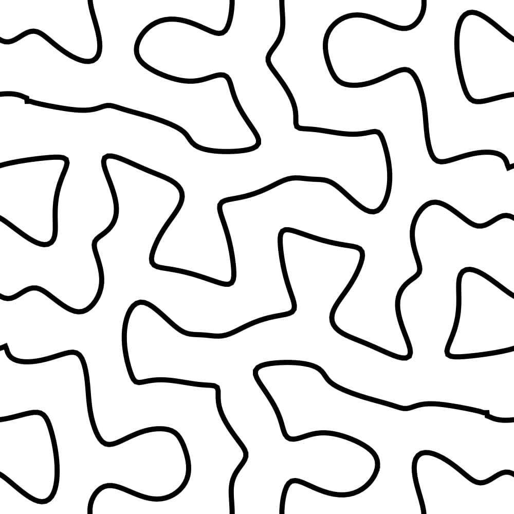
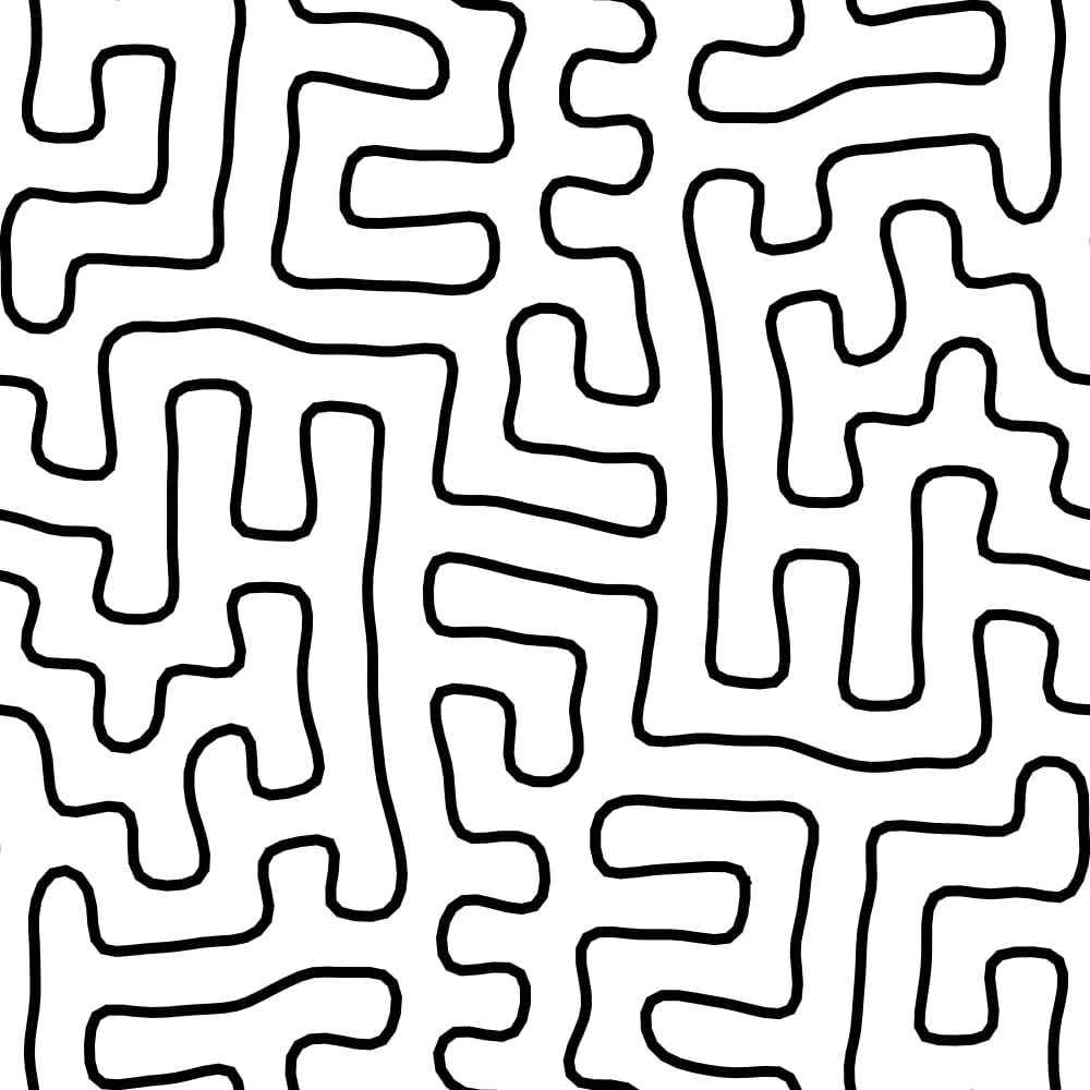
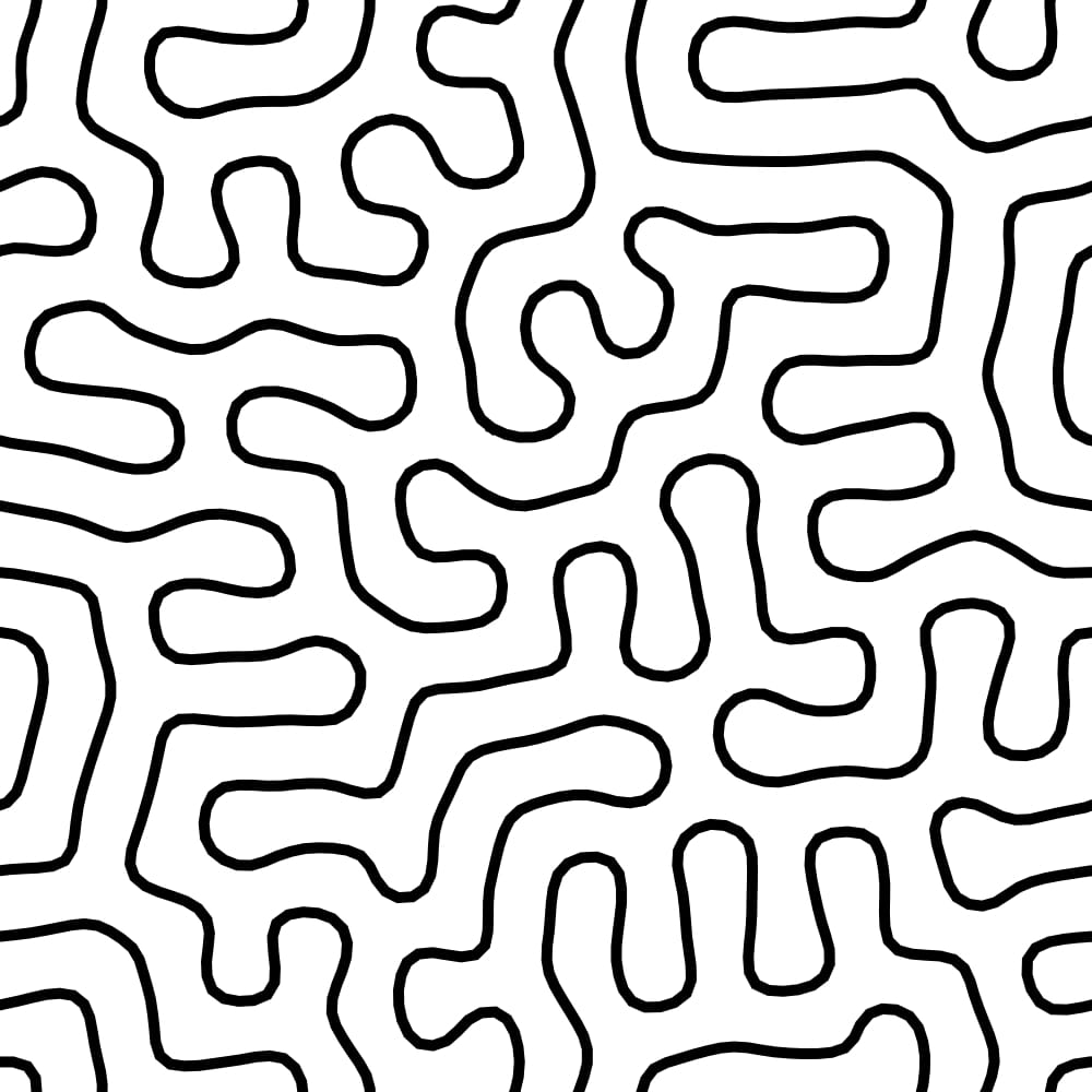
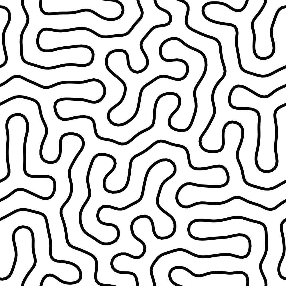
$\ell(\gamma)\approx 10.42$	$\ell(\gamma)\approx 16.96$	$\ell(\gamma)\approx 16.77$	$\ell(\gamma)\approx 16.63$	$\ell(\gamma)\approx 16.4$
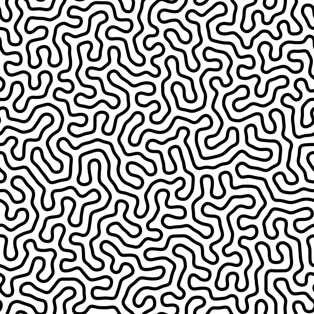
$\ell(\gamma)\approx 10.48$	$\ell(\gamma)\approx 20.83$	$\ell(\gamma)\approx 34.09$	$\ell(\gamma)\approx 33.52$	$\ell(\gamma)\approx 33.35$

Figure 2: Influence of $r$ on the local minimizer of (68) for the Lebesgue measure on $\mathbb{T}^{2}$. Column-wise we increase $r=16,32,64,128,256$ and row-wise we increase $L=2,4,8,16$, where $\lambda=0.2L^{-5}$ and $N=20L^{2}$. Note that the degree $r$ steers the resolution of the curves. It appears that the spacing of the curves is bounded by $r^{-1}$.

7.2 Quasi-optimal curves on special manifolds

In this subsection, we give numerical examples for $\mathbb{X}\in\{\mathbb{T}^{2},\mathbb{T}^{3},\mathbb{S}^{2},\operatorname*{SO}(3),\mathcal{G}_{2,4}\}$. Since the objective function in (68) is highly non-convex, the main problem is to find nearly optimal curves $\gamma_{L}\in\mathcal{P}_{L}^{\operatorname{{\lambda}-curv}}(\mathbb{X})$ for increasing $L$. Our heuristic is as follows:

• We start with a curve $\gamma_{L_{0}}\colon[0,1]\to\mathbb{X}$ of small length $\ell(\gamma)\approx L_{0}$ and solve the problem (68) for increasing $L_{i}=cL_{i-1}$, $c>1$, where we choose the parameters $N_{i}$, $\lambda_{i}$ and $r_{i}$ in dependence on $L_{i}$ as described in the previous subsection. In each step a local minimizer is computed using the CG method with 100 iterations. Then, the obtained minimizer $\gamma_{i}$ serves as the initial guess in the next step, which is obtained by inserting the midpoints.

• In case that the resulting curves $\gamma_{i}$ have non-constant speed, each is refined by increasing $\lambda_{i}$ and $N_{i}$. Then, the resulting problem is solved with the CG method and $\gamma_{i}$ as initialization. Details on the parameter choice are given in the according examples.

The following examples show that this recipe indeed enables us to compute “quasi-optimal” curves, meaning that the obtained minimizers have optimal decay in the discrepancy.

2d-Torus $\mathbb{T}^{2}$. In this example we illustrate how well a gray-valued image (considered as probability density) may be approximated by an almost constant speed curve. The original image of size 170x170 is depicted in the bottom-right corner of Fig. 4. Its Fourier coefficients $\hat{\mu}_{k_{1},k_{2}}$ are computed by a discrete Fourier transform (DFT) using the FFT algorithm and normalized appropriately. The kernel $K$ is given by (73) with $d=2$ and $s=3/2$.

We start with $N_{0}=96$ points on a circle given by the formula

$$x_{0,k}=\Bigl{(}\tfrac{1}{5}\cos(2\pi k/N_{0}),\tfrac{1}{5}\sin(2\pi k/N_{0})\Bigr{)},\qquad k=0,\dots,N_{0}.$$

Then, we apply our procedure for $i=0,\dots,11$ with parameters

$$L_{i}=0.97\cdot 2^{\frac{i+5}{2}},\quad\lambda_{i}=100\cdot L_{i}^{-5},\quad N_{i}=96\cdot 2^{i}\sim L_{i}^{2}\quad r_{i}=\lfloor 2^{\frac{i+11}{2}}\rfloor\sim L_{i},$$

chosen such that the length of the local minimizer $\gamma_{i}$ satisfies $\ell(\gamma_{i})\approx 2^{(i+5)/2}$ and the maximal speed is close to $L_{i}$.

To get nearly constant speed curves $\gamma_{i}$, see ii), we increase $\lambda_{i}$ by a factor of 100, $N_{i}$ by a factor of 2 and set $L_{i}\coloneqq 2^{(i+5)/2}$. Then, we apply the CG method with maximal 100 iterations and $i$ restarts. The results are depicted in Fig. 4. Note that the complexity for the evaluation of the function in (68) scales roughly as $N\sim L^{2}$. In Fig. 4 we observe that the decay-rate of the squared discrepancy $\mathscr{D}_{K}^{2}(\mu,\nu)$ in dependence on the Lipschitz constant $L$ matches indeed the theoretical findings of Theorem 4.9.

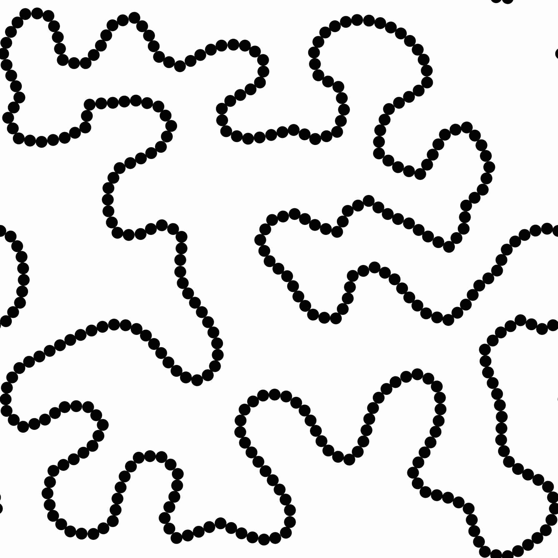
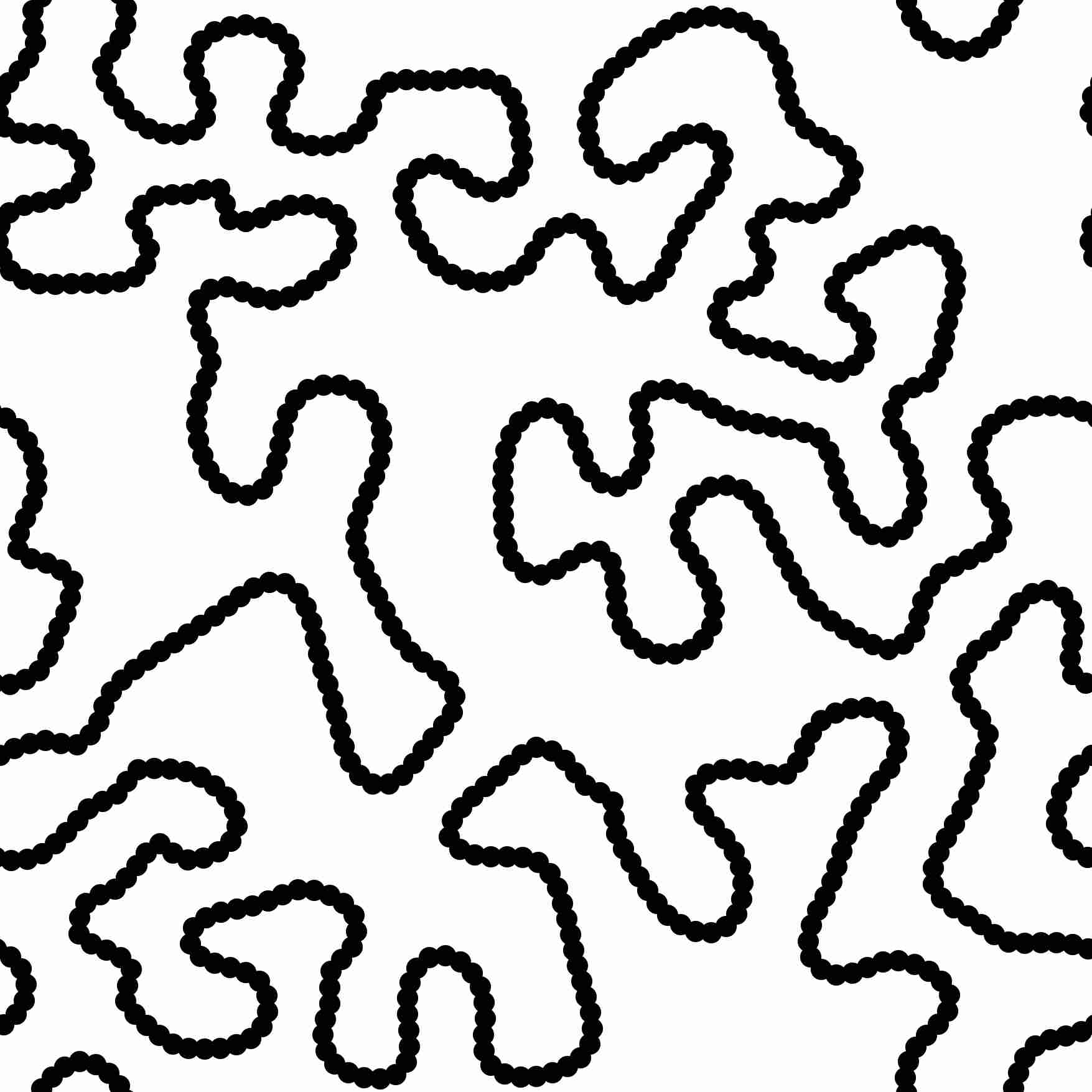
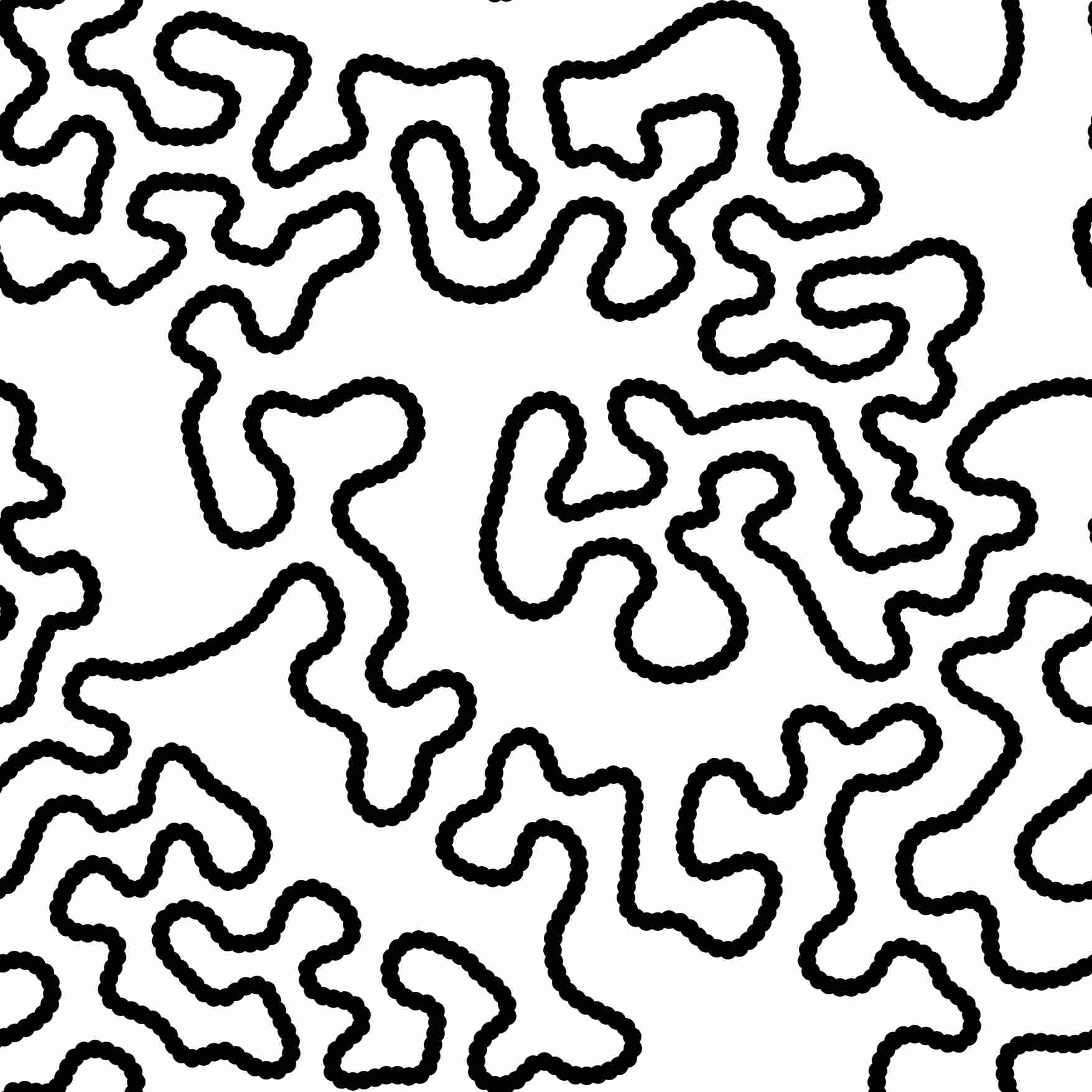
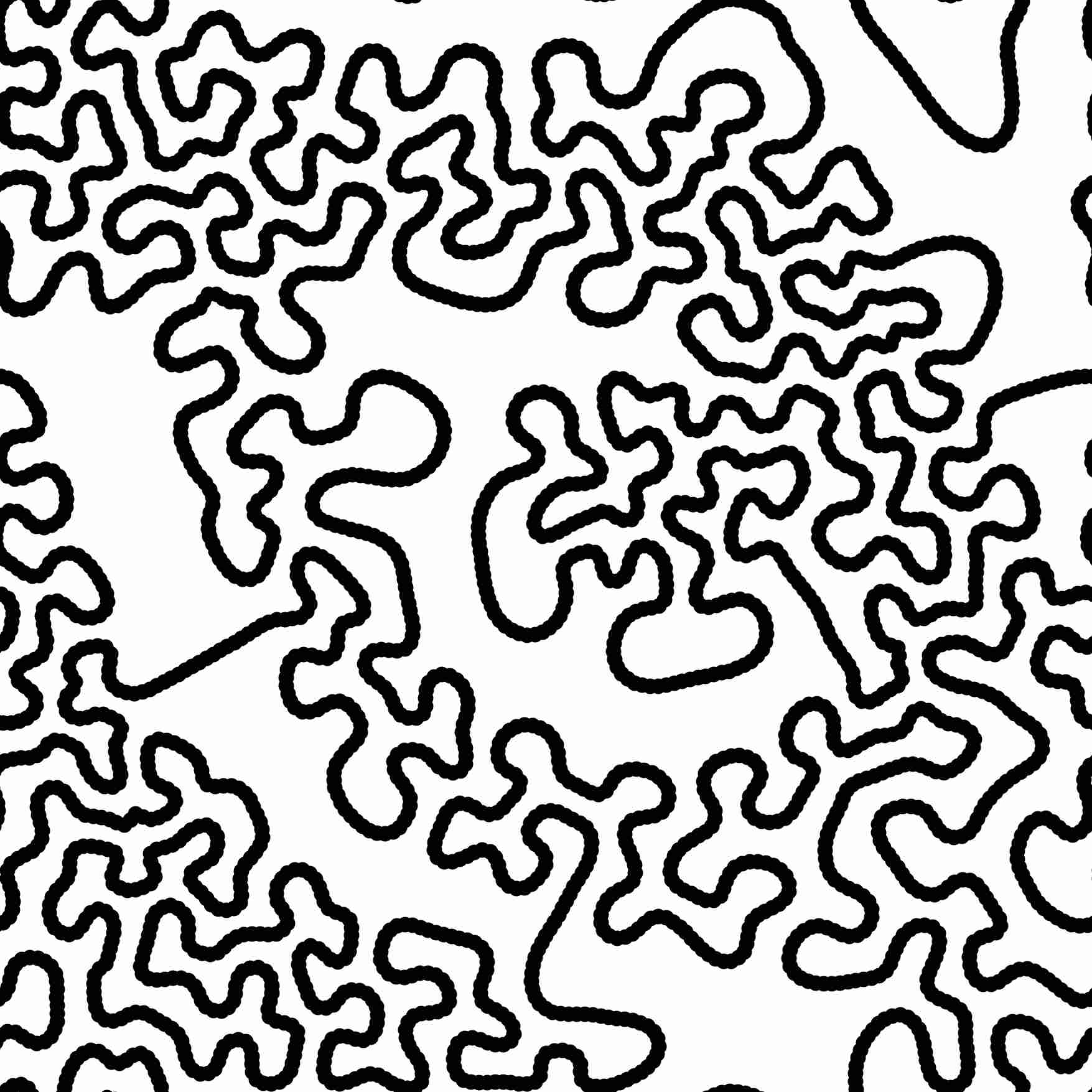
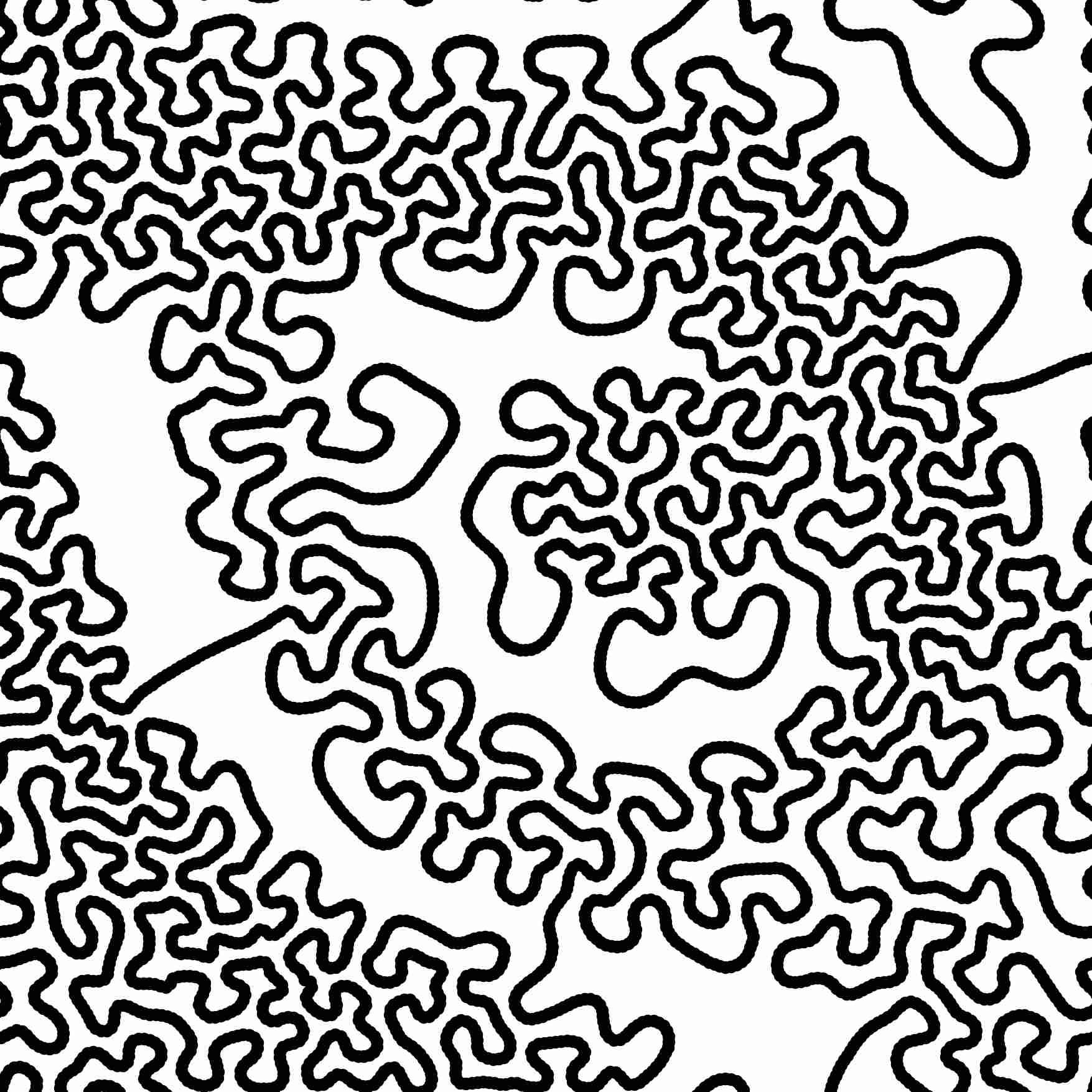
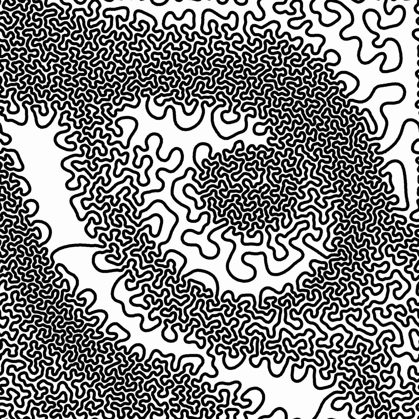
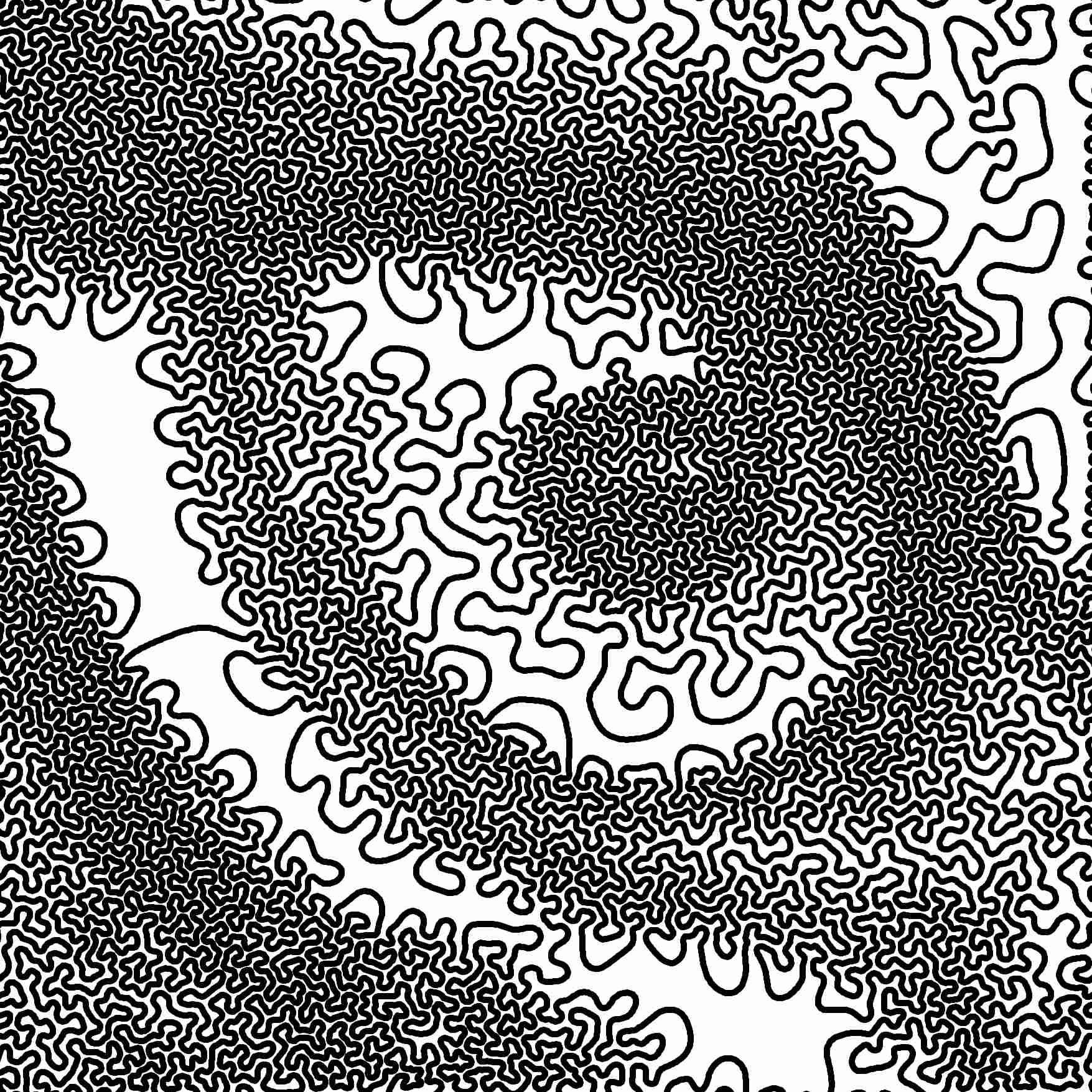
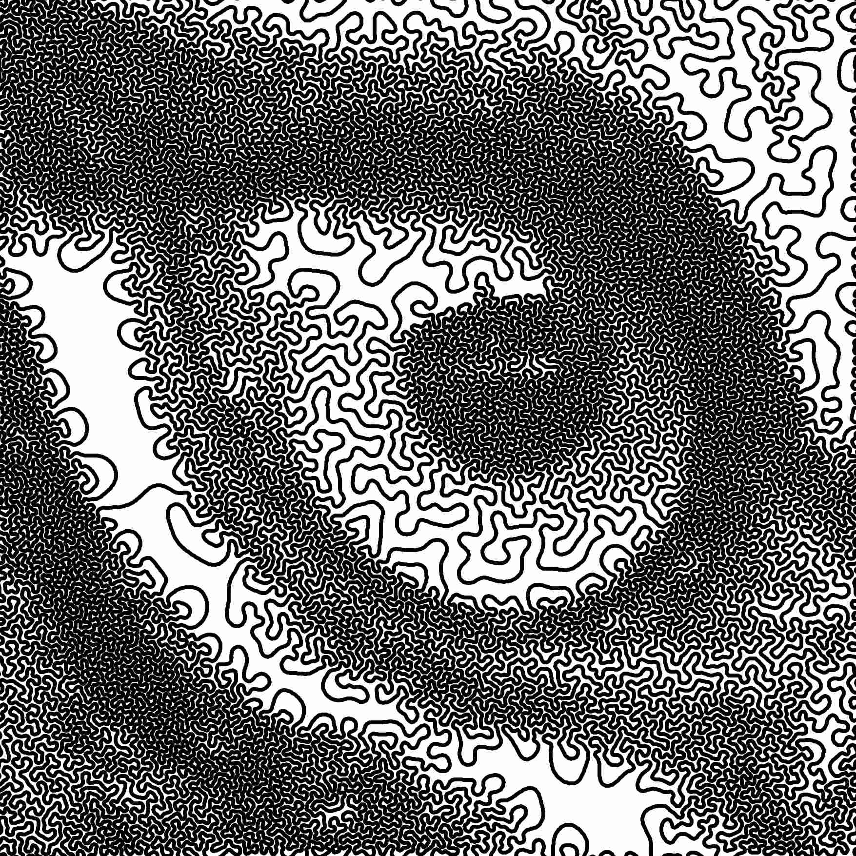
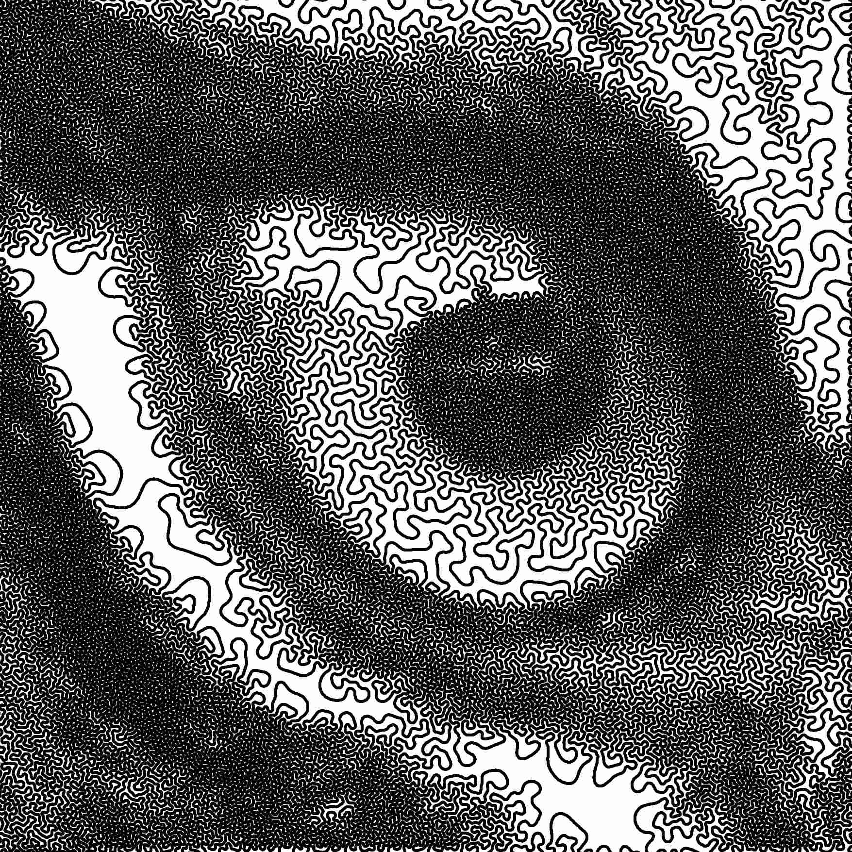
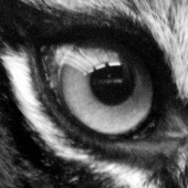
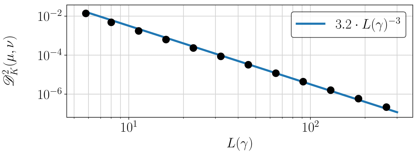
Figure 3: Local minimizers of (68) for the image at bottom right.

Figure 4: Squared discrepancy between the measure $\mu$ given by the image in Fig. 4 and the computed local minimizers (black dots) on $\mathbb{T}^{2}$ in log-scale. The blue line corresponds to the optimal decay-rate in Theorem 4.9.

3D-Torus $\mathbb{T}^{3}$. The aim of this example is two-fold. First, it shows that the algorithm works pretty well in three dimensions. Second, we are able to approximate any compact surface in the three-dimensional space by a curve. We construct a measure $\mu$ supported around a two-dimensional surface by taking samples from Spock’s head and placing small Gaussian peaks at the sampling points, i.e., the density is given for $x\in[-\tfrac{1}{2},\tfrac{1}{2}]$ by

$$\rho(x)\coloneqq c^{-1}\sum_{p\in S}\mathrm{e}^{-30000\|p-x\|_{2}^{2}},\qquad c\coloneqq\int_{[-\tfrac{1}{2},\tfrac{1}{2}]^{3}}\sum_{p\in S}\mathrm{e}^{-30000\|p-x\|_{2}^{2}}\,\mathrm{d}x,$$

where $S\subset[-\tfrac{1}{2},\tfrac{1}{2}]^{3}$ is the discrete sampling set. From a numerical point of view it holds $\mathrm{dim}(\textnormal{supp}(\mu))=2$. The Fourier coefficients are again computed by a DFT and the kernel $K$ is given by (73) with $d=3$ and $s=2$ so that $H_{K}=H^{2}(\mathbb{T}^{3})$.

We start with $N_{0}=100$ points on a smooth curve given by the formula

$$x_{0,k}=\Bigl{(}\tfrac{3}{10}\cos(2\pi k/N_{0}),\tfrac{3}{10}\sin(2\pi k/N_{0}),\tfrac{3}{10}\sin(4\pi k/N_{0})\Bigr{)},\qquad k=0,\dots,N_{0}.$$

Then, we apply our procedure for $i=0,\dots,8$ with parameters, cf. Remark 7.1,

$$L_{i}=2^{\frac{i+5}{2}},\quad\lambda_{i}=10\cdot L_{i}^{-5},\quad N_{i}=100\cdot 2^{i}\sim L_{i}^{2},\quad r_{i}=\lfloor 2^{\frac{i+5}{2}}\rfloor\sim L_{i}.$$

To get nearly constant speed curves $\gamma_{i}$, we increase $\lambda_{i}$ by a factor of 100, $N_{i}$ by a factor of 2 and set $L_{i}\coloneqq 2^{(i+6)/2}$. Then, we apply the CG method with maximal 100 iterations and one restart to the previously found curve $\gamma_{i}$. The results are illustrated in Fig. 6. Note that the complexity of the function evaluation in (68) scales roughly as $N^{3/2}\sim L^{3}$. In Fig. 6 we depict the squared discrepancy $\mathscr{D}_{K}^{2}(\mu,\nu)$ of the computed curves. For small Lipschitz constants, say $L(\gamma)\leq 50$, we observe a decrease of approximately $L(\gamma)^{-3}$, which matches the optimal decay-rate for measures supported on surfaces as discussed in Remark 4.13.

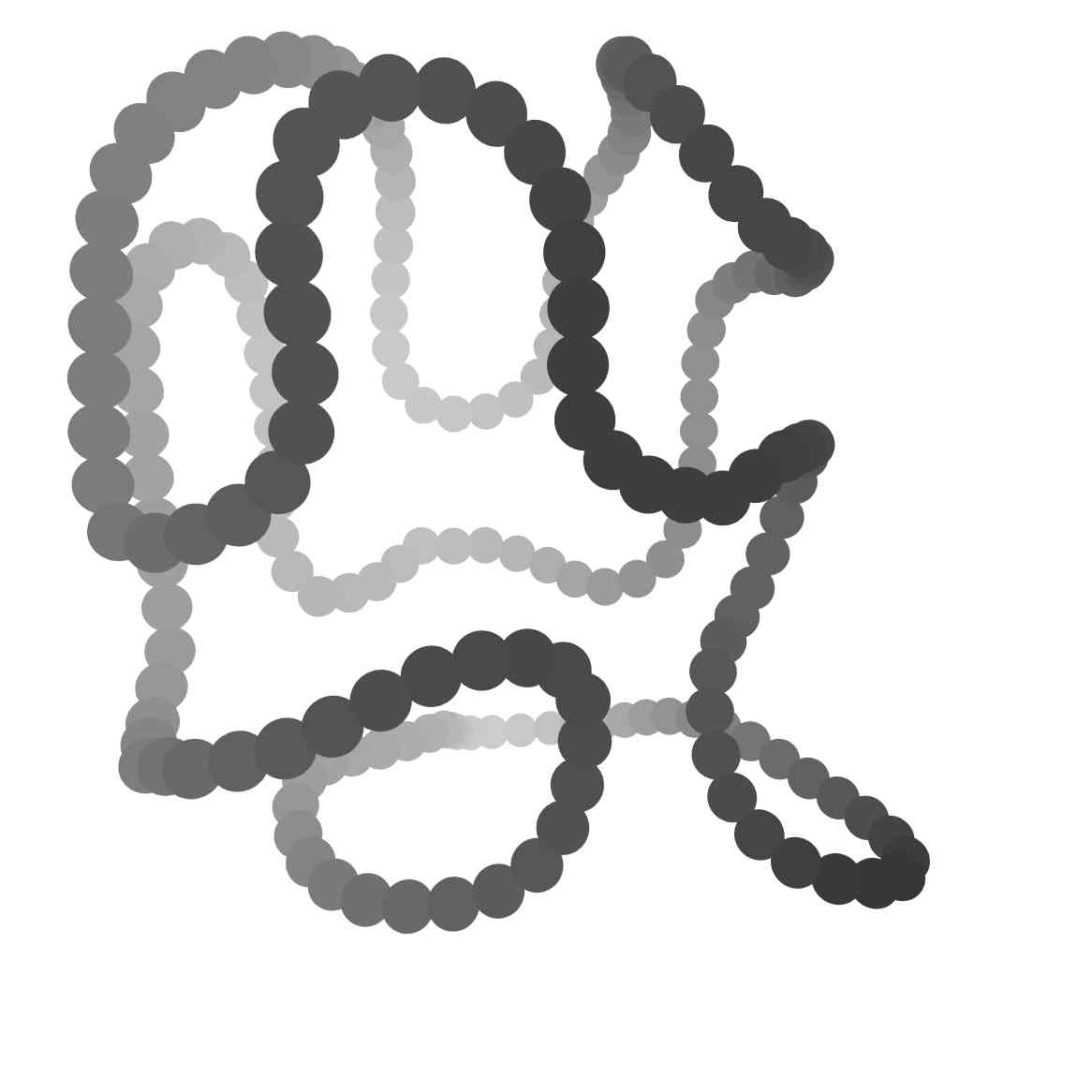
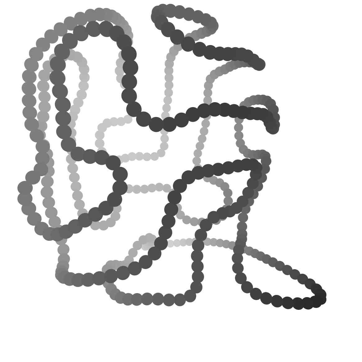
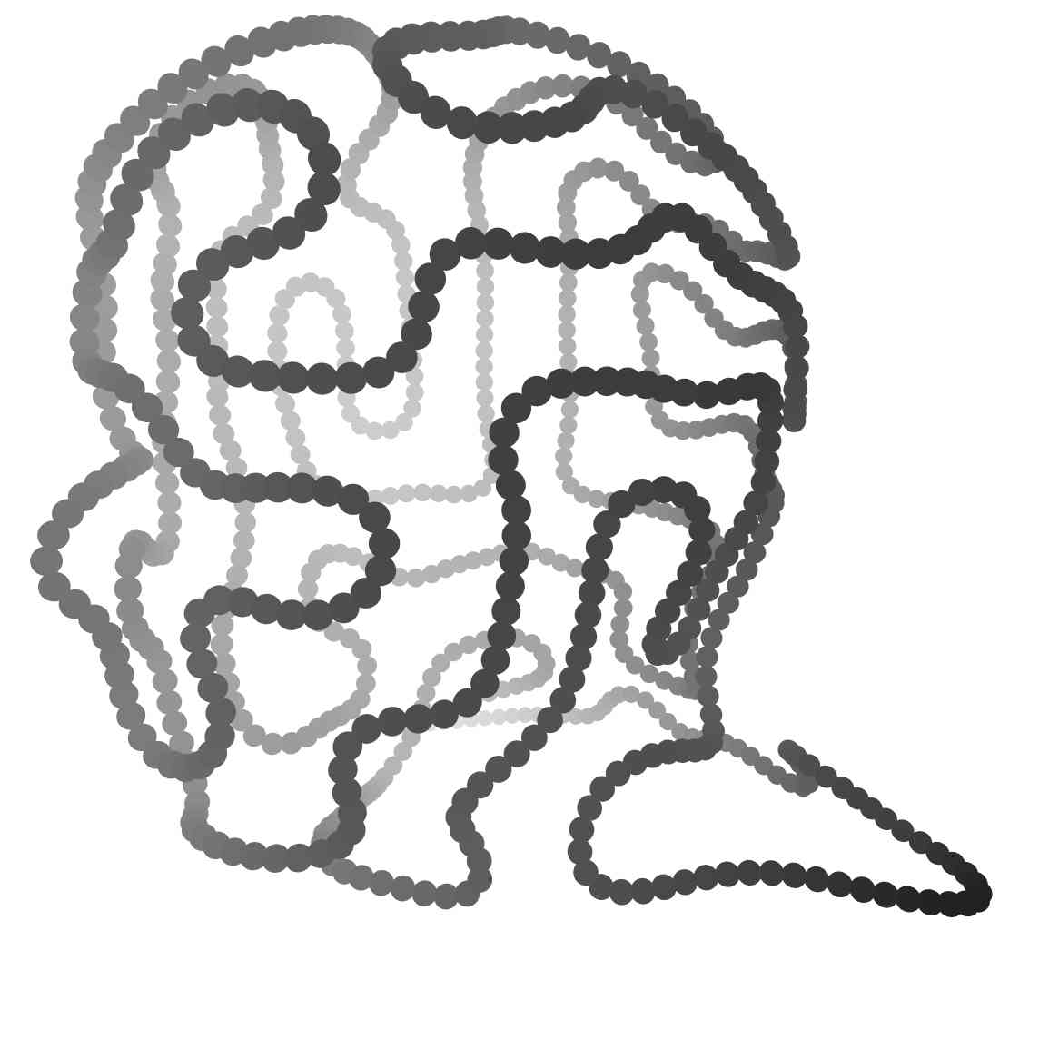
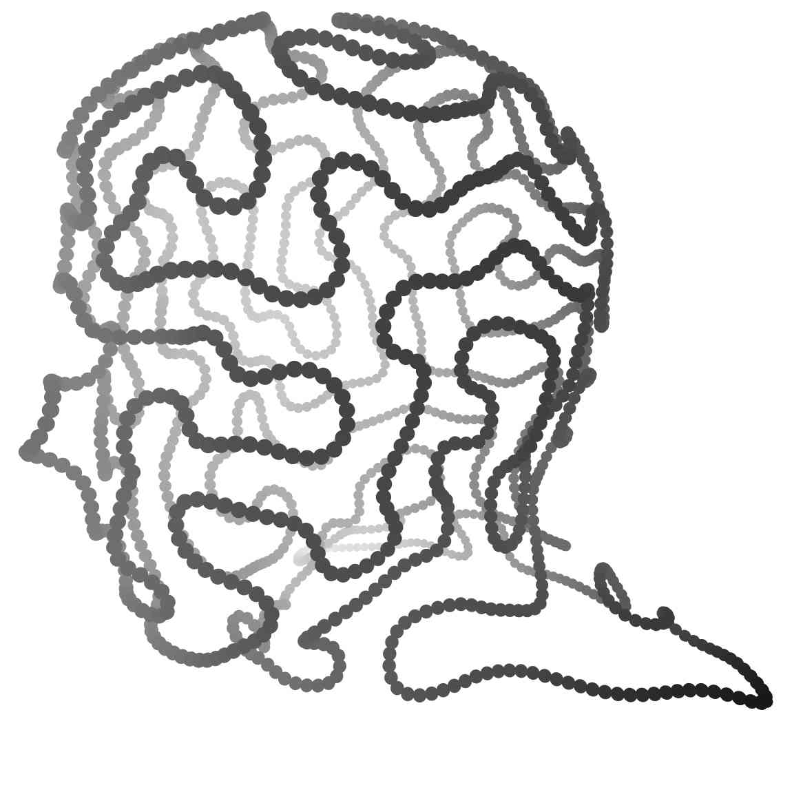
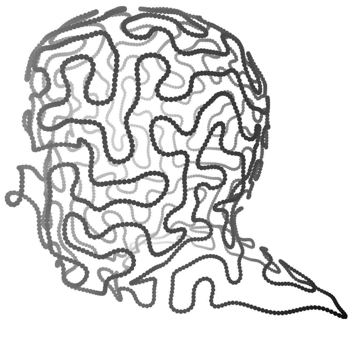
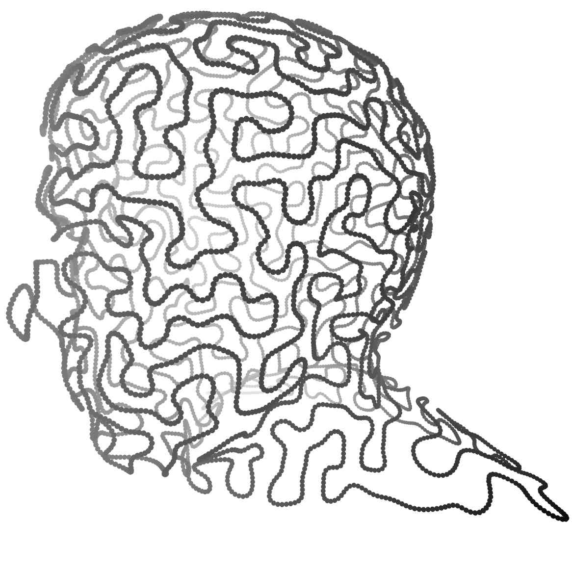
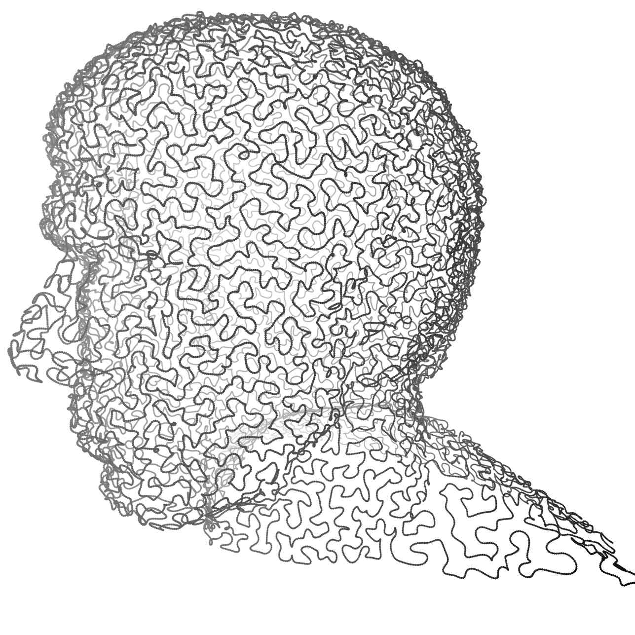
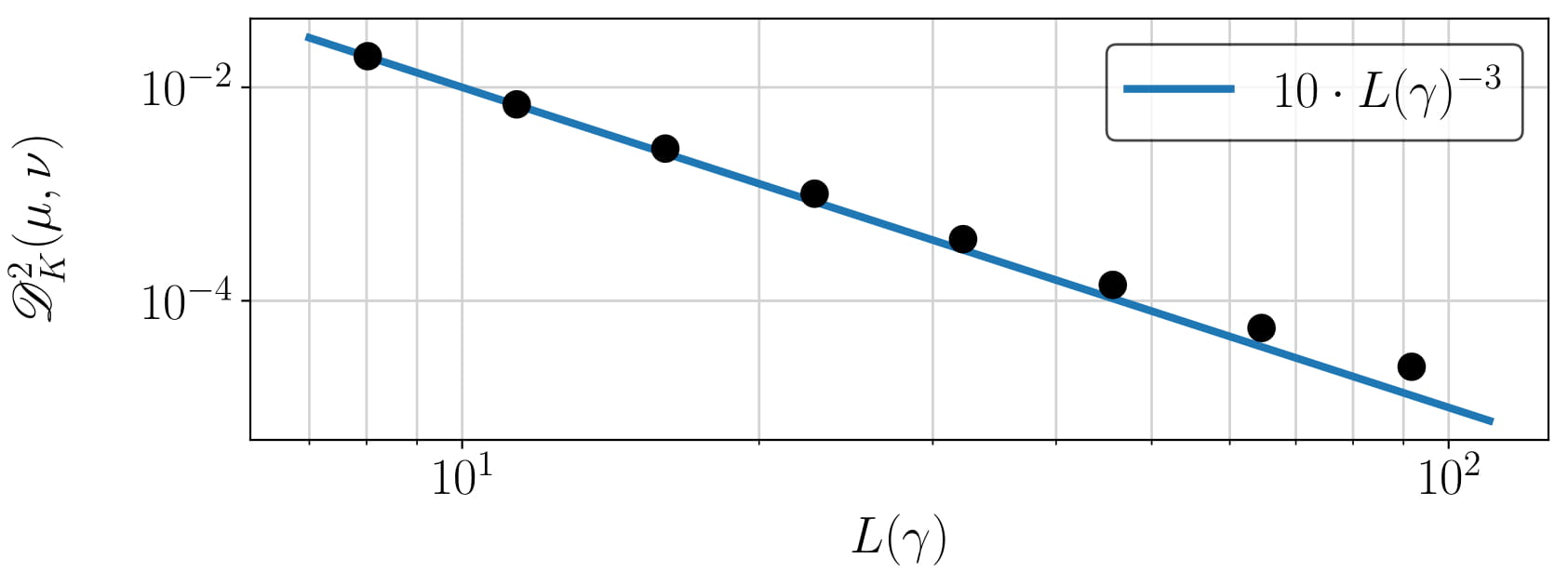
Figure 5: Local minimizers of (68) for a measure $\mu$ concentrated on a surface (head of Spock) in $\mathbb{T}^{3}$.

Figure 6: Squared discrepancy between the measure $\mu$ given by the surface in Fig. 6 and the computed local minimizers (black dots) on $\mathbb{T}^{3}$ in log-scale. The blue line corresponds to the optimal decay-rate in Theorem 4.9.

2-Sphere $\mathbb{S}^{2}$. Next, we approximate a gray-valued image on the sphere $\mathbb{S}^{2}$ by an almost constant speed curve. The image represents the earth’s elevation data provided by MATLAB, given by samples $\rho_{i,j}$, $i=1,\dots,180,\;j=1,\dots,360$, on the grid

$$x_{i,j}\coloneqq\Bigl{(}\sin\bigl{(}i\tfrac{\pi}{180}\bigr{)}\sin\bigl{(}j\tfrac{\pi}{180}\bigr{)},\sin\bigl{(}i\tfrac{\pi}{180}\bigr{)}\cos\bigl{(}j\tfrac{\pi}{180}\bigr{)},\cos\bigl{(}i\tfrac{\pi}{180}\bigr{)}\Bigr{)}.$$

The Fourier coefficients are computed by discretizing the Fourier integrals, i.e.,

$$\hat{\mu}_{k}^{m}\coloneqq\begin{cases}\frac{1}{180\cdot 360}\sum_{i=1}^{180}\sum_{j=1}^{360}\rho_{i,j}\overline{Y_{k}^{m}(x_{i,j})}\sin\bigl{(}i\tfrac{\pi}{180}\bigr{)},&1\leq k\leq 2m+1,m\leq 180,\\ 0,&\text{else},\end{cases}$$

followed by a normalization such that $\hat{\mu}_{0}^{0}=1$. The corresponding sums are efficiently computed by an adjoint non-equispaced fast spherical Fourier transform (NFSFT), see [68]. The kernel $K$ is given by (75). Similar to the previous examples, we apply our procedure for $i=0,\dots,12$ with parameters

$$L_{i}=9.7\cdot 2^{\frac{i}{2}},\quad\lambda_{i}=100\cdot L_{i}^{-5},\quad N_{i}=100\cdot 2^{i}\sim L_{i}^{2},\quad r_{i}=\lfloor L_{i}\rfloor\sim L_{i}.$$

To get nearly constant speed curves, we increase $\lambda_{i}$ by a factor of 100, $N_{i}$ by a factor of 2 and set $L_{i}\coloneqq L_{0}2^{i/2}$. Then, we apply the CG method with maximal 100 iterations and one restart to the previously constructed curves $\gamma_{i}$. The results for $i=6,8,10,12$ are depicted in Fig. 8. Note that the complexity of the function evaluation in (68) scales roughly as $N\sim L^{2}$. In Fig. 8 we observe that the decay-rate of the squared discrepancy $\mathscr{D}_{K}^{2}(\mu,\nu)$ in dependence on the Lipschitz constant matches indeed the theoretical findings in Theorem 4.10.

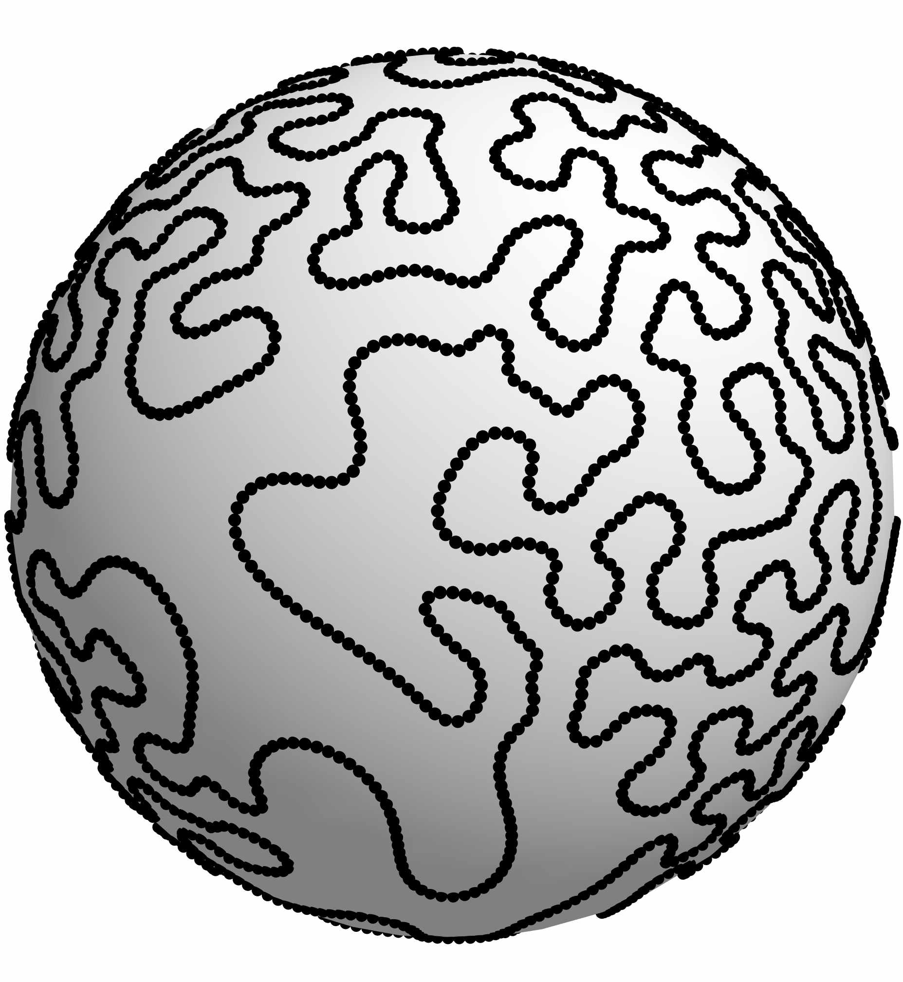
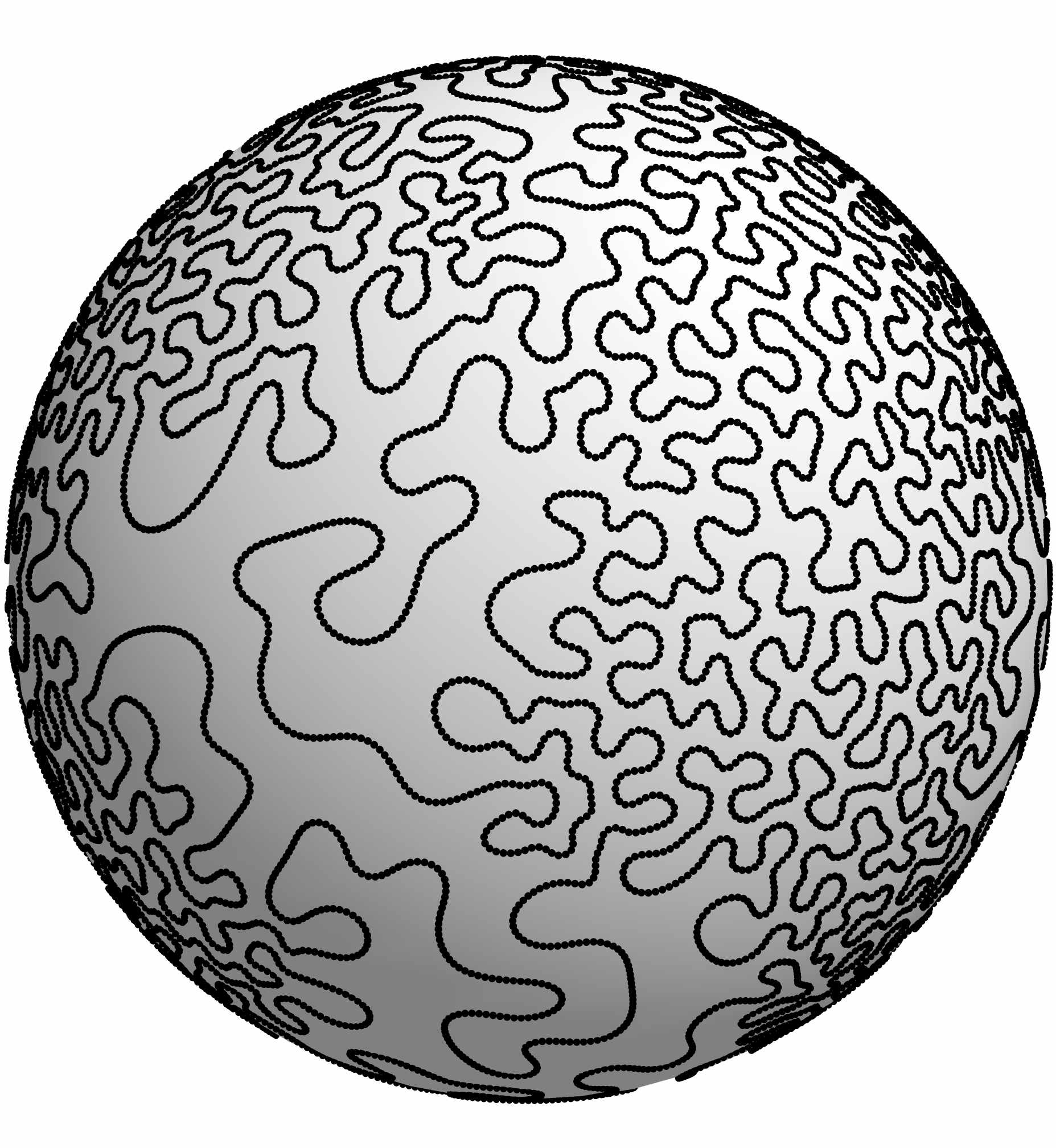
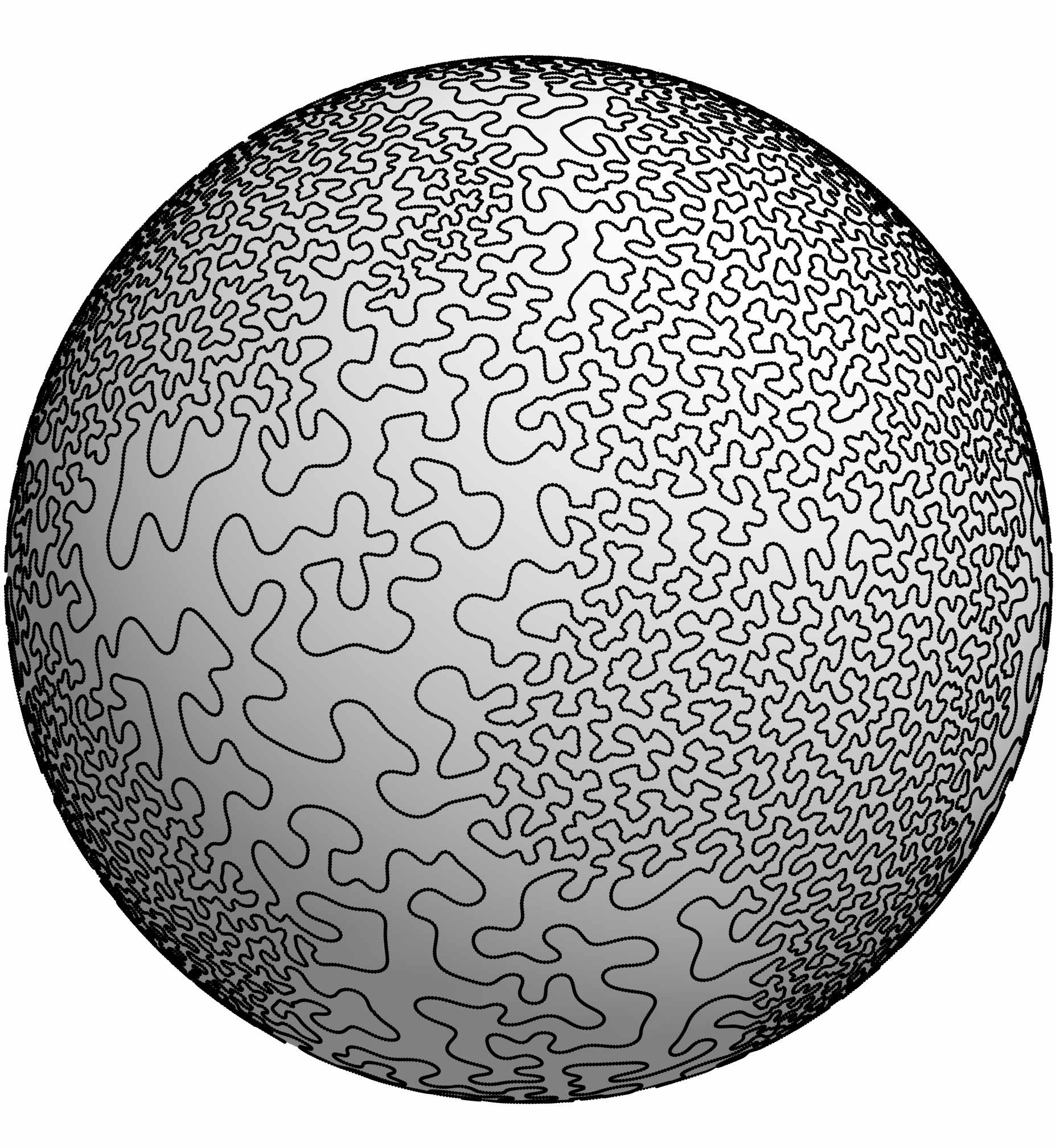
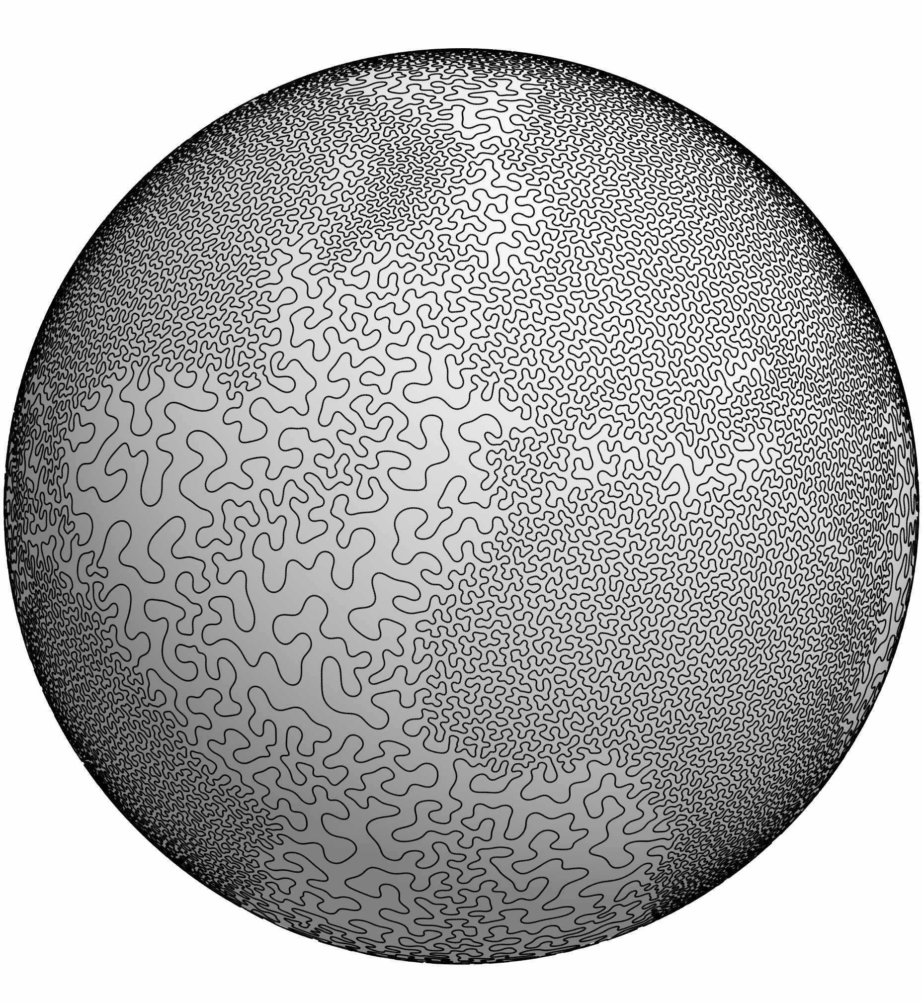
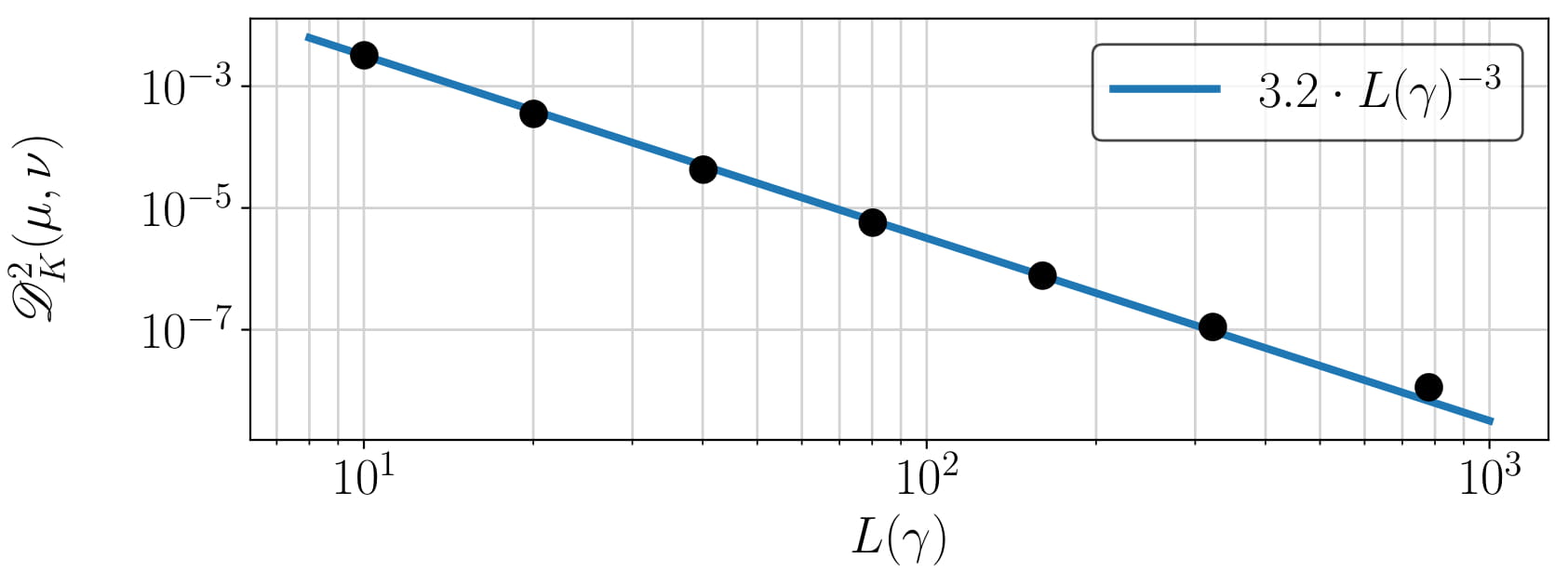
Figure 7: Local minimizers of (68) for $\mu$ given by the earth’s elevation data on the sphere $\mathbb{S}^{2}$.

Figure 8: Squared discrepancy between the measure $\mu$ and the computed local minimizers (black dots) in log-scale. The blue line corresponds to the optimal decay-rate in Theorem 4.10.

3D-Rotations $\operatorname*{SO}(3)$. There are several possibilities to parameterize the rotation group $\operatorname*{SO}(3)$. We apply those by Euler angles and an axis-angle representation for visualization. Euler angles $(\varphi_{1},\theta,\varphi_{2})\in[0,2\pi)\times[0,\pi]\times[0,2\pi)$ correspond to rotations $\mathrm{Rot}(\varphi_{1},\theta,\varphi_{2})$ in $\operatorname*{SO}(3)$ that are the successive rotations around the axes $e_{3},e_{2},e_{3}$ by the respective angles. Then, the Haar measure of $\operatorname*{SO}(3)$ is determined by

$$\,\mathrm{d}\mu_{\mathrm{SO(3)}}(\varphi_{1},\theta,\varphi_{2})=\tfrac{1}{8\pi^{2}}\sin(\theta)\,\mathrm{d}\varphi_{1}\,\mathrm{d}\theta\,\mathrm{d}\varphi_{2}.$$

We are interested in the full three-dimensional doughnut

$$D=\bigl{\{}\mathrm{Rot}(\varphi_{1},\theta,\varphi_{2})\;:\;0\leq\theta\leq\tfrac{\pi}{2},\;0\leq\varphi_{1},\varphi_{2}\leq 2\pi\bigr{\}}\subset\mathrm{SO(3)}.$$

Next, we want to approximate the Haar measure $\mu=\mu_{D}$ restricted to $D$, i.e., with normalization we consider the measure defined for $f\in C(\operatorname*{SO}(3))$ by

$$\int_{\mathrm{SO(3)}}f\,\mathrm{d}\mu_{D}=\frac{1}{4\pi^{2}}\int_{0}^{2\pi}\int_{0}^{\frac{\pi}{2}}\int_{0}^{2\pi}f(\varphi_{1},\theta,\varphi_{2})\sin(\theta)\,\mathrm{d}\varphi_{1}\,\mathrm{d}\theta\,\mathrm{d}\varphi_{2}.$$

The Fourier coefficients of $\mu_{D}$ can be explicitly computed by

$$\hat{\mu}_{l,l^{\prime}}^{k}=\begin{cases}P_{k-1}(0)-P_{k+1}(0),&l,l^{\prime}=0,\;k\geq 0,\\ 0,&l,l^{\prime}\neq 0,\end{cases}$$

where $P_{k}$ are the Legendre polynomials. The kernel $K$ is given by (77) with $d=3$ and $s=2$. For $i=0,\dots,8$ the parameters are chosen as

$$L_{i}=0.93\cdot 2^{\frac{2i+12}{3}},\quad\lambda_{i}=10\cdot L_{i}^{-4},\quad N_{i}=64\cdot 2^{i}\sim L_{i}^{2},\quad r_{i}=\lfloor 2^{\frac{i+9}{3}}\rfloor\sim L_{i}^{\frac{1}{2}}.$$

Here, we use a CG method with 100 iterations and one restart. Step ii) appears to be not necessary. Note that the complexity for the function evaluations in (68) scales roughly as $N\sim L^{3/2}$.

The constructed curves are illustrated in Fig. 10, where we utilized the following visualization: Every rotation $R(\alpha,r)\in\operatorname*{SO}(3)$ is determined by a rotation axis $r=(r_{1},r_{2},r_{3})\in\mathbb{S}^{2}$ and a rotation angle $\alpha\in[0,\pi]$, i.e.,

$$R(\alpha,r)x=r(r^{\mathrm{T}}x)+\cos(\alpha)\left((r\times x)\times r\right)+\sin(\alpha)(r\times x).$$

Setting $q\coloneqq(\cos(\tfrac{\alpha}{2}),\sin(\tfrac{\alpha}{2})r)\in\mathbb{S}^{3}$ with $r\in\mathbb{S}^{2}$ and $\alpha\in[0,2\pi]$, see (40), we observe that the same rotation is generated by $-q=(\cos(\tfrac{2\pi-\alpha}{2}),\sin(\tfrac{2\pi-\alpha}{2}(-r))\in\mathbb{S}^{3}$, in other words $\operatorname*{SO}(3)\cong\mathbb{S}^{3}/\{\pm 1\}$. Then, by applying the stereographic projection $\pi(q)=(q_{2},q_{3},q_{4})/(1+q_{1})$, we map the upper hemisphere onto the three dimensional unit ball. Note that the equatorial plane of $\mathbb{S}^{3}$ is mapped onto the sphere $\mathbb{S}^{2}$, hence on the surface of the ball antipodal points have to be identified. In other words, the rotation $R(\alpha,r)$ is plotted as the point

$$\pi(q)=\frac{\sin\bigl{(}\tfrac{\alpha}{2}\bigr{)}}{1+\cos\bigl{(}\tfrac{\alpha}{2}\bigr{)}}r=\tan\bigl{(}\tfrac{\alpha}{4}\bigr{)}r\in\mathbb{R}^{3}.$$

In Fig. 10 we observe that the decay-rate of $\mathscr{D}_{K}^{2}(\mu,\nu)$ in dependence on the Lipschitz constant $L$ matches the theoretical findings in Corollary 4.7.

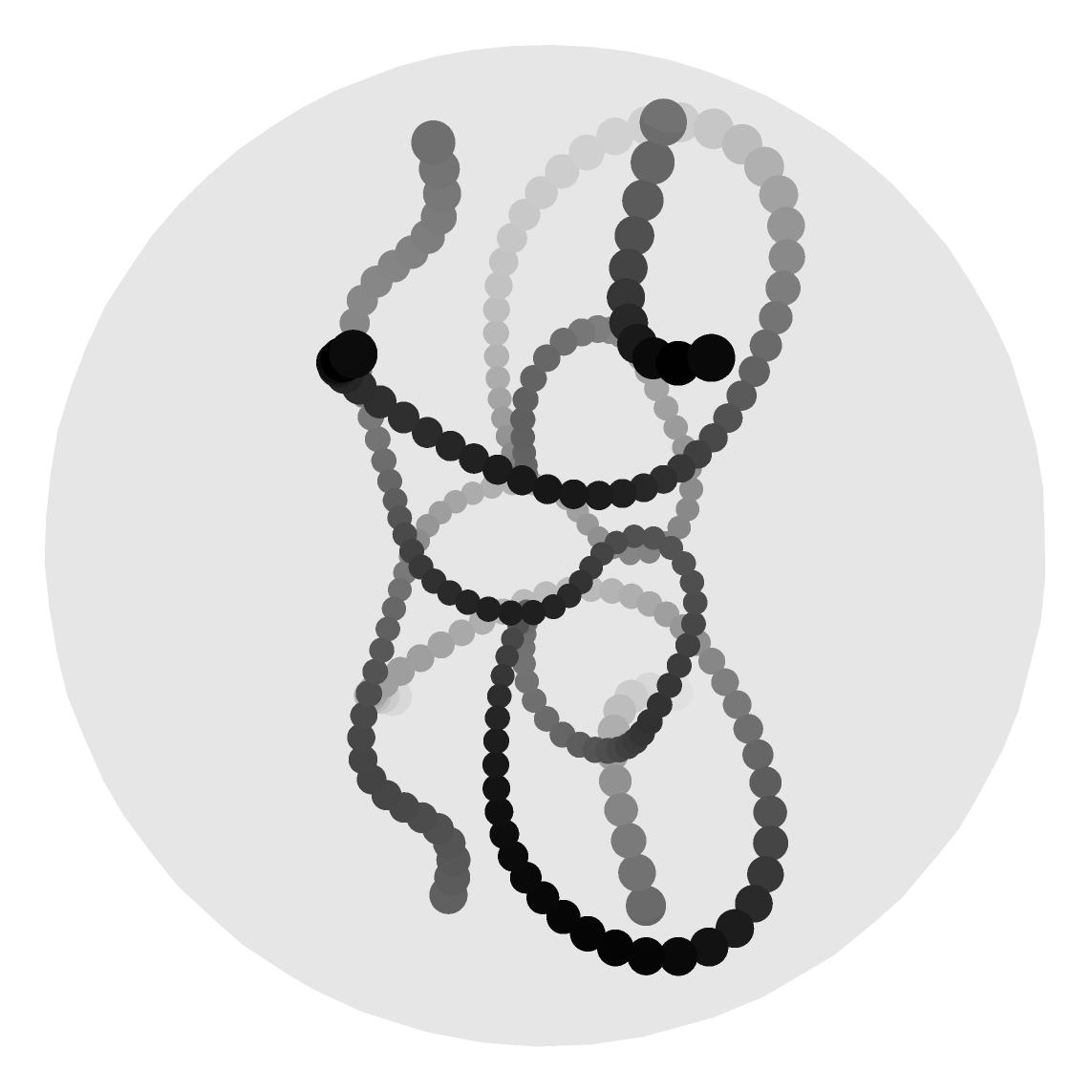
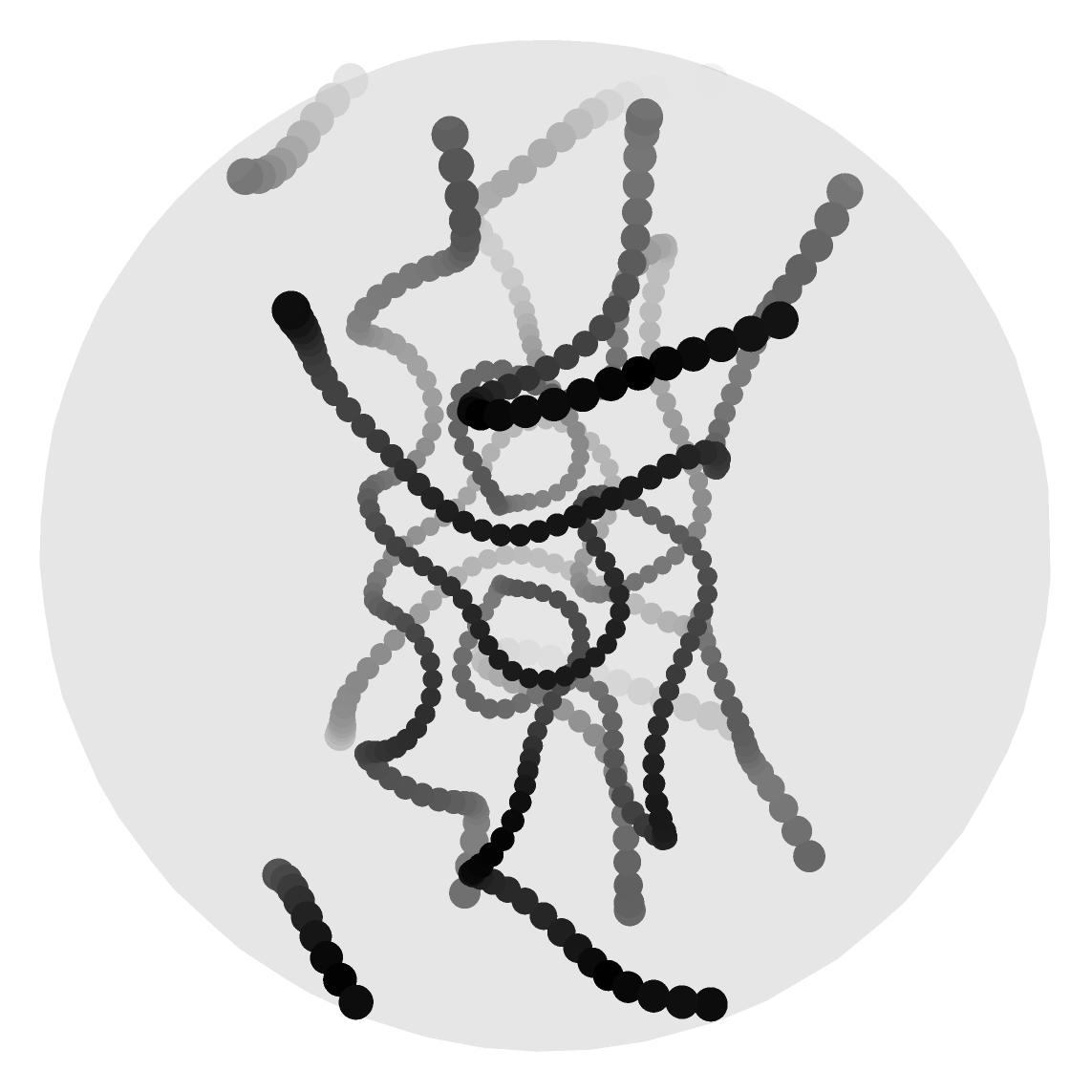
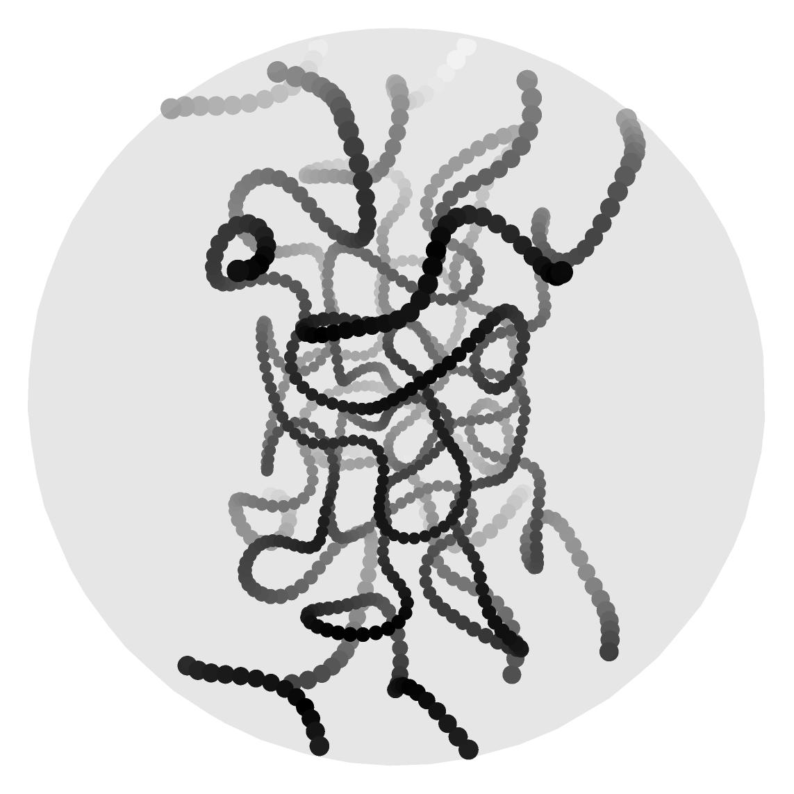
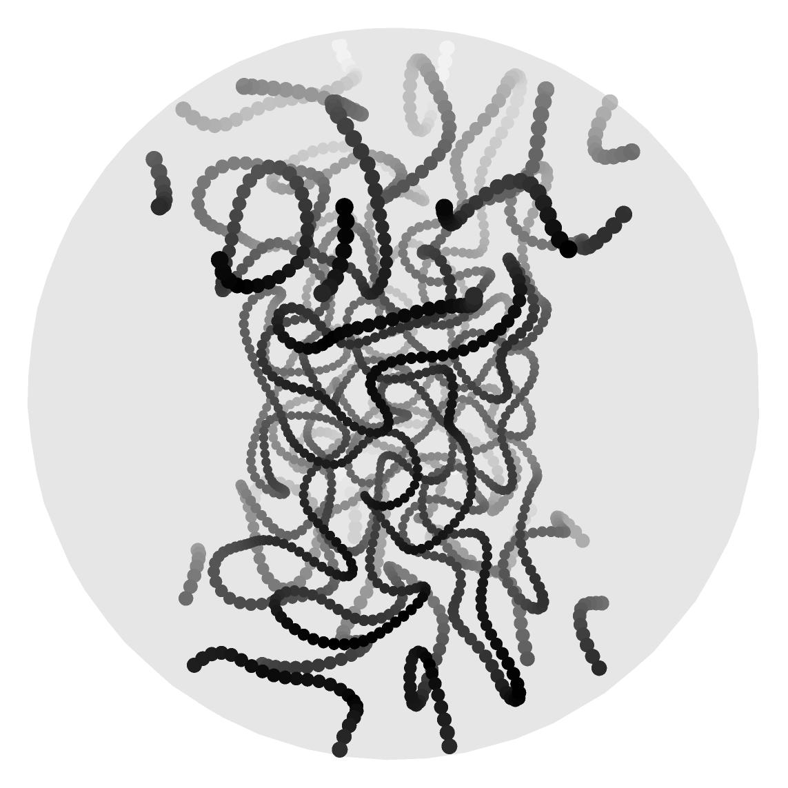
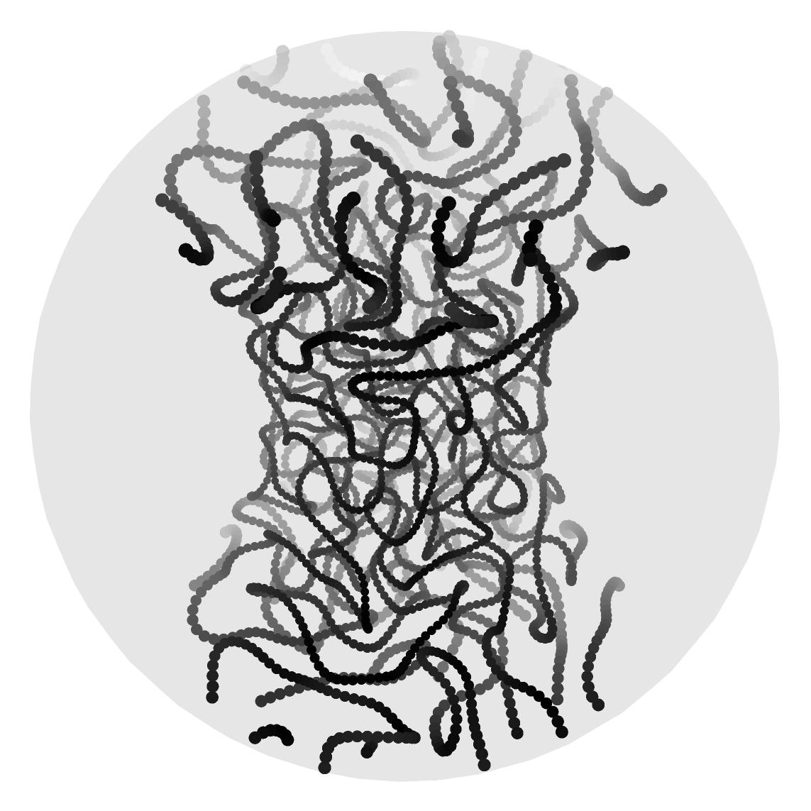
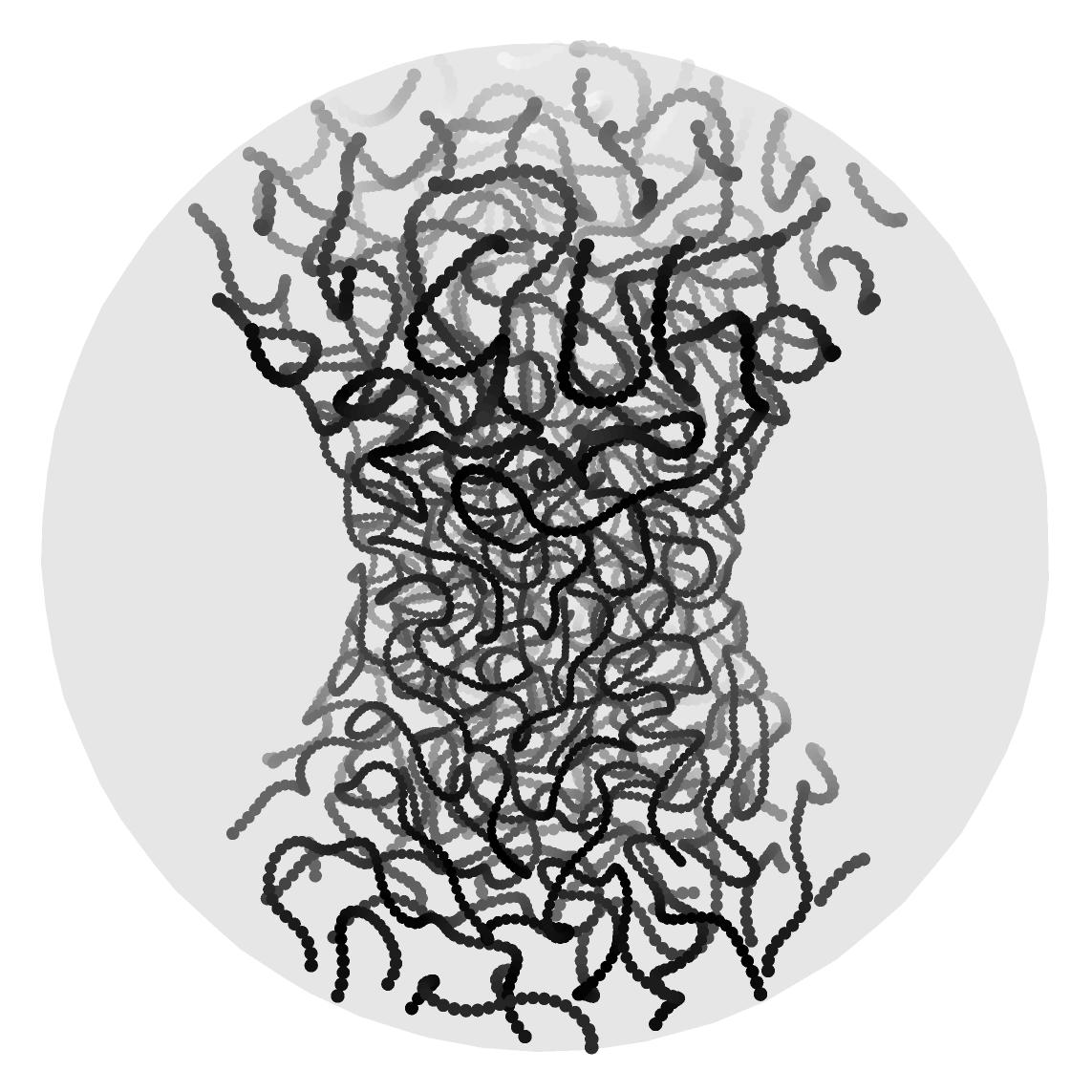
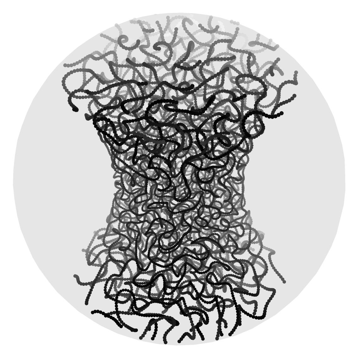
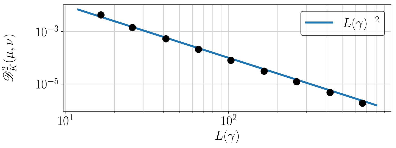
Figure 9: Local minimizers of (68) for Haar measure $\mu_{D}$ of three-dimensional doughnut $D$ in the rotation group $\mathrm{SO(3)}$. Color scheme for better visibility of 3D structure.

Figure 10: Squared discrepancy between the measure $\mu_{D}$ and the computed local minimizers (black dots) in log-scale. The blue line corresponds to the optimal decay-rate in Corollary 4.7.

The $4$-dimensional Grassmannian $\mathcal{G}_{2,4}$. Here, we aim to approximate the Haar measure of the Grassmannian $\mathcal{G}_{2,4}$ by a curve of almost constant speed. As this curve samples the space $\mathcal{G}_{2,4}$ quite evenly, it could be used for the grand tour, a technique to analyze high-dimensional data by their projections onto two-dimensional subspaces, cf. [5].

The kernel $K$ of the Haar measure is given by (80) and the Fourier coefficients are given by $\hat{\mu}_{m,m^{\prime}}^{k,k^{\prime}}=\delta_{m,0}\delta_{m^{\prime},0}\delta_{k,0}\delta_{k^{\prime},0}$. For $i=0,\dots,8$ the parameters are chosen as

$$L_{i}=0.91\cdot 2^{\frac{3i+16}{4}},\,\,\,\lambda_{i}=100\cdot L_{i}^{-\frac{11}{3}},\,\,\,N_{i}=128\cdot 2^{i}\sim L_{i}^{2},\,\,\,r_{i}=\lfloor 2^{\frac{3i+16}{12}}\rfloor+1\sim L_{i}^{\frac{1}{3}}.$$

Here, we use a CG method with 100 iterations and one restart. Our experiments suggest that step ii) is not necessary. Note that the complexity for the function evaluation in (68) scales roughly as $N\sim L^{3/2}$.

The computed curves are illustrated in Fig. 12, where we use the following visualization. By Remark A.1, there exists an isometric one-to-one mapping $P\colon\mathbb{S}^{2}\times\mathbb{S}^{2}/\{\pm 1\}\to\operatorname{\mathcal{G}}_{2,4}$. Using this relation, we plot the point $P(u,v)\in\mathcal{G}_{2,4}$ by two antipodal points $z_{1}=u+v,\,z_{2}=-u-v\in\mathbb{R}^{3}$ together with the RGB color-coded vectors $\pm u$. More precisely, $R=(1\mp u_{1})/2$, $G=(1\mp u_{2})/2$, $B=(1\mp u_{3})/2$. This means a curve $\gamma(t)\in\mathcal{G}_{2,4}$ only intersects itself if the corresponding curve $z(t)\in\mathbb{R}^{3}$ intersects and has the same colors at the intersection point. In Fig. 12 we observe that the decay-rate of the squared discrepancy $\mathscr{D}_{K}^{2}(\mu,\nu)$ in dependence on the Lipschitz constant $L$ matches indeed the theoretical findings in Theorem 4.11.

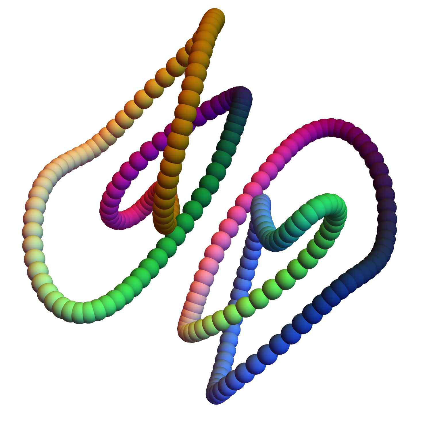
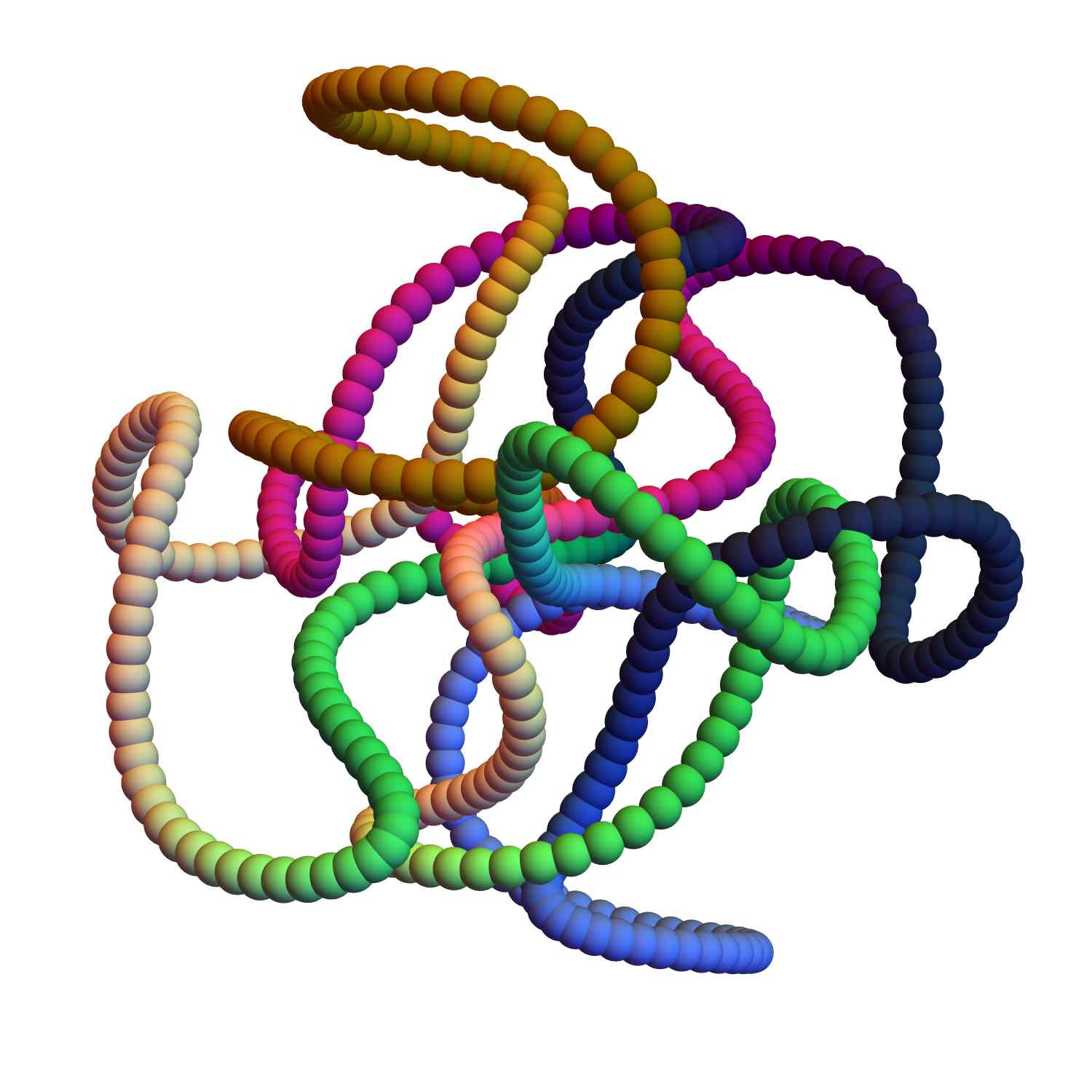
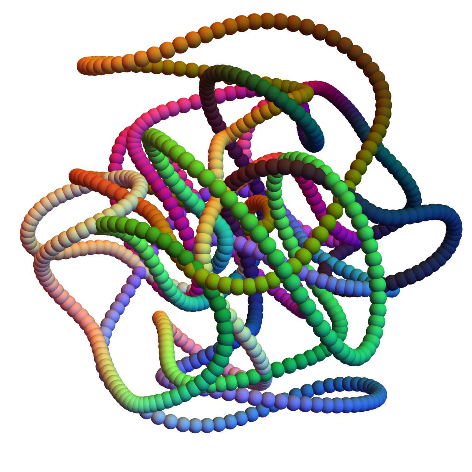
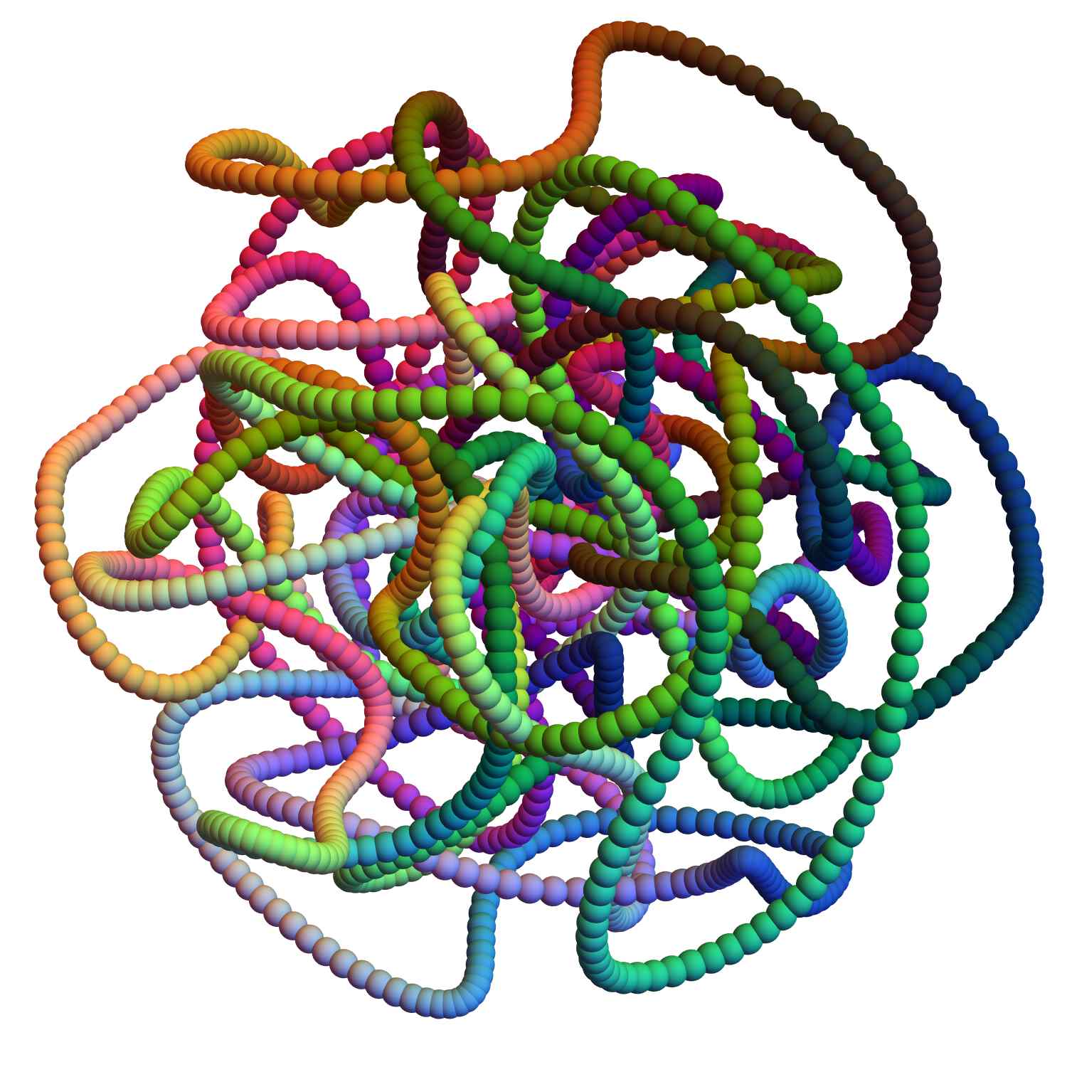
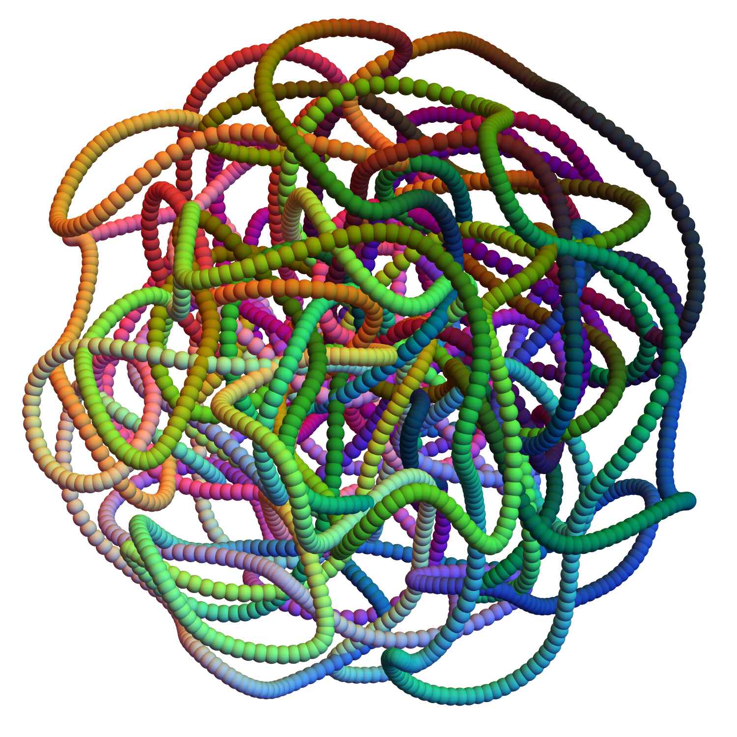
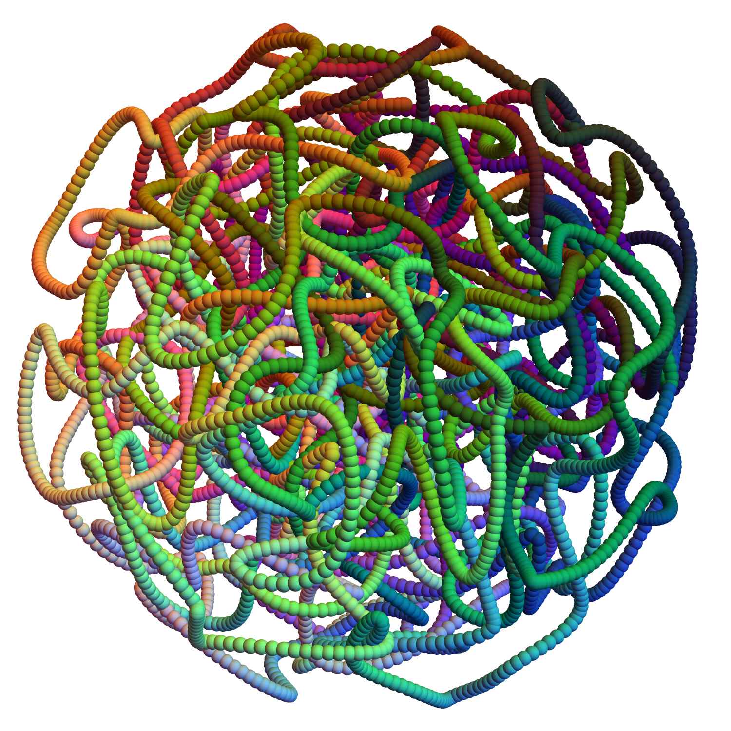
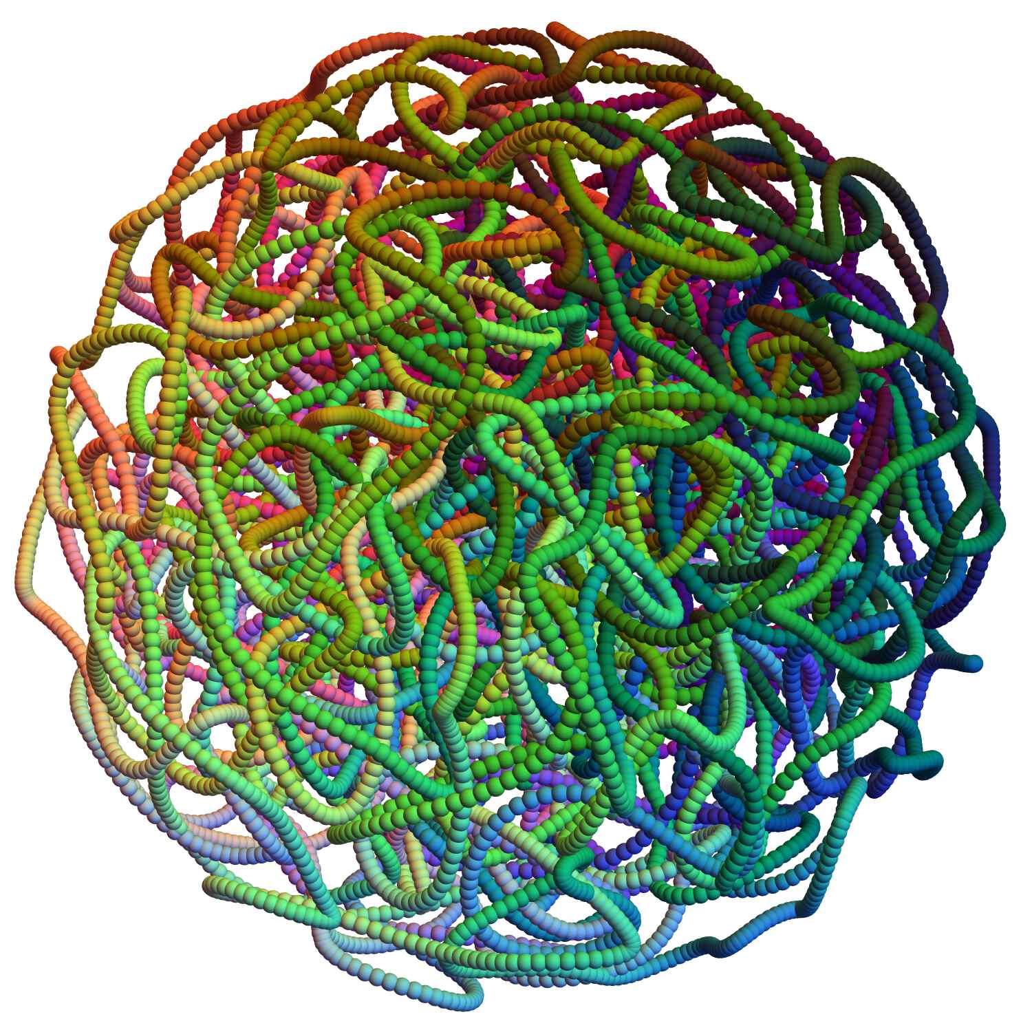
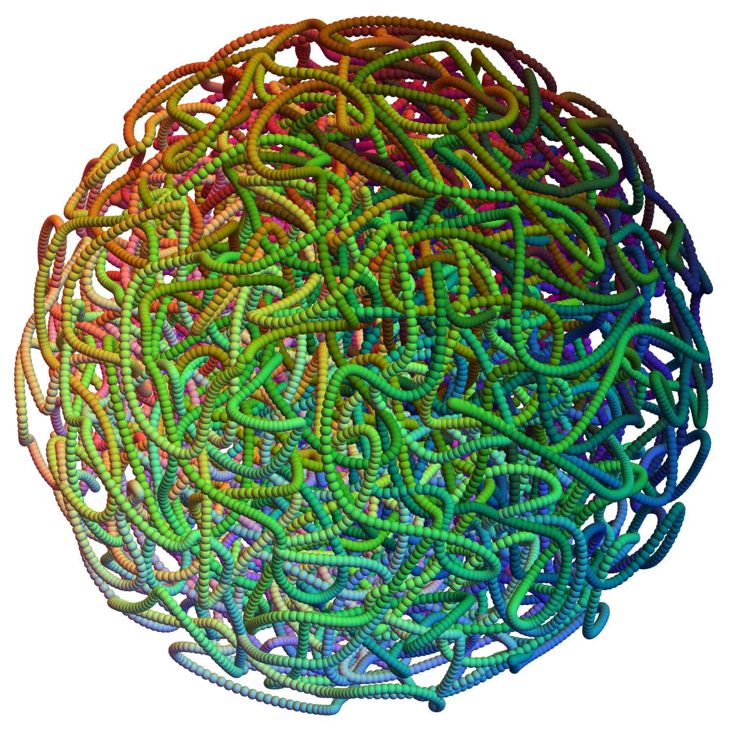
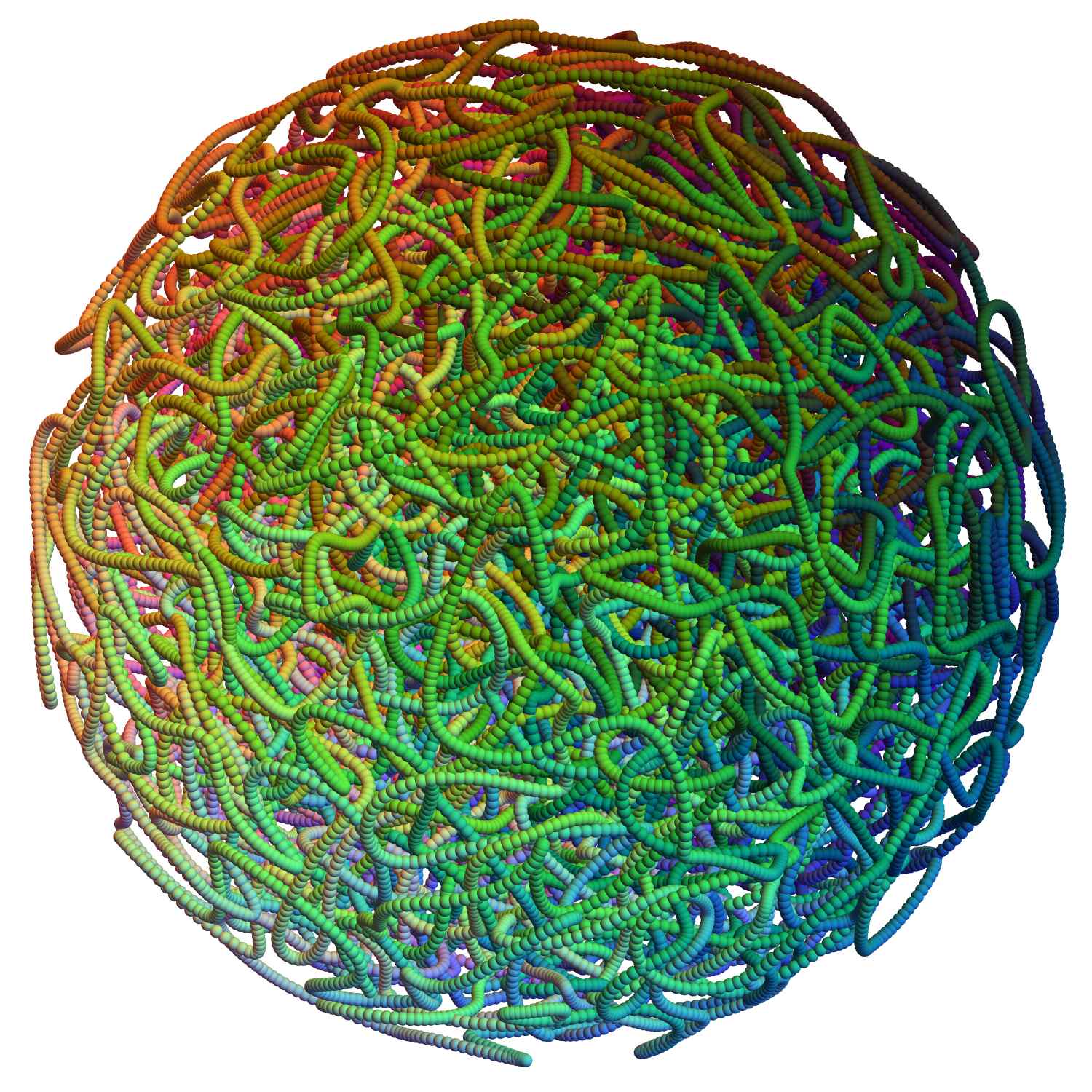
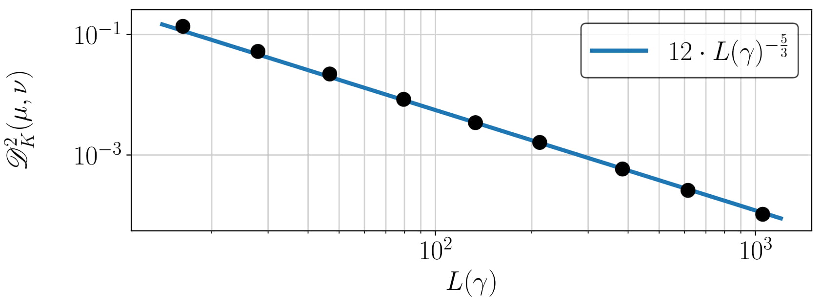
Figure 11: Local minimizers of (68) for the Haar measure of the Grassmannian $\mathcal{G}_{2,4}$.

Figure 12: The squared discrepancy between the Haar measure $\mu$ and the computed local minimizers (black dots) in log-scale. Here, the blue line corresponds to the optimal decay-rate, cf. Theorem 4.11.

8 Conclusions

In this chapter, we provided approximation results for general probability measures on compact Ahlfors $d$-regular metric spaces $\mathbb{X}$ by

• measures supported on continuous curves of finite length, which are actually push-forward measures of probability measures on $[0,1]$ by Lipschitz curves;

• push-forward measures of absolutely continuous probability measures on $[0,1]$ by Lipschitz curves;

• push-forward measures of the Lebesgue measure on $[0,1]$ by Lipschitz curves.

Our estimates rely on discrepancies between measures. In contrast to Wasserstein distances, these estimates do not reflect the curse of dimensionality.

In approximation theory, a natural question is how the approximation rates improve as the “measures become smoother”. Therefore, we considered absolutely continuous probability measures with densities in Sobolev spaces, where we have to restrict ourselves to compact Riemannian manifolds $\mathbb{X}$. We proved lower estimates for all three approximation spaces i)-iii). Concerning upper estimates, we gave a result for the approximation space i). Unfortunately, we were not able to show similar results for the smaller approximation spaces ii) and iii). Nevertheless, for these cases, we could provide results for the $d$-dimensional torus, the $d$-sphere, the three-dimensional rotation group and the Grassmannian $\mathcal{G}_{2,4}$, which are all of interest on their own. Numerical examples on these manifolds underline our theoretical findings.

Our results can be seen as starting point for future research. Clearly, we want to have more general results also for the approximation spaces ii) and iii). We hope that our research leads to further practical applications. It would be also interesting to consider approximation spaces of measures supported on higher dimensional submanifolds as, e.g., surfaces.

Recently, results on the principal component analysis (PCA) on manifolds were obtained. It may be interesting to see if some of our approximation results can be also modified for the setting of principal curves, cf. Remark 2.4. In contrast to [55, Thm. 1] that bounds the discretization error for fixed length, we were able to provide precise error bounds for the discrepancy in dependence on the Lipschitz constant $L$ of $\gamma$ and the smoothness of the density $\mathrm{d}\mu$.

Appendix A Special manifolds

Here, we introduce the main examples that are addressed in the numerical part. The measure $\sigma_{\mathbb{X}}$ is always the normalized Riemannian measure on the manifold $\mathbb{X}$. Note that for simplicity of notation all eigenspaces are complex in this section. We are interested in the following special manifolds.

Example 1: $\mathbb{X}=\mathbb{T}^{d}$.

For $\boldsymbol{k}\in\mathbb{Z}^{d}$, set $|\boldsymbol{k}|^{2}\coloneqq k_{1}^{2}+\ldots+k_{d}^{2}$ and $|\boldsymbol{k}|_{\infty}\coloneqq\max\{|k_{1}|,\ldots,|k_{d}|\}$. Then $-\Delta$ has eigenvalues $\{4\pi^{2}|\boldsymbol{k}|^{2}\}_{\boldsymbol{k}\in\mathbb{Z}^{d}}$with eigenfunctions $\{\textnormal{e}^{2\pi\textnormal{i}\langle\boldsymbol{k},\cdot\rangle}\}_{\boldsymbol{k}\in\mathbb{Z}^{d}}$. The space of $d$-variate trigonometric polynomials of degree $r$,

$$\mathrm{\Pi}_{r}(\mathbb{T}^{d})\coloneqq\mathrm{span}\big{\{}\mathrm{e}^{2\pi\mathrm{i}\langle\boldsymbol{k},x\rangle}:|\boldsymbol{k}|_{\infty}\leq r\big{\}}$$ (72)

has dimension $(2r+1)^{d}$ and contains the eigenspaces belonging to eigenvalues smaller than $4\pi^{2}r^{2}$. As kernel for $H^{s}$, $s=(d+1)/2$, we use in our numerical examples

$$K(x,y)=\sum_{\boldsymbol{k}\in\mathbb{Z}^{d}}(1+|\boldsymbol{k}|_{2}^{2})^{-\frac{d+1}{2}}\mathrm{e}^{2\pi\mathrm{i}\langle\boldsymbol{k},x-y\rangle}=\sum_{\boldsymbol{k}\in\mathbb{Z}^{d}}(1+|\boldsymbol{k}|_{2}^{2})^{-\frac{d+1}{2}}\cos\bigl{(}2\pi\langle\boldsymbol{k},x-y\rangle\bigr{)}.$$ (73)

Example 2: $\mathbb{X}=\mathbb{S}^{d}\subset\mathbb{R}^{d+1}$, $d\geq 1$.

We use distance $\operatorname{dist}_{\mathbb{S}^{d}}(x,z)=\arccos(\left\langle x,z\right\rangle)$. The Laplace–Beltrami operator $-\Delta$ on $\mathbb{S}^{d}$ has the eigenvalues $\{k(k+d-1)\}_{k\in\mathbb{N}}$ with the spherical harmonics of degree $k$,

$$\big{\{}Y^{k}_{l}\colon l=1,\ldots,Z(d,k)\big{\}},\quad Z(d,k)\coloneqq(2k+d-1)\tfrac{\Gamma(k+d-1)}{\Gamma(d)\Gamma(k+1)}$$

as corresponding orthonormal eigenfunctions [66]. The span of eigenfunctions with eigenvalues smaller than $r(r+d-1)$ is given by

$$\mathrm{\Pi}_{r}(\mathbb{S}^{d}) \coloneqq\mathrm{span}\big{\{}Y^{k}_{l}\colon k=0,\ldots,r,\,l=1,\ldots,Z(d,k)\big{\}}.$$ (74)

It has dimension $\sum_{k=0}^{r}Z(d,k)=\frac{(d+2r)\Gamma(d+r)}{\Gamma(d+1)\Gamma(r+1)}\sim r^{d}$ and coincides with the space of polynomials of total degree $r$ in $d$ variables restricted to the sphere. As kernel for $H^{s}(\mathbb{S}^{2})$, $s=3/2$, we use

$$K(x,y) =\frac{1}{3}+\sum_{k=1}^{\infty}\frac{2}{(2k-1)(2k+1)(2k+3)}\sum_{l=1}^{2k+1}Y^{k}_{l}(x)\overline{Y^{k}_{l}(y)}$$ (75)

$$=\frac{1}{3}+\sum_{k=1}^{\infty}\frac{2}{(2k-1)(2k+3)}P_{k}\bigl{(}\langle x,y\rangle\bigr{)}=1-\frac{1}{2}\|x-y\|_{2}$$ (76)

with the Legendre polynomials $P_{k}$. Note that the coefficients decay as $\left(k(k+1)\right)^{-3/2}$.

Example 3: $\mathbb{X}=\operatorname*{SO}(3)$.

This $3$-dimensional manifold is equipped with the distance $\operatorname{dist}_{\operatorname*{SO}(3)}(x,y)=\arccos((\operatorname{trace}(x^{\mathrm{T}}y)-1)/2)/2$. The eigenvalues of $-\Delta$ are $\{k(k+1)\}_{k=0}^{\infty}$ and the (normalized) Wigner-$\mathcal{D}$ functions $\{\mathcal{D}^{k}_{l,l^{\prime}}\colon l,l^{\prime}=-k,\ldots,k\}$ provide an orthonormal basis for $L^{2}(\textup{SO}(3))$, cf. [80]. The span of eigenspaces belonging to eigenvalues smaller than $r(r+1)$ is

$$\mathrm{\Pi}_{r}(\operatorname*{SO}(3))\coloneqq\mathrm{span}\bigl{\{}\mathcal{D}_{l,l^{\prime}}^{k}:k=0,\ldots,r,\,l,l^{\prime}=-k,\ldots,k\bigr{\}}$$

and has dimension $(r+1)(2r+1)(2r+3)/3$. In the numerical part, we use the following kernel for $H^{s}\left(\textup{SO}(3)\right)$, $s=2$,

$$K(x,y) =\frac{\pi}{8}-\frac{1}{3}+\sum_{k=1}^{\infty}\frac{1}{(2k-1)(2k+1)^{2}(2k+3)}\sum_{l=-k}^{k}\sum_{l^{\prime}=-k}^{k}\mathcal{D}^{k}_{l,l^{\prime}}(x)\overline{\mathcal{D}^{k}_{l,l^{\prime}}(y)}\hskip 34.14322pt$$ (77)

$$=\frac{\pi}{8}-\frac{1}{3}+\sum_{k=1}^{\infty}\frac{1}{(2k-1)(2k+1)(2k+3)}U_{2k}\Big{(}\tfrac{1}{2}\sqrt{\mathrm{tr}(x^{\top}y)+1}\Big{)}$$ (78)

$$=\frac{\pi}{8}-\pi\frac{\sqrt{2}}{16}\|x-y\|_{\mathrm{F}},$$ (79)

where $U_{k}$ are the Chebyshev polynomials of the second kind.

Example 4: $\mathbb{X}=\operatorname{\mathcal{G}}_{2,4}$.

For integers $1\leq s<r$, the $(s,r)$-Grassmannian is the collection of all $s$-dimensional linear subspaces of $\mathbb{R}^{r}$ and carries the structure of a closed Riemannian manifold. By identifying a subspace with the orthogonal projector onto this subspace, the Grassmannian becomes

$$\operatorname{\mathcal{G}}_{s,r}\coloneqq\bigl{\{}x\in\mathbb{R}^{r\times r}:x^{\top}=x,\;x^{2}=x,\;\mathrm{rank}(x)=s\bigr{\}}.$$

In our context, the cases $\operatorname{\mathcal{G}}_{1,2}$, $\operatorname{\mathcal{G}}_{1,3}$, and $\operatorname{\mathcal{G}}_{2,3}$ can essentially be treated by the spheres $\mathbb{S}^{1}$ and $\mathbb{S}^{2}$. The simplest Grassmannian that is algebraically different is $\operatorname{\mathcal{G}}_{2,4}$. It is a $4$-dimensional manifold and the geodesic distance between $x,y\in\mathcal{G}_{2,4}$ is given by

$$\operatorname{dist}_{\operatorname{\mathcal{G}}_{2,4}}(x,y)=\sqrt{2}\sqrt{\theta_{1}^{2}(x,y)+\theta_{2}^{2}(x,y)},$$

where $\theta_{1}(x,y)$ and $\theta_{2}(x,y)$ are the principal angles between the subspaces associated to $x$ and $y$, respectively. The terms $\cos(\theta_{1}(x,y))^{2}$ and $\cos(\theta_{2}(x,y))^{2}$ correspond to the two largest singular values of the product $xy$. The eigenvalues of $-\Delta$ on $\operatorname{\mathcal{G}}_{2,4}$ are $4(\lambda_{1}^{2}+\lambda_{2}^{2}+\lambda_{1})$, where $\lambda_{1}$ and $\lambda_{2}$ run through all integers with $\lambda_{1}\geq\lambda_{2}\geq 0$, cf. [6, 7, 8, 30, 53, 71]. The associated eigenfunctions are denoted by $\varphi^{\lambda}_{l}$ with $l=1,\ldots,Z(\lambda)$, where $Z(\lambda)=(1+\lambda_{1}+\lambda_{2})\eta(\lambda_{2})$ and $\eta(\lambda_{2})=1$ if $\lambda_{2}=0$ and $2$ if $\lambda_{2}>0$ cf. [36, (24.29) and (24.41)] as well as [7, 8].

The space of polynomials of total degree $r$ on $\mathbb{R}^{16}\cong\mathbb{R}^{4\times 4}$ restricted to $\operatorname{\mathcal{G}}_{2,4}$ is

$$\mathrm{\Pi}_{r}(\operatorname{\mathcal{G}}_{2,4})\coloneqq\operatorname*{span}\bigl{\{}\varphi^{\lambda}_{l}:\lambda_{1}+\lambda_{2}\leq r,\;l=1,\ldots,Z(\lambda)\bigr{\}}.$$

It contains all eigenfunctions $\varphi^{\lambda}_{l}$ with $4(\lambda_{1}^{2}+\lambda_{2}^{2}+\lambda_{1})<2(r+1)(r+2)$, cf. [14, Thm. 5].

For $H^{s}(\operatorname{\mathcal{G}}_{2,4})$ with $s=5/2$, we chose the kernel

$$K(x,y)=\sum_{\lambda_{1}\geq\lambda_{2}\geq 0}\bigl{(}1+\lambda_{1}^{2}+\lambda_{2}^{2}\bigr{)}^{-\frac{5}{2}}\sum_{l=1}^{Z(\lambda)}\varphi_{l}^{\lambda}(x)\overline{\varphi_{l}^{\lambda}(y)}.$$ (80)

Remark A.1.

It is well-known that $\mathbb{S}^{2}\times\mathbb{S}^{2}$ is a double covering of $\operatorname{\mathcal{G}}_{2,4}$. More precisely, there is an isometric one-to-one mapping $P\colon\mathbb{S}^{2}\times\mathbb{S}^{2}/\{\pm 1\}\to\operatorname{\mathcal{G}}_{2,4}$ given by

$$P(u,v)=P(-u,-v)\coloneqq\frac{1}{2}\begin{pmatrix}1+u^{\mathrm{T}}v&-(u\times v)^{\mathrm{T}}\\ -u\times v&uv^{\mathrm{T}}+vu^{\mathrm{T}}+(1-u^{\mathrm{T}}v)I_{3}\end{pmatrix},$$

cf. [27]. Moreover, the $\varphi^{\lambda}_{l}$ are essentially tensor products of spherical harmonics, which enables transferring the non-equispaced fast Fourier transform from $\mathbb{S}^{2}\times\mathbb{S}^{2}$ to $\operatorname{\mathcal{G}}_{2,4}$, see [27] for details.

References

- [1] P.-A. Absil, R. Mahony, and R. Sepulchre. Optimization Algorithms on Matrix Manifolds. Princeton University Press, Princeton, 2008.
- [2] E. Akleman, Q. Xing, P. Garigipati, G. Taubin, J. Chen, and S. Hu. Hamiltonian cycle art: Surface covering wire sculptures and duotone surfaces. Comput. Graph., 37(5):316–332, 2013.
- [3] L. Ambrosio, N. Fusco, and D. Pallara. Functions of Bounded Variation and Free Discontinuity Problems. Oxford University Press, New York, 2000.
- [4] L. Ambrosio, N. Gigli, and G. Savaré. Gradient Flows in Metric Spaces and in the Space of Probability Measures. Birkhäuser, Basel, 2005.
- [5] D. Asimov. The Grand Tour: A tool for viewing multidimensional data. SIAM J. Sci. Stat. Comput., 6(1):28–143, 1985.
- [6] C. Bachoc. Linear programming bounds for codes in Grassmannian spaces. IEEE Trans. Inf. Th., 52(5):2111–2125, 2006.
- [7] C. Bachoc, E. Bannai, and R. Coulangeon. Codes and designs in Grassmannian spaces. Discrete Math., 277(1-3):15–28, 2004.
- [8] C. Bachoc, R. Coulangeon, and G. Nebe. Designs in Grassmannian spaces and lattices. J. Algebr. Comb., 16(1):5–19, 2002.
- [9] A. Bondarenko, D. Radchenko, and M. Viazovska. Optimal asymptotic bounds for spherical designs. Ann. Math., 178(2):443–452, 2013.
- [10] A. Bondarenko, D. Radchenko, and M. Viazovska. Well-separated spherical designs. Constr. Approx., 41(1):93–112, 2015.
- [11] C. Boyer, N. Chauffert, P. Ciuciu, J. Kahn, and P. Weiss. On the generation of sampling schemes for magnetic resonance imaging. SIAM J. Imaging Sci., 9(4):2039–2072, 2016.
- [12] A. Braides. -Convergence for Beginners. Oxford University Press, Oxford, 2002.
- [13] L. Brandolini, C. Choirat, L. Colzani, G. Gigante, R. Seri, and G. Travaglini. Quadrature rules and distribution of points on manifolds. Ann. Scuola Norm.-Sci., 13(4):889–923, 2014.
- [14] A. Breger, M. Ehler, and M. Gräf. Quasi Monte Carlo integration and kernel-based function approximation on Grassmannians. In Frames and Other Bases in Abstract and Function Spaces: Novel Methods in Harmonic Analysis, pages 333–353. Birkhäuser, Basel, 2017.
- [15] M. Bridson and A. Häfliger. Metric Spaces of Non-Positive Curvature, volume 319 of A Series of Comprehensive Studies in Mathematics. Springer, Berlin, 1999.
- [16] D. Burago, Y. Burago, and S. Ivanov. A Course in Metric Geometry, volume 33 of Graduate Studies in Mathematics. Amer. Math. Soc., Providence, 2001.
- [17] N. Chauffert, P. Ciuciu, J. Kahn, and P. Weiss. Variable density sampling with continuous trajectories. SIAM J. Imaging Sci., 7(4):1962–1992, 2014.
- [18] N. Chauffert, P. Ciuciu, J. Kahn, and P. Weiss. A projection method on measures sets. Constr. Approx., 45(1):83–111, 2017.
- [19] I. Chavel. Eigenvalues in Riemannian Geometry. Academic Press, Orlando, 1984.
- [20] Z. Chen, Z. Shen, J. Guo, J. Cao, and X. Zeng. Line drawing for 3D printing. Comput. Graph., 66:85–92, 2017.
- [21] J. Chevallier. Uniform decomposition of probability measures: Quantization, clustering and rate of convergence. J. Appl. Probab., 55(4):1037–1045, 2018.
- [22] T. Coulhon, E. Russ, and V. Tardivel-Nachef. Sobolev algebras on Lie groups and Riemannian manifolds. Amer. J. Math., 123(2):283–342, 2001.
- [23] F. Cucker and S. Smale. On the mathematical foundations of learning. Bull. Amer. Math. Soc., 39(1):1–49, 2002.
- [24] M. Cuturi and G. Peyré. Computational optimal transport. Found. Trends Mach. Learn., 11(5-6):355–607, 2019.
- [25] J. W. Daniel. The conjugate gradient method for linear and nonlinear operator equations. SIAM J. Numer. Anal., 4(1):10–26, 1967.
- [26] F. de Gournay, J. Kahn, and L. Lebrat. Differentiation and regularity of semi-discrete optimal transport with respect to the parameters of the discrete measure. Numer. Math., 141(2):429–453, 2019.
- [27] J. Dick, M. Ehler, M. Gräf, and C. Krattenthaler. Spectral decomposition of discrepancy kernels on the Euclidean ball, the special orthogonal group, and the Grassmannian manifold. arXiv:1909.12334, 2019.
- [28] T. Duchamp and W. Stuetzle. Extremal properties of principal curves in the plane. Ann. Stat., 24(4):1511–1520, 1996.
- [29] G. K. Dziugaite, D. M. Roy, and Z. Ghahramani. Training generative neural networks via maximum mean discrepancy optimization. In Proc. of the 31st Conference on Uncertainty in Artificial Intelligence, pages 258–267, 2015.
- [30] M. Ehler and M. Gräf. Reproducing kernels for the irreducible components of polynomial spaces on unions of Grassmannians. Constr. Approx., 49(1):29–58, 2018.
- [31] J. Feydy, T. Séjourné, F.-X. Vialard, S. Amari, A. Trouvé, and G. Peyré. Interpolating between optimal transport and MMD using Sinkhorn divergences. In Proc. of Machine Learning Research, volume 89, pages 2681–2690. PMLR, 2019.
- [32] F. Filbir and H. N. Mhaskar. Marcinkiewicz–Zygmund measures on manifolds. J. Complex., 27(6):568–596, 2011.
- [33] I. Fonseca and G. Leoni. Modern Methods in the Calculus of Variations: Spaces. Springer, New York, 2007.
- [34] M. Fornasier, J. Haskovec, and G. Steidl. Consistency of variational continuous-domain quantization via kinetic theory. Appl. Anal., 92(6):1283–1298, 2013.
- [35] K.-J. Förster and K. Petras. On estimates for the weights in Gaussian quadrature in the ultraspherical case. Math. Comp., 55(191):243–264, 1990.
- [36] W. Fulton and J. Harris. Representation Theory: A First Course. Springer, New York, 1991.
- [37] E. Fuselier and G. B. Wright. Scattered data interpolation on embedded submanifolds with restricted positive definite kernels: Sobolev error estimates. SIAM J. Numer. Anal., 50(3):1753–1776, 2012.
- [38] A. Genevay, L. Chizat, F. Bach, M. Cuturi, and G. Peyré. Sample complexity of Sinkhorn divergences. In Proc. of Machine Learning Research, volume 89, pages 1574–1583. PMLR, 2019.
- [39] S. Gerber and R. Whitaker. Regularization-free principal curve estimation. J. Mach. Learn. Res., 14(1):1285–1302, 2013.
- [40] G. Gigante and P. Leopardi. Diameter bounded equal measure partitions of Ahlfors regular metric measure spaces. Discrete Comput. Geom., 57(2):419–430, 2017.
- [41] M. Gnewuch. Weighted geometric discrepancies and numerical integration on reproducing kernel Hilbert spaces. J. Complex., 28(1):2–17, 2012.
- [42] M. Gräf. A unified approach to scattered data approximation on and . Adv. Comput. Math., 37(3):379–392, 2012.
- [43] M. Gräf. Efficient Algorithms for the Computation of Optimal Quadrature Points on Riemannian Manifolds. PhD thesis, TU Chemnitz, 2013.
- [44] M. Gräf and D. Potts. Sampling sets and quadrature formulae on the rotation group. Numer. Funct. Anal. Optim., 30(7-8):665–688, 2009.
- [45] M. Gräf and D. Potts. On the computation of spherical designs by a new optimization approach based on fast spherical Fourier transforms. Numer. Math., 119(4):699–724, 2011.
- [46] M. Gräf, M. Potts, and G. Steidl. Quadrature errors, discrepancies and their relations to halftoning on the torus and the sphere. SIAM J. Sci. Comput., 34(5):2760–2791, 2013.
- [47] K. Gröchenig, J. L. Romero, J. Unnikrishnan, and M. Vetterli. On minimal trajectories for mobile sampling of bandlimited fields. Appl. Comput. Harmon. Anal., 39(3):487–510, 2015.
- [48] P. Hajlasz. Sobolev spaces on metric-measure spaces. In Heat Kernels and Analysis on Manifolds, Graphs, and Metric Spaces, volume 338 of Contemp. Math., pages 173–218. Amer. Math. Soc., Providence, 2003.
- [49] T. Hastie and W. Stuetzle. Principal curves. J. Am. Stat. Assoc., 84(406):502–516, 1989.
- [50] S. Hauberg. Principal curves on Riemannian manifolds. IEEE Trans. Pattern Anal. Mach. Intell., 38(9):1915–1921, 2015.
- [51] K. Hesse, H. N. Mhaskar, and I. H. Sloan. Quadrature in Besov spaces on the Euclidean sphere. J. Complex., 23(4-6):528–552, 2007.
- [52] L. Hörmander. The Analysis of Linear Partial Differential Operators I. Springer, Berlin, 1983.
- [53] A. T. James and A. G. Constantine. Generalized Jacobi polynomials as spherical functions of the Grassmann manifold. Proc. London Math. Soc., 29(3):174–192, 1974.
- [54] C. S. Kaplan and R. Bosch. TSP art. In Renaissance Banff: Mathematics, Music, Art, Culture, pages 301–308. Bridges Conference, 2005.
- [55] B. Kégl, A. Krzyzak, T. Linder, and K. Zeger. Learning and design of principal curves. IEEE Trans. Pattern Anal. Mach. Intell., 22(3):281–297, 2000.
- [56] J. Keiner, S. Kunis, and D. Potts. Using NFFT3 – a software library for various nonequispaced fast Fourier transforms. ACM Trans. Math. Software, 36(4):1–30, 2009.
- [57] J.-H. Kim, J. Lee, and H.-S. Oh. Spherical principal curves. arXiv:2003.02578, 2020.
- [58] B. Kloeckner. Approximation by finitely supported measures. ESAIM Control Opt. Calc. Var., 18(2):343–359, 2012.
- [59] L. Kuipers and H. Niederreiter. Uniform Distribution of Sequences. Wiley, New York, 1974.
- [60] C. Lazarus, P. Weiss, N. Chauffert, F. Mauconduit, L. El Gueddari, C. Destrieux, I. Zemmoura, A. Vignaud, and P. Ciuciu. SPARKLING: Variable-density k-space filling curves for accelerated -weighted MRI. Magn. Reson. Med., 81(6):3643–3661, 2019.
- [61] L. Lebrat, F. de Gournay, J. Kahn, and P. Weiss. Optimal transport approximation of 2-dimensional measures. SIAM J. Imaging Sci., 12(2):762–787, 2019.
- [62] J. Matousek. Geometric Discrepancy, volume 18 of Algorithms and Combinatorics. Springer, Berlin, 2010.
- [63] J. Mercer. Functions of positive and negative type and their connection with the theory of integral equations. Philos. Trans. Roy. Soc. London Ser. A, 209(441-458):415–446, 1909.
- [64] H. N. Mhaskar. Eignets for function approximation on manifolds. Appl. Comput. Harmon. Anal., 29(1):63–87, 2010.
- [65] H. N. Mhaskar. Approximate quadrature measures on data-defined spaces. In Contemporary Computational Mathematics - A Celebration of the 80th Birthday of Ian Sloan. Springer, Cham, 2018.
- [66] C. Müller. Spherical Harmonics, volume 17 of Lecture Notes in Mathematics. Springer, Berlin, 1992.
- [67] E. Novak and H. Wozniakowski. Tractability of Multivariate Problems. Volume II, volume 12 of EMS Tracts in Mathematics. EMS Publishing House, Zürich, 2010.
- [68] G. Plonka, D. Potts, G. Steidl, and M. Tasche. Numerical Fourier Analysis. Birkhäuser, Basel, 2019.
- [69] W. Ring and B. Wirth. Optimization methods on Riemannian manifolds and their application to shape space. SIAM J. Optim., 22(2):596–627, 2012.
- [70] J. Roe. Elliptic Operators, Topology and Asymptotic Methods. Longman, Harlow, 2nd edition, 1998.
- [71] A. Roy. Bounds for codes and designs in complex subspaces. J. Algebr. Comb., 31(1):1–32, 2010.
- [72] C. Schmaltz, P. Gwosdek, A. Bruhn, and J. Weickert. Electrostatic halftoning. Comp. Graph. For., 29(8):2313–2327, 2010.
- [73] S. T. Smith. Optimization techniques on Riemannian manifolds. In Hamiltonian and Gradient Flows, Algorithms and Control, volume 3 of Fields Inst. Commun., pages 113–136. Amer. Math. Soc., Providence, 1994.
- [74] J. M. Steele. Growth rates of Euclidean minimum spanning trees with power weighted edges. Ann. Probab., 16(4):1767–1787, 1988.
- [75] J. M. Steele and T. L. Snyder. Worst-case growth rates of some classical problems of combinatorial optimization. SIAM J. Comput., 18(2):278–287, 1989.
- [76] I. Steinwart and C. Scovel. Mercer’s theorem on general domains: On the interaction between measures, kernels, and RKHSs. Constr. Approx., 35(3):363–417, 2011.
- [77] T. Teuber, G. Steidl, P. Gwosdek, C. Schmaltz, and J. Weickert. Dithering by differences of convex functions. SIAM J. Imaging Sci., 4(1):79–108, 2011.
- [78] H. Triebel. Theory of Function Spaces II. Birkhäuser, Basel, 1992.
- [79] C. Udrişte. Convex Functions and Optimization Methods on Riemannian Manifolds, volume 297 of Mathematics and its Applications. Springer, Dordrecht, 1994.
- [80] D. Varshalovich, A. Moskalev, and V. Khersonskii. Quantum Theory of Angular Momentum. World Scientific, Singapore, 1988.
- [81] C. Villani. Topics in Optimal Transportation. Amer. Math. Soc., Providence, 2003.
- [82] G. Wagner. On means of distances on the surface of a sphere II (upper bounds). Pacific J. Math., 154(2):381–396, 1992.
- [83] G. Wagner and B. Volkmann. On averaging sets. Monatsh. Math., 111(1):69–78, 1991.