The Bayesian Synthetic Control:
Improved Counterfactual Estimation in the Social Sciences through Probabilistic Modeling

*Elias Tuomaala holds a BA degree in Applied Mathematics from Harvard College, Cambridge, MA 02138 (elias.tuomaala@protonmail.com; ORCID: 0000-0003-0313-3960). The research contained in this article was created as the author’s undergraduate senior thesis, under the advising of Dr. Rahul Dave from Harvard John A. Paulson School of Engineering. The author would also like to thank Matthew Blackwell, Associate Professor of Government at Harvard University, for his invaluable feedback. The author received no external funding, and he has no financial interests or conflicts of interest to disclose.

Abstract

Social scientists often study how a policy reform impacted a single targeted country. Increasingly, this is done with the synthetic control method (SCM). SCM models the country’s counterfactual (non-reform or untreated) trajectory as a weighted average of other countries’ outcomes. The method struggles to quantify uncertainty; eg. it cannot produce confidence intervals. It is also suspect to overfit. We propose an alternative method, the Bayesian synthetic control (BSC), which lacks these flaws. Using MCMC sampling, we implement the method for two previously studied datasets. The proposed method outperforms SCM in a simple test of predictive accuracy and casts some doubt on significance of prior findings. The studied reforms are the German reunification of 1990 and the California tobacco legislation of 1988. BSC borrows its causal model, the linear latent factor model, from the SCM literature. Unlike SCM, BSC estimates the latent factors explicitly through a dimensionality reduction. All uncertainty is captured in the posterior distribution so that, unlike for SCM, credible intervals are easily derived. Further, BSC’s reliability on the target panel dataset can be assessed through a posterior predictive check; SCM and its frequentist derivatives use up the required information while testing statistical significance.

Key words: Treatment effect; Hierarchical model; Markov Chain Monte Carlo; German Re-unification; California Proposition 99

1 Introduction

Social scientists often need to study the lasting impact of some one-off policy reform. California’s cigarette tax hikes of 1988 (visualized in Figure 1) offer a concrete example: how much was the state’s smoking rate in the years since altered by the reform? The question is challenging because we only observe one targeted state (a single treated unit), so traditional econometric tools are inapplicable. Researchers instead routinely apply a more recent technique, the synthetic control method (SCM) (see Abadie and Gardeazabal,, 2003; Abadie et al.,, 2010). The method constructs a synthetic version of the treated unit as a weighted average of other, untreated, comparison units. The weights are chosen such that the synthetic and observed country resemble each other closely pre-reform. The synthetic trajectory is then taken to estimate the target unit’s untreated trajectory post-reform, too.

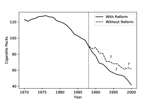
Figure 1: An example research setting for the synthetic control method (SCM): the impact of California’s 1988 tobacco control reform, Proposition 99. The goal is to construct a synthetic counterfactual trajectory to estimate what would have happened if the reform had never happened.

SCM is popular and easy to use, and in certain conditions its estimates are known to be asymptotically unbiased. However, the tool has some important flaws. Most notably, it struggles to quantify its own uncertainty. Though it is associated with a simple significance test, the tool cannot generate error bars or a confidence interval. Second, SCM is suspect to overfitting concerns. Data is noisy, both for the comparison units and for the target. There will inevitably, then, be some weighted averages that offer spurious though precise pre-reform fits. SCM’s frequentist nature leaves it vulnerable to distortion due to such spurious correlations.

In this paper, we propose a novel Bayesian approach for constructing synthetic controls. Our proposed method, the Bayesian Synthetic Control (BSC), borrows SCM’s motivating causal model and then treats the estimation problem as a probablistic modeling exercise. All estimate uncertainty is captured in the posterior distribution so that, unlike SCM, the method readily produces any desired credible (confidence) intervals. Point estimates are calculated by averaging over all plausible parameter values, an approach that protects most standard Bayesian methods from the threat of overfitting (Bishop,, 2006, p. 147). The causal model, which is shared by SCM, its frequentist derivatives, and BSC, supposes that all countries’ trajectories are driven by a few unobserved common trends. Statistically, this corresponds to a latent linear factor model. Unlike SCM, BSC estimates the latent factors explicitly.

We implement the proposed method for two previously studied research questions using the original datasets. First, we study the economic impact of German reunification in 1990 previously studied by Abadie et al., (2015), and exhibit that BSC outperforms SCM in a simple test of predictive accuracy. In this application we also show how BSC can assess the validity of its modeling assumptions through posterior predictive checking, something SCM and its frequentist derivatives cannot do. Then we examine the previously mentioned question of California tobacco controls of 1988 studied by Abadie et al., (2010) and Ben-Michael et al., (2018) among others. In the latter application, we cast partial doubt on prior findings of statistical significance, and demonstrate a method of endogenously selecting the number of latent factors included in the model. We estimate the models computationally using standard Markov Chain Monte Carlo (MCMC) posterior sampling.

The rest of this paper is structured as follows. Section 2 introduces the frequentist Synthetic Control Method and reviews related literature. In section 3, we introduce the full Bayesian Synthetic Control framework and specify its underlying probabilistic latent variable model. Sections 4 and 5 contain findings from the two empirical applications. Section 6 offers concluding remarks.

2 Synthetic Control Method and Related Work

2.1 The Synthetic Control Estimator

The SCM estimator was developed by Abadie and Gardeazabal, (2003) and formalized further by Abadie et al., (2010). The estimator is a simple weighted average of post-reform outcomes in the untreated comparison societies. The control weights are derived by minimizing a prediction loss on the pre-reform data. The loss is calculated as a weighted sum of squared errors in the variable of interest and a number of separately selected covariates. These covariates are arbitrarily chosen by the analyst but should relate to the variable of interest. They are included in the analysis for additional robustness and may mitigate the threat of overfitting.

Formally, borrowing notation from Abadie and Gardeazabal, (2003), consider a set of $J+1$ societies over $T$ years such that society $1$ faces the treatment effect in all years following some intermediate year $T_{0}$. Denote by $y_{it}$ the outcome in society $i$ at time $t$ and by $\bm{z}_{i}$ a vector of $R$ society-specific, time-invariant covariates. Collect values $y_{1t}$ for all $t\leq T_{0}$ and the entries of $\bm{z}_{1}$ into the vector $\bm{x}_{1}$ of length $R+T_{0}$. Similarly, collect into the $(R+T_{0})\times J$ matrix $\bm{X}_{0}$ the corresponding values for all other societies. Let $\bm{V}$ be a matrix of variable weights for squared error calculation (chosen separately, usually via cross-validation). Finally, let $\bm{w}$ be the vector of $J$ comparison society weights. Then, define the pre-intervention prediction loss as:

$$||\bm{x}_{1}-\bm{X}_{0}\bm{w}||_{\bm{V}}=\sqrt{(\bm{x}_{1}-\bm{X}_{0}\bm{w})^{\prime}\bm{V}(\bm{x}_{1}-\bm{X}_{0}\bm{w})}.$$ (1)

Then select the loss-minimizing synthetic control weights $\bm{w}^{*}$:

$$\bm{w}^{*} =\underset{\bm{w}}{\text{argmin}}||\bm{x}_{1}-\bm{X}_{0}\bm{w}||_{\bm{V}}$$ (2)

such that (3)

$$w_{j} \geq 0\ \forall j\text{ and }\sum_{j=2}^{J+1}{w_{j}}=1.$$ (4)

Finally, use the weights $\bm{w}^{*}$ to calculate the SCM estimator $\hat{y}_{1t}^{N}$ for the counterfactual target society value in year $t$: $\hat{y}_{1t}^{N}=\sum_{j=1}^{J+1}w_{j}y_{jt}$.

Abadie et al., (2010) show that this method can be motivated by a causal model. They assume that a number of unobserved inter-society trends drives change in the untreated outcome across all units. Formally, if we denote the untreated outcome of society $i$ in year $t$ by $y^{N}_{it}$, the authors suppose that

$$y^{N}_{it} =\delta_{t}+\bm{\theta}_{t}\bm{z}_{i}+\bm{\lambda}_{t}\bm{\mu}_{i}+\varepsilon_{it}.$$ (5)

Here $\delta_{t}$ indicates an annual fixed effect, $\bm{\theta}_{t}$ is a year-specific vector of coefficients, $\bm{z}_{i}$ represents society-specific observable covariates, $\bm{\lambda}_{t}$ is a year-specific vector of latent factors, $\bm{\mu}_{i}$ denotes a vector of factor loadings for society $i$, and $\varepsilon_{it}$ is an error term drawn from a distribution centered at zero. This specification corresponds to a latent linear factor model with unique factor loadings for each society. Some of the loadings are fixed to match the society’s time-invariant covariate values. Though SCM doesn’t estimate any model parameters explicitly, the authors use the model to prove that the SCM estimator is asymptotically unbiased under certain assumptions.

Abadie et al., (2010) also propose a relabeling-based signficance test for SCM. It involves constructing an SCM estimate for each of the comparison societies. Findings are considered statistically significant if the estimated effect is larger for the target society than for 95% of the others. Figure 2 illustrates this relabeling test.

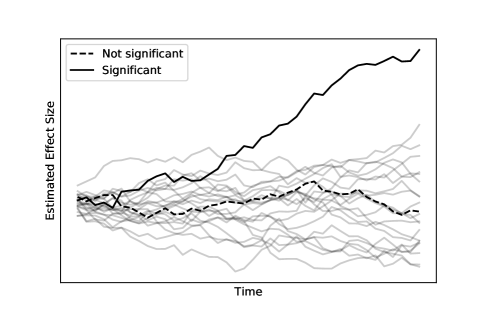
Figure 2: SCM significance test. The light lines are post-reform prediction errors for comparison societies (placebo errors). The dark ones are two alternative post-reform treatment effect estimates for the target society. The solid is considered significant, the dashed is not.

2.2 Extensions and Related Work

In addition to numerous applied studies that use SCM (eg. Aytuğ et al.,, 2017; Barlow,, 2018; Karlsson and Pichler,, 2015), recent work has further studied and extended the methodology itself. Xu, (2017) proposes the Generalized Synthetic Control (GSC), which constructs the synthetic counterfactual only after deriving an explicit point estimate for the latent factors. Ferman and Pinto, (2016) show that SCM becomes asymptotically biased if the pre-treatment match is not exact. In response, Ben-Michael et al., (2018) propose an extension to SCM, the Augmented Synthetic Control Method (ASCM), which includes a bias-reducing (though not eliminating) correction term.

Separately, Hsiao et al., (2012) develop a related panel data approach (PDA). They set up a generic latent linear factor model and show that the SCM model is its special case. Unlike SCM, PDA considers no covariate features. The authors find simulation-based evidence of worsening overfit as the number of comparison societies grows. For estimation, they use regression instead of weighted average optimization. Abadie et al., (2015) demonstrate that regression-based methods can unnecessarily rely on extrapolation when interpolation would suffice. Yet, Wan et al., (2018) show that PDA is more robust to certain assumption violations than SCM.

GSC bootstraps a confidence interval and ASCM yields a standard error, and PDA calculates a t-statistic based on estimated predictor variance. All are asymptotically valid, but none of the authors derive their predictor’s full distribution. The asymptotic behavior may thus fail if the pre-treatment period is not very long. Further, GSC and ASCM base their confidence intervals on the errors generated for comparison societies when relabeling. This prematurely uses up information that could otherwise have been used to check the method’s applicability to a particular dataset. (This task is made important by the strong assumption that a linear factor model suffices to describe the data generating process.) An obvious way to do the check is to see whether the comparison society outcomes generally fall within their predicted confidence intervals while relabeling. This cannot be done for GSC or ASCM, because comparison society confidence intervals are by design inflated to be wide enough to include the observation. Further, none of GSC, ASCM, or PDA proposes an approach to eliminate the threat of overfitting.

Finally, a research team at Google has made an early Bayesian contribution that relates to the synthetic control literature (Brodersen et al.,, 2015). In their paper, the authors describe a very general Bayesian state-space model for cross-sectional time-series variables. Inspired by synthetic controls, the authors include a regression on comparison units. The tool doesn’t have the flaws of the frequentist SCM derivatives (lack of confidence intervals, overfit, inability to check model applicability). Their approach is designed for advertising research, however, and lacks a causal model applicable to study of policy reforms.

3 The Bayesian Synthetic Control

3.1 Causal Model

Consider a set of $T$ years and $J$ societies and some quantitatively measured outcome of interest. Suppose that the outcome in certain years and societies was impacted by the unknown treatment effect of some policy intervention. Denote by $y_{it}^{T}$ and $y_{it}^{N}$ the outcome in society $i$ and year $t$ in the presence and absence of the treatment, respectively, and by $y_{it}$ the actual observed outcome. Suppose that change over time in the untreated outcome is driven by some $L$ latent inter-society trends (where $L<J$) in a linear fashion. We can then write that

$$y_{it}^{N} =\delta_{t}+\kappa_{i}+\bm{f}_{t}^{\prime}\bm{\beta}_{i}+\varepsilon_{it},$$ (6)

$$y_{it} =y_{it}^{N}+\alpha_{it}d_{it}.$$ (7)

Here $\delta_{t}$ and $\kappa_{i}$ are year and society fixed effects; $\bm{f}_{t}$ captures the factor values for the year $t$; $\bm{\beta}_{i}$ is the vector of time-invariant factor loadings of society $i$; $\varepsilon_{it}$ is random noise; $\alpha_{it}$ denotes the treatment effect in year $t$ and society $i$; and $d_{it}$ is an indicator for whether society $t$ was treated in year $i$.

BSC’s model is thus a special case of that of Hsiao et al., (2012): one of its factors is here forced to have constant unit loadings to create the year fixed effect. This is done for consistency with the SCM model of Abadie et al., (2010). The BSC model differs from the latter on two points only. BSC forces one factor to be constant over time to create a society fixed effect. More notionally, BSC also withholds from identifying a subset of the factor loadings with observed society-specific covariates.

We can stack the individual parameters together into higher-dimensional vectors and matrices: let $\bm{B}$ denote the $J\times M$ transformation matrix of factor loadings; let $\bm{F}$ denote the $T\times M$ matrix of factor values over time; let $\bm{\Delta}$ and $\bm{K}$ denote the $T\times J$ year and society fixed effect matrices, respectively; let $\bm{\varepsilon}$ denote the $T\times J$ matrix of random noise; let $\bm{A}$ and $\bm{D}$ denote the $T\times J$ treatment effect and indicator matrices, respectively; and let $\bm{Y}$ denote the $T\times J$ dimensional outcome matrix. Use $\circ$ for the elementwise (Hadamard) matrix product. Then we can describe the whole system thus:

$$\bm{Y}^{N}=\bm{\Delta}+\bm{K}+\bm{F}\bm{B}^{\prime}+\bm{\varepsilon},$$ (8)

$$\bm{Y}=\bm{Y}^{N}+\bm{A}\circ\bm{D}.$$ (9)

3.2 Estimation Goal

We observe directly $\bm{Y}$ and assert $\bm{D}$ as a known model parameter. Typically, a single society faces the treatment effect for all years following some known start year $T_{0}$. We want to investigate the untreated (reform-free) counterfactual, i.e. the posterior predictive distribution $p(\bm{Y}^{N}|\bm{Y})$. If we denote by $\bm{\theta}$ the collection of all model parameters (and assume the noise term independent from them), we can also express this as $\int p(\bm{Y}^{N}|\bm{\theta})p(\bm{\theta}|\bm{Y})d\bm{\theta}$ or, up to a normalizing constant, as $\int p(\bm{Y}^{N}|\bm{\theta})p(\bm{Y}|\bm{\theta})p(\bm{\theta})d\bm{\theta}$.

As soon as we set prior distributions for the parameters, the above integral is well defined. It is necessarily too complex for exact solving, though, so in practice it must be approximated computationally. The empirical sections of this paper do so using Markov Chain Monte Carlo (MCMC). MCMC approximates a distribution by sending a sampler on a random walk on the parameter space. Though widely used and reliable, MCMC struggles with multimodal distributions. This flaw has an important implication on one of the priors set in Section 3.3.

3.3 Distributional Assumptions

The prior distribution structure is a defining component of BSC. It is visualized using directed graph notation in Figure 3 and recorded in detail in the Supplementary Material. All random noise is assumed to follow a normal distribution with unknown constant variance. Gaussian priors are used for most other parameters, with the notable exception of the noise standard deviation and hyperparameter standard deviations. For them, the half-Cauchy distribution is used instead; Polson and Scott, (2012) argue that half-Cauchy’s fat tail makes it the most appropriate prior for scaling parameters.

Figure 3: The BSC probabilistic model as a directed graph. Nodes and arrows represent model variables and their conditional dependencies. For non-deterministic variables, vector/matrix dimension is included and the prior distribution (Normal/half-Cauchy, conditional on previous variables) visualized. All Gaussians have elementwise variances instead of covariance matrices. Outer and Hadamard products are denoted by $\otimes$ and $\circ$. Boldface denotes non-scalar; capital case denotes a matrix; $\bf{1}_{[A]}/\bf{1}_{[A\times B]}$ is a vector/matrix of ones. The full model definition is included in the Supplementary Materials.

For the society fixed effects $\kappa_{i}$ and factor loadings $\beta_{im}$, the prior is hierarchical. This means that a single Gaussian prior is used for all societies’ values, but such that its mean and variance are estimated endogenously within the model. Hierarchy biases the model against outlier values. Importantly, this prior disfavors setting anomalous factor loadings for the target society. This amounts to a soft constraint against extrapolation, a form of prediction which the developers of SCM (Abadie and Gardeazabal,, 2003; Abadie et al.,, 2010) fear less reliable than interpolation.

Most priors should be uninformative or reflect outside information. However, if the $L$ latent factors are left with identical uninformative priors, they become rotationally nonidentifiable. The nonidentifiability artifically gives the posterior distribution $L!$ identical modes, a feature that massively slows down computation for MCMC sampling. The implementations in this paper therefore match each factor with a unique, strongly informative prior. Each is a Gaussian centered around a different Principal Component Analysis (PCA) base vector. The choice of shapes was made because PCA is known to be the maximum-likelihood estimate of the latent linear factor model (Bishop,, 2006, p. 147). The PCA components are derived, before MCMC sampling, from the non-treated societies’ data. This informative prior solution has substantial flaws (mostly, it prevents the model from exploring other plausible factor modes) but is necessary barring a change from conventional MCMC sampling to another estimation strategy.

Finally, it is crucial that the treatment effect terms have near-uniform priors. Otherwise the treated data would contaminate the target society’s factor loading estimates. That would contradict the core synthetic control idea of deriving a pattern from pre-reform data and applying it post-reform.

4 Application: German Reunification

4.1 Background

One of the important papers on the original SCM methodology investigates the impact of the German reunification in 1990 (Abadie et al.,, 2015). They study the effect on per capita incomes in former West Germany. The reunification amounted to the West merging with a poorer country, so the impact ought to have been negative. Indeed, the authors find that by 2003, West German per capita GDP would have been 12% higher without the reform. We implement the BSC framework to examine this same research question.

4.2 Data

We base our work on the dataset used by the original authors which is released to the public domain (Hainmueller,, 2014). The target variable is per capita GDP adjusted for purchasing power parity (PPP). The data is originally acquired from the OECD National Accounts and Germany’s Federal Statistical Office. The dataset also includes five other covariates useful for SCM, though they play no part in the BSC implementation. The data covers West Germany and 16 OECD countries: all 23 member states from 1990, barring seven which the authors excluded due to anomalous economic development. For consistency with the prior work, we use the same set of 17 countries. The study covers years 1960-2003, of which 1990-2003 are considered treated for West Germany.

We make one alteration to the dataset. The original authors measure GDP in current US dollars rather than ones adjusted for inflation. Consequently, the variable grows at an arftifically high exponential rate. This interacts poorly with the BSC assumption that the random noise term’s variance is constant over time. One would expect the magnitude of the random error to be more or less proportional to the outcome scale. To moderate this issue, we adjust the GDP per capita figures approximately for inflation and express them in constant 2003 US Dollars. To do so, we use the US GDP deflator time series recorded from The World Bank’s World Development Indicators (The World Bank,, 2019). We rerun the replication code of Abadie et al., (2015) on the inflation-adjusted dataset, and base all BSC-SCM comparisons on the resulting SCM findings. They remain unchanged up to the precision of previously published figures.

4.3 Parameter Specification

The most notable parameter specification questions relate to the latent factors. For simplicity and ease of computation, this application presumes their number to be small at $L=4$. The first four PCA components are able to explain 0.997 of all variance in data, so the number appears sufficient. The prior for each factor is given a standard deviation greater by a factor of two than the standard deviation of the associated PCA component. (An attempt to use a factor of three failed to ensure factor identification in the posterior distribution.) The full prior distribution specification for all parameters can be found in the Supplementary Materials.

4.4 Findings

Figure 4 summarizes the empirical findings: it visualizes the resulting BSC counterfactual estimate (posterior predictive distribution) of the West German per capita GDP. The findings are largely in line with those of Abadie et al., (2015). We find that the counterfactual growth trajectory doesn’t much differ from the observed data in the first four years post-reform. Starting in 1994, however, the two trajectories diverge. By 2003, the observed GDP level is some USD 4,630, or 16.0%, below the mean predicted counterfactual value. This is equivalent to a fall in the average annual growth rate by 1.1 percentage points, from over 1.9% to just under 0.9%. SCM predicts a similar though slightly smaller gap: USD 3,360, or 11.7%, which corresponds to a 0.7 fall in the average growth rate.

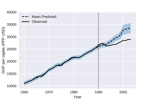
Figure 4: The BSC posterior predictive distribution of the counterfactual West German per capita GDP (2003 PPP USD) without reunification. The dashed trajectory and the shaded region represent the distribution’s mean and 95%-confidence interval (CI). The CI includes error re-sampling for the full time period. Observed data is represented by the solid line.

Importantly, from 1994 onwards, the observed data falls far outside the credible interval (CI) of the posterior predictive distribution. By 2003, the 95%-CI of the treatment effect is USD 2,570 - 6,680. Figure 5 illustrates this in more detail. On the left it depicts the treatment effect’s mean and 95%-CI by year; the right panel draws the full posterior distribution for the effect by the end year 2003. The figure illustrates how the treatment effect grew significant around 1994. It also shows how BSC gives a near-zero probability for an overall nonnegative treatment effect. The West German per capita income almost certainly fell due to reunification.

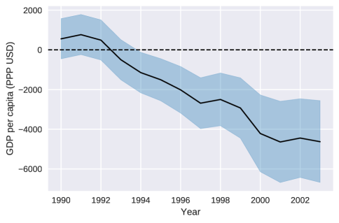
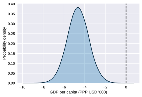
Figure 5: BSC posterior distribution of the reunification’s treatment effect on West German per capita GDP (2003 PPP USD). Left panel plots the mean and 95%-CI of the effect by year. Right panel visualizes the full distribution of the treatment effect at the year 2003, i.e. the aggregate effect over the full post-reform time period.

As a plausibly interesting side effect, BSC also generates full probabilistic estimates of all other model parameters. (In this it differs substantially from its frequntist counterparts.) An example is provided in Figure 6 which graphs each of the latent factor posterior distributions. Closer analysis could identify correspondence between these factors and observed international trends, such as global overall productivity growth (Component 1) or energy prices (possibly Component 3). Using the factor loading estimates, for their part, we could measure similarity between countries and group them into clusters.

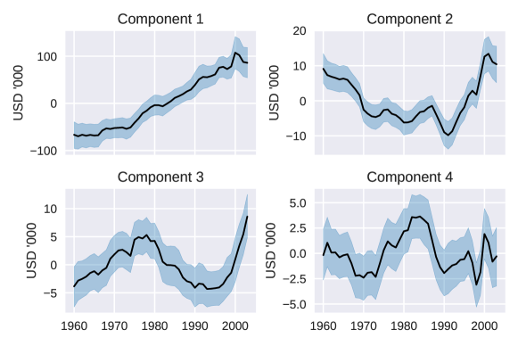
Figure 6: BSC posterior distribution of each of the latent factors. The solid trajectory and the shaded region represent the mean and the 95%-CI of the distribution. The factors are numbered in the order of descending variance of the PCA component around wich the prior of the factor is centered.

BSC’s ability to yield findings on the other parameters could in this fashion prove useful for political scientific attempts to bridge the gap between quantitative findings and qualitative interpretation or explanation, i.e. to ”put qualitative flesh on quantitative bones” (Tarrow,, 1995). Abadie et al., (2015) think this one of the major goals of the synthetic control approach. It must be noted, though, that these secondary parameter estimates do not contain any additional information on the size of the treatment effect.

4.5 Prediction Accuracy Comparison to SCM

A relabeling exercise provides an excellent opportunity for accuracy comparison between BSC and SCM. To do so, we use each framework to predict in turn the observed post-treatment trajectory of each of the comparison societies. At each run, we measure the distance between the prediction and the observation. The more accurate the method, the shorter the distance ought to be. To do so with BSC, we use the posterior predictive mean as our point estimate. We visualize the comparison society average of the error for each year and framework in Figure 7. Overall, the findings show that BSC exhibits greater predictive accuracy on this dataset. In most years, it is on average over two percentage points closer to reality than SCM. A likely explanation for the improvement in accuracy is BSC’s freedom of overfit concerns. Evidence on further datasets and simulations is required for a more reliable comparison.

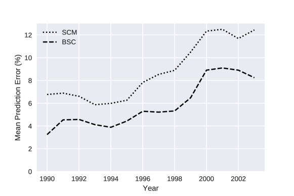
Figure 7: Accuracy comparison of BSC and SCM. The dotted line maps the average absolute error of SCM when the method is used to predict the comparison societies’ outcomes in each year. The dashed line does so for BSC. Error is measured as percentage of the observed outcome value.

4.6 Model Validity Checking

A linear factor model makes strong assumptions about the data-generating process, assumptions which are bound to be more or less violated in reality. The severity of those violations, and the severity of their consequences on predictive accuracy, is a question of crucial interest in any real-world application. Prior literature suggests that posterior predictive checking may be the most useful way to study the scale and nature of such issues (Gelman and Shalizi,, 2013). It refers to testing whether the model predictions are compatible with observed data.

The relabeling exercise provides an obvious way for running posterior predictive checks on BSC. When the model is used to predict a comparison society post-reform trajectory, the posterior predictive distribution should include the observed data in its spread. Figure 8 exhibits the results of this test. The dotted and dashed lines indicate, for each year, the share of comparison societies for which the observed trajectory falls outside the 95% and 99%-CI, respectively. The solid graph reflects the share of total prediction failures. This refers to cases where the observed data is more extreme than any single draw from the estimated posterior predictive distribution, i.e. it receives the p-value of zero.

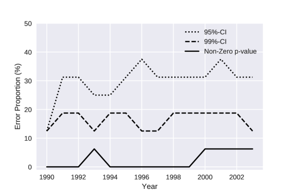
Figure 8: BSC test of model validity on the German reunification data. The graph visualizes findings from a relabeling exercise where BSC was used to predict the comparison societies’ outcomes. The dotted and dashed lines indicate the proportion of outcomes that fell outside their predicted 95%-CI and 99%-CI, respectively. The solid line indicates the proportion of outcomes that were estimated to have a posterior probability density of zero.

The share of predictions that lie within the 95%-CI starts close to 90% in 1990, but soon falls to around two thirds and stabilizes at that level. The wider 99%-CI performs better, consistently capturing the observed data 80-90% of the time. Complete prediction failures are very infrequent, with only a handful of years seeing even one single occurrence. Perhaps surprisingly, none of the graphs demonstrates a clear upward trend over time. The findings clearly demonstrate, first, that the modeling assumptions are indeed violated. Second, the importance of those violations is notable and fairly constant over the studied 14-year timespan.

At the same time, the results are not altogether hopeless. The confidence intervals include observed data most of the time, even if less often than they should. The 95%-CI succeeds more than two thirds of the time and the wider intervals perform better still. This suggests that the linear factor model, when accompanied by BSC’s probabilistic structure, is a useful even if imprecise model for GDP per capita growth in the OECD 1960-2003.

Note that this consistency check cannot be carried out for SCM, GSC, ASCM, or any other method that uses up the relabeling findings to calculate significance or confidence intervals. They artificially inflate their confidence bounds to include the comparison society observed data most of the time. This may hide warning signs of assumption violations, which is dangerous because both the point estimates and the confidence intervals are valid only to the extent that the assumptions hold up. Lack of validity checking makes analysis prone to overtly confident research conclusions.

5 Application: California Tobacco Control Program

5.1 Background

The second canonical SCM paper examines the effect of a 1988 tobacco control reform on California’s cigarette consumption (Abadie et al.,, 2010). The reform, known as Proposition 99, introduced sin tax hikes and other anti-smoking measures. The authors find that the reform’s effect amounted to a 25% fall in cigarette sales. The study is famous for introducing the relabeling based significance test for SCM. Ben-Michael et al., (2018) note the frequency at which the question has been re-analyzed. We join in on this effort and study the same research question using BSC.

5.2 Data

The original authors’ outcome variable is the number of cigarette packs sold per capita (as per tax data). As comparison societies they use a set of 38 other US states, or all states that didn’t introduce major tobacco controls of their own. The time period covered is 1970-2000, of which the years 1989-2000 form a treatment period for California. For consistency, we use the same selection of data and acquire it from a more recent edition of the publication used by the original authors (Orzechowski and Walker,, 2014). We ignore the other covariates included in the SCM analysis.

5.3 Selecting the Number of Latent Factors

Section 4 fixed the number of latent factors at $L=4$. That choice of $L$ was computationally useful, especially when running the heavy relabeling exercise, but arbitrary from a modeling point of view. In this application we propose a way of choosing $L$ through formal model selection. Namely, the model can be run repeatedly with different values of $L$, recording a measure of predictive performance at each round. The choice of measure is not obvious, but one robust option is the Watanabe-Akaike Information Criterion (WAIC). WAIC is known to be asymptotically equivalent to measuring the model’s predictive accuracy with repeated cross-validation (Watanabe,, 2010).

The choice of $L$ in this section begins with the a priori assertion that $L\in\{3,4,5,6,7,8\}$. The set is limited to be fairly small because large values are computationally expensive. Further, the variance of each latent factor’s PCA-centered prior is proportional to that of the PCA component, so ever smaller for every additional included factor. This urges caution against increasing the number of factors endlessly even in the face of improving predictive accuracy, so as not to introduce parameters with arbitrarily strongly informative priors.

The resulting WAIC values are collected in Table 1. The value is decreasing in the number of included factors. Smaller WAIC indicates better predictive performance, so we choose the model with the most factors: $L=8$. The full prior specification for all other parameters is again included in the Supplementary Materials.

$L$	3	4	5	6	7	8
WAIC	7308	6834	6616	6538	6450	6326

Table 1: Model comparison findings for the number of latent factors. The table records the Watanabe-Akaike Information Criterion (WAIC), an asymptotic Bayesian model comparison statistic, for six alternative BSC model specifications on the California dataset. The specifications differ by the number of latent factors. A smaller value indicates superior predictive performance.

5.4 Findings

The core findings are captured in Figure 9 which plots the mean predicted counterfactual trajectory and its 95%-CI along with the observed data. Like previous work, the BSC model finds that the counterfactual trajectory falls slower than the observed smoking rate. The two trajectories don’t diverge notably for the first couple of years after the reform. Starting around 1992, however, the gap begins to grow more substantial. By 2000, the predicted rate is 64.0 packs per person, or almost 22.4 packs (54%), greater than the observed rate.

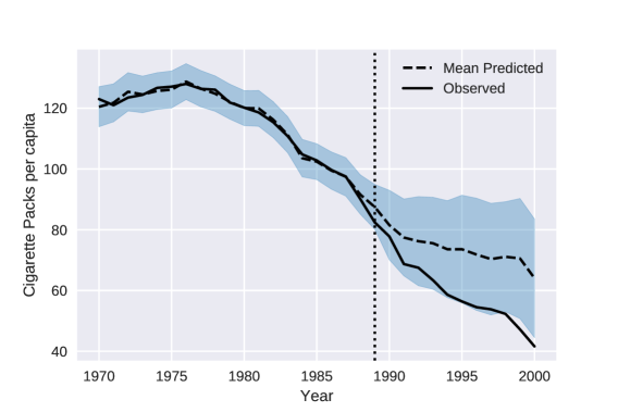
Figure 9: The BSC posterior predictive distribution of the counterfactual cigarette consumption trajectory without the passing of Proposition 99. The dashed trajectory and the shaded region represent the distribution’s mean and 95%-confidence interval (CI). The CI includes error re-sampling for the full time period. Observed data is represented by the solid line.

The BSC findings are quite similar to those of Abadie et al., (2015) when it comes to the scale of the treatment effect. We find that the the reform reduced smoking over the 1989-2000 period by 15.4 annual packs per person, or by 23%. The reported SCM estimate is slightly larger at approximately 25%. For further comparison, Ben-Michael et al., (2018) report some predicted counterfactual effects for the particular year 1997. The predictions are 26 per capita for SCM and 20 or 13 for two different Augmented SCM (ASCM) implementations. The BSC mean estimate for 1997 is 16.5 packs, so it falls well into the spread of the frequentist point estimates.

However, BSC’s ability to quantify its uncertainty reveals that the treatment effect’s significance is dubious. Note how the observed trajectory remains within the shaded 95%-CI throughout most of the post-reform time period. Up to 1997, the model yields a probability of over 5% that, even without the reform, tobacco consumption would have been as far from the prediction mean as the observed trajectory. The treatment effect becomes significant in 1998-2000, but just barely so. The full posterior distribution of the effect is illustrated in Figure 10.

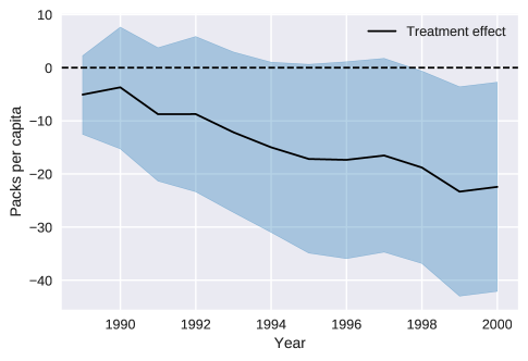
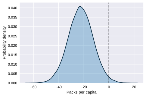
Figure 10: BSC posterior distribution of Proposition 99’s treatment effect on cigarette consumption in California. Left panel plots the mean and 95%-CI of the effect by year. Right panel visualizes the full distribution of the treatment effect at year 2000, i. e. the aggregate effect over the full post-reform time period.

These significance findings differ somewhat from those of previous studies. Abadie et al., (2015) find stronger evidence, with the treatment effect becoming significant as early as 1993. Ben-Michael et al., (2018), instead, conclude that the effect was insignificant throughout. They exhibit a frequentist two-standard error interval for each of their three tested frequentist SCM/ASCM specifications, and show that a nonnegative effect falls well within each interval. (It should be noted that the frequentist synthetic controls’ sampling distributions are unknown, so the two-standard error bound isn’t guaranteed to correspond to a 95%-CI.)

In conclusion, BSC’s point estimates in the California tobacco control case resemble those of previous researchers. On statistical significance, however, BSC disagrees with its frequentist counterparts. Unlike SCM, it finds the treatment effect insignificant (in the Bayesian sense) for most of the post-reform time period. Yet unlike ASCM, it deems the effect significant by the end year 2000, even if just barely so. This disagreement between the various methods emphasizes the importance of the choice of method for constructing synthetic controls. In the face of such disagreement BSC is a very appealing choice, especially because its credible intervals are valid on finite samples rather than asymptotically.

6 Conclusion

This paper’s main contribution is the design for the Bayesian Synthetic Control (BSC), a novel statistical framework for the counterfactual estimation problem thus far mostly addressed using the synthetic control method (SCM). Like SCM and its frequentist extensions, BSC is based on a linear factor model. It has certain strengths over those preceding methods: (1) it describes in full the associated prediction uncertainty, including valid finite sample credible intervals; (2) its Bayesian nature protects it from overfitting; and (3) it enables the use of relabeling to check model validity.

We implement BSC on two previously studied research questions, the German reunification and a California tobacco control program. In the former case BSC yields similar findings as SCM but outperforms it in a simple test of predictive accuracy. This may be due to an overfitting issue in SCM. This empirical section also illustrates BSC’s unique ability to use relabeling to assess model validity. In the California case, BSC casts doubt on prior researchers’ (mutually contradictory) findings on statistical significance. Together, the applications show that BSC is ready for implementation in practical research settings.

The proposed framework continues to have notable limitations. Importantly, unnecessarily restrictive PCA-based priors are used for latent factor trajectories. This is done to aid computation in the Markov Chain Monte Carlo (MCMC) implementation. Future research could examine whether a change of estimation strategy (e.g. to variational inference or stochastic gradient MCMC) would eliminate the need for this restriction. Similarly, the proposed approach to the number of latent factors is not ideal: Bayesian model averaging would likely be preferable to model selection using WAIC. Both limitations are related to a third flaw, characteristic of many modern Bayesian methods: BSC is computationally much heavier than its frequentist counterparts.

Due to its Bayesian estimation goal, that of describing the posterior (predictive) distribution, BSC doesn’t depend on the asymptotic qualities of any particular estimator. Thus, its modeling assumptions can be seamlessly altered. It is trivially easy to include two or more treated societies. Missing data points in comparison societies could be addressed with similar ease by marking them as stand-alone treated years, a feature that markedly relaxes data availability restrictions. Other extensions, like nonlinear factors, nonconstant noise term variance, and lagged outcomes or other time series behavior, could also be included without rethinking the implementation strategy.

To our knowlegde, the present paper represents the first explicit attempt to solve the synthetic control counterfactual estimation problem for policy reforms in the Bayesian paradigm. The model, though still subject to certain flaws, is demonstrably ready for real world applications and competitive in performance to existing frequentist tools. This paper may then hopefully spur further research into Bayesian solutions to the synthetic control problem and other related topics in causal inference.

References

- Abadie et al., (2010) Abadie, A., Diamond, A., and Hainmueller, J. (2010). Synthetic control methods for comparative case studies: Estimating the effect of California’s tobacco control program. Journal of the American Statistical Association, 105(490):493–505.
- Abadie et al., (2015) Abadie, A., Diamond, A., and Hainmueller, J. (2015). Comparative politics and the synthetic control method. American Journal of Political Science, 59(2):495–510.
- Abadie and Gardeazabal, (2003) Abadie, A. and Gardeazabal, J. (2003). The economic costs of conflict: A case study of the Basque country. American Economic Review, 93(1):113–132.
- Aytuğ et al., (2017) Aytuğ, H., Kütük, M. M., Oduncu, A., and Togan, S. (2017). Twenty years of the EU-Turkey customs union: A synthetic control method analysis. Journal of Common Market Studies, 55(3):419–431.
- Barlow, (2018) Barlow, P. (2018). Does trade liberalization reduce child mortality in low- and middle-income countries? A synthetic control analysis of 36 policy experiments, 1963-2005. Social Science & Medicine, 205:107–115.
- Ben-Michael et al., (2018) Ben-Michael, E., Feller, A., and Rothstein, J. (2018). The augmented synthetic control method. Arxiv open access.
- Bishop, (2006) Bishop, C. (2006). Pattern Recognition and Machine Learning. Springer Science.
- Brodersen et al., (2015) Brodersen, K., Gallusser, F., Koehler, J., Remy, N., and Scott, S. (2015). Inferring causal impact using Bayesian structural time-series models. Annals Of Applied Statistics, 9(1):247–274.
- Ferman and Pinto, (2016) Ferman, B. and Pinto, C. (2016). Revisiting the synthetic control estimator. Open access.
- Gelman and Shalizi, (2013) Gelman, A. and Shalizi, C. R. (2013). Philosophy and the practice of Bayesian statistics. British Journal of Mathematical and Statistical Psychology, 66(1):8–38.
- Hainmueller, (2014) Hainmueller, J. (2014). Replication data for: Comparative politics and the synthetic control method. Harvard Dataverse.
- Hsiao et al., (2012) Hsiao, C., Ching, S., and Wan, S. K. (2012). A panel data approach for program evaluation: Measuring the benefits of political and economic integration of Hong Kong and mainland China. Journal of Applied Econometrics, 27(5):705–740.
- Karlsson and Pichler, (2015) Karlsson, M. and Pichler, S. (2015). Demographic consequences of HIV. Journal of Population Economics, 28(4):1097–1135.
- Orzechowski and Walker, (2014) Orzechowski and Walker (2014). The Tax Burden on Tobacco. Historical Compilation, 49 edition.
- Polson and Scott, (2012) Polson, N. G. and Scott, J. G. (2012). On the half-Cauchy prior for a global scale parameter. Bayesian Analysis, 7(4):887–902.
- Tarrow, (1995) Tarrow, S. (1995). Bridging the quantitative-qualitative divide in political science. American Political Science Review, 89(2):471–474.
- The World Bank, (2019) The World Bank (2019). World Development Indicators.
- Wan et al., (2018) Wan, S.-K., Xie, Y., and Hsiao, C. (2018). Panel data approach vs synthetic control method. Economics Letters, 164:121–123.
- Watanabe, (2010) Watanabe, S. (2010). Asymptotic equivalence of Bayes cross validation and Widely Applicable Information Criterion in singular learning theory. Journal Of Machine Learning Research, 11:3571–3594.
- Xu, (2017) Xu, Y. (2017). Generalized synthetic control method: Causal inference with interactive fixed effects models. Political Analysis, 25(1):57–76.