BeyondBenford: An R Package to Determine Which of Benford’s or BDS’s Distributions is the Most Relevant

Abstract

The package BeyondBenford compares the goodness of fit of Benford’s and Blondeau Da Silva’s (BDS’s) digit distributions in a dataset. The package is used to check whether the data distribution is consistent with theoretical distributions highlighted by Blondeau Da Silva or not: this ideal theoretical distribution must be at least approximately followed by the data for the use of BDS’s model to be well-founded. It also allows to draw histograms of digit distributions, both observed in the dataset and given by the two theoretical approaches. Finally, it proposes to quantify the goodness of fit via Pearson’s chi-squared test.

1 Introduction

Benford’s Law, also called Newcomb-Benford’s Law, is somewhat surprising; indeed, the first digit $d$, $d\in\llbracket 1,9\rrbracket$, of numbers in many naturally occurring collections of data does not follow a discrete uniform distribution, as might be thought, but a logarithmic distribution (see the recent books of [Mil15] and [BH15]). Discovered by the astronomer Newcomb in $1881$ [New81], it was definitively brought to light by the physicist Benford in $1938$ [Ben38]. The probability that $d$ is the first digit of a number is approximately:

$$\log(1+\frac{1}{d})\enspace.$$

It can also be extended to digits beyond the first one [Hil95], the probability for $d$, $d\in\llbracket 0,9\rrbracket$, to be the $p^{\text{th}}$ digit of a number being:

$$\sum_{j=10^{p-2}}^{10^{p-1}-1}\log(1+\frac{1}{10j+d})\enspace.$$

It was quickly admitted that numerous empirical data sets follow Benford’s law: economic data [SHK05], social data [Gol15], demographic data [NW95, LSE00], physical data [Knu69, BK91, NM07, AL14] or biological data [CLRTFM08, FGPM12] for instance; to such an extent that this law was used to detect possible frauds in lists of socio-economic data [Var72, Nig99, DHP04, Sav06, Tö09, RGBE11] or in scientific publications [AYS14].

Nevertheless many discordant voices brought a significantly different message. By putting aside the distributions known to fully disobey Benford’s law [Rai76, Hil88, TBL00, SF01, Bee09, DMO11], this law often appeared to be a good approximation of the reality, but no more than an approximation [SF01, Sav06, DMO11, GD11, Goo16].

Similar to first digit case, the distributions of digits beyond the first have been observed in various application areas [Gey10, AL14, AYS14] and have also been used to detect frauds [Car88, Tho89, MJ06, CG07, Die07, Joe13]. Once more, limits of such methods were emphasized [MJ06, CG07, Die07].

Blondeau Da Silva, considering data as realizations of a homogeneous and expanded range of random variables following discrete uniform distributions, showed that, the proportion of each $d$, $d\in\llbracket 0,9\rrbracket$, as leading digit [BDS19] or as other digit [BDS18] structurally fluctuates. He demonstrated that, in his models, the predominance of $1$ as digit (followed by $2$ and so on) is all but surprising, and that the observed fluctuations around the values of probability determined by Benford’s Law are also predictible: there is not a single Benford’s Law but numerous distinct laws each of them determined by a parameter, the upper-bound of the considered data.

The huge and growing literature on Benford’s law is available on the online database www.benfordonline.net with well over $1000$ papers. Two CRAN Packages already enable to check whether datasets conform to Benford’s law or not: BenfordTests and benford.analysis. The package BeyondBenford compares the goodness of fit of Benford’s Law, on the one hand, and BDS’s Laws, on the other hand. Indeed, these latter, under certain conditions that we will recall, allow a better reliability of adjustment. The package BeyondBenford calculates the digit distribution in the considered dataset and determines whether it is consistent with BDS’s or Benford’s one. It also provides plotting tools for the visual evaluation of these distributions. We will walk through a detailed example to give an overview of the BeyondBenford package.

2 An example to get familiar with the main functions

Street addresses of Pierre-Buffiere, a small town of approximately $1200$ inhabitants in Haute-Vienne (France), are available on:

www.data.gouv.fr/fr/datasets/base-d-adresses-nationale-ouverte-bano/ ,

which is an open platform for French public data.

After loading the package (library(BeyondBenford)), the code data(address_PierreBuffiere) gives us access to the sample data. This factor contains $346$ rows, with each row representing an address number.

3 Are the data consistent with BDS’s model?

This is the first essential question that must be answered in the affirmative. If this is not the case, comparisons are not relevant: the package should not be used. Indeed the use of the package is appropriate when the studied data can be considered as realizations of a homogeneous and expanded range of random variables approximately following discrete uniform distributions. In this model, the data is strictly positive and is upper-bounded, constraint which is often valid in datasets, the physical, biological, demographic, social and economical quantities being limited [BDS19].

Among the different domains studied by Benford [Ben38], some could be well adapted to our model: sizes of populations or street addresses for example (see [BDS19] for a detailed explanation). [JDLR04] advised precisely to use their own similar model in the case of street addresses or when considering the first-page numbers of articles in a bibliography.

[BDS18] showed that the model induces a specific distribution of positive integers determined by an upper-bound. Hence, in order to conform as closely as possible to the model, the studied database must have a distribution similar to that described in [BDS18]. In $p^{\text{th}}$ digit case, the probability $p_{k}$ to obtain the number $k\in\llbracket 10^{p-1};u_{b}\rrbracket$ (where $u_{b}$ is the upper-bound) verifies:

$$p_{k}=\frac{1}{u_{b}-10^{p-1}+1}\sum_{i=k+1-10^{p-1}}^{u_{b}+1-10^{p-1}}\frac{1}{i}\enspace.$$

In the studied example, the maximum value of the street number is $74$. The associated theoretical distribution for the second digit is plotted in Figure 1.

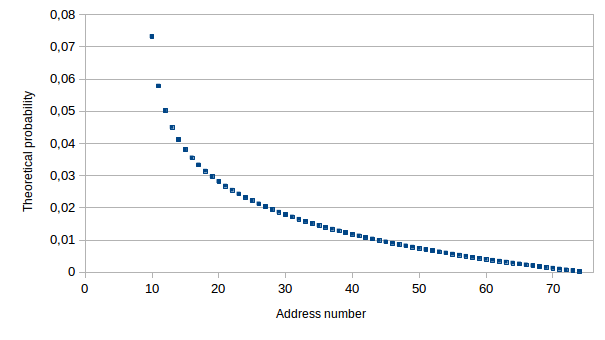
Figure 1: Theoretical distribution of street numbers in the second digit case, the upper-bound being $74$.

The BeyondBenford package provides plotting tools to determine whether the data is consistent with BDS’s model: the function dat.distr. The function’s arguments are as follows:

1. dat: the considered dataset, a data frame containing non-zero real numbers.

2. xlab: the $x$-axis label. Default value: xlab="data".

3. ylab: the $y$-axis label. Default value: xlab="Frequency".

4. main: the title of the graph. Default value: main="Distribution of data".

5. theor: if theor=TRUE BDS’s theoretical distribution is plotted, otherwise only the histogram is represented. Default value: theor=TRUE.

6. nclass: a strictly positive integer: the number of classes in the histogram. Default value: nclass=50.

7. col: the color used to fill the bars of the histogram. NULL yields unfilled bars. Default value: col="lightblue".

8. conv: if conv=1, all values of the dataset are multiplied by $10^{k}$ where $k$ is the smallest positive integer such that all non-zero numerical values in the newly multiplied data frame have an absolute value greater than or equal to $1$. Default value: conv=0.

9. upbound: a positive integer, which characterizes the data. All (or most) of the data are lower than this "upper-bound". Default value: upbound=ceiling(max(dat)).

10. dig: the chosen position of the digit (from the left). Default value: dig=1.

11. colt: the color used to plot BDS’s theoretical distribution. Default value: colt="red".

12. ylim: a two-components vector: the range of $y$ values. Default value: ylim=NULL.

13. border: the color of the border around the bars. Default value: border="blue".

14. nchi: the number of classes for values from $10^{p-1}$ to max(max(data),upbound). If nchi>0, the function returns the chi-squared statistic (with $nchi-1$ degrees of freedom) of goodness of fit determined by the different classes. The null hypothesis states that the studied distribution is consistent with the considered theoretical distribution. Default value: nchi=0.

15. legend: if legend=TRUE, the legend is displayed. Default value: legend=TRUE.

16. bg.leg: the background color for the legend box. Default value: bg.leg="gray85".

Let us apply the dat.distr function to the address_PierreBuffiere dataset. The output from dat.distr is the data histogram along with optional BDS’s theoretical distributions (Figure 2).

Example 1.

## Both the histogram and theoretical distribution are represented
dat.distr(address_PierreBuffiere, dig=2, nclass=65)

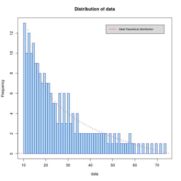
Figure 2: The data histogram of street numbers in the second digit case and its BDS’s theoretical distribution.

Note that, out of the $346$ values, only $217$ are taken into consideration here because the values need to have at least $2$ digits.

The data distribution looks similar to the one described by BDS’s model (Figure 2). Let us provide a second example in which we numerically determine whether the studied distribution is conform to the theoretical distribution or not:

Example 2.

## The function returns the chi-squared statistic of goodness of fit determined by nchi classes.
dat.distr(address_PierreBuffiere, dig=2, nchi=4)
$[$1$]$ "Class freq.:" "130" "51" "25"
$[$5$]$ "11"
$[$1$]$ "Theor. freq.:" "127.050977504473" "54.6446927640259" "26.7009825219254"
$[$5$]$ "8.60334720957567"
                    chi2                    pval
1    Chi2 value is:   The p-value is:
2 1.08754607580421 0.780081329402347

The dat.distr function returns, if requested, the frequencies of each equal-sized class of the dataset and the associated theoretical frequencies. It also returns a data frame containing the value of the chi squared test-statistic and its p-value. Note that the number of classes is limited by the theoretical frequencies that cannot exceed $5$ in Pearson’s chi-squared test [Pea00]. In our example, the null hypothesis cannot be rejected: the studied distribution is consistent with the theoretical distribution.

4 Comparisons of the goodness of fit of Benford’s and BDS’s digit distributions in a dataset

4.1 Raw data

The package BeyondBenford provides a function returning the frequencies of each figure at a given position in the considered dataset: obs.numb.dig. Its two arguments dat and dig have already been defined in dat.distr function. The function output is a vector containing the frequencies of each figure in ascending order.

Let us give an example:

Example 3.

obs.numb.dig(address_PierreBuffiere, dig=2)
$[$1$]$ 31 24 27 21 25 17 21 16 19 16

For instance, there are $25$ values with the second digit being a $4$.

The package BeyondBenford also provides a function returning Benford’s probability that a figure is at a given position: Benf.val. Its argument dig has already been defined in dat.distr function. Its second argument fig stands for the considered figure.

Let us give an example:

Example 4.

Benf.val(4, dig=2)
$[$1$]$ 0.1003082

The package BeyondBenford at last provides a function returning BDS’s probability that a figure is at a given position (once the associated upper-bound has been specified): Blon.val. Its three arguments dig, upbound and fig have already been defined above.

Let us give an example:

Example 5.

Blon.val(fig=4, dig=2,upbound=74)
$[$1$]$ 0.09836642

In Table 1 below, the frequencies of each figure in the considered dataset, regarding the second digit of address numbers, are listed.

Figure	Frequency in the database	BDS’s values	Benford’s values
$0$	$0.1429$	$0.1436$	$0.1197$
$1$	$0.1106$	$0.1247$	$0.1139$
$2$	$0.1244$	$0.1136$	$0.1088$
$3$	$0.0968$	$0.1053$	$0.1043$
$4$	$0.1152$	$0.0984$	$0.1003$
$5$	$0.0783$	$0.0924$	$0.0967$
$6$	$0.0968$	$0.0872$	$0.0934$
$7$	$0.0737$	$0.0825$	$0.0904$
$8$	$0.0876$	$0.0782$	$0.0876$
$9$	$0.0737$	$0.0742$	$0.0850$

Table 1: Values of frequency of each figure as second digit in the database, Benford’s and BDS’s theoretical values (the chosen upper-bound being $74$). These values are rounded to the nearest ten-thousandth.

The BDS’s theoretical values seem slightly better; in particular the frequency range is higher, both for the observed data and for BDS’s theoretical values.

4.2 Plotting tools

The BeyondBenford package provides plotting tools to perform the comparison between the two models with the function digit.distr. In addition to arguments that are shared with dat.distr (dat, dig, upbound, main), the digit.distr function has the following additional arguments:

1. mod: if mod="ben", the data histogram and that of Benford are displayed, if mod="ben$\&$blo", the data histogram, that of Benford and that of BDS are plotted, and otherwise the data histogram and that of BDS are given. Default value: mod="ben".

2. col: a vector containing two colors used to fill the bars of the histogram, if mod="ben". Default value: col=c("#FFFFAA", "#AAFFAA").

3. colbebl: a vector containing three colors used to fill the bars of the histogram, if mod="ben$\&$blo". Default value: colbebl=c("#FFFFAA", "#AAFFAA", "#AAFFFF").

4. colbl: a vector containing two colors used to fill the bars of the histogram, if the latter case. Default value: colbl=c("#FFFFAA", "#AAFFFF").

5. legend: if legend=TRUE, the legend is displayed. Default value: legend=TRUE.

6. leg: a two-components vector containing text appearing in the legend, if mod="ben". Default value: leg=c("Observed", "Benford").

7. legbebl: a three-components vector containing text appearing in the legend, if mod="ben$\&$blo". Default value: legbebl=c("Observed", "Benford", "Blondeau").

8. legbl: a two-components vector containing text appearing in the legend, if the latter case. Default value: legbl=c("Observed", "Blondeau").

Let us apply the digit.distr function to the address_PierreBuffiere dataset. The output from dat.distr is a histogram of theoretical and experimental digit distribution (Figure 3).

Example 6.

digit.distr(address_PierreBuffiere, dig=2, mod="ben$\&$blo")

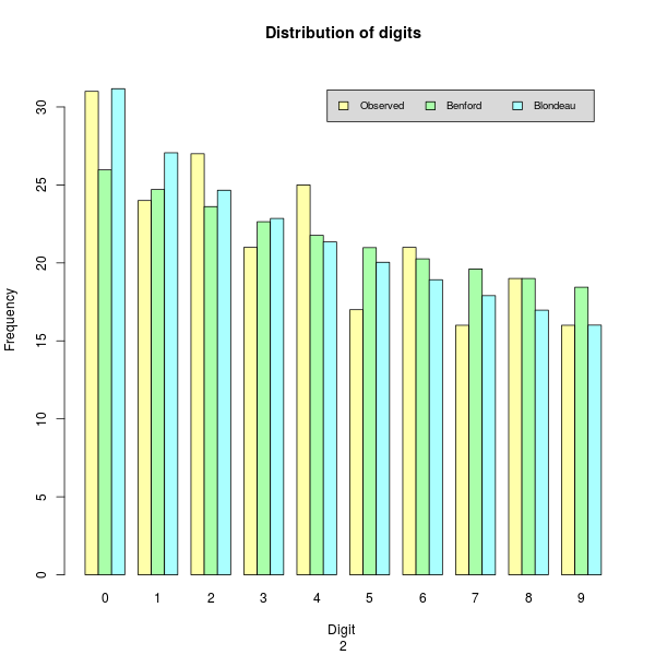
Figure 3: The histogram of Pierre Buffière’s street numbers in the second digit case along with Benford’s and BDS’s distributions of digit.

Naturally, Figure 3 is consistent with Table 1.

4.3 Pearson’s chi-squared test

To quantify the quality of theorical models, we use Pearson’s chi-squared test of goodness of fit [Pea00]: the null hypothesis states that the studied distribution is consistent with the considered theoretical distribution, i.e. Benford’s or BDS’s ones. The function chi2 determines the test statistic and its associated p-value. In addition to arguments that are shared with dat.distr (dat, dig, upbound), the chi2 function has the following specific arguments:

1. mod: if mod="ben", the theorical distribution considered is that of Benford, else it is BDS’s ones which is chosen. Default value: mod="ben".

2. pval: if pval=0, the p-value is not returned, else it is available. Default value: pval=0.

Let us apply this function to the address_PierreBuffiere dataset. The output from chi2 is a data frame containing the Pearson’s chi-squared statistic (and the associated p-value if requested).

Example 7.

## Measure of Benford’s Law goodness of fit
chi2(address_PierreBuffiere, dig=2, pval=1)
                    chi2                    pval
1    Chi2 value is:   The p-value is:
2 3.84793221030181 0.921132993758269

## Measure of BDS’s Law goodness of fit
chi2(address_PierreBuffiere, dig=2, pval=1, mod="BDS")
                    chi2                    pval
1    Chi2 value is:   The p-value is:
2 2.47996278328848 0.981417506807756

In both cases the null hypothesis cannot be rejected: the studied distribution is consistent with the theoretical distributions. It can be noted that the quality of the adjustment seems slightly better with BDS’s model.

5 Conclusion

The use of Benford’s Law has increased rapidly in the last few years in extremely diverse fields such as mathematics, physics, biology, economics and demography, to name but a few. But the adjustment proposed by Benford is often only approximate. In some precisely described cases, it is BDS’s probability distributions that are preferred. Indeed the probabilies of occurrence of digits in these distributions fluctuate around Benford’s values [BDS19, BDS18].

The BeyondBenford package is thus a relevant tool to compare the goodness of fit of Benford’s and BDS’s distributions in a given collection of data and to offer new laws to find a better approximation of digits distribution in the considered dataset.

References

- [AL14] T. Alexopoulos and S. Leontsinis. Benford’s Law in astronomy. Journal of Astrophysics and Astronomy, 35(4):639–648, 2014.
- [AYS14] A. D. Alves, H. H. Yanasse, and N. Y. Soma. Benford’s Law and articles of scientific journals: comparison of JCR and Scopus data. Scientometrics, 98:173–184, 2014.
- [BDS18] S. Blondeau Da Silva. Benford or not Benford: new results on digits beyond the first. arXiv:1805.01291 [stat.OT], 2018.
- [BDS19] S. Blondeau Da Silva. Benford or not Benford: a systematic but not always well-founded use of an elegant law in experimental fields. Communications in Mathematics and Statistics, 2019.
- [Bee09] T. W. Beer. Terminal digit preference: beware of benford’s law. Journal of Clinical Pathology, 62(2):192, 2009.
- [Ben38] F. Benford. The law of anomalous numbers. Proceedings of the American Philosophical Society, 78:127–131, 1938.
- [BH15] A. Berger and T. Hill. An Introduction to Benford’s Law. Princeton University Press, Princeton, NJ, 2015.
- [BK91] J. Burke and E. Kincanon. Benford’s law and physical constants: the distribution of initial digits. American Journal of Physics, 59:952, 1991.
- [Car88] C. Carslaw. Anomalies in income numbers: Evidence of goal oriented behavior. The Accounting Review, 63(2):321–327, 1988.
- [CG07] W. K. T. Cho and B. J. Gaines. Breaking the (Benford) Law: Statistical fraud detection in campaign finance. The American Statistician, 61(3):218–223, 2007.
- [CLRTFM08] E. Costasa, V. Lopez-Rodasa, F. Torob, and A. Flores-Moya. The number of cells in colonies of the cyanobacterium microcystis aeruginosa satisfies benford’s law. Aquatic Botany, 89(3):341–343, 2008.
- [DHP04] C. Durtschi, W. Hillison, and C. Pacini. The effective use of benford’s law to assist in detecting fraud in accounting data. Journal of Forensic Accounting, V:17–34, 2004.
- [Die07] A. Diekmann. Not the first digit! Using benford’s law to detect fraudulent scientific data. Journal of Applied Statistics, 34(3):321–329, 2007.
- [DMO11] J. Deckert, M. Myagkov, and P. Ordeshook. Benford’s law and the detection of election fraud. Political Analysis, 19:245–268, 2011.
- [FGPM12] J. L. Friar, T. Goldman, and J. Pérez-Mercader. Genome sizes and the Benford distribution. Plos One, 7(5), 2012.
- [GD11] N. Gauvrit and J.-P. Delahaye. Scatter and Regularity Imply Benford’s Law… and More, pages 53–69. World Scientific, 2011.
- [Gey10] D. Geyer. Detecting fraud in financial data sets. Journal of Business and Economics Research, 8(7):75–83, 2010.
- [Gol15] J. Golbeck. Benford’s law applies to online social networks. Plos One, 10(8), 2015.
- [Goo16] W. Goodman. The promises and pitfalls of Benford’s Law. Significance, 13(3):38–41, 2016.
- [Hil88] T. Hill. Random-number guessing and the first digit phenomenon. Psychological Reports, 62(3):967–971, 1988.
- [Hil95] T. Hill. The significant-digit phenomenon. The American Mathematical Monthly, 102(4):322–327, 1995.
- [JDLR04] E. Janvresse and T. De La Rue. From uniform distributions to Benford’s Law. Journal of Applied Probability, 41(4):1203–1210, 2004.
- [Joe13] D. W. Joenssen. Two digit testing for benford’s law. In Proceedings of the ISI World Statistics Congress, 59th Session in Hong Kong, 2013.
- [Knu69] D. Knuth. The Art of Computer Programming 2. Addison-Wesley, New-York, 1969.
- [LSE00] L. Leemis, B. Schmeiser, and D. Evans. Survival distributions satisfying Benford’s Law. The American Statistician, 54(4):236–241, 2000.
- [Mil15] S. J. Miller, editor. Benford’s Law: Theory and Applications. Princeton University Press, Princeton, NJ, 2015.
- [MJ06] W. R. Mebane Jr. Election forensics: The second-digit benford’s law test and recent american presidential elections. In Proceedings of the Election Fraud Conference, 2006.
- [New81] R. Newcomb. Note on the frequency of use of the different digits in natural numbers. American Journal of Mathematics, 4:39–40, 1881.
- [Nig99] R. Nigrini. I’ve got your number : How a mathematical phenomenon can help CPAs uncover fraud and other irregularities. Journal of Accountancy, 1999.
- [NM07] M. Nigrini and S. Miller. Benford’s Law applied to hydrology data-results and relevance to other geophysical data. Mathematical Geology, 39(5):469–490, 2007.
- [NW95] M. Nigrini and W. Wood. Assessing the integrity of tabulated demographic data. 1995. Preprint.
- [Pea00] K. Pearson. On the criterion that a given system of deviations from the probable in the case of a correlated system of variables is such that it can be reasonably supposed to have arisen from random sampling. Philosophical Magazine, 50(302):157–175, 1900.
- [Rai76] R. A. Raimi. The first digit problem. American Mathematical Monthly, 83(7):521–538, 1976.
- [RGBE11] B. Rauch, M. Göttsche, G. Brälher, and S. Engel. Fact and fiction in EU-governmental economic data. German Economic Review, 12(3):243–255, 2011.
- [Sav06] A. Saville. Using Benford’s Law to detect data error and fraud: An examination of companies listed on the Johannesburg Stock Exchange. South African Journal of Economic and Management Sciences, 9(3):341–354, 2006.
- [SF01] P. D. Scott and M. Fasli. Benford’s Law: an empirical investigation and a novel explanation. CSM Technical Report 349, University of Essex, 2001. https://cswww.essex.ac.uk/technical-reports/2001/CSM-349.pdf.
- [SHK05] T. Sehity, E. Hoelz, and E. Kirchler. Price developments after a nominal shock: Benford’s Law and psychological pricing after the euro introduction. International Journal of Research in Marketing, 22(4):471–480, 2005.
- [TBL00] C. Tolle, J. Budzien, and R. Laviolette. Do dynamical systems follow Benford’s law? Chaos, 10(2), 2000.
- [Tho89] J. K. Thomas. Unusual patterns in reported earnings. Accounting Review, 64(4):773–787, 1989.
- [Tö09] K. Tödter. Benford’s Law as an indicator of fraud in economics. German Economic Review, 10:339–351, 2009.
- [Var72] H. Varian. Benford’s Law (letters to the editor). The American Statistician, 26(3):62–65, 1972.