Conductivity of the one-dimensional holographic $p$-wave superconductors in the presence of nonlinear electrodynamics

Abstract

We investigate analytically as well as numerically the effects of nonlinear Born-Infeld (BI) electrodynamics on the properties of $(1+1)$-dimensional holographic $p$-wave superconductor in the context of gauge/gravity duality. We consider the case in which the gauge and vector fields backreact on the background geometry. We apply the Sturm-Liouville eigenvalue problem for the analytical approach as well as the shooting method for the numerical calculations. In both methods, we find out the relation between critical temperature $T_{c}$ and chemical potential $\mu$ and show that both approaches are in good agreement with each other. We find that if one strengthen the effect of backreaction as well as nonlinearity, the critical temperature decreases which means that the condensation is harder to form. We also explore the conductivity of the one-dimensional holographic $p$-wave superconductor for different values of $b$ and $T/T_{c}$. We find out that the real and imaginary parts of the conductivity have different behaviors in higher dimensions. The effects of different values of temperature is more apparent for larger values of nonlinearity parameter. In addition, for the fixed value of $T/T_{c}$ by increasing the effect of nonlinearity we observe larger values for Drude-like peak in real part of conductivity and deeper minimum for imaginary part.

I Introduction

The idea of holographic superconductor was proposed by Hartnoll, et.al., H08 through building a holographic $s$-wave superconductor, in the background of $4$-dimensional Schwarzschild anti-de Sitter (AdS) black holes. The motivation was to shed light on the problem of high temperature superconductors. The most well-known theory of superconductors was proposed by Bardeen, Cooper and Schrieffer (BCS), which can successfully explain the mechanism of the low temperature superconductors. According to BCS theory, the condensation of pairs of electrons with antiparallel spins (Cooper pairs) interacting through the exchange of phonon, into a boson-like state (BCS, 1957). For building the holographic superconductor, the correspondence between AdS spaces and Conformal Field Theory (CFT) plays a crucial role H08 ; Hartnoll (2009). According to the AdS/CFT dictionary, a strong coupling $d$-dimensional conformal field theory living on the boundary is equivalent to the weak coupling gravity theory in $(d+1)$-dimensional AdS bulk and each quantity in the bulk has a dual on the boundary Maldacena. (1998); Gubser et al. (1998); Witten et al. (1998); Horowitz et al. (2008); Ren. (2010). In order to describe a superconductor at boundary in holographic scenario, we need a hairy black hole in the bulk. More precisely, we need a hairy black hole (superconducting phase) for temperatures bellow the critical value and a black hole with no hair (normal phase/conductor phase) for upper values. During this process, the system undergoes the spontaneous $U(1)$ symmetry breaking. The condensation of a charged operator at the boundary corresponds to emerge of the hair for black hole in the bulk. The quantum description of the hair for black hole is the gas of charged particles which have the same sign charge as the black hole. These are repelled away by black hole and forbidden to escape to infinity due to the presence of the negative cosmological constant in the AdS bulk Horowitz (2011). The holographic superconductor theory grabs a lot of attentions in the past decade (see e.g. Herzog. (2009); Gubser. (2009); HHH. (2008); Jing ,Chena (210); Salahi et al. (2016); Sheykhi et al. (2016); cai (2015); SHsh (17); Ge (2010, 2012); Kuang (2013); Pan (2011); CAI (11); SHSH (16); shSh(16) ; Doa ; Afsoon ; cai (10); yao (2013); n4 ; n5 ; n6 ; Gan1 ). Moreover, holographic superconductors have also been explored widely in the regime of nonlinear electrodynamics (see e.g. n4 ; Sheykhi et al. (2016); Salahi et al. (2016); SHsh (17); SHSH (16); shSh(16) ; n5 ; n6 ; bina ; mahya ). There are several types of nonlinear electrodynamics such as BI 25 , Exponential hendi , Logarithmic log and Power-Maxwell Sheykhi et al. (2016), among them the most famous one is the BI nonlinear electrodynamics which was first proposed for solving the divergency in the electrical field of the point particles 25 ; 26 ; 27 ; 28 ; 29 . The studies on the holographic superconductors have also generalized to other types such as $p$-wave superconductors. The $p$-wave superconductivity is a phase of matter where produces when the electrons are bounded with parallel spins by exchange of the electronic excitations with angular momentum $\ell=1$ and condense in a triplet state. The terms odd parity superconductivity, $p$-wave superconductivity and triplet superconductivity all are equivalent superp . Various models of holographic $p$-wave superconductors have been investigated. Holographic $p$-wave superconductors can be studied by condensation of a charge vector field in the bulk which corresponds to the vector order parameter in the boundary Caip ; cai13p . This implies that the spin-$1$ order parameter can be corresponded to the condensation of a $2$-form field in the gravity sideDonos . In Gubser , this type of holographic superconductors characterized by introducing a $SU(2)$ Yang-Mills gauge field in the bulk which one of the gauge degrees of freedom corresponds to the vector order parameter at the boundary. In addition, an alternative method to describe this kind of holographic superconductor emerges by adopting a complex vector field charged under a $U(1)$ gauge field which is equivalent to a strongly coupled system involving a charged vector operator with a global $U(1)$ symmetry at the boundary chaturverdip15 . For this type of holographic superconductor, by decreasing temperature below the critical value, the normal phase becomes unstable and we observe the formation of vector hair which corresponds to superconducting phase. Other investigations on the holographic $p$-wave superconductors have been carried out in (e.g.Roberts8 ; zeng11 ; cai11p ; pando12 ; momeni12p ; gangopadhyay12 ; chaturverdip15 ).

Furthermore, the $(1+1)$-dimensional holographic superconductors have been developed in the background of BTZ black hole Ren. (2010). BTZ black hole is the well-known solutions of general relativity in $(2+1)$-dimensional spacetime which plays a crucial role in understanding the gravitational interaction in low dimensional spacetimes. In order to study the one-dimensional holographic superconductor one may apply $AdS_{3}/CFT_{2}$ correspondence Car1 ; Ash ; Sar ; Wit1 ; Car2 . One-dimensional holographic $s$-wave and $p$-wave superconductors were analyzed both analytically and numerically from different points of view in (see e.g. Bu ; Wang ; chaturvedi ; Li (2012); momeni ; peng17 ; lashkari ; hua ; yanyan ; yan ; bina ; mahya ; mahyap ). It is worth noting that most investigations on the $(1+1)$-dimensional holographic $p$-wave superconductors are done in the framework of linear Maxwell electrodynamics. Therefore, it is fascinating to study the effects of nonlinearity in such a holographic superconductor. In the present work, we would like to extend the investigation on the one-dimensional holographic superconductor by considering the BI nonlinear electrodynamics when gauge and vector fields backreact on background geometry. It is worth noting that the $(1+1)$-dimensional holographic $p$-wave superconductor is located on the boundary of $(2+1)$ dimensional spacetime. While the gauge and the vector fields are defined in the $(2+1)$-dimensional BTZ black hole. It is well-known that the electric field of a point charge in $(2+1)$-dimension has the form $E(r)=q/r$. Thus, there is still a divergency in the electric field at the location of point charge ($r=0$). However, taking the BI electrodynamics into account can remove this divergency as well. This is the main motivation for investigating the $(1+1)$-dimensional holographic $p$-wave superconductor in the presence of nonlinear BI electrodynamics.

We shall employ both analytical and numerical approaches. Our analytical study is based on the Sturm-Liouville eigenvalue problem while the shooting method is used for the numerical calculations. Our aim is to find a relation between the critical temperature $T_{c}$ and the chemical potential $\mu$ for different values of backreaction and nonlinear parameters. We also investigate the effects of nonlinearity on the real and imaginary parts of conductivity.

This article is organized as follow. In section II we introduce the one-dimensional holographic $p$-wave superconductor. In section III, we study condensation of the vector field both analytically and numerically. In section IV, we calculate the critical exponent of this type of holographic superconductor analytically as well as numerically. In section V, we explore the holographic conductivity for this model. Finally, in section VI we present a summary of our results and discussion.

II The holographic p-wave model

In a three dimensional spacetime, the action of Einstein gravity in the presence of nonlinear BI electrodynamics and negative cosmological constant can be written as

$$S=\frac{1}{2\kappa^{2}}\int d^{3}x\sqrt{-g}\mathcal{L}_{G}+\int d^{3}x\sqrt{-g}\mathcal{L}_{m},$$

$$\mathcal{L}_{G}=R+\frac{2}{l^{2}},\ \ \ \ \mathcal{L}_{m}=\mathcal{L}(\mathcal{F})-\frac{1}{2}\rho_{\mu\nu}^{\dagger}\rho^{\mu\nu}-m^{2}\rho_{\mu}^{\dagger}\rho^{\mu}+iq\gamma\rho_{\mu}\rho_{\nu}^{\dagger}F^{\mu\nu}.$$ (1)

In the Lagrangian of the matter field, $\mathcal{L}_{m}$, the constants $m$ and $q$ are the mass and charge of the vector field $\rho_{\mu}$, respectively. Here, $\kappa^{2}=8\pi G_{3}$ where $G_{3}$ is the $3$-dimensional Newtonian gravitation constant in the bulk. In addition, the metric determinant, Ricci scalar and AdS radius are characterized by $g$, $R$ and $l$, respectively. Also, $F_{\mu\nu}=\nabla_{\mu}A_{\nu}-\nabla_{\nu}A_{\mu}$ is the strength of the Maxwell field with $A_{\mu}$ as the vector potential. Considering $D_{\mu}=\nabla_{\mu}-iqA_{\mu}$ we can define $\rho_{\mu\nu}=D_{\mu}\rho_{\nu}-D_{\nu}\rho_{\mu}$. The last term in the matter Lagrangian, which represents a nonlinear interaction between $\rho_{\mu}$ and $A_{\mu}$ with $\gamma$ as the magnetic moment, can be ignored in the present work because we consider the case without external magnetic field. The Lagrangian density of the BI nonlinear electrodynamics is given by $\mathcal{L}(\mathcal{F})$ can be defined as

$$\mathcal{L}(\mathcal{F})=\frac{1}{b}\left(1-\sqrt{1+\frac{b\mathcal{F}}{2}}\right),$$ (2)

where $b$ is the nonlinear parameter and $\mathcal{F}=F_{\mu\nu}F^{\mu\nu}$. When $b\rightarrow 0$, $\mathcal{L}(\mathcal{F})$ reduces to the standard Maxwell Lagrangian.

Varying the action (1) with respect to the metric $g_{\mu\nu}$, the gauge field $A_{\mu}$ and the vector field $\rho_{\mu}$, yields the equations of motion for the gravitational and the bulk matter fields as

$$\frac{1}{2\kappa^{2}}\left[R_{\mu\nu}-g_{\mu\nu}\left(\frac{R}{2}+\frac{1}{l^{2}}\right)\right] = -2F_{\mu\lambda}F_{\nu}{}^{\lambda}\mathcal{L}_{\mathcal{F}}+\frac{1}{2}\mathcal{L}_{m}g_{\mu\nu}+\frac{1}{2}\left[\rho^{\dagger}{}_{\mu\lambda}\rho_{\nu}^{\lambda}+m^{2}\rho^{\dagger}{}_{\mu}\rho_{\nu}-i\gamma qF_{\nu}^{\lambda}\left(\rho_{\mu}\rho^{\dagger}{}_{\lambda}-\rho^{\dagger}{}_{\mu}\rho_{\lambda}\right)+\mu\leftrightarrow\nu\right],$$

$$\nabla^{\nu}\left(-4\mathcal{L}_{\mathcal{F}}F_{\nu\mu}\right)=iq\left(\rho^{\nu}\rho^{\dagger}{}_{\nu\mu}-\rho^{\nu\dagger}\rho_{\nu\mu}\right)+iq\gamma\nabla^{\nu}\left(\rho_{\nu}\rho^{\dagger}{}_{\mu}-\rho^{\dagger}{}_{\nu}\rho_{\mu}\right),$$ (4)

$$D^{\nu}\rho_{\nu\mu}-m^{2}\rho_{\mu}+iq\gamma\rho^{\nu}F_{\nu\mu}=0,$$ (5)

where, $\mathcal{L}_{\mathcal{F}}=\partial\mathcal{L}/\partial{\mathcal{F}}$. In order to study backreacted $(1+1)$-dimensional holographic $p$-wave superconductor in the presence of BI nonlinear electrodynamics, we consider the following ansatz for the metric and bulk fields

$${ds}^{2}=-f(r)e^{-\chi(r)}{dt}^{2}+\frac{{dr}^{2}}{f(r)}+r^{2}{dx}^{2},$$ (6)

$$\rho_{\nu}dx^{\nu}=\rho_{x}(r)dx,\ \ \ \ A_{\nu}dx^{\nu}=\phi(r)dt,$$ (7)

where the $x$-component of the vector field $\rho_{x}$ corresponds to the expectation value $\langle J_{x}\rangle$ which plays the role of the order parameter in the boundary theory. The Hawking temperature of the black hole is given by mahya

$$T=\frac{e^{-\chi(r_{+})/2}f^{{}^{\prime}}(r_{+})}{4\pi}.$$ (8)

Substituting relations (6) and (7) in the field equations (LABEL:Eein) and (4), we arrive at

$$f^{\prime}(r)-\frac{2r}{l^{2}}+2\kappa^{2}r\left[\frac{1}{b\sqrt{1-be^{\chi(r)}\phi^{\prime 2}(r)}}-\frac{1}{b}+\frac{q^{2}\rho_{x}^{2}(r)e^{\chi(r)}\phi^{2}(r)}{r^{2}f(r)}+\frac{f(r)\rho_{x}^{\prime 2}(r)}{r^{2}}+\frac{m^{2}\rho_{x}^{2}(r)}{r^{2}}\right]=0,$$ (9)

$$\chi^{\prime}(r)+\frac{4\kappa^{2}}{r}\left[\frac{q^{2}\rho_{x}^{2}(r)e^{\chi(r)}\phi^{2}(r)}{f^{2}(r)}+\rho_{x}^{\prime 2}(r)\right]=0,$$ (10)

$$\phi^{\prime\prime}(r)+\phi^{\prime}(r)\left[\frac{\chi^{\prime}(r)}{2}+\frac{1}{r}-\frac{be^{\chi(r)}\phi^{\prime 2}(r)}{r}\right]-\frac{2q^{2}\rho_{x}^{2}(r)\phi(r)}{r^{2}f(r)}\left[1-be^{\chi(r)}\phi^{\prime 2}(r)\right]^{3/2}=0,$$ (11)

$$\rho_{x}^{\prime\prime}(r)+\rho_{x}^{\prime}(r)\left[\frac{f^{\prime}(r)}{f(r)}-\frac{\chi^{\prime}(r)}{2}-\frac{1}{r}\right]+\rho_{x}(r)\left[\frac{q^{2}e^{\chi(r)}\phi^{2}(r)}{f^{2}(r)}-\frac{m^{2}}{f(r)}\right]=0.$$ (12)

Here, the prime denotes derivative with respect to $r$. In the presence of the nonlinear BI electrodynamics the Eqs. (12) and (10) do not change in comparison with the linear Maxwell case. In the limiting case where $b\rightarrow 0$ the equations of motion of the Maxwell field are reproduced mahyap . If we consider the probe limit by setting $\kappa=0$, the equations of motion (11) and (12) turn to the corresponding equations in alkac . There are scaling symmetries of the equations of motion (9)-(12) that we can use to set $q$ and $l$ equal to unity.

$$q\rightarrow q/a,\text{ \ \ \ \ }\phi\rightarrow a\phi,\text{ \ \ \ \ }\rho_{x}\rightarrow a\rho_{x},\ \ \ \kappa\rightarrow\kappa/a,\ \ \ b\rightarrow b/a^{2},$$ (13)

$$l\rightarrow al,\text{ \ \ \ \ }r\rightarrow ar,\text{ \ \ \ \ }q\rightarrow q/a,\text{ \ \ \ \ }b\rightarrow ba^{2},\ \ \ m\rightarrow m/a.$$ (14)

In addition, there is another symmetry which leaves the metric unchanged

$$e^{\chi}\rightarrow a^{2}e^{\chi},\text{ \ \ \ \ }t\rightarrow at,\text{ \ \ \ \ }\phi\rightarrow a^{-1}\phi,$$ (15)

based on Eq. (15) the boundary value of $\chi$ is constant, so we can set $\chi=0$. Considering $\mu$ and $\rho$ as the chemical potential and charge density, the asymptotic behavior $(r\rightarrow\infty)$ of the field equations are given by

$$\phi(r)\sim\rho+\mu\ln(r),\ \ \ f(r)\sim r^{2},\ \ \chi(r)\rightarrow 0,\ \ \ \rho_{x}(r)\sim\frac{\rho_{x_{-}}}{r^{-m}}+\frac{\rho_{x_{+}}}{r^{+m}}.$$ (16)

Taking the Breitenlohner-Freedman (BF) bound into account, $m^{2}\geq 0$, $\rho_{x_{-}}$ plays the role of source and $\rho_{x_{+}}$ known as $x$-component of the expectation value of the order parameter $\langle J_{x}\rangle$wen18 . Hereafter we set $m^{2}=1$. In the next sections, we investigate, analytically as well as numerically, the properties of one-dimensional backreacted holographic $p$-wave superconductor in the presence of BI nonliner electrodynamics.

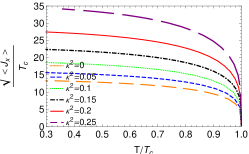
(a)  $b=0$

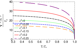
(b)  $b=0.04$

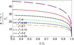
(c)  $b=0.08$

Figure 1: The behavior of condensation parameter as a function of temperature for different values of backreaction.

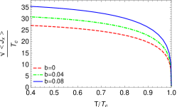
(a)  $\kappa^{2}=0$

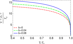
(b)  $\kappa^{2}=0.10$

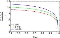
(c)  $\kappa^{2}=0.20$

Figure 2: Plot of condensation as a function of temperature with $m^{2}=1$ for different values of the nonlinearity parameter $b$ .

	$b=0$		$b=0.04$		$b=0.08$
	Analytical	Numerical	Analytical	Numerical	Analytical	Numerical
$\kappa^{2}=0$	$0.0478$	$0.0503$	$0.0416$	$0.0454$	$0.0343$	$0.0406$
$\kappa^{2}=0.05$	$0.0443$	$0.0410$	$0.0379$	$0.0366$	$0.0303$	$0.0324$
$\kappa^{2}=0.1$	$0.0424$	$0.0330$	$0.0361$	$0.0290$	$0.0281$	$0.0254$
$\kappa^{2}=0.15$	$0.0394$	$0.0260$	$0.0331$	$0.0226$	$0.0248$	$0.0195$
$\kappa^{2}=0.2$	$0.0353$	$0.0201$	$0.0291$	$0.0172$	$0.0205$	$0.0146$
$\kappa^{2}=0.25$	$0.0302$	$0.0152$	$0.0241$	$0.0127$	$0.0153$	$0.0106$

Table 1: Analytical and Numerical results of $T_{c}/\mu$ for different values of the backreaction and nonlinear parameters with trial function $F(z)=1-\alpha z^{2}$.

	$b=0$		$b=0.04$		$b=0.08$
	Analytical	Numerical	Analytical	Numerical	Analytical	Numerical
$\kappa^{2}=0$	$0.0466$	$0.0503$	$0.0400$	$0.0454$	$0.0320$	$0.0406$
$\kappa^{2}=0.05$	$0.0397$	$0.0410$	$0.0347$	$0.0366$	$0.0243$	$0.0324$
$\kappa^{2}=0.1$	$0.0375$	$0.0330$	$0.0328$	$0.0290$	$0.0215$	$0.0254$
$\kappa^{2}=0.15$	$0.0342$	$0.0260$	$0.0298$	$0.0226$	$0.0178$	$0.0195$
$\kappa^{2}=0.2$	$0.0296$	$0.0201$	$0.0258$	$0.0172$	$0.0132$	$0.0146$
$\kappa^{2}=0.25$	$0.0238$	$0.0152$	$0.0208$	$0.0127$	$0.0083$	$0.0106$

Table 2: Analytical and Numerical results of $T_{c}/\mu$ for different values of the backreaction and nonlinear parameters with $F(z)=1-\alpha z^{3}$.

	$b=0$		$b=0.04$		$b=0.08$
	Analytical	Numerical	Analytical	Numerical	Analytical	Numerical
$\kappa^{2}=0$	$0.0457$	$0.0503$	$0.0387$	$0.0454$	$0.0303$	$0.0406$
$\kappa^{2}=0.05$	$0.0379$	$0.0410$	$0.0328$	$0.0366$	$0.0205$	$0.0324$
$\kappa^{2}=0.1$	$0.0356$	$0.0330$	$0.0308$	$0.0290$	$0.0171$	$0.0254$
$\kappa^{2}=0.15$	$0.0321$	$0.0260$	$0.0278$	$0.0226$	$0.0131$	$0.0195$
$\kappa^{2}=0.2$	$0.0274$	$0.0201$	$0.0236$	$0.0172$	$0.0084$	$0.0146$
$\kappa^{2}=0.25$	$0.0214$	$0.0152$	$0.0186$	$0.0127$	$0.0039$	$0.0106$

Table 3: Analytical and Numerical results of $T_{c}/\mu$ for different values of the backreaction and nonlinear parameters with $F(z)=1-\alpha z^{4}$.

III condensation of vector field

Let us now investigate the relation between the critical temperature $T_{c}$ and the chemical potential $\mu$ for holographic $p$-wave superconductor. In particular, we would like to explore the effects of backreaction as well as nonlinearity parameter on the critical temperature.

Analytical approach

In order to follow our analytical studies, we apply the Sturm-Liouville eigenvalue problem and define $z=r_{+}/r$ as a new variable where $0\leq z\leq 1$. Therefore, Eqs. (9)-(12) turn to

$$f^{\prime}(z)+\frac{2r_{+}^{2}}{z^{3}}+\frac{2\kappa^{2}}{z}\left[-\rho_{x}{}^{2}(z)-\frac{e^{\chi(z)}\phi^{2}(z)\rho_{x}{}^{2}(z)}{f(z)}-\frac{z^{4}f(z)\rho_{x}^{\prime}{}^{2}(z)}{r_{+}^{2}}+\frac{r_{+}^{2}}{bz^{2}}\left[1-\frac{1}{\sqrt{1-\frac{bz^{4}e^{\chi(z)}\phi^{\prime 2}(z)}{r_{+}^{2}}}}\right]\right]=0,$$ (17)

$$\chi^{\prime}(z)-4\kappa^{2}\left[\frac{e^{\chi(z)}\phi^{2}(z)\rho_{x}{}^{2}(z)}{zf^{2}(z)}+\frac{z^{3}\rho_{x}^{\prime}{}^{2}(z)}{r_{+}^{2}}\right]=0,$$ (18)

$$\phi^{\prime\prime}(z)+\phi^{\prime}(z)\left[\frac{1}{z}+\frac{\chi^{\prime}(z)}{2}+\frac{bz^{3}e^{\chi(z)}\phi^{\prime 2}(z)}{r_{+}^{2}}\right]-\frac{2\phi(z)\rho_{x}^{2}(z)}{z^{2}f(z)}\left[1-\frac{bz^{4}e^{\chi(z)}\phi^{\prime 2}(z)}{r_{+}^{2}}\right]^{3/2}=0,$$ (19)

$$\rho_{x}^{\prime\prime}(z)+\rho_{x}^{\prime}(z)\left[\frac{3}{z}-\frac{\chi^{\prime}(z)}{2}+\frac{f^{\prime}(z)}{f(z)}\right]+\rho_{x}(z)\left[\frac{r_{+}^{2}e^{\chi(z)}\phi^{2}(z)}{z^{4}f^{2}(z)}-\frac{r_{+}^{2}}{z^{4}f(z)}\right]=0.$$ (20)

Here, the prime indicates the derivative with respect to $z$. In the vicinity of the critical temperature the expectation value of $\langle J_{x}\rangle$ is tiny so we take it as an expansion parameter

$$\epsilon\equiv\left\langle J_{x}\right\rangle.$$

We concentrate on the solutions for small values of the condensation parameter $\epsilon$, because near the critical temperature we have $\epsilon\ll 1$. Therefore, we expand the functions in terms of the $\epsilon$ as

$$f\approx f_{0}+\epsilon^{2}f_{2}+\epsilon^{4}f_{4}+\cdots,$$

$$\chi\approx\epsilon^{2}\chi_{2}+\epsilon^{4}\chi_{4}+\cdots,$$

$$\phi\approx\phi_{0}+\epsilon^{2}\phi_{2}+\epsilon^{4}\phi_{4}+\cdots,$$

$$\rho_{x}\approx\epsilon\rho_{x_{1}}+\epsilon^{3}\rho_{x_{3}}+\epsilon^{5}\rho_{x_{5}}+\cdots.$$

Moreover, the chemical potential can be expressed as

$$\mu=\mu_{0}+\epsilon^{2}\delta\mu_{2}+...\rightarrow\epsilon\thickapprox\Bigg{(}\frac{\mu-\mu_{0}}{\delta\mu_{2}}\Bigg{)}^{1/2},\ \ \ \ \delta\mu_{2}>0.$$

Near the phase transition $\mu_{c}=\mu_{0}$, so the order parameter vanishes. In addition, the mean field value for the critical exponent $\beta=1/2$ is obtained.
At zeroth order of $\epsilon$, the equation for the gauge field (19) turns to

$$\phi^{\prime\prime}(z)+\frac{\phi^{\prime}(z)}{z}+\frac{bz^{3}\phi^{\prime 3}(z)}{r_{+}^{2}}=0.$$ (21)

We can find the solution for this equation as fallow

$$\phi(z)=\lambda r_{+}\log(z)-\frac{1}{4}b\lambda^{3}r_{+}\left(z^{2}-1\right),\ \ \ \lambda=\frac{\mu}{r_{+}}.$$ (22)

Substituting solution (22) into Eq. (17), we arrive at

$$f^{\prime}(z)+\frac{2r_{+}^{2}}{z^{3}}+\frac{2\kappa^{2}r_{+}^{2}}{bz^{3}}\left(1-\frac{1}{\sqrt{1-\frac{bz^{4}\phi^{\prime 2}(z)}{r_{+}^{2}}}}\right)=0,$$ (23)

The solution for $f(z)$, at zeroth order of $\epsilon$, can be obtained as

$$f(z)=\frac{r_{+}^{2}g(z)}{z^{2}},\ \ \ \ g(z)=1-z^{2}+\kappa^{2}\lambda^{2}z^{2}\log(z)+\frac{1}{8}b\kappa^{2}\lambda^{4}z^{2}-\frac{1}{8}b\kappa^{2}\lambda^{4}z^{4}.$$ (24)

Near the boundary, we can define the function $\rho_{x}(z)$ based on the trial function $F(z)=1-\alpha z^{\varpi}$ in which $\varpi\geq 2$ and satisfies the boundary conditions $F(0)=1$ and $F^{{}^{\prime}}(0)=0$,

$$\rho_{x}(z)=\frac{\langle J_{x}\rangle}{\sqrt{2}r_{+}^{\Delta}}z^{\Delta}F(z).$$ (25)

Inserting Eqs. (24) and (25) in Eq. (20), we arrive at

$$F^{\prime\prime}(z)+F^{\prime}(z)\left[\frac{g^{\prime}(z)}{g(z)}+\frac{2\Delta}{z}+\frac{1}{z}\right]+F(z)\left[\frac{\Delta g^{\prime}(z)}{zg(z)}-\frac{1}{z^{2}g(z)}+\frac{\Delta^{2}}{z^{2}}\right]-\frac{F(z)\lambda^{2}\log(z)}{2g^{2}(z)}\left[b\lambda^{2}r_{+}\left(z^{2}-1\right)-2\log(z)\right]=0.$$ (26)

The Sturm-Liouville form of this equation is

$$\left[T(z)F^{\prime}(z)\right]^{\prime}+P(z)T(z)F(z)+\lambda^{2}Q(z)T(z)F(z)=0,$$ (27)

where

$$T(z)=z^{2\Delta+1}\left[\left(1-z^{2}\right)\left(1+\frac{b}{8}\kappa^{2}\lambda^{4}z^{2}\right)+\kappa^{2}\lambda^{2}z^{2}\log(z)\right],$$ (28)

$$P(z)=\frac{\Delta}{z}\left(\frac{g^{\prime}(z)}{g(z)}+\frac{\Delta}{z}\right)-\frac{1}{z^{2}g(z)},$$ (29)

$$Q(z)=\frac{\log(z)}{g^{2}(z)}\left[\log(z)+\frac{b}{2}\lambda^{2}r_{+}\left(1-z^{2}\right)\right].$$ (30)

According to the Sturm-Liouville eigenvalue problem, we should minimize the following expression with respect to $\alpha$.

$$\lambda^{2}=\frac{\int_{0}^{1}T\left(F^{\prime 2}-PF^{2}\right)dz}{\int_{0}^{1}TQF^{2}dz},$$ (31)

The definition of the backreaction parameter, based on the iteration method, is LPJW2015

$$\kappa_{n}=n\Delta\kappa,\ \ \ n=0,1,2,\cdots,\ \ \Delta\kappa=\kappa_{n+1}-\kappa_{n}.$$ (32)

where we take $\Delta\kappa=0.05$. In addition, we have

$$\kappa^{2}\lambda^{2}={\kappa_{n}}^{2}\lambda^{2}={\kappa_{n}}^{2}(\lambda^{2}|_{\kappa_{n-1}})+O[(\Delta\kappa)^{4}],\ \ \kappa_{-1}=0,\ \ \lambda^{2}|_{\kappa_{-1}}=0,$$ (33)

$$b\lambda^{2}=b\left(\lambda^{2}|_{b=0}\right)+\mathcal{O}(b^{2}).$$ (34)

Using Eqs. (8) and (9), the critical temperature, at zeroth order with respect to $\epsilon$, is given by

$$T_{c}=\frac{f^{\prime}\left(r_{+c}\right)}{4\pi}=\frac{r_{+c}}{4\pi}\left[2-\kappa^{2}\lambda^{2}+\frac{1}{4}b\kappa^{2}\lambda^{4}\right]=\frac{1}{4\pi}\left(\frac{\mu}{\lambda}\right)\left[2-\kappa_{n}^{2}(\lambda^{2}|_{\kappa_{n-1}})+\frac{1}{4}b\kappa_{n}^{2}(\lambda^{4}|_{\kappa_{n-1},b=0})\right].$$ (35)

Considering three different forms of the trial function $F(z)$, the analytical results of $T_{c}/\mu$ affected by different values of backreaction and nonlinear parameters are listed in tables I, II and III. Based on these results, the effects of increasing the backreaction parameter $\kappa$ for a fixed values of nonlinear parameter $b$ are the same as increasing the nonlinear parameter for a fixed value of $\kappa$. In other words, in both cases, the value of $T_{c}/\mu$ decreases by increasing the backreaction or nonlinear parameters. Thus, the presence of backreaction and BI nonlinear electrodynamics makes the vector hair harder to form. In addition, for the case with $b=0$, the results of mahyap for $T_{c}/\mu$ are reproduced.

Numerical solution

To do our numerical solution for the $(1+1)$-dimension holographic $p$-wave superconductor in the presence of backreaction and BI nonlinear electrodynamics, we employ the shooting method. For this purpose, we need to know the behavior of the equations of motion (19)-(18) both at horizon and boundary. We use the facts that $\phi(z=1)=0$, otherwise the norm of the gauge field $A_{\mu}$ will be ill-defined at the horizon where $f(z=1)=0$. By using these conditions, we can expand the metric functions and vector field, around $z=1$, as

$$f(z)=f_{1}\left(1-z\right)+f_{2}\left(1-z\right){}^{2}+\cdots,$$ (36)

$$\chi(z)=\chi_{0}+\chi_{1}\left(1-z\right)+\chi_{2}\left(1-z\right){}^{2}+\cdots,$$ (37)

$$\phi(z)=\phi_{1}\left(1-z\right)+\phi_{2}\left(1-z\right){}^{2}+\cdots,$$ (38)

$$\rho_{x}(z)=\rho_{x_{0}}+\rho_{x_{1}}\left(1-z\right)+\rho_{x_{2}}\left(1-z\right){}^{2}+\cdots.$$ (39)

The higher orders will be disregarded because in the vicinity of horizon $(1-z)^{n}$ is very small and can be neglected. In this method, we can write all coefficients in terms of $\phi_{1}$, $\rho_{x_{0}}$ and $\chi_{0}$. By varying these three parameters at the horizon, we try to gain the desirable state $\rho_{x_{-}}(\infty)=\chi(\infty)=0$. In addition, we can set $r_{+}=1$ by virtue of the equations of motion’s symmetry

$$r\rightarrow ar,\text{ \ \ \ \ }f\rightarrow a^{2}f,\text{ \ \ \ \ }\phi\rightarrow a\phi.$$

Consequently, the numerical values of $T_{c}/\mu$ for different values of backreaction and nonlinearity parameters are achieved. In order to show that there is a good agreement between analytical and numerical results, we present the numerical results in tables I, II and III, too. However, we observe differences in results in some cases which originates from the fact that in order to solve the analytical solution, we use some simplifications. One may argue that these disagreements could be solved by considering the polynomial in the form of $F(z)=1-\alpha z^{2}-\beta z^{3}-\gamma z^{4}$, as the trial function. However, in this case one faces with difficulties to achieve the solutions for larger values of the BI and backreaction parameters. Indeed, in this case, besides finding the parameter $\alpha$, we have to find $\beta$ and $\gamma$ parameters. Actually, the analytical method in holographic p-wave superconductors is very difficult. And for this reason, most studies on the holographic p-wave superconductors have been carried out numerically. In addition, the investigation of one dimensional holographic superconductors in the background of three dimensional BTZ black hole is a difficult problem due to the logarithmic behavior of the gauge field $\phi$. Overall, the shooting method’s results follow the same trend as the results of the Sturm-Liouville method, namely, by increasing the strength of backreaction as well as the nonlinearity parameters for each form of the trial function $F(z)$. Indeed, increasing the value of backreaction and nonlinear parameters, makes the condensation much harder to form. In addition for $b=0$, the numerical values of mahyap are regained. Figures 1 and 2 show, respectively, the behavior of condensation as a function of temperature for different values of backreaction and nonlinear parameters. Based on these figures, the condensation gap increases for larger values of the backreaction and nonlinearity parameters, while the other one is fixed. This implies that it is harder to form a holographic $p$-wave superconductor in the presence of backreaction and BI nonlinear parameters.

IV Critical exponents

In this section, we are going to calculate the expectation value of $\langle J_{x}\rangle$ in the vicinity of the critical temperature $T_{c}$ for the one-dimensional holographic $p$-wave superconductor developed in a BTZ black hole background, when the gauge and vector fields backreact on the background geometry in the presence of BI nonlinear electrodynamics. Again, we do our calculations both analytically and numerically.

Analytical study

To follow the analytical approach, we consider the behavior of gauge field $A_{\mu}$ near the critical temperature. Since the condensation in the vicinity of the critical temperature is nonzero, we expect to have an extra term in the consequent equation compared to the field equation (21) in the previous section. Thus, Eq. (19) turns to

$$\phi^{\prime\prime}(z)+\frac{\phi^{\prime}(z)}{z}+\frac{bz^{3}\phi^{\prime 3}(z)}{r_{+}^{2}}-\frac{2\phi(z)\rho_{x}{}^{2}(z)}{z^{2}f(z)}\left(1-\frac{bz^{4}}{r_{+}^{2}}\phi^{\prime 2}(z)\right)^{3/2}=0.$$ (40)

Substituting Eqs. (24) and (25) in the above expression, we get

$$\phi^{\prime\prime}(z)+\frac{\phi^{\prime}(z)}{z}+\frac{bz^{3}\phi^{\prime 3}(z)}{r_{+}^{2}}=\frac{\langle J_{x}\rangle^{2}}{r_{+}^{4}}\phi(z)\Xi(z),$$ (41)

where

$$\Xi(z)=\frac{z^{2}F^{2}(z)}{g(z)}\left(1-\frac{3bz^{4}\phi^{\prime 2}(z)}{2r_{+}^{2}}\right).$$ (42)

In order to find the solution of Eq. (41), we note that near the critical temperature, $T\simeq T_{c}$, the value of ${\langle J_{x}\rangle^{2}}/{r_{+}^{4}}$ is small, so we may write the solution in the form

$$\frac{\phi(z)}{r_{+}}=\lambda\log(z)-\frac{1}{4}b\lambda^{3}\left(z^{2}-1\right)+\frac{\langle J_{x}\rangle^{2}}{r_{+}^{4}}\eta(z).$$ (43)

At the horizon $\phi(z=1)=0$ we have $\eta(1)=0$. Substituting Eq. (43) in Eq. (41) we arrive at

$$\eta^{\prime\prime}(z)+\frac{\eta^{\prime}(z)}{z}+3bz\lambda^{2}\eta^{\prime}(z)=\frac{\lambda z^{2}F^{2}(z)}{g(z)}\left[\log(z)-\frac{1}{4}b\lambda^{2}\left(z^{2}-1\right)-\frac{3}{2}b\lambda^{2}z^{2}\log(z)\right].$$ (44)

Multiplying both sides of Eq. (44) by factor $ze^{\frac{3}{2}b\lambda^{2}z^{2}}$, we get

$$\int_{0}^{1}d(ze^{\frac{3}{2}b\lambda^{2}z^{2}}\eta^{\prime}(z))=e^{\frac{3b\lambda^{2}}{2}}\eta^{\prime}(1)=\lambda\mathcal{A},$$ (45)

where

$$\mathcal{A}=\int_{0}^{1}\frac{z^{3}}{g(z)}F^{2}(z)e^{\frac{3}{2}b\lambda^{2}z^{2}}\left[\log(z)-\frac{1}{4}b\lambda^{2}\left(z^{2}-1\right)-\frac{3}{2}b\lambda^{2}z^{2}\log(z)\right]\,dz.$$ (46)

Now, we use the coordinate transformation $z\rightarrow Z+1$ in Eq. (22). Considering the fact that the first term on the rhs of Eq. (43) is the solution of $\phi(z)$ at the critical point, and the second term is a correction term, we have

$$\frac{\rho}{r_{+}}+\frac{\mu}{r_{+}}\log(1+Z)=\frac{\mu}{r_{+c}}\log(1+Z)-\frac{1}{4}b\left(\frac{\mu}{r_{+c}}\right)^{3}\left[(1+Z)^{2}-1\right]+\frac{\langle J_{x}\rangle^{2}}{r_{+c}^{4}}\eta(1+Z),$$ (47)

Then, by expanding the resulting equation around $Z=0$ we find

$$\frac{\rho}{r_{+}}+\frac{\mu}{r_{+}}\left(Z-\frac{Z^{2}}{2}+...\right)=\frac{\mu}{r_{+c}}\left(Z-\frac{Z^{2}}{2}+...\right)-\frac{1}{4}b\left(\frac{\mu}{r_{+c}}\right)^{3}\left[(1+Z)^{2}-1\right]+\frac{\langle J_{x}\rangle^{2}}{r_{+c}^{4}}\left(\eta(1)+Z\eta^{\prime}(1)+...\right).$$ (48)

Comparing the coefficients $Z$ on both sides of Eq. (48) and using Eq. (45) we find

$$\frac{\mu}{r_{+}}=\frac{\mu}{r_{+c}}\left(1+\frac{\langle J_{x}\rangle^{2}}{r_{+c}^{4}}\mathcal{A}e^{-\frac{3}{2}b\lambda^{2}}\right),$$ (49)

Near the critical point we have $T\sim T_{c}$, and thus using relation (35), we can find $r_{+}$ as

$$r_{+}=\frac{4\pi T}{\left(2-\kappa^{2}\lambda^{2}+\frac{1}{4}b\kappa^{2}\lambda^{4}\right)}.$$ (50)

Inserting Eqs. (35) and (50) in Eq. (49) and taking the absolute values of the resulting equation, we arrive at

$$\langle J_{x}\rangle=\gamma T_{c}^{2}\sqrt{1-\frac{T}{T_{c}}},$$ (51)

where

$$\gamma=\frac{1}{\sqrt{\left|\mathcal{A}\right|}}\left(\frac{4\pi}{2-\kappa^{2}\lambda^{2}+\frac{1}{4}b\kappa^{2}\lambda^{4}}\right)^{2}e^{\frac{3}{4}b\lambda^{2}}.$$ (52)

According to this equation, the critical exponent $\beta=1/2$ is in good agreement with the mean field theory. We face with the second order phase transition for all values of the backreaction and nonlinear parameters because the value of $\beta$ is independent of the effect of backreaction and nonlinearity. In addition, the equation (52) for $b\rightarrow 0$ turns to equivalent equation in mahyap .

Numerical approach

Using the results of analytical solution for the condensation in the vicinity of the critical temperature (i.e. equation (51)) we have

$$\log\left(\frac{\langle J_{x}\rangle}{T_{c}^{2}}\right)=\log(\gamma)+\frac{1}{2}\log\left(1-\frac{T}{T_{c}}\right).$$ (53)

Figures 3 and 4 give information about the behavior of $\log\left(\frac{\langle J_{x}\rangle}{T_{c}^{2}}\right)$ as a function of $\log\left(1-\frac{T}{T_{c}}\right)$ in the presence of backreaction and BI nonlinear parameters. The slope of curves is $1/2$ which is in agreement with analytical approach. In addition, both methods follow the mean field theory and the second order phase transition is occurred.

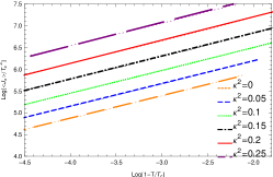
(a)  $b=0$

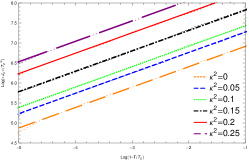
(b)  $b=0.04$

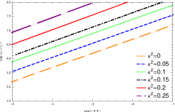
(c)  $b=0.08$

Figure 3: The behavior of $\log\langle J_{x}\rangle/T_{c}^{2}$ as a function of $\log(1-T/T_{c})$ with slope of $1/2$ for different values of backreaction parameters.

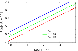
(a)  $\kappa^{2}=0$

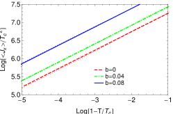
(b)  $\kappa^{2}=0.10$

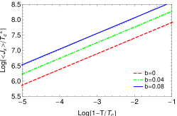
(c)  $\kappa^{2}=0.20$

Figure 4: The behavior of $\log\langle J_{x}\rangle/T_{c}^{2}$ as a function of $\log(1-T/T_{c})$ with slope of $1/2$ for different values of nonlinearity parameters.

V Conductivity

In this section, we obtain the electrical conductivity as a function of frequency for the one-dimensional holographic $p$-wave superconductors in the presence of backreaction and BI nonlinear electrodynamics by applying appropriate electromagnetic perturbations of $A_{x}$ and $g_{tx}$ on the black hole background. Based on the AdS/CFT correspondence, these perturbations in the bulk are dual to the boundary electric current. If we consider $\sigma_{ij}$ and $J_{i}$ as the electric conductivity and external electric field, according to the Ohm’s law we have

$$\sigma_{ij}=\frac{J_{i}}{E_{j}}.$$ (54)

In order to calculate the conductivity in $x$-direction we need to add the following perturbational terms in the bulk gauge potential and metric

$$\delta A_{x}=A_{x}(r)e^{-i\omega t},\ \ \ \delta g_{tx}=g_{tx}(r)e^{-i\omega t}.$$ (55)

Using Eq. (55), the linearized form of $x$-component of the electromagnetic equation (4) turns to

$$A_{x}^{\prime\prime}(r) + A_{x}^{\prime}(r)\left[\frac{f^{\prime}(r)}{f(r)}-\frac{\chi^{\prime}(r)}{2}-\frac{1}{r}+\frac{2b\rho_{x}^{2}(r)e^{\chi(r)}\phi(r)\phi^{\prime}(r)}{r^{2}f(r)}\sqrt{1-be^{\chi(r)}\phi^{\prime 2}(r)}-\frac{be^{\chi(r)}\phi^{\prime 2}(r)}{r}\right]$$ (56)

$$+ A_{x}(r)\frac{\omega^{2}e^{\chi(r)}}{f^{2}(r)}+\frac{e^{\chi(r)}\phi^{\prime}(r)}{f(r)}\left[g_{tx}^{\prime}(r)-\frac{2g_{tx}(r)}{r}\right]+\frac{2\rho_{x}^{2}(r)e^{\chi(r)}\phi(r)}{r^{2}f^{2}(r)}g_{tx}(r)\sqrt{1-be^{\chi(r)}\phi^{\prime 2}(r)}=0.$$

Also, using $(tt),(xx),(tx),(xt),(xr)$-components of the Einstein equations and after some simplification, we arrive at

$$\frac{1}{2\kappa^{2}}\left[g_{tx}^{\prime}(r)-\frac{2g_{tx}(r)}{r}\right]+\frac{A_{x}(r)\phi^{\prime}(r)}{\sqrt{1-be^{\chi(r)}\phi^{\prime 2}(r)}}=0,$$ (57)

$$\frac{2}{r^{2}}A_{x}(r)\rho_{x}^{2}(r)+\frac{2\rho_{x}^{2}(r)e^{\chi(r)}\phi(r)}{r^{2}f(r)}g_{tx}(r)=0.$$ (58)

Substituting Eqs. (57) and (58) in Eq.(56), we obtain the linearized equation for the gauge field $A_{x}$

$$A_{x}^{\prime\prime}(r) + A_{x}^{\prime}(r)\left[\frac{f^{\prime}(r)}{f(r)}-\frac{\chi^{\prime}(r)}{2}-\frac{1}{r}+\frac{2b\rho_{x}^{2}(r)e^{\chi(r)}\phi(r)\phi^{\prime}(r)}{r^{2}f(r)}\sqrt{1-be^{\chi(r)}\phi^{\prime 2}(r)}-\frac{be^{\chi(r)}\phi^{\prime 2}(r)}{r}\right]$$ (59)

$$+ A_{x}(r)\left[\frac{\omega^{2}e^{\chi(r)}}{f^{2}(r)}-\frac{2\rho_{x}^{2}(r)}{r^{2}f(r)}\sqrt{1-be^{\chi(r)}\phi^{\prime 2}(r)}-\frac{2\kappa^{2}e^{\chi(r)}\phi^{\prime 2}(r)}{f(r)\sqrt{1-be^{\chi(r)}\phi^{\prime 2}(r)}}\right]=0.$$

Let us note that, of course, investigating the effects of nonlinearity as well as the backreaction parameters on the conductivity is a worthy task. However in order to compute the conductivity in the holographic approach in the presence of nonlinear and backreaction parameters, we need to turn on the one component of the gauge field as well as the metric. This extra component makes the calculations too difficult and we face with difficulty in numerical solutions for the cases with nonzero values of backreaction. Therefore, for simplicity, in what follows, we consider only the probe limit by setting $g_{tx}(r)=0=\chi(r)$ in the presence of BI nonlinear electrodynamics. Thus, in the absence of backreaction, Eq. (56) can be written as

$$A_{x}^{\prime\prime}(r)+A_{x}^{\prime}(r)\left[\frac{f^{\prime}(r)}{f(r)}-\frac{1}{r}+\frac{2b\rho_{x}^{2}(r)\phi(r)\phi^{\prime}(r)}{r^{2}f(r)}\sqrt{1-b\phi^{\prime 2}(r)}-\frac{b\phi^{\prime 2}(r)}{r}\right]+\frac{\omega^{2}A_{x}(r)}{f^{2}(r)}=0,$$ (60)

where it admits the asymptotic solution in the following form

$$A_{x}=A_{x}^{(0)}+A_{x}^{(1)}\log\left(\frac{1}{r}\right).$$ (61)

Based on the AdS/CFT dictionary, $A_{x}^{(0)}$ plays the role of the source in the dual theory, while $A_{x}^{(1)}$ will give the expectation value of the dual current. For the boundary current we have

$$J=\frac{\text{$\delta$S}_{\text{bulk}}}{\text{$\delta$A}^{(0)}}=\frac{\text{$\delta$S}_{o.s}}{\text{$\delta$A}^{(0)}}=\frac{\partial(\sqrt{-g}\mathcal{L}_{m})}{\partial A_{x}^{\prime}}|r\rightarrow\infty,$$ (62)

where

$$S_{o.s.}=\int_{r_{+}}^{\infty}\,dr\int\,{d}^{2}x\sqrt{-g}\mathcal{L}_{m}.$$ (63)

Integrating by parts and using Eq. (60), we get

$$S_{o.s.}=\int\,{d}^{2}x\frac{f(r)A_{x}(r)A_{x}^{\prime}(r)}{2r\left(1-b\phi^{\prime 2}(r)\right)}.$$ (64)

Using the asymptotic behavior of $\phi(r)$, $f(r)$ and $A_{x}(r)$ given by Eqs. (16) and (61), we can calculate $J_{x}$. So, the electrical conductivity based on the equation (54) is

$$\sigma(\omega)=\frac{J_{x}}{E_{x}}=-\frac{iA_{x}^{(1)}}{\omega A_{x}^{(0)}}=-\frac{izA_{x}^{\prime}(z)}{\omega\left[A_{x}(z)-zA_{x}^{\prime}(z)\log(z)\right]},$$ (65)

where

$$E_{x}=-\partial_{t}\delta A_{x}.$$ (66)

Following the analytical approach to calculate conductivity seems difficult thus we apply the numerical method. In order to do that, we consider ingoing wave boundary condition in the vicinity of the horizon for $A_{x}(r)$ as follow

$$A_{x}(r)=f(r)^{\frac{-i\omega}{4\pi T}}\left[1+a(1-r)+b(1-r)+\cdots\right].$$ (67)

In the above equation, $T$ is the Hawking temperature which in the probe limit $T=r_{+}/(2\pi)$ because in this case $f(r)=r^{2}-1$. Furthermore, $a$, $b$, $\cdots$ are obtained based on the Taylor expansion of equation (60) around horizon. Now, due to Eq. (65) we can numerically explore the behavior of the conductivity for the $(1+1)$-dimensional holographic $p$-wave superconductor in the probe limit in presence of BI nonlinear electrodynamics. Figures 5 and 6 give information about the behavior of the real and imaginary parts of conductivity as a function of $\omega/T$ for different values of nonlinearity parameter $b$ in the case $\kappa^{2}=0$ for $T/T_{c}=0.2,0.5,0.8$. Delta function in the real part of the conductivity isn’t related to imaginary part near $\omega/T=0$ by the Kramers-Kronig relation because imaginary part tends to zero instead of having a pole in this region. In addition, $Re\sigma(\omega)$ tends to zero value at high frequency same as Bu . The imaginary and real parts of conductivity follow a different trend in higher dimensions because we face with the absence of gap and divergence behavior in real and imaginary parts, respectively. Moreover, the effect of different values of temperature is more apparent for larger values of nonlinearity parameter. Figures 7 and 8 show the effect of different values of nonlinearity parameter $b$ for fixed values of $T/T_{c}$. Based on these figures, the difference of graphs becomes more obvious by increasing the value of $T/T_{c}$. In addition, for the fixed value of $T/T_{c}$ strengthen the effect of nonlinearity makes Drude-like peak in real part of conductivity to increase and causes deeper minimum values in imaginary part.

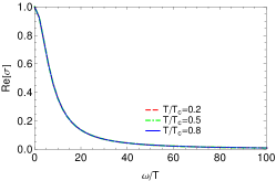
(a)  $b=0$

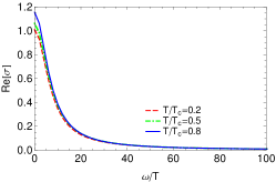
(b)  $b=0.04$

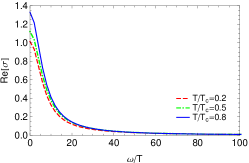
(c)  $b=0.08$

Figure 5: The behavior of real part of conductivity as a function of $\omega/T$ for different values of temperature in the case $\kappa^{2}=0$.

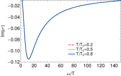
(a)  $b=0$

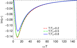
(b)  $b=0.04$

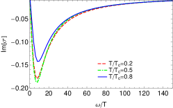
(c)  $b=0.08$

Figure 6: The behavior of imaginary part of conductivity as a function of $\omega/T$ for different values of temperature in the case $\kappa^{2}=0$.

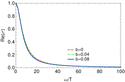
(a)  $T/T_{c}=0.2$

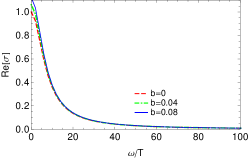
(b)  $T/T_{c}=0.5$

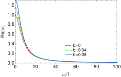
(c)  $T/T_{c}=0.8$

Figure 7: The behavior of real part of conductivity as a function of $\omega/T$ for different values of $b$ in the case $\kappa^{2}=0$.

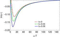
(a)  $T/T_{c}=0.2$

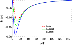
(b)  $T/T_{c}=0.5$

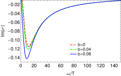
(c)  $T/T_{c}=0.8$

Figure 8: The behavior of imaginary part of conductivity as a function of $\omega/T$ for different values of $b$ in the case $\kappa^{2}=0$.

VI summary and discussion

We have investigated one-dimensional holographic $p$-wave superconductor model by applying $AdS3/CFT2$ when the gauge and vector fields backreact on the background geometry in the presence of BI nonlinear electrodynamics. For this purpose, we employ the Sturm-Liouville eigenvalue problem for analytical investigations and the shooting method for the numerical calculations. In both methods, we find the relation between the critical temperature $T_{c}$ and the chemical potential $\mu$ for different values of the nonlinear and backreaction parameters. The results of analytical and numerical methods are in good agreement with each other. We found out that increasing the values of the nonlinearity and backreaction parameters decrease the critical temperature and thus makes the condensation harder to form. Furthermore, critical exponent of this system were also obtained both analytically and numerically. We face with a second order phase transition with $\beta=1/2$ which follows the mean field theory. This value is independent of backreaction and nonlinear effects.

In addition, we analyzed the conductivity of this system for the case of probe limit and investigated the properties of real and imaginary parts of conductivity for different values of the nonlinear parameter $b$. The behavior of both real and imaginary parts of conductivity are so different from higher dimensions and they don’t connect to each other based on the Kramers-Kronig relation. We don’t observe divergency near $\omega/T=0$ in the imaginary part of the conductivity where a delta function in the real part appears. By increasing the effect of nonlinearity, we obtain larger values for Drude-like peak in real part of conductivity and deeper minimum values of imaginary part. It’s difficult to see the effect of different temperatures for small values of nonlinearity parameter. However, the effect of temperature becomes apparent by increasing the $b$.