The Open Porous Media Flow Reservoir Simulator

Abstract

The Open Porous Media (OPM) initiative is a community effort that encourages open innovation and reproducible research for simulation of porous media processes. OPM coordinates collaborative software development, maintains and distributes open-source software and open data sets, and seeks to ensure that these are available under a free license in a long-term perspective.

In this paper, we present OPM Flow, which is a reservoir simulator developed for industrial use, as well as some of the individual components used to make OPM Flow. The descriptions apply to the 2019.10 release of OPM.

1 Introduction

The Open Porous Media (OPM) initiative was started in 2009 to encourage open innovation and reproducible research on modelling and simulation of porous media processes. OPM was initially founded as a collaboration between groups at Equinor (formerly Statoil), SINTEF, the University of Stuttgart, and the University of Bergen, but over time, several other groups and individuals have joined and contributed. What today forms the OPM suite of software, has mainly been developed by SINTEF, NORCE (formerly IRIS), Equinor, Ceetron Solutions, Poware Software Solutions, and Dr. Blatt HPC-Simulation-Software & Services.

The initial vision was to create long-lasting, efficient, and well-maintained, open-source software for simulating flow and transport in porous media. The scope has later been extended to also provide open data sets, thus making it easier to benchmark, compare, and test different mathematical models, computational methods, and software implementations.

Figure 1: Current module structure as of the 2019.10 release. Arrows indicate inter-module dependencies: a module depends on another module if it has an arrow pointing towards it. Since the OPM software suite is in active development, the module organization is likely to keep changing in the future.

OPM has so far primarily focussed on tools for reservoir simulation, and consists today of the OPM Flow reservoir simulator, upscaling tools, and a selection of supporting and experimental software pieces. The corresponding source code is divided into six modules, as shown in Figure 1, and is organized as a number of git repositories hosted on github.com/OPM. The data repositories opm-data and opm-tests are also hosted there, and contain example cases and data used for integration testing. Herein, we only give an in-depth description of OPM Flow, which in turn uses or builds on existing frameworks and libraries such as Dune [1], DuMuX [2], Zoltan [3], and Boost to reduce implementation and maintenance cost and improve software quality. The Matlab Reservoir Simulation Toolbox [4, 5, 6] has also been a significant source of ideas and concepts. In addition to the simulator tools, OPM contains the ResInsight postprocessor, which has been used for all the 3D visualization herein. Apart from computational routines underlying flow diagnostics [7], ResInsight is independent of the other OPM modules.

All software in OPM is distributed under the GNU General Public License (GPL), version 3, with the option of using newer versions of the license. Datasets are distributed under the Open Database License, version 1.0, with individual content under the Database Contents License, version 1.0.

Code development in OPM follows an open model: All source code contributions are made using the GitHub pull request mechanism. Anyone can create such a request, which asks the maintainers to merge some change (bugfix, improvement, or new feature) into the master branch of one of the module repositories. Each request is reviewed and typically merged by the maintainer after some discussion and possible revisions of the proposed changes. OPM generally accepts contributions of many kinds, not just software improvements and additions, but also use-case reports, documentation, and bug reports.

2 OPM Flow

OPM Flow is developed to serve two main purposes: 1) as an open-source alternative and drop-in replacement for contemporary commercial simulators to assist oil companies in planning and managing (conventional) hydrocarbon assets, and 2) as a research and prototyping platform that enables its users to implement, test, and validate new models and computational methods in a realistic and industry-relevant setting. To this end, OPM Flow aims to represent reservoir geology, fluid behaviour, and description of wells and production facilities as in commercial simulators and hence offers standard fully-implicit discretizations of black-oil type models and supports industry-standard input and output formats. The simulator is implemented using automatic differentiation (AD) [8] to avoid error-prone derivation and coding of analytical Jacobians for the residual equations, which also makes it easier to extend the simulator with new model equations, e.g., for CO₂ injection or enhanced oil recovery (EOR). Equally important, using AD makes it realtively simple to extend the simulator to compute sensitivities and gradients with respect to various types of model parameters, using e.g., an adjoint method [9].

This paper does not aim to explain how to install or run OPM Flow. For that we refer to the web site, opm-project.org, or the OPM Flow manual [10].

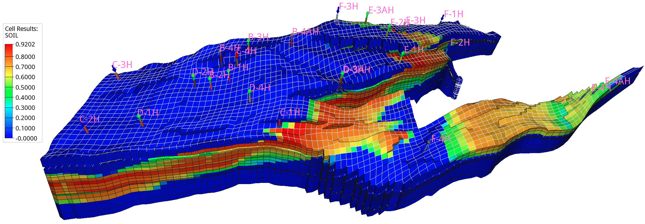
Figure 2: The Norne reservoir showing oil saturation and wells after approximately 3.5 years of production. The z-direction has been exaggerated 5 times.

2.1 The black-oil model

The black-oil equations constitute the most widely used flow model in simulation of hydrocarbon reservoirs. The model is based on the premise that we have three different fluid phases (aqueous, oleic, and gaseous) and three (pseudo)components: water, oil, and gas. Oil and gas are not single hydrocarbon species, but represent all hydrocarbon species that exist in liquid and vapor form at suface conditions. Mixing is allowed, in the sense that both oil and gas can be found in the oleic phase, in the gaseous phase, or in both. The amounts of dissolved gas in the oleic phase and vaporized oil in the gaseous phase must be kept track of. Below, we will use subscripts $w,o,g$ to indicate quantities related to each of the phases or components.

2.1.1 Model equations

The black-oil equations can be deduced from conservation of mass for each component with suitable closure relationships such as Darcy’s law and initial and boundary conditions. The equations are discretized in space with an upwind finite-volume scheme using a two-point flux approximation and in time using an implicit (backward) Euler scheme. The resulting equations are solved simultaneously in a fully implicit formulation by a Newton-type linearization with a properly preconditioned, iterative linear solver. We give both the continuous and discrete equations.

Continuous equations

The conservation laws form a system of partial differential equations, one for each pseudocomponent $\alpha$:

$$\frac{\partial}{\partial t}\left(\phi_{\rm ref}A_{\alpha}\right)+\nabla\cdot{\bf u}_{\alpha}+q_{\alpha} =0,$$ (1)

where the accumulation terms and fluxes are given by

$$A_{w} =m_{\phi}b_{w}s_{w}, {\bf u}_{w} =b_{w}{\bf v}_{w},$$ (2a)

$$A_{o} =m_{\phi}(b_{o}s_{o}+r_{og}b_{g}s_{g}), {\bf u}_{o} =b_{o}{\bf v}_{o}+r_{og}b_{g}{\bf v}_{g},$$ (2b)

$$A_{g} =m_{\phi}(b_{g}s_{g}+r_{go}b_{o}s_{o}), {\bf u}_{g} =b_{g}{\bf v}_{g}+r_{go}b_{o}{\bf v}_{o}.$$ (2c)

and the phase fluxes are given by Darcy’s law:

$${\bf v}_{\alpha}=-\lambda_{\alpha}{\bf K}(\nabla p_{\alpha}-\rho_{\alpha}{\bf g}).$$ (3)

In addition, the following closure relations should hold:

$$s_{w}+s_{o}+s_{g} =1,$$ (4)

$$p_{c,ow} =p_{o}-p_{w},$$ (5)

$$p_{c,og} =p_{o}-p_{g};$$ (6)

see A.1 for definitions of the symbols used.

Discrete equations

In the following, let subscript $i$ denote a discrete quantity defined in cell $i$ and subscript $ij$ denote a discrete quantity defined at the connection between two cells $i$ and $j$. Two cells share a connection if they are adjacent geometrically in the computational grid or share an explicit non-neighbor connection (NNC; provided by the user). For example $v_{o,ij}$ is the oil flux from cell $i$ to cell $j$. For oriented quantities such as fluxes, the orientation is taken to be from cell $i$ to cell $j$, and the quantity is skew-symmetric ($v_{o,ij}=-v_{o,ji}$), whereas non-oriented quantities such as the transmissibility $T_{ij}$ are symmetric ($T_{ij}=T_{ji}$). Quantities with superscript 0 are taken at the start of the discrete time step, other quantities are at the end of the time step. Superscripts or subscripts applied to an expression in parenthesis apply to each element in the expression.

The discretized equations and residuals are, for each pseudo-component $\alpha$ and cell $i$:

$$R_{\alpha,i}=\frac{\phi_{{\rm ref},i}V_{i}}{\Delta t}\left(A_{\alpha,i}-A_{\alpha,i}^{0}\right)+\sum_{j\in C(i)}u_{\alpha,ij}+q_{\alpha,i} =0,$$ (7)

where $A_{\alpha}$ are as in (2) and $u_{\alpha}$ are fluxes defined similar to the velocities ${\bf u}_{\alpha}$:

$$u_{w} =b_{w}v_{w},$$ (8a)

$$u_{o} =b_{o}v_{o}+r_{og}b_{g}v_{g},$$ (8b)

$$u_{g} =b_{g}v_{g}+r_{go}b_{o}v_{o}.$$ (8c)

The relations (4), (5) and (6) hold for each cell $i$. The fluxes are given for each connection $ij$ by:

$$(b_{\alpha}v_{\alpha})_{ij} =(b_{\alpha}\lambda_{\alpha}m_{T})_{U(\alpha,ij)}T_{ij}\Delta\Phi_{\alpha,ij}$$ (9)

$$(r_{\beta\alpha}b_{\alpha}v_{\alpha})_{ij} =(r_{\beta\alpha}b_{\alpha}\lambda_{\alpha}m_{T})_{U(\alpha,ij)}T_{ij}\Delta\Phi_{\alpha,ij}$$ (10)

$$\Delta\Phi_{\alpha,ij} =p_{\alpha,i}-p_{\alpha,j}-g\rho_{\alpha,ij}(z_{i}-z_{j})$$ (11)

$$\rho_{\alpha,ij} =(\rho_{\alpha,i}+\rho_{\alpha,j})/2$$ (12)

$$U(\alpha,ij) =\begin{cases}i,&\Delta\Phi_{\alpha,ij}\geq 0,\\ j,&\Delta\Phi_{\alpha,ij}<0.\\ \end{cases}$$ (13)

See A.2 for definitions of the symbols used above.

2.1.2 Choice of primary variables

For a grid with $n$ cells, the material balances (7) give us $3n$ equations. (When only two phases are defined, either oil/water or oil/gas, the system is simplified and we solve only two mass balance equations, giving 2n equations.) In addition, we have equations and unknowns from the well model, which will be described in Section 2.2. An important question is which quantities we should use as primary variables, i.e., the unknowns we solve for. There is some flexibility, as we have relations connecting many of the quantities.

Our basic choice for non-miscible flow is to use the pressure of one of the phases (which we take to be oil pressure $p_{o}$), $s_{w}$, and $s_{g}$ as our primary variables. The pressure $p_{o}$ will then behave mostly in an elliptic fashion, whereas the saturations $s_{w}$ and $s_{g}$ are more hyperbolic.

For miscible flow, it is a little more complicated: Since the gaseous phase may disappear if all the gas dissolves into the oleic phase, and similarly the oleic phase may disappear if all the oil vaporizes into the gaseous phase, we cannot always use $s_{g}$ for our third variable. Instead we use the third variable to track the composition of the phase that has not disappeared. We therefore use either $s_{g}$, $r_{go}$, or $r_{og}$ as our third primary variable, depending on the fluid state, and we call that variable $x$:

$$x=\begin{cases}s_{g},&\text{all three phases present},\\ r_{go},&\text{no gaseous phase},\\ r_{og},&\text{no oleic phase}.\\ \end{cases}$$ (14)

This choice is made separately for each cell $i$ depending on its state.

2.1.3 Initial and boundary conditions

Initial conditions are defined by the initial values of pressure $p$, saturations $s_{\alpha}$, and, if applicable, the mixing ratios $r_{go}$ and $r_{og}$. These values can be specified by the user directly in the input data, or computed from an equilibration procedure that ensures the initial state is in vertical equilibrium. This procedure takes as input the fluid pressure at a reference depth, the depths of the water-oil and oil-gas contacts, and the capillary pressures at those contact depths. It then solves the following ordinary differential equations:

$$\frac{\mathrm{d}p_{\alpha}}{\mathrm{d}z}=\rho_{\alpha}(z,p_{\alpha})\,g.$$ (15)

The fluid density typically depends on the pressure, and possibly also on its composition; see Section 2.1.6 for details. The equations are solved numerically using a 4th-order Runge-Kutta method, with the order of the phases decided by the location of the datum depth: First, we solve for the phase in whose zone the datum is located, using the datum pressure to fixate the pressure solution. We then solve for phases corresponding to the zones above and below. To fixate the phase pressures, we use the already computed phase pressure(s) evaluated at the zone contact depth and the input capillary pressures.

Good estimates of the initial water saturation of the reservoir are often known from seismic and well logs. This data can be used to improve the initial state. The equilibration procedure is the same as described above, but the capillary pressure is scaled to match the initial water saturation. Each cell will thus have a its own scaling of the capillary pressure that needs to be taken into account during the simulations.

OPM Flow has so far mainly been developed to simulate reservoirs having no fluid communication with the surrounding rock; the default boundary conditions are therefore no-flow Neumann conditions. In that case, the only way the reservoir communicates with the outside is through the coupled well models, see Section 2.2. In recent versions, support for more general boundary conditions has been added, as well as support for some aquifer models that allow the reservoir domain to be in communication with surrounding water-carrying rock.

2.1.4 Rock properties

Rock porosity, usually denoted $\phi$, is the void fraction of the bulk volume that is able to store and transmit fluids. It usually depends on pressure, which we model as $\phi=m_{\phi}(p)\phi_{\rm ref}$, where the multiplier $m_{\phi}$ is a function of pressure and $\phi_{\rm ref}$ is a reference porosity. This model does not account for the possibility of irreversible changes to the rock, such as fracturing. We model porosity as cell-by-cell piecewise constant.

The rock permeability (or absolute permeability), usually denoted ${\bf K}$, measures the ability of a porous medium to transmit a single fluid phase at certain pressure conditions; see Darcy’s law (3). For an isotropic porous medium the permeability is a scalar, but in general ${\bf K}$ is a tensor, indicating that the medium’s resistance to flow depends on the flow direction. A typical example includes layered rocks in subsurface reservoirs, which are typically more permeable in the directions tangential to the layer than in the normal direction. We model permeability as a cell-by-cell piecewise constant tensor. The permeability is not used directly in the discrete formulation above, but enters the equation through the transmissibility factor; see B for details.

2.1.5 Relative permeability and capillary pressure

The rock’s ability to transmit fluids is reduced when more than one fluid phase are present. This is modelled by introducing a saturation-dependent factor $k_{r,\alpha}$ called relative permeability. (In (3), we instead use the mobility $\lambda_{\alpha}=k_{r,\alpha}/\mu_{\alpha}$, where $\mu_{\alpha}$ denotes the viscosity.) For a three-phase system, one could imagine that relative permeabilities were functions of two independent arguments. A more common and natural approach is to assemble the three-phase properties stepwise from ”two-phase” relations. The water relative permeability is then assumed to be a function of water saturation only, $k_{r,w}(s_{w})$, and its domain is confined by the connate water saturation $s_{wco}$ and maximum saturation $s_{w,max}$. We complement the water/oil sub-system by a relative permeability for oil $k_{r,ow}(s_{o})$, with oil saturations bounded by $s_{o}\in[1-s_{w,max},1-s_{wco}]$. Similarly for the gas phase, we have a relative permeability $k_{r,g}(s_{g})$, and endpoints $s_{g,min}$ and $s_{g,max}$ respectively. Whereas the connate water $s_{wco}$ is a significant parameter that signals presence of water also in the gas cap, it is usual to assume $s_{g,min}=0$. Thus, the oil relative permeability for the gas/oil/connate-water subsystem, $k_{r,og}(s_{o})$, has a domain bounded by $s_{o}\in[1-s_{g,max},1-s_{wco}]$.

Both sub-systems are also equipped with a capillary pressure relation, and assuming normal wettability conditions (water wetting relative oil) $p_{c,ow}(s_{w})$ will be a decreasing function of $s_{w}$ while (oil wetting relative gas) $p_{c,og}(s_{g})$ is an increasing function of $s_{g}$.

A simple and robust approach for combining $k_{r,ow}$ and $k_{r,og}$ into a true three-phase relative permeability $k_{r,o}$ is to assume local segregation in each cell and use a volume-weighted average between the water and gas zones

$$k_{r,o}(s_{o})=\frac{(s_{w}-s_{wco})k_{r,ow}(s_{o})+s_{g}k_{r,og}(s_{o})}{s_{w}-s_{wco}+s_{g}}.$$ (16)

For each property, an arbitrary number of alternative tables can be defined and assigned cellwise throughout the grid. The functions may also be modified by the introduction of cellwise transformations, known as endpoint scaling, that provide local adaptivity.

OPM Flow provides some support for hysteresis effects [11] that typically will arise from reversal of saturation changes. For relative permeabilities, the possibility is limited to the non-wetting phases, i.e., the oil phase in the water/oil sub-system and the gas in the gas/oil system. In addition to the usual (drainage) relative permeability $k_{r,n}(s_{n})$, a second (imbibition) curve $k_{r,n}^{imb}(s_{n})$ must be supplied. Consider a drainage process that is reversed after reaching some saturation $s_{n}^{hst}$. Following Carlson’s method [12], a so-called scanning curve is obtained by finding an appropriate saturation translation $\Delta_{n}^{hst}$ from the relation $k_{r,n}^{imb}(s_{n}^{hst}+\Delta_{n}^{hst})=k_{r,n}(s_{n}^{hst})$. The imbibition process will then proceed according to the relative permeability curve $k_{r,n}^{imb}(s_{n}+\Delta_{n}^{hst})$.

2.1.6 Pressure-volume-temperature (PVT) relationships

Pseudocomponents, or components for short, essentially correspond to the identifiable phases at standard surface conditions, and each component is assigned a surface density, $\rho_{S,\alpha}$. At reservoir conditions, the fluid volume will consist of certain mix of components, referred to as the composition. In the standard black-oil formulation, pressure is essentially the single intensive quantity, thus implicitly assuming steady-state heat distribution. (This can to some extent be generalized by partitioning the reservoir into multiple PVT regions, each with a separate set of properties.)

Water has a simple PVT behavior, with a one-to-one correspondence between the water component and the aqueous phase in terms of the water shrinkage factor $b_{w}=\rho_{w}/\rho_{S,w}$ that relates the density $\rho_{w}$ at reservoir conditions to the density $\rho_{S,w}$ at surface conditions. The factor is a function of water pressure, and it is parameterized in terms of a constant compressibility, a reference pressure, and a corresponding reference factor. So $b_{w}=b_{w}(p_{w};c_{w},p_{w,ref},b_{w,ref})$. Water viscosity, $\mu_{w}$, is considered pressure dependent, and the fraction $\mu_{w}/b_{w}$ is also specified as a constant ”compressibility” quantity.

The oleic phase behavior can be specified at various levels of complexity, and the simplest formulation available is similar to that of water. There is also a slightly more flexible variant available, in which $b_{o}$ and $\mu_{o}$ are given as tabulated functions of the oil pressure $p_{o}$, thus relaxing the constant compressibility form. These versions do not permit any dissolved gas and are consequently referred to as ”dead oil” formulations.

For a system with gas dissolved into the oleic phase, we must specify the dissolution capacity of the oleic phase, represented as the maximum gas-oil ratio $r_{s}$, as a function of pressure. For each value of $r_{s}$, the corresponding pressure is referred to as the bubble point pressure $p_{bpp}$. Thus, the actual ratio of dissolved gas at given reservoir conditions obeys $r_{go}\leq r_{s}(p_{o})$ with equality if $p_{o}\leq p_{bpp}$. Shrinkage factors $b_{o}$ and viscosities $\mu_{o}$ must be supplied accordingly, and in particular, properties must be defined also for undersaturated conditions, i.e., pressures above $p_{bpp}$. A simulator must be able to handle the change from having no free gas at pressures above $p_{bpp}$ to having a gas phase present at lower pressures. An example is given in Section 3.4; see Figure 14. Oil containing dissolved gas is known as ”live oil”.

The properties of the gaseous phase mirror those of the oleic, and the gas equivalent to dead oil is called ”dry gas”, referring to the exclusion of vaporized oil from the gaseous phase. This opposed to ”wet gas”, which in analogy to the live-oil model, requires specification of a maximum vaporized oil-gas ratio $r_{v}$ that controls the amount of oil in the gaseous phase. OPM Flow can also have a fourth phase to support solvent modelling, and these PVT properties are defined similar to those of dry gas.

OPM Flow provides a mechanism to contain or tune the behavior when combining live-oil and wet-gas properties. The values of both $r_{s}$ and $r_{v}$ may be scaled back by some positive powers of the fraction $(s_{o}/s_{o,max})$, where the denominator refers to the cellwise historical maximum of the oil saturation $s_{o}$.

2.2 Well models

OPM provides two different well models. The ’standard’ well model describes the flow conditions within each well with a single set of primary variables [13]. This works adequately in describing the majority of wells in reservoir simulation, as a result, it has been used as the default well model. More advanced multi-segment well models [14] discretize the wellbore with ’segments’ to provide more detailed, flexible, and accurate wellbore simulation, especially for multi-lateral wells and long horizontal wells. In either case, wells interact with reservoir formation through connections that represent the flow paths between the wellbore and single grid blocks. The calculation of inflow rates through connections plays an important role within well modeling. Figure 3 shows both vertical and mostly horizontal wells in a realistic reservoir model.

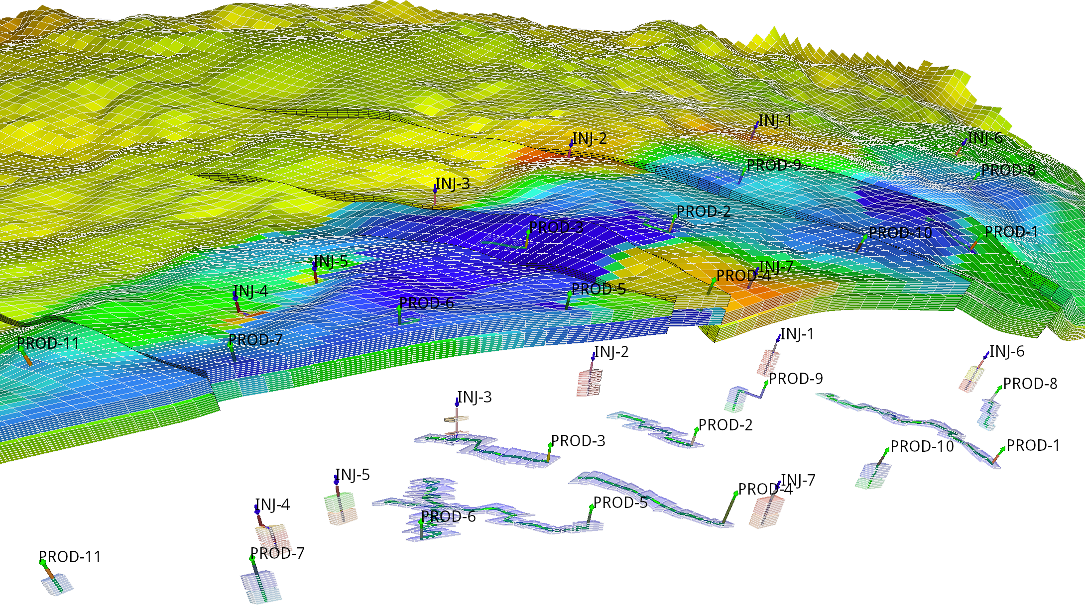
Figure 3: Case from the OLYMPUS Optimization Challenge [15]. Top: pressure at the end of the simulation time. Bottom: wells and the cells they are connected to.

2.2.1 Standard well model

For the standard well model, a single set of primary variables is introduced for each well. For a three-phase black oil system, there are four primary variables: $Q_{t}$ is the weighted total flow rate, the weighted fractions of water $F_{w}$ and gas $F_{g}$ describe the fluid composition within the wellbore [13], and the fourth is the bottom-hole pressure $p_{bhp}$, i.e., the pressure in the wellbore at the datum depth. The following equations relate the primary variables to the flow rates:

$$Q_{t} =\sum_{\alpha\in\{o,g,w\}}g_{\alpha}Q_{\alpha},\quad F_{w}=\frac{g_{w}Q_{w}}{Q_{t}},\quad F_{g}=\frac{g_{g}Q_{g}}{Q_{t}}$$ (17)

Here, $Q_{\alpha}$ is the flow rate of component $\alpha$ under surface conditions and $g_{\alpha}$ is a weighting factor. For gas, this factor is typically chosen to be a small value like $0.01$ to avoid gas fractions close to unity [13].

Volumetric inflow rates at reservoir conditions are calculated as

$$q_{\alpha,j}^{r}=T_{w,j}M_{\alpha,j}[p_{j}-(p_{bhp,w}+h_{w,j})],$$ (18)

where $q_{\alpha,j}^{r}$ is the flow rate of phase $\alpha$ through connection $j$. The other symbols are described in A.3. The rate is negative for flow from wellbore to reservoir, and positive for flow into the opposite direction. The pressure differences $h_{w,j}$ between connection $j$ and the datum point are computed explicitly based on the fluid composition in the wellbore at the start of the timestep.

To keep the system closed, we introduce conservation equations for each component,

$$R_{\alpha,w}=\frac{A_{\alpha,w}-A_{\alpha,w}^{0}}{\Delta t}+Q_{\alpha}-\sum_{j\in C(w)}q_{\alpha,j}=0,$$ (19)

that are solved in a fully implicit and coupled way with the black-oil equations (7). Here, $C(w)$ is the set of connections of the well $w$, $q_{\alpha,j}$ is the flow rate of phase $\alpha$ through connection $j$ under surface condition, which can be calculated from $q_{\alpha,j}^{r}$ defined in (18); the relation is similar to the one between component and mass fluxes (2). The storage term $A_{\alpha,w}$ describes the amount of component $\alpha$ in the wellbore (small volume), and it is introduced for better stability of the well solution.

In addition, we need equations that model how the wells are controlled. The well control for a well controlled by a prescribed bhp target reads

$$R_{c,w}=p_{bhp,w}-p_{bhp,w}^{target}=0,$$ (20)

whereas for a rate-controlled well we have

$$R_{c,w}=Q_{\alpha}-Q_{\alpha}^{target}=0.$$ (21)

where $Q_{\alpha}^{target}$ is the desired surface-volume rate of the controlled component $\alpha$, typically oil rate for a production well.

Under some conditions, fluids from the reservoir formation can enter the wellbore through some connections and get reinjected into the formation through other connections of the same well. This phenomenon is called cross-flow, and is modeled by the standard well model. Since the model assumes that the fluid composition is uniform throughout the wellbore (given by $F_{g}$ and $F_{w}$), the same composition will be injected through all injecting connections. When this is not accurate enough, a multi-segment well model can be used.

2.2.2 Multi-segment well model

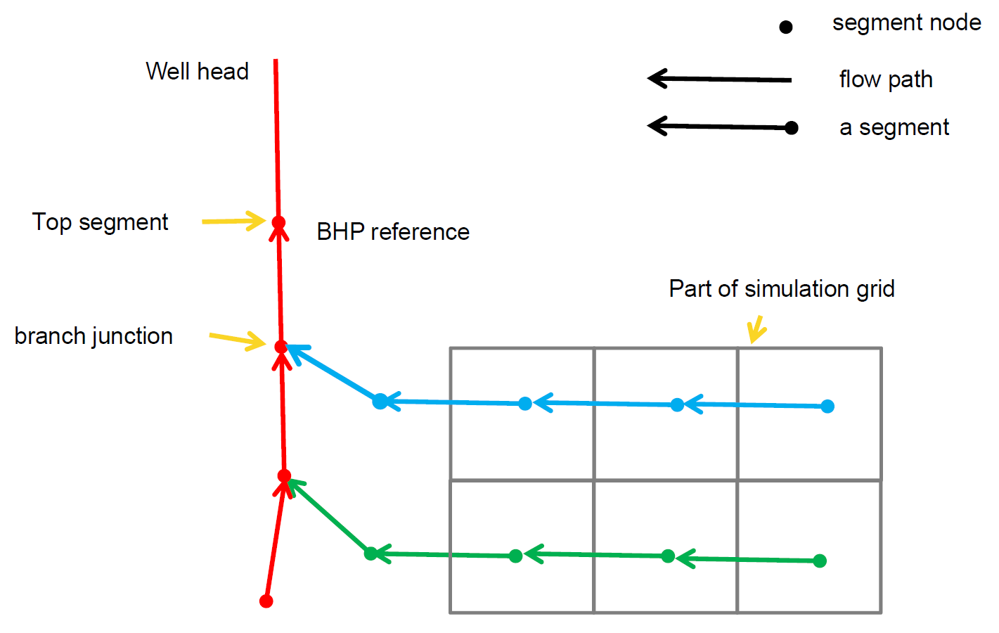
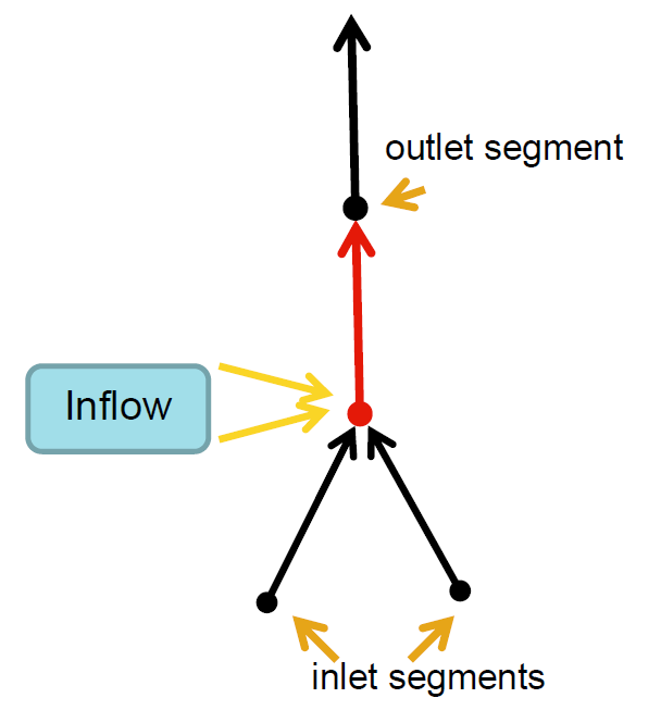
Figure 4: A illustration of the multi-segment well and the segment structure.

So-called multi-segment well models [14] were introduced to simulate more advanced wells, such as multilateral wells, horizontal wells, and inflow control devices. With a multi-segment model, the wellbore is divided into an arbitrary number of segments (Figure 4). Including more segments can give a more accurate simulation, at the cost of higher computational cost. Each segment consists of two parts: a segment node and a flow path to the neighboring segment in the direction towards the well head, defined as the outlet segment (Figure 4). Most segments also have inlet segment neighbors in the direction away from the well head. In the well shown in Figure 4, there are three branches, including one main branch (in red color) and two lateral branches (in green and blue colors). For multilateral wells, a segment node must be placed at the branch junction. Segments at branch junction points have additional inlet segments and segments at the end of branches do not have inlet segments. The top segment of each well does not have an outlet segment. The pressure at this segment is the bottom-hole pressure of the well, whereas the component rates equal the component rates for the well as a whole.

Each segment has the node pressure $p$ as a primary variable in addition to the primary variables $Q_{t}$, $F_{w}$, and $F_{g}$ introduced for the standard well model (see (17)). Likewise, the component equations (19) are extended to include additional terms $Q_{\alpha,i}$ that represent the flow rate from the inlet segments $I(n)$ of segment $n$ as well as the inflow from the reservoir through the segment’s connections $C(n)$.

$$R_{\alpha,n}=\frac{A_{\alpha,n}-A_{\alpha,n}^{0}}{\Delta t}-\sum_{i\in I(n)}Q_{\alpha,i}-\sum_{j\in C(n)}q_{\alpha,j}+Q_{\alpha,n}=0.$$ (22)

Each segment can thus receive inflow from more than one connection or no connection through the segment node, whereas each connection can only contribute to one segment. In the standard well model, the connection is located at the centroid of the grid block. In the multi-segment well model, the connection and segment node can be located any place in the grid block. The inflow calculation of the connection in the multi-segment well model is as follows:

$$q_{\alpha,j}^{r}=T_{w,j}M_{\alpha,j}(p_{j}+H_{cj}-p_{n}-H_{nc}).$$ (23)

Here, $p_{j}$ is the pressure at the cell center of the grid block that contains connection $j$; $H_{cj}$ is the hydrostatic pressure difference between the cell center and the connection; $p_{n}$ is the pressure of segment $n$; and $H_{nc}$ is the hydrostatic pressure difference between the connection and the segment (Figure 5).

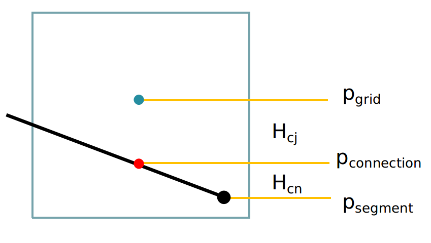
Figure 5: Hydrostatic pressure drops used in the multi-segment well model.

The last equation for each segment describes the pressure relationships between the segment $n$ and its outlet segment $m$:

$$R_{p,n}=p_{n}-p_{m}-H_{h}-H_{f}-H_{a}=0.$$ (24)

Here, the $H$ terms represent the hydrostatic, frictional, and acceleration pressure drops between the segments.

The top segment does not have a outlet segment, and hence the pressure equation is replaced by a well control equation, which is the same as for the standard well model, (20) or (21).

As with the standard well model, the well equations are solved with the reservoir mass conservation equations in a coupled, fully implicit way. The well equations are added to the global system as shown in Figure 6 using a Schur complement approach:

$$(A-\sum_{w}C_{w}D_{w}^{-1}B_{w})\,x_{r} =R_{r}-\sum_{w}C_{w}D_{w}^{-1}\,R_{w},$$ (25)

$$x_{w} =D_{w}^{-1}(R_{w}-B_{w}\,x_{r}).$$ (26)

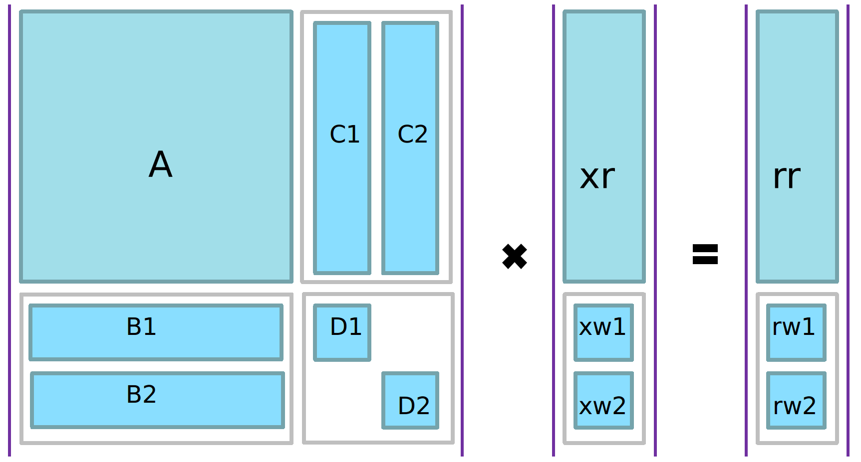
Figure 6: Partition of the matrix system for a case with two wells. Here, $A$ contains the reservoir flow equations, $D_{1}$ and $D_{2}$ contain the linearized well equations for each of the two wells, whereas the $B$ and $C$ matrices are coupling entries between the reservoir and well models.

2.3 Solution strategy

Altogether, the reservoir and well equations described thus far define a large system of (fully implicit) nonlinear equations, which we can write on compact residual form as $R(y)=0$, where $y$ is the vector of primary variables. This system is solved using a Newton–Raphson type method. Let $y_{n}=(p_{o},s_{w},x)$ be the primary variables after $n$ Newton iterations. Given an initial state $y_{0}$, the solution of $R(y)=0$ can be found by iteratively solving

$$J(y_{n})(y_{n+1}-y_{n})=-R(y_{n})$$ (27)

until $R(y_{n})$ is less then some prescribed tolerance. Creating the Jacobian matrix $J(y_{n})$ and solving this linearized problem is the core computational task of the simulator, and its performance depends largely on how this part of the code is programmed. The linearization and the solution procedure for (27) is explained in detail in the following subsections, but first some words about convergence of the nonlinear solver.

Because the solution at the end of the previous time step is used as initial guess, the Newton–Raphson is expected to converge rapidly if a sufficiently small time step is used. For large time steps and/or large changes in the solution, typically caused by changing well controls, the Newton–Raphson method may converge poorly or not at all. One simple way of improving the convergence is to restrict the change allowed per iteration and prevent the solution from jumping far across the boundary between saturated and undersaturated states in a single iteration. This so-called Appleyard chop technique [16] is implemented in OPM Flow, and is often sufficient for the method to converge. Still, time steps may need to be cut to make the solver converge for some difficult cases.

Note also that since the third primary variable $x$ may change interpretation from one iteration to the next, we are not strictly using the Newton–Raphson method as such, but a close relative. Changing primary variable may disturb the convergence, and we therefore add a small threshold to the variable-switching logic in (14) to prevent oscillation between states. Lack of smoothness of the residuals can also come from other sources. For example, the functions for relative permeability and capillary pressure can be almost discontinuous in some cases, they can also have hysteretic behaviour.

The third point that affects the convergence of the nonlinear solver is the accuracy of the linear solvers. Solving the linear system to a loose accuracy may lead to poor convergence of the nonlinear solver. The tuning of the time-stepping procedure, and the tolerance used in the linear and nonlinear solvers are highly related, and optimal choices are case- and problem-dependent.

From the user side, there are several command-line options that can be used to control the solver. In particular, --tolerance-mb controls the mass balance error as a reservoir-average saturation error, and --tolerance-cnv controls the maximal local residual error. For more information about runtime options and other aspects of running OPM Flow, see Section 2.2 of the OPM Flow manual [10]. Running OPM Flow with the option --help will print a list of available parameters.

2.3.1 Solving the system of linear equations

Depending on fluid properties and other reservoir-specific parameters, the system of equations (7) could exhibit elliptic or degenerate parabolic behavior or could even be hyperbolic for specific setups. Therefore, solving the linearized system (27) stemming from these equations is challenging, since it is likely non-symmetric and ill-conditioned. Instead of solving equation (27) directly, the solution is approximated by an iterative linear solver. Two variants are available, a stabilized Bi-conjugate Gradient method (BiCG-stab) and a restarted Generalized Minimal Residual (GMRes) solver. By default, BiCG-stab is used. In addition, several options are available for preconditioning of the linear system, the default choice being the incomplete lower triangular–upper triangular factorization with level of fill in $0$ (ILU0). More sophisticated choices are based on an algebraic multigrid (AMG) method for preconditioning, such as a recently added Constraint Pressure Residual (CPR) preconditioner (originally introduced in [17]) using the approach of [18].

Implementation of the AMG and the CPR preconditioner is further discussed in Section 2.5 and the solver itself in [19]. The OPM Flow manual [10] gives an overview of parameters for choosing solvers and preconditioners, as well as other related parameters. The solvers and preconditioners are implemented in the Dune module dune-istl and described in [20, 21]. In the current version, OPM Flow assembles the Jacobian matrix into the block compressed row storage (BCRSMatrix) data structures provided by dune-istl. Each matrix entry is of the type FieldMatrix, which is a dense matrix with fixed row and column length provided by dune-common. Blocked matrix storage enables better performance on modern CPUs compared to the standard approach that stores each matrix entry separately. Likewise, the unknown $\Delta y$ and the right hand side $-R(y_{n})$ are stored in a BlockVector from the dune-istl package.

The interface between OPM Flow and linear solver packages has been designed in a flexible way so that besides dune-istl other linear algebra packages could be used. For example, an experimental implementation using the PETSc library [22] has been successfully tested. This is, however, not yet part of the main branch of the source code.

2.4 Automatic differentiation in OPM Flow

The coefficients of the linearized systems required by the nonlinear Newton solver (e.g., $J(y_{n})$ in equation (27)) have traditionally been computed by evaluating closed-form expressions obtained by differentiating the discretized flow equations analytically. Differentiating these flow equations manually and programming the resulting formulas is both time-consuming and error-prone. The problem is particularly pronounced when extending an existing simulator with new functional relationships. If a quantity is set to depend on a different or new (primary) variable, the changes in derivatives will propagate through the chain rule to the Jacobians of all quantities that depend on the modified quantity. Thus, even very simple extensions in functional dependencies may cause large modifications throughout the simulator code.

Automatic differentiation (AD) is a way to mitigate this problem; see for example [23] or [8] for an introduction. There are many examples of AD tools used for scientific computing, such as Sacado, ADOL-C [24] or ADETL; the latter used for the AD-GPRS reservoir simulator.

The AD mechanism implemented in OPM works by treating each quantity in the program not as just a single value, but as a value paired with values for the “relevant” partial derivatives. Whenever the value of a new quantity is computed, a combination of the chain rule and standard differentiation rules for elementary unary and binary operations is used to compute the correct value of all the corresponding partial derivatives. This is called the forward approach to AD, in contrast to backward AD, which stores the adjoints of each quantity.

The drawback is that an AD library must be learned, or developed from scratch if no existing library matches the needs of the application at hand. In OPM’s case, we decided to develop a library from scratch, since no existing packages provided the desired flexibility and performance, and we also could not find a suitable freely licensed package. Further, experience from developing a similar library in MRST [5] made the implementation effort of OPM’s AD library relatively small.

The cost of AD for the user can be lower performance compared to a well-tuned hand-written implementation. We have made numerous improvements to our automatic differentiation implementation to reduce this overhead, but it is clear that by investing sufficient effort into a hand-written code, one can possibly get better performance. Writing such optimal Jacobian code for arbitrary extensions is not a trivial task, and due to the increased chance for errors is not guaranteed to give any speed-up at all.

2.4.1 General approach

The OPM implementation of AD introduces a class that mimics the behaviour of the built-in floating point types of C++ (double and float) as closely as possible. The AD object contains a value and a fixed number of derivatives and defines all basic arithmetic operators as well as common mathematical functions. Also, to allow easy comparisons with code that uses standard floating-point objects, all functions that work on AD-objects can also be used with objects of built-in floating-point types. In OPM an implementation class called Evaluation is provided for this purpose:

⬇

1 // ValueT is typically double or float

2 template <class ValueT, int numDerivs>

3 class Evaluation;

This class overloads all arithmetic operators so that objects of type Evaluation can be used in the same way as plain double or float types. An example code snippet for the implementation of the multiplication operator looks as follows:

C++ code

⬇

1Evaluation& operator*=(const Evaluation& other)

2{

3 // The values are multiplied, whereas the derivatives

4 // follow the product rule, i.e., (u*v)’ = (v’u + u’v).

5 const ValueType u = this->value();

6 const ValueType v = other.value();

7 // Value, usually position 0

8 data_[valuepos_] *= v ;

9 // Derivatives usually start at position 1

10 for (int i = dstart_; i < dend_; ++i) {

11 data_[i] = data_[i] * v + other.data_[i] * u;

12 }

13 return *this;

14}

For improved performance the implementation of the Evaluation class is specialized for values with up to $12$ partial derivatives, whereas a default implementation based on for loops is used for higher numbers of derivatives. The opm-material module provides a python script implementing a simple code generation algorithm for the specialized Evaluation classes for any number, if necessary. Typical three-phase black-oil equations use three partial derivatives, corresponding to the number of primary variables per cell.

2.4.2 Application-specific localization

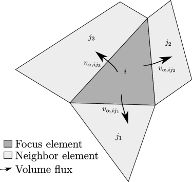
Figure 7: Localized linearization of element $i$ and its neighbors $j_{\left<\cdot\right>}$. Equations (7) are evaluated locally with derivatives of the primary variables of element $i$.

For performance reasons, the implementation of automatic differentiation in OPM only supports carrying a fixed number of derivatives, which needs to be specified at compile-time. Yet, the number of unknowns for the discretized conservation equations (7) is only known at run-time because it depends on the number of grid cells.

This problem is solved using a localized linearization scheme as illustrated by Figure 7: The residuals of the mass conservation equations are computed for a single element, which is called the focus element. In addition to the values of the residuals of the focus element, the partial derivatives of the residuals of all elements in the local neighbourhood are calculated with regard to the fixed number of primary variables of the focus element. For more details on this approach, confer [25].

The two-point flux-approximation (TPFA) scheme used ensures that the residuals of any cell only depend on the variables of the cell itself and its immediate neighbours, which lets the localized linearization scheme be applied.

Once the local residual vector and its dense Jacobian matrix have been computed, they are transferred to a variable-sized vector for the residual and a variable-sized sparse matrix for its Jacobian matrix representing the linearized system of equations for the whole spatial domain. This vector and the matrix are subsequently passed to the linear solver.

2.5 Parallelization

Parallelization of OPM Flow follows a hybrid approach with a combination of multi-threading and MPI. The assembly of the Jacobian matrix is multi-threaded through OpenMP, and controllable through the OpenMP environment variables. The assembly part is less dependent on memory bandwidth, and this enables us to exploit more CPUs on a multicore machine than the scaling possible for the linear solve part. In particular, it allows for improved performance on CPUs with hyper-threading. Writing binary results to file is also threaded to insulate the reservoir simulation from slow disk systems, as further commented on in Section 2.6. The CpGrid class implementing stratigraphic grids is based on the Dune grid interface and OPM Flow therefore naturally inherits the MPI parallel interface of the Dune modules dune-grid and dune-istl (see [1, 26, 21]). This keeps the implementation effort as small as possible. Our main goal is to reuse sequential algorithms whenever possible and only introduce parallelism specific code where absolutely necessary. In particular, the discretization, and algorithms for adaptive time stepping and the Newton–Raphson nonlinear solver are the same for sequential and parallel runs. For the latter, only the convergence criterion will be switched to a parallel one as it needs some global communication.

Standardized parallel file formats for oil reservoir data are currently lacking and the ECLIPSE file format is inherently sequential in nature (see Section 2.6). At the beginning of a simulation, a process therefore needs to read the complete input file and set up a grid for the entire domain. This is a potential bottleneck for scalability to large number of cores, which has not yet been reached. Using the entire grid read initially, the transmissibilities representing cell–cell connections are computed. A high value means that a change of pressure or saturation in a cell will influence the properties of the neighboring cell strongly. Therefore, the current domain decomposition in OPM Flow is based on keeping cells connected through high transmissibilities on the same process when partitioning. This is done to ease the coarsening phase of the algebraic multigrid solver and improve convergence of other linear solvers. The implementation currently does not allow one well to be distributed across multiple subdomains.

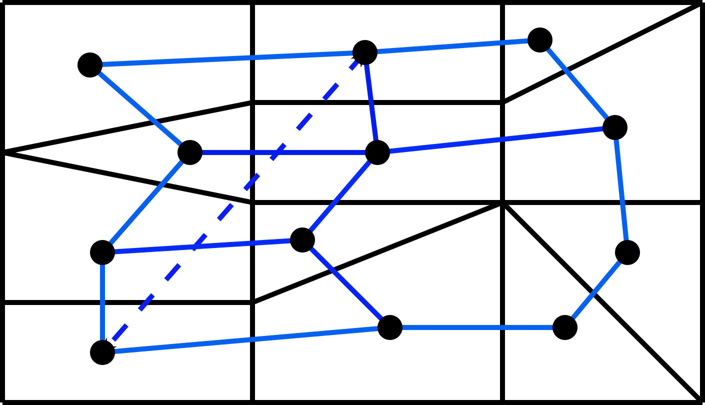
Figure 8: Graph of a grid with one well, where the black dots are the vertices associated with cells in the grid and the blue lines the edges associated with the cell faces. The dashed blue line is an edge introduced by a well connecting two non-neighboring cells.

At the start of the simulation, the global grid is partitioned using the graph partitioning software Zoltan [27, 28] on the grid graph defined with cells as vertices and edges graph either representing a face between two cells or a connection between two cells via a well. Figure 8 shows a conceptual illustration. An edge associated with a cell face is assigned the value of the transmissibility, scaled by $10^{18}$, whereas any edge associated with a well connection gets the maximum weight available to ensure that all cells connected by a well end up in the same subdomain. This will give partitions in which domain boundaries are at faces having low transmissibility. In a post-processing step after the initial load balancing, we ensure that all cells connected by a well are really contained in one subdomain since our edge weights are merely a strong suggestion to the load balancer. As a result, the calculation of the well model can be done sequentially on the process that stores the well without additional communication.

The flux calculation, which is a central part of any cell-centered finite-volume scheme, needs to access information from neighboring cells. OPM Flow therefore not only stores the grid cells assigned to one process, but also a halo layer of so-called ghost cells at the process boundary. During the simulation, the values attached to these ghost cell are updated using point-to-point communication. Figure 9(a) illustrates the local grid stored on one process.

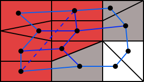
(a) Interior and ghost layer

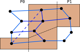
(b) Communication

Figure 9: (a) Interior (red) and ghost (grey) cells stored on a process, and (b) grid cells involved in communication.

This decomposition is used to set up a distributed view of the CpGrid class. It implements the parallel Dune grid interface ([1, 26]) allowing values attached to interior cells to be easily communicated to other processes, where these cells belong to the ghost layer. For the small example in Figure 9(b), only the brown cells will be involved in the communication.

As a result, the sequential discretization algorithms can be reused almost unchanged, since all necessary data (neighboring and wells) is available on one process and only one communication step during each linearization step of the nonlinear solver is needed to update the ghost layer.

The iterative solvers in dune-istl are parallelization agnostic and can be turned into parallel ones by simply using parallel versions of the preconditioner, scalar product, and linear operator. All preconditioners, except AMG, apply the sequential operator on the degrees of freedom attached to the interior cells only and update the rest using one step of interior-ghost communication. When used in AMG as smoothers, these parallel preconditioners are called hybrid smoothers (see [29]). This approach works very well in the AMG solver provided by dune-istl [19], as it uses data agglomeration onto fewer processes whenever the number of unknowns per process dops below a prescribed threshold. Thus on coarser levels fewer processes are involved in the computation until on the coarsest level only one process computes and a direct coarse solver is used. This remedies the missing smoothing across the processor partition boundaries on the finer levels and keeps the ratio between time used for computation between communication steps and time needed for communication high. In addition, a block ILU0 (one block for each process) or a CPR preconditioner is provided. Both the existing parallel scalar product and linear operator from dune-istl are reused without modifications.

2.6 I/O in OPM Flow

To be industrially relevant, OPM Flow must read and write files in standard formats well known to the industry. OPM Flow implements support for the input format used by the ECLIPSE simulator from Schlumberger and also writes output files compatible with the output from said simulator, because this is the dominant file formats supported by most pre- and post-processing tools.

2.6.1 Reading input files

The input for a simulation case consists of many separate data items. The computational grid, petrophysical properties, fluid properties, and well scheduling and behavior must all be specified, along with other options controlling for example output.

It is common for commercial simulators to do this in the form of an input file set, often called a deck (named for the decks of punched cards used in the early age of simulation). An input deck consists of many keywords that set properties or trigger functionality in the simulator, and may be distributed across several files (using an INCLUDE keyword). The deck is organized into sections dealing with separate parts, and is similar to a programming language that manipulates the reservoir simulator like a state machine. The sections are:
RUNSPEC Dimensions, phases present. GRID Grid topology and geometry, faults, petrophysical properties. EDIT Modifying inputs specified in the GRID section, multipliers. PROPS Fluid properties. REGIONS Define regions for properties and output. SOLUTION Initial solution. SUMMARY Choose variables for time-series output. SCHEDULE Parameters and controls for wells and well groups, time stepping.

The input format is well documented in the OPM Flow manual [10]. The sections are described in Chapter 3.4 of the manual, and each supported keyword is described in the following chapters. The list of supported keywords is extensive, and the parsing performed in OPM Flow has been tested on a selection of different input decks from industry. For obvious reasons, OPM Flow does not yet support all keywords and features available in the ECLIPSE simulator. Still, OPM Flow is fast reaching a point where the functionality available covers the most common use cases, and is wide enough that it can be feasible to modify unsupported cases to adapt their reservoir description to what is currently supported. We therefore believe the current parsing framework is sufficient to make OPM Flow an attractive alternative in the industry.

Parsing in OPM Flow is a two-stage process. In the first stage, basic string parsing is performed, comments are stripped, included files are read in, default values and multipliers are resolved, and numerical items are converted to the correct type. This produces an instance of class Opm::Deck, which is essentially a container of Opm::DeckKeyword objects. The second stage in the parsing process consists of creating an instance of type Opm::EclipseState, which is an object at a much higher semantic level, in which the interaction between keywords has been taken into account, e.g., all the EDIT section modifiers have been applied to produce consistent geological input fields and the various well-related keywords from the SCHEDULE section have been assembled into well objects.

The keywords recognized by OPM Flow are specified with a simple JSON schema. A new keyword can be supported by adding a JSON specification and registering it with the build system, then OPM Flow will be able to parse the new keyword and create Opm::DeckKeyword instances to represent it. Taking a new keyword into account in the Opm::EclipseState class requires changes to the code depending on the semantics of the new keyword. To complete the addition of a new feature, the numerical code can then be extended to use the new information available from the Opm::EclipseState object.

2.6.2 Writing output files

OPM Flow can output a range of different file types. Summary files contain time-series for well or reservoir data. Restart files, along with INIT and EGRID files, can be used for restarting a simulation from a report step or checkpoint, as well as for visualization of the reservoir and the solution variables. RFT files are used by engineers to get more information about reservoir behavior.

The files are ECLIPSE-compatible in the sense that they are correctly rendered in independent third-party viewers like Petrel, S3Graf, and RMS, in addition to OPM ResInsight. These binary output files are also compatible to the point that Schlumberger’s simulator ECLIPSE can restart a simulation from these files.

The input keywords RPTRST, RPTSOL, and RPTSCHED are used to configure which properties should be written to the restart files, and also for which report steps output should be enabled, most of this output configuration is supported in OPM Flow.

The SUMMARY section is used to configure which result vectors should be added to the summary output. OPM Flow will use the configuration inferred from this section when creating summary output. The list of available summary vectors is extensive and OPM Flow does not support them all, but a wide range of field, group, well, region, and block vectors are supported. In addition, OPM Flow has its own unique PRT file, which has a report formatted just like ECLIPSE for compatibility. However, everything else in the PRT file is unique for OPM Flow. The same goes for the terminal output, which is not the same as ECLIPSE. The ambition is to make output more useful for the end user.

VTK-format output files for result fields can also be written for visualization with, e.g., Paraview. This feature can be activated with a command-line option, see the manual [10] for this and other output-related options.

2.6.3 Parallel file I/O

The ECLIPSE file format is inherently sequential, but since this file format is a de-facto standard in the industry, the parallel simulation program also needs to handle the format. Whereas initial reading of the deck is less performance critical, since it is only done once, the reoccurring writing of simulation data during the simulation poses a potential performance bottleneck. To absorb the penalties imposed by slow file systems, such as network file systems, the actual output is queued in a separate output thread that no longer needs to by synchronized with the simulation. To cater to the sequential file format at hand, a dedicated I/O rank collects all data from all processes and then the sequential output routines can be used as before. Again, this is a potential show stopper for scaling to large number of cores; this has not been an issue yet, but may need to be addressed in future releases of the software. To avoid performances penalties, the communication between the I/O rank and all other ranks is done asynchronously, such that each simulation core only places an MPI_Isend and continues with simulation, whereas the I/O rank only places MPI_Irecv in combination with MPI_Iprobe and MPI_Waitall.

2.7 Extended models

Whereas the family of black-oil models presented thus far is sufficient for many real-world cases, it lacks essential features for describing chemically enhanced oil recovery. This section briefly outlines two extended models implemented in OPM Flow, a solvent model and a polymer model, that add one or a few extra components and model their effect on the fluid flow.

2.7.1 Solvent

Miscible gas injection is a common EOR technique. The injected gas mixes with the hydrocarbons and enhances the sweep efficiency by mobilizing the residual oil in the reservoir. An important application for the solvent module in OPM is to explore the combined goal of CO₂ storage with EOR. The CO₂ is miscible with oil at pressures above a certain threshold, and injecting CO₂ is thus a commonly used approach to enhanced recovery.

The solvent module extends the black-oil model with a fourth component representing the injected gas. In addition to the extra conservation equation required for the solvent, the solvent modifies the relative permeability, the capillary pressure, the residual saturations, the viscosity, and the density of the hydrocarbons. The modeling strategy we use is to compute the properties for the fully miscible and the immiscible case and interpolate between these limits using a miscibility function $M$ depending on pressure and solvent saturation.

Large contrasts in viscosity and density between the injected gas and the oil lead to fingering effects. Resolving individual fingers requires very fine grid resolution and is not feasible for field-scale simulations. The Todd–Longstaff model [30] introduces an empirical parameter $\omega$ to formulate effective parameters that take into account the effect of fingers on the fine-scale dispersion between the miscible components to overcome this obstacle. The solvent module in OPM follows the implementation suggested in [30, 31], the most important details are included here.

The conservation equation for the solvent component, $s$, is

$$\frac{\partial}{\partial t}\left(\phi_{\rm ref}A_{s}\right)+\nabla\cdot{\bf u}_{s}+q_{s} =0,$$ (28)

where the accumulation term and the flux are given by

$$A_{s}=m_{\phi}b_{s}s_{s},\qquad{\bf u}_{s}=-b_{s}\lambda_{s}{\bf K}(\nabla p_{g}-\rho_{s}{\bf g}).$$ (29)

In addition, the solvent saturation is added to Equation (4), giving:

$$s_{w}+s_{o}+s_{g}+s_{s}=1.$$ (30)

The relative permeability of the solvent and the gas component is given as a fraction of the total (gas + solvent) relative permeability:

$$k_{r,s}=\frac{s_{s}}{s_{g}+s_{s}}k_{r,gt},\qquad k_{r,g}=\frac{s_{g}}{s_{g}+s_{s}}k_{r,gt}.$$ (31)

One can change the gas and solvent fractions multiplying $k_{r,gt}$ with simple functions of the same fractions to allow a more flexible formulation. The total relative permeability is given as an interpolation between the fully miscible relative permeability and the immiscible one:

$$k_{r,gt}=M\frac{s_{g}+s_{s}}{s_{g}+s_{s}+s_{o}}k_{r,n}(s_{n})+(1-M)k_{r,g}(s_{g}+s_{s}),$$ (32)

$$k_{r,o}=M\frac{s_{o}}{s_{g}+s_{s}+s_{o}}k_{r,n}(s_{n})+(1-M)k_{r,o}(s_{w},s_{g}),$$ (33)

where $M$ is a user-defined parameter that varies from zero to one and may depend on both the solvent fraction and the oil pressure. Water-blocking effects are incorporated in the model by further scaling the normalized saturations by effective mobile saturations that increase with increasing water saturation; see [31] for details.

The Todd–Longstaff model formulates the effective viscosities for solvent, gas, and oil as a product of the pure viscosities and the fully mixed viscosity

$$\mu_{{\rm eff},o}=\mu_{o}^{1-\omega}\mu_{m,os}^{\omega},\quad\mu_{{\rm eff},g}=\mu_{g}^{1-\omega}\mu_{m,gs}^{\omega},\quad\mu_{{\rm eff},s}=\mu_{s}^{1-\omega}\mu_{m,gos}^{\omega},$$ (34)

where the fully mixed viscosities are defined using standard $\tfrac{1}{4}$-power fluid mixing rule [30]. Pressure effects on the mixing are modeled by replacing the single parameter $\omega$ with an effective mixing parameter

$$\omega_{\rm eff}=\omega\omega_{p}.$$ (35)

where $\omega_{p}$ is a function of pressure [31, 32]. For effective density calculations confer [31]. The solvent model is used to simulate the SPE 5 benchmark in Section 3.3,

2.7.2 Polymer

Polymer flooding is another widely used EOR technique. The major mechanism of polymer flooding is to improve the sweep efficiency by increasing the viscosity of the drive fluid to improve the mobility ratio. The polymer model in OPM assumes that the polymer component is only transported within the water phase and only affects the properties of this phase. The model also includes the effects of dead pore space, polymer adsorption in the rock, and permeability reduction effect. Shear-thinning/thickening non-Newtonian fluid rheology is modelled by a logarithm look-up calculation method based on the water velocity or shear rate.

The polymer model is developed by adding the following polymer transport equation to the black-oil model

$$R_{p,i}=\frac{V_{i}}{\Delta t}(A_{p,i}-A_{p,i}^{0})+\sum_{j\in C(i)}F_{p,ij}+q_{w,i}c_{w,i}=0,$$ (36)

where

$$A_{p,i}=\phi_{{\rm ref},i}m_{\phi}b_{r}b_{w}s_{w}(1-s_{dpv})c+\rho_{r}C^{a}(1-\phi_{{\rm ref},i})$$ (37)

$$F_{p}=b_{w}v_{p}c$$ (38)

$$(b_{w}{v}_{p})_{ij}=\Bigl{(}\frac{m_{T}k_{r,w}}{\mu_{{\rm eff},p}R_{k}}\Bigr{)}_{U(w,ij)}T_{ij}\Delta H_{w,ij},$$ (39)

$$(b_{w}{v}_{w})_{ij}=\Bigl{(}\frac{m_{T}k_{r,w}}{\mu_{{\rm eff},w}R_{k}}\Bigr{)}_{U(w,ij)}T_{ij}\Delta H_{w,ij}.$$ (40)

Here, $c$ is polymer concentration, $b_{r}$ is rock expansion factor, $s_{dpv}$ is the dead pore space, $C^{a}$ is the polymer adsorption concentration, ${v}_{p}$ is polymer flux rate, and $\mu_{{\rm eff},p}$ is the effective polymer viscosity, which is a function of the polymer concentration $c$ and pressure of the water phase. The viscosity of water is changed as a result of dissolution of polymer, and we calculate the water flux rate based on effective water viscosity $\mu_{{\rm eff},w}$, which is also a function of polymer concentration. The polymer concentration $c_{w,i}$ used to calculate the polymer rate through well connections in grid block $i$ is set as the injection concentration for injectors, whereas $c_{w,i}=c_{i}\mu_{{\rm eff},w}/\mu_{{\rm eff},p}$ for producers, where $c_{i}$ is the polymer concentration in grid block $i$. The effective viscosities are calculated using the Todd–Longstaff mixing model [30] to handle sub-grid fingering effects, similar to the solvent model of Section 2.7.1.

3 Numerical examples and results

This section demonstrates OPM Flow through a series of numerical examples. Sections 3.1 to 3.3 report small synthetic cases exercising particular parts of the simulator’s fluid behavior. Section 3.4 reports a more realistic case to highlight the treatment of wells. The Norne case in Section 3.5 is a real field case and demonstrates that OPM Flow can be applied to complex industrial field cases. The polymer example in Section 3.6 shows some of the EOR capabilities of OPM Flow.

We conclude the section with some notes on performance. Complete input decks used for the examples are available from github.com/OPM, and can be run with default options.

3.1 SPE 1 benchmark

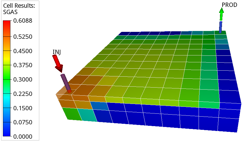
Figure 10: Gas saturation of the SPE 1 benchmark case after a period of gas injection. The z-axis has been exaggerated 20 times.

The Society of Petroleum Engineers (SPE) has run a series of comparative solutions projects with the aim of comparing and benchmarking different simulators or algorithms. The first such project (nicknamed SPE 1), was introduced for benchmarking three-dimensional black oil simulation [33]. Two examples were suggested, and here we use the second case to demonstrate OPM Flow. The grid consists of 10$\times$10$\times$3 cells covering a computational domain of 10 000 ft$\times$10 000 ft$\times$100 ft. The thickness of each layer is 20 ft, 30 ft, and 50 ft respectively. Two wells are located in two opposite corners. The first well injects gas from the top layer at a rate of 100 MMscf/day with a BHP limit of 9014 psia. The other well is set to produce oil from the bottom layer with a production target of 20 000 stb/day and BHP limit of 1 000 psia. The reservoir is initially undersaturated. The participants were asked to report the oil production over time and the gas-oil ratio (GOR) over time. Figure 10 shows a view of the case after a few years of injection, whereas Figure 11 verifies that there is excellent agreement in the well responses computed by OPM Flow and the commercial simulator ECLIPSE 100.

(a) Bottom hole pressure of the injector

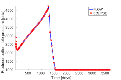
(b) Bottom hole pressure of the producer

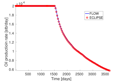
(c) Oil production rate of the producer

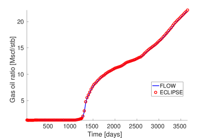
(d) Gas-oil ratio of the producer

Figure 11: Well responses computed for the SPE 1 benchmark, Case 2.

3.2 SPE 3 benchmark

The third comparative solution project [34] was introduced to study gas cycling of retrograde condensate reservoirs using compositional modeling. Based on the data initially provided as the second case in [34], we designed a benchmark test case for the OPM Flow simulator.

Black-oil properties are generated from compositional data using PVTsim Nova. The dimension of the grid is 9$\times$9$\times$4 with 293.3 ft $\times$ 293.3 ft cell sizes in the horizontal direction and the thickness of each layer being 30 ft, 30 ft, 50 ft and 50 ft, respectively. The horizontal permeability for each layer is 130 md, 40 md, 20 md, and 150 md respectively, whereas the vertical permeabilities are 13 md, 4 md, 2 md, and 15 md.

An injector is located in the corner (cell column (1,1)) and perforates the top two layers, whereas a producer perforates the bottom two layers of cell column (7,7). The simulation time is 14 years in total. The gas injection rate is 5700 Mscf/day for the first four years, and 3700 Mscf/day for the next five years. No gas is injected the last five years. The BHP limit is a constant 4000 psia. The production well operates with a constant gas production limit 5200 Mscf/day and a constant BHP limit of 500 psia. Figure 12 confirms good agreement for bottom-hole pressures and rates obtained by OPM Flow and ECLIPSE.

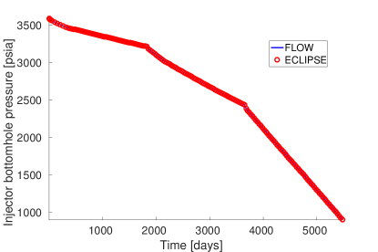
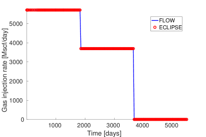
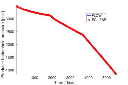
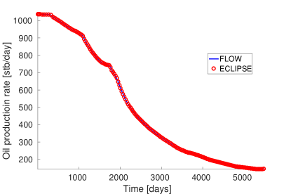
Figure 12: Bottom-hole pressures and well rates of the SPE 3 benchmark, Case 2.

3.3 SPE 5 benchmark

The fifth comparative solution project [35] is designed to compare four-component miscible simulators with fully compositional simulators for three different miscible gas injection scenarios. Herein, we compare the solvent simulator in OPM is compared with the solvent simulator in ECLIPSE for the three cases introduced in the SPE 5 paper. The same grid with dimension 7$\times$7$\times$3 and the same fluid properties are used for all the cases. A water-alternating-gas (WAG) injector is located in Cell (1,1,1). By changing the alternation sequence and rates of water and gas, different miscibility conditions are obtained in the three different scenarios. A producer located in Cell (7,7,7) is controlled by the same oil production rate in all three cases; see [35] for details, or confer the input deck given in opm-data.

Figure 13 shows that, except for some minor discrepancies in the gas production rate and the injector bottom-hole pressure, there is general agreement between the well responses computed by OPM Flow and those computed by the solvent module in ECLIPSE. A closer investigation reveals that the discrepancies are mainly caused by differences in how the density mixture of the Todd–Longstaff model is implemented. To the best of our knowledge, both simulators uses the same model, but the complexity of the model may lead to differences in the actual implementation.

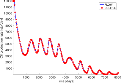
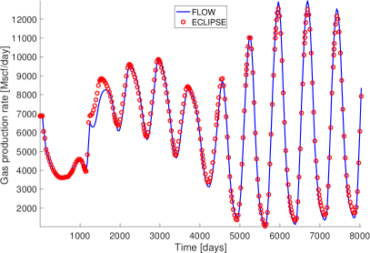
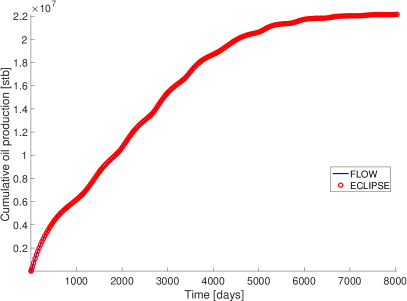
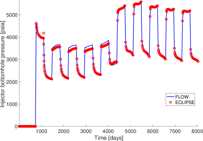
Figure 13: Oil production rate, gas production, and cumulative oil production of the producer, as well as bottom-hole pressure of the injector for the SPE 5 benchmark, Case 1.

3.4 SPE 9 benchmark

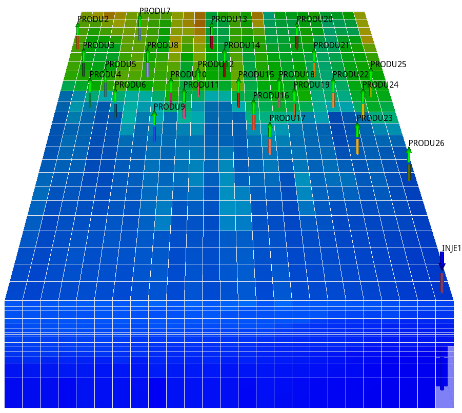
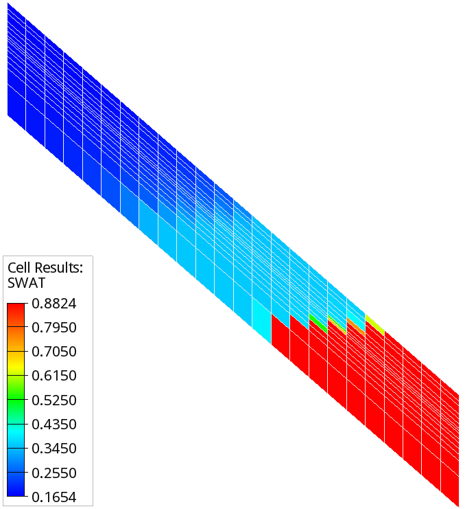
Figure 14: Left: frontal view of the SPE 9 benchmark case showing free gas saturation at the end of the simulation, and all wells. Right: side view showing initial water saturation. The z-axis is exaggerated 5 times in both plots.

The ninth comparative solution project [36] is designed to re-examine black-oil simulation. The model includes a rectilinear grid with 9 000 grid cells and the dimension is 24$\times$25$\times$15 (Figure 14). Originally, the grid was provided in conventional rectangular coordinates. In opm-data, we provide data sets also in the corner-point grid format. Cell (1, 1, 1) is at a depth of 9 000 feet, and the remaining part of the grid is dipping in the $x$-direction with an angle of 10 degrees. The model has a layered porosity structure and highly heterogeneous permeability field. The well pattern consists of 25 rate-controlled producers and one injector in the corner of the grid.

The total simulation time is 900 days. The injector is controlled by water injection rate with target rate 500 stb/day and BHP limit 4 000 psia. The producers are under oil rate control with BHP limit 1 000 psia. The production rate target is 1 500 stb/day for all the producers, except between 300 and 360 days, when the rate target is temporarily lowered to 100 stb/day.

This benchmark exercises in particular the well model of the simulator and its interaction with the reservoir. It also has nontrivial phase behaviour, as initially there is no free gas in the reservoir, but as pressure is reduced below the bubble point, free gas appears near the top, as can be seen in Figure 14. Figure 15 shows that the well curves computed by OPM Flow and ECLIPSE are in excellent agreement.

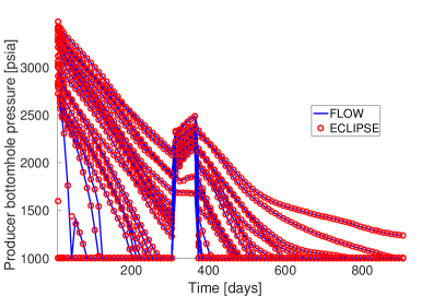
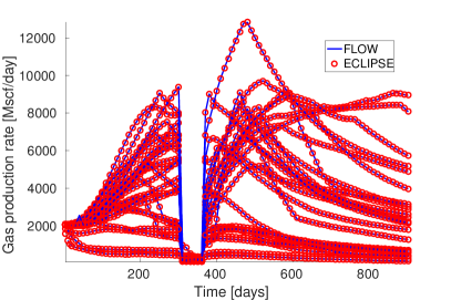
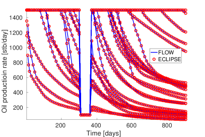
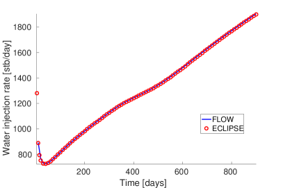
Figure 15: Bottom hole pressures, gas production rates, and oil production rates for all producers in the SPE 9 benchmark. Water rate are also reported for the injector.

3.5 Norne

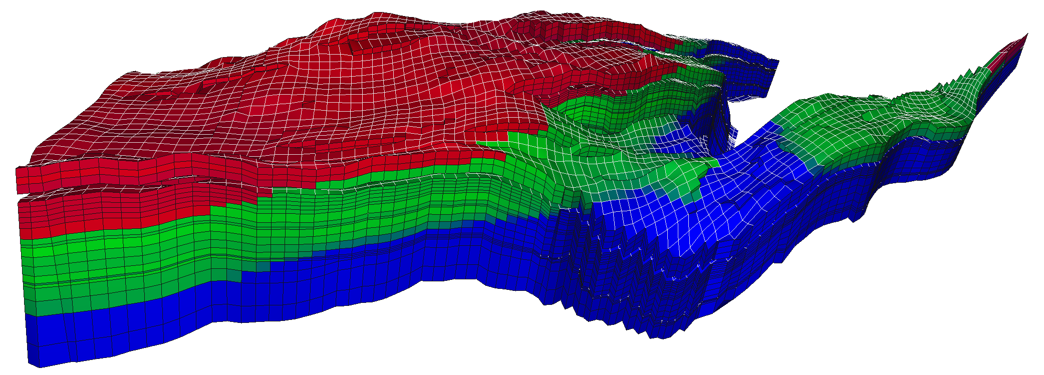
Figure 16: Grid for the Norne field case, with initial fluid distribution. Red is gas, green is oil, and blue is water.

Norne is a Norwegian Sea oilfield that has been in production since 1997. The operators of the field have chosen to share data, making it the only real field simulation case that was openly available until 2018, when the Volve field data were also made open. The Norne field was initially operated using alternating water and gas injection, and in total 36 wells have been opened, not all being active at the same time. The simulation model uses a corner-point grid with sloping pillars and several faults, so the grid has many non-logical-Cartesian connections and is therefore completely unstructured and challenging to process.

The Norne field model includes features such as hysteresis, end-point scaling, oil vaporization control, and multiple saturations regions. For a full description or to test the model, confer to github.com/OPM. Figure 17 shows that there also in this case is excellent match between OPM Flow and ECLIPSE, despite the complexity of the model.

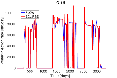
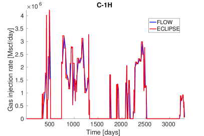
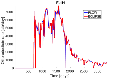
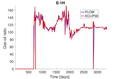
Figure 17: Well responses for injector C-1H and producer E-1H of the Norne field.

3.6 Polymer injection enhanced oil recovery (EOR) example

To demonstrate the use of the polymer functionality of OPM, we consider a simple 3D example taken from [37]. The grid consists of 2 778 active cells and is generated with MRST [4]. The reservoir has physical extent of 1 000m $\times$ 675m $\times$ 212m and contains one injector and two producers (Figure 18). The injector is under rate control with target rate 2 500 m³/day and bottom-hole pressure limit 290 bar. The producers are under bottom-hole pressure control with a bottom-hole pressure target of 230 bar.

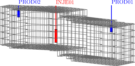
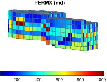
Figure 18: Computing grid and horizontal permeability of the polymer example.

The flooding process begins with a 560-day pure water injection, then a 400-day polymer injection with concentration 1.0 kg/m³, followed by a 1 530-day pure water injection. Four different kinds of configurations compared. In the first, no polymer is injected. The second includes polymer, but does not account for any shear effect. The third models shear-thinning effects, whereas the fourth includes shear-thickening effects.

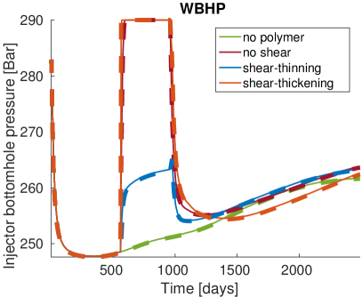
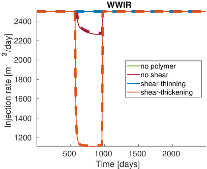
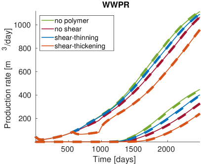
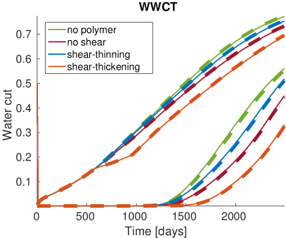
Figure 19: Well responses for the polymer flooding case. The top plots show bottom-hole pressure (left) and water rate (right) for the injector. The bottom plots show water rates and water cuts for the two producers. Results from OPM Flow are shown with thin lines, ECLIPSE results with thick dashed lines.

Figure 19 reports well responses for all four configurations. The bottom-hole pressure (bhp) of the injector increases when the polymer injection process starts. When no-shear effect is involved, the bhp reaches the limit, and the injector switches to bhp control mode, which causes decreased injection rate. This is a natural consequence of reduced injectivity from the polymer injection. With shear-thinning effect, the bhp of the injector still increases but manages to stay below the limit. As a result, the target injection rate is maintained. With shear-thickening effect, the injection rate decreases further compared with the simulation that disregarded the shear effect. We emphasize that this example is designed for verification of the polymer functionality of OPM and not related to any real polymer flooding practice.

For comparison purposes, results from ECLIPSE are also included in Figure 19 with thick dashed lines. Good agreement is observed between the simulators for all four configurations.

3.7 Numerical performance

Reservoir simulators are complex, and analysing numerical performance is involved. Hence, we can only present a brief overview here. In terms of performance, a well-implemented reservoir simulator can be divided in two operations of almost equal importance. The first is the assembly or linearization, i.e., calculating the Jacobian matrix. The second is the linear solve with preconditioning. For OPM Flow, the assembly part may take approximately half the simulation time with the linear solver accounting for the remaining half. However, this is strongly case-dependent, and the balance changes with the complexity of the fluids used, length of time steps, etc. Before it makes sense to compare OPM Flow computationally to other implementations, we need to point our a few prominent implementation choices. Use of automatic differentiation makes the calculation of the Jacobian less error prone, but requires more computations than a direct approach, even though implementation of automatic differentiation using SIMD instructions reduces parts of this overhead, as shown in [25].

For the linear solves, it is the preconditioner that uses most of the computational time. Multiple preconditioners are available in OPM Flow. The default is incomplete LU-factorization with zero fill-in. This seems to be a good choice for small and medium sized problems. For larger cases, CPR precoditioning with AMG is preferable, and OPM Flow provides this as an option. For the linear solver itself, a biconjugate gradient method is used by default.

3.7.1 Serial performance

For very small cases like SPE1 and SPE3, the serial performance of OPM Flow is comparable to that of ECLIPSE 100. The runs typically finish faster with OPM Flow, since the simulator does not need to check for licenses. Since both cases finish in a couple seconds on a modern CPU, performance is typically not important, though. Moving over to SPE9, which is more complex, the picture changes in favor of ECLIPSE 100. Actually, ECLIPSE 100 is approximately twice as fast on SPE9 compared to OPM Flow. Still, the case finishes in around ten seconds on a modern CPU, so it has not been considered important for performance tuning in OPM Flow. So far, the numerical efforts in OPM Flow have been centered around two full-field simulation cases. The first is Norne, which is openly shared with the community. The Norne model is very different from the SPE cases, both in terms of being more complex, and in terms of run times. A serial run of the Norne case typically takes around ten minutes on a fast CPU. The run times of OPM Flow and ECLIPSE 100 are similar, with about ten percent run time advantage to ECLIPSE 100 when using OPM Flow from precompiled packages. Compiling OPM Flow from source with more recent compiler and more aggressive compiler switches, the tables turn in favour of OPM Flow.

In addition, a proprietary full-field model has been used to guide implementation, a model which is computationally more intensive than Norne. The model is unfortunately only available through a non-disclosure agreement, and hence cannot be shared openly. The model has more than 100 000 cells, dozens of injectors and producers that penetrate the reservoir vertically and horizontally, and complex geology with faults and thin layers. The run time is approximately four times that of the Norne model. On single-case and ensemble runs of this model, OPM Flow performance is generally better than ECLIPSE 100.

A comparison of performance of the solvent extension of the OPM Flow simulator is reported in [38] and shows that OPM Flow is significantly faster than ECLIPSE 100 for the solvent extension.

3.7.2 Parallel scaling results

Most commercial reservoir simulators use distributed memory with message passing interface (MPI) for their parallel implementation. Furthermore, domain decomposition of the reservoir grid is done to split the load between the processes. How this is done varies between simulators. The ECLIPSE 100 simulator decomposes the domain along one axis, while newer simulators tend to use graph-based partitioners such as Zoltan (used by OPM Flow) or Metis (used by INTERSECT). Similarly to ECLIPSE 100, the current version of OPM Flow does not support splitting a well between domains.

Tests of parallel scaling have been performed both on the Norne model and on the proprietary model. Scaling on both models are similar, and as of the 2019.10 release, OPM Flow scales well on both models up to sixteen cores. Scaling beyond sixteeen cores cannot be expected at this point because of convergence issues. Comparing to ECLIPSE 100, the the scaling of ECLIPSE 100 is similar to OPM Flow up to sixteen CPUs on the Norne model despite its simpler partitioning approach. However, the limitations really show for the more computationally intensive proprietary model, where ECLIPSE 100 is back to the single CPU run time when using four CPUs. Attempting to use eight or sixteen CPUs, ECLIPSE 100 will only increase run times to be much slower than the single CPU time.

Benchmark timing results are available for both models, with up to four and eight CPU cores, on linuxbenchmarking.com. These results are used by the developers for quality assurance, making sure that changes to the simulator do not have unintended adverse consequences for serial or parallel performance.

Table 1: OPM Flow performance indicators for simulations of the Norne model. The columns display number of MPI-processes (procs), threads per process during assembly (thr(A)), compute nodes involved, assembly execution time (AT), linear solver execution time (LST), total execution time (TT), total number of linear iterations (iter), speedup and parallel efficiency (eff) with respect to serial simulation. The computations were performed on four dual AMD EPYC 7601 2.2GHz 32-core processors using 1, 2, …, 64 MPI-processes. The AMD nodes have 8 memory lanes per socket and a 170.6 GB/s memory bandwidth, and the interconnect between the nodes is HDR InfiniBand (200Gbits/s)

procs	thr(A)	nodes	AT (s)	LST (s)	TT (s)	iter	speedup	eff
1	1	1	351.49	300.59	691.26	25744	–	–
2	1	1	180.73	191.14	401.89	25331	1.72	0.86
4	1	1	95.71	112.49	229.94	25148	3.00	0.75
8	1	1	63.51	86.43	168.35	25388	4.11	0.51
16	4	1	21.73	50.93	88.72	25736	7.79	0.49
32	4	2	15.82	54.16	85.67	26123	8.07	0.25
48	4	3	10.98	45.65	71.84	25920	9.62	0.20
64	4	4	8.90	49.92	74.16	26461	9.32	0.15

Table 1 reports parallel performance for Norne. Each simulation was repeated several times, and the best time measurements are displayed. Because 16 MPI-processes per node is sufficient to fully utilize a node’s memory bandwidth, adding additional MPI-processes after 16 on a single node will not improve the performance of the bandwidth-bound linear solver. Simulations using more than 16 MPI-processes were therefore run on multiple nodes. Since the matrix assembly is also parallelized using threads in addition to the MPI parallelization, idle cores can be partially exploited by using additional threads to improve matrix assembly performance. We therefore use 4 threads per MPI-processes when assembling for simulations with 16 or more MPI-processes. Hence all available cores of a compute node are used at this stage. In addition to time measurements, we report speedup and efficiency with respect to the sequential simulation, as well as the total number of ILU0-BiCG-stab iterations needed to complete each simulation.

We observe improved total execution time for the parallel simulations, but also notice that the parallel efficiency drops when the number of MPI-processes increases. The reason for the drop in efficiency is not related to poor convergence in the parallel linear solver, since the total number of linear iterations needed to complete each simulation remains almost constant for all simulations. We also observe that the matrix assembly code scales fairly well. Unfortunately, the linear solver does not see much improvement in performance when using more than 16 MPI-processes. The poor scaling of the linear solver for more than 16 processors can mainly be attributed to communication overhead. The lack of scaling in the I/O operations also impacts the overall parallel performance of OPM Flow. For example, when using 48 and 64 processors, the I/O operations account for a larger proportion of total execution time than the matrix assembly.

3.7.3 Ensemble simulation performance

Running ensembles of model realizations is commonly done in history matching and optimization studies. The run time of each realization can vary significantly due to instability in the nonlinear solution process. As a measure of the performance of OPM Flow, we therefore show results for a full ensemble and compare these with the ECLIPSE simulator. All ensemble members use the same grid, but permeability, relative permeability endpoints, and fault multipliers are varied to represent the uncertainty in the geological properties. The ensemble can be acquired from github.com/rolfjl/Norne-Initial-Ensemble; for more details we refer to [39].

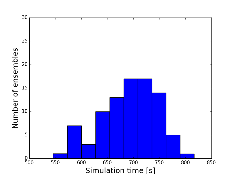
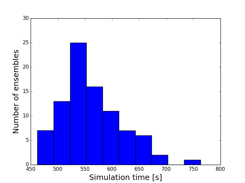
Figure 20: Histogram over simulation times for an ensemble of Norne realizations for OPM Flow (left) and ECLIPSE (right).

The individual simulations were run in serial mode on an Intel i7-6700 CPU @ 3.40 Ghz with 16 GiB memory. Figure 20 shows the resulting run time distributions. The mean run time for OPM Flow on the ensembles is 690 seconds, whereas for ECLIPSE it is 562 seconds, making OPM Flow approximately 25% slower than ECLIPSE on average. The ensemble is modified compared to the base case referred to in Section 3.7.1, so the results are not completely equivalent. We still expect that the difference can be reduced with aggressive compiler options and light tuning. Both simulators run through all ensemble members without having severe convergence issues. Tuning of numerical parameters such as tolerances can sometimes improve simulator performance. For this comparison, both simulators have been run with their respective default tuning parameters. Figure 21 report oil production results for a single well for the whole ensemble. Since unmatched realizations are used, there is a large spread in the results. This spread will typically be reduced if the models are constrained on the historical data using a history matching procedure.

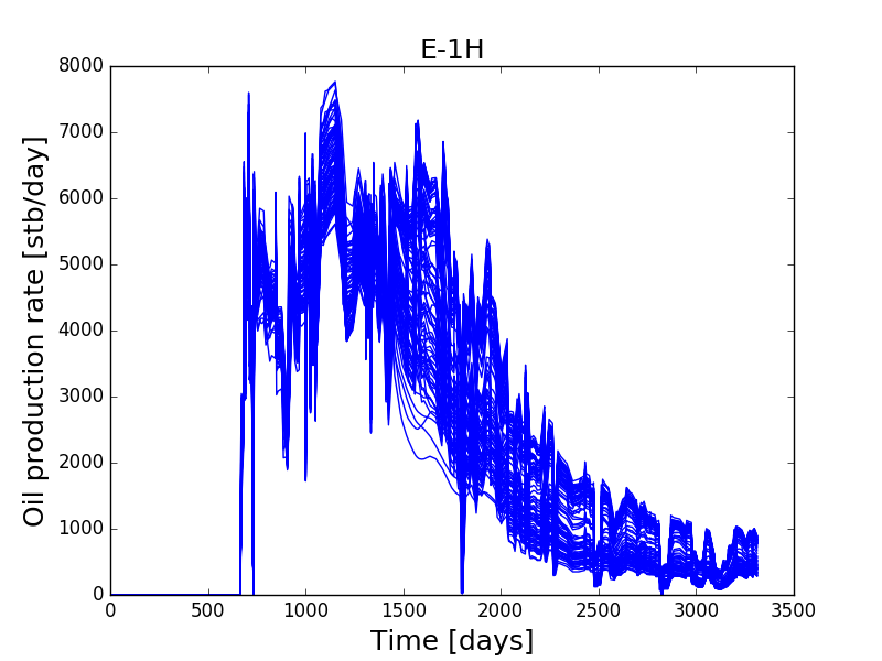
Figure 21: Oil production rates for 100 realizations of the Norne model.

4 Summary and Outlook

This paper has described OPM Flow at the time of writing. The software is under continuous development, so changes and additions should be expected. New features in development include adjoint calculations, higher-order discretizations in space and time [40], new fluid models for CO₂ behavior, and sequential implicit methods. We think that at this point OPM forms a robust base for both research and industrial applications, and that going forward this combination will help shorten the research cycle by giving researchers an industrial-strength platform on which to build and test their methods, as well as satisfying engineering requirements.

5 Acknowledgements

The authors thank Schlumberger for providing us with academic software licenses to ECLIPSE, used for comparing simulation results with OPM Flow. Work on OPM Flow and this article has been supported by Gassnova through the Climit Demo program and by Equinor.

Robert Klöfkorn, Tor Harald Sandve, and Ove Sævareid acknowledge the Research Council of Norway and the industry partners (ConocoPhillips Skandinavia AS, Aker BP ASA, Vår Energi AS, Equinor ASA, Neptune Energy Norge AS, Lundin Norway AS, Halliburton AS, Schlumberger Norge AS, and Wintershall DEA) of the National IOR Centre of Norway for support.

Appendix A Nomenclature

A.1 Symbol definitions for the continuous equations

$\phi$

porosity, can be a function of (oil) pressure: $\phi=m_{\phi}(p_{o})\phi_{\rm ref}$.

$m_{\phi}$

pore volume multiplier as function of pressure.

$\phi_{\rm ref}$

reference porosity, a constant in time but varying in space.

$p_{\alpha}$

phase pressure for phase $\alpha$.

$b_{\alpha}$

shrinkage/expansion factor for phase $\alpha$ defined as the ratio of surface volume at standard conditions to reservoir volume for a given amount of fluid: $b_{\alpha}=V_{\rm{surface},\alpha}/V_{\rm{reservoir},\alpha}$. For the oil phase, $b_{o}$ is called shrinkage factor, whereas $b_{g}$ is called expansion factor. The reciprocal quantity is called formation volume factor, and is usually denoted with a capital $B$: $B_{\alpha}=1/b_{\alpha}$. Usually a function of phase pressure and composition: $b_{\alpha}=b_{\alpha}(p_{\alpha},r_{go},r_{og})$. See Section 2.1.6.

$r_{go}$

ratio of dissolved gas to oil in the oleic phase. Often called $r_{S}$ in other literature.

$r_{og}$

ratio of vaporized oil to gas in the gaseous phase. Often called $r_{V}$ in other literature.

$s_{\alpha}$

saturation of phase $\alpha$, the pore volume fraction occupied by the phase. The saturations of all phases sum to 1.

$p_{c,\alpha\beta}$

capillary pressure between phases $\alpha$ and $\beta$. Typically a function of saturation: $p_{c,\alpha\beta}=p_{c,\alpha\beta}(s_{\alpha})$.

${\bf K}$

permeability of the porous medium.

$k_{r,\alpha}$

relative permeability for phase $\alpha$, modeling the reduction in effective permeability for a fluid phase in the presence of other phases. Typically a function of saturation, see Section 2.1.5.

$\mu_{\alpha}$

viscosity of phase $\alpha$, typically a function of phase pressure and composition.

$\lambda_{\alpha}$

mobility of phase $\alpha$, given by $\lambda_{\alpha}=k_{r,\alpha}/\mu_{\alpha}$.

${\bf v}_{\alpha}$

phase velocity of phase $\alpha$.

${\bf u}_{\alpha}$

component velocity of component $\alpha$.

$\rho_{S,\alpha}$

surface density of phase $\alpha$ at one atmosphere, a given constant.

$\rho_{\alpha}$

density of phase $\alpha$ in the reservoir. For water, $\rho_{w}=b_{w}\rho_{S,w}$. For the oleic phase the relationship is more complex since it must include dissolved gas: $\rho_{o}=b_{o}(\rho_{S,o}+r_{go}\rho_{S,g})$, similar for the gaseous phase: $\rho_{g}=b_{g}(\rho_{S,g}+r_{og}\rho_{S,o})$.

${\bf g}$

gravitational acceleration vector.

$q_{\alpha}$

well outflux density of pseudo component $\alpha$, (negative for well inflows). The form of this term depends on the well model used, see Section 2.2.

A.2 Symbol definitions for the discrete equations

$V$

cell volume.

$\Delta t$

time step length for the current Euler step.

$v_{\alpha}$

volume flux of phase $\alpha$ (oriented quantity).

$u_{\alpha}$

surface volume flux of pseudocomponent $\alpha$ (oriented quantity).

$T_{ij}$

transmissibility factor for a connection, derived from permeability, see B.

$m_{T}$

transmissibility multiplier as function of pressure.

$C(i)$

connections from cell $i$, i.e. the set of cells connected to it.

$U(\alpha,ij)$

upwind cell for phase $\alpha$ for the connection between cells $i$ and $j$.

$\Delta\Phi_{\alpha,ij}$

potential difference for phase $\alpha$ for the connection between cells $i$ and $j$ (oriented quantity).

$g$

gravitational acceleration in the $z$-direction.

$z_{i}$

depth of center of cell $i$.

A.3 Symbol definitions for the well models

$T_{w,j}$

connection transmissibility factor.

$M_{\alpha,j}$

the mobility for phase $\alpha$ at the connection $j$.

$p_{j}$

pressure of the grid block that contains the connection $j$.

$p_{bhp,w}$

the bottom-hole pressure of the well $w$.

$h_{w,j}$

pressure difference within the wellbore between connection $j$ and the well’s bottom-hole datum depth.

Appendix B Transmissibility

The transmissibility $T_{ij}$ of a connection between two cells is a discrete measure of the fluid flow capacity of that connection. We can define $T_{ij}$ by requiring that the discrete flow equations (9), (10), and (11) should be satisfied for a piecewise homogenous medium, by a velocity field satisfying Darcy’s law. For a single, incompressible fluid $b=1$ and the discrete equations reduce to

$$v_{ij}=\frac{1}{\mu}T_{ij}\big{(}p_{i}-p_{j}-g\rho_{ij}(z_{i}-z_{j})\big{)}.$$ (41)

We can ignore gravity since the formula must hold also normal to the gravity direction, and assume without loss of generality that the viscosity is 1, yielding the simplified discrete equation

$$v_{ij}=T_{ij}\big{(}p_{i}-p_{j}\big{)}$$ (42)

and the simplified Darcy law

$${\bf v}=-{\bf K}\nabla p.$$ (43)

Figure 22: Quantities used to compute the transmissibility between two cells.

Consider Figure 22, where ${\bf c}_{i}$ and ${\bf c}_{j}$ are the centroids of cells $i$ and $j$ and ${\bf c}_{ij}$ is the centroid of their common face $F_{ij}$. Then the flux $v_{ij}$ is given by

$$v_{ij}=\int_{F_{ij}}{\bf v}\cdot\hat{\bf n}_{ij}\,dA$$ (44)

where $\hat{\bf n}_{ij}$ is the unit normal of the face $F_{ij}$. This can be approximated by evaluating at the face centroid and using the Darcy formula (43) in each of the cells $i$ and $j$ by

$$v_{ij} =-|F_{ij}|(p_{ij}-p_{i})\frac{{\bf K}_{i}({\bf c}_{ij}-{\bf c}_{i})}{|{\bf c}_{ij}-{\bf c}_{i}|^{2}}\cdot\hat{\bf n}_{ij}, v_{ij} =-|F_{ij}|(p_{ji}-p_{j})\frac{{\bf K}_{j}({\bf c}_{ij}-{\bf c}_{j})}{|{\bf c}_{ij}-{\bf c}_{j}|^{2}}\cdot\hat{\bf n}_{ij},$$ (45)

where $|F_{ij}|$ is the area of the face $F_{ij}$ between cells $i$ and $j$, $p_{ij}$ is the pressure in cell $i$ at the point ${\bf c}_{ij}$, and $p_{ji}$ the pressure in cell $j$ at ${\bf c}_{ij}$. We then define the half-transmissibility $t_{ij}$ of cell $i$ with respect to $F_{ij}$ by

$$t_{ij} =|F_{ij}|\frac{{\bf K}_{i}({\bf c}_{ij}-{\bf c}_{i})}{|{\bf c}_{ij}-{\bf c}_{i}|^{2}}\cdot\hat{\bf n}_{ij}$$ (46)

with a similar definition for $t_{ji}$ notably using $\hat{\bf n}_{ji}=-\hat{\bf n}_{ij}$. Then

$$v_{ij}=-t_{ij}(p_{ij}-p_{i}),\qquad v_{ij}=t_{ji}(p_{ji}-p_{j}).$$ (47)

Requiring that the interface pressures $p_{ij}$ and $p_{ji}$ are equal, we get

$$v_{ij}=T_{ij}(p_{i}-p_{j})\qquad T_{ij}=\frac{t_{ij}t_{ji}}{t_{ij}+t_{ji}}$$ (48)

Finally, as a modeling tool one may multiply the transmissibilities by a pressure-dependent multiplier $m_{T}$. This can be used for example to model sub-scale features such as fractures opening and closing due to pressure changes, thereby changing overall permeability, without explicitly representing such fractures.

References

- [1] P. Bastian, M. Blatt, A. Dedner, C. Engwer, R. Klöfkorn, M. Ohlberger, O. Sander, A generic grid interface for parallel and adaptive scientific computing. Part I: Abstract framework, Computing 82 (2–3) (2008) 103–119. doi:10.1007/s00607-008-0003-x.
- [2] B. Flemisch, M. Darcis, K. Erbertseder, B. Faigle, A. Lauser, K. Mosthaf, S. Müthing, P. Nuske, A. Tatomir, M. Wolff, R. Helmig, DuMux: DUNE for multi-{phase,component,scale,physics,…} flow and transport in porous media, Advances in Water Resources 34 (9) (2011) 1102–1112. doi:10.1016/j.advwatres.2011.03.007.
- [3] E. G. Boman, U. V. Catalyurek, C. Chevalier, K. D. Devine, The Zoltan and Isorropia parallel toolkits for combinatorial scientific computing: Partitioning, ordering, and coloring, Scientific Programming 20 (2) (2012) 129–150. doi:10.3233/SPR-2012-0342.
- [4] K.-A. Lie, S. Krogstad, I. S. Ligaarden, J. R. Natvig, H. M. Nilsen, B. Skaflestad, Open-source matlab implementation of consistent discretisations on complex grids, Computational Geosciences 16 (2) (2011) 297–322. doi:10.1007/s10596-011-9244-4.
- [5] S. Krogstad, K.-A. Lie, O. Møyner, H. M. Nilsen, X. Raynaud, B. Skaflestad, MRST-AD - an open-source framework for rapid prototyping and evaluation of reservoir simulation problems, in: Reservoir simulation Symposium, Houston, Texas, USA, 23-25 February, 2015. doi:10.2118/173317-MS.
- [6] K.-A. Lie, An Introduction to Reservoir Simulation Using MATLAB/GNU Octave: User Guide for the MATLAB Reservoir Simulation Toolbox (MRST), Cambridge University Press, 2019. doi:10.1017/9781108591416.
- [7] O. Møyner, S. Krogstad, K.-A. Lie, The application of flow diagnostics for reservoir management, SPE J. 20 (2) (2014) 306–323. doi:10.2118/171557-PA.
- [8] R. D. Neidinger, Introduction to automatic differentiation and matlab object-oriented programming, SIAM Rev. 52 (3) (2010) 545–563. doi:10.1137/080743627.
- [9] J. Jansen, Adjoint-based optimization of multi-phase flow through porous media a review, Computers & Fluids 46 (1) (2011) 40–51, 10th ICFD Conference Series on Numerical Methods for Fluid Dynamics (ICFD 2010). doi:10.1016/j.compfluid.2010.09.039.
-
[10]
D. Baxendale, A. F. Rasmussen, A. B. Rustad, T. Skille, T. H. Sandve,
OPM Flow Documentation Manual, Open
Porous Media initiative, 2017.
URL opm-project.org/?page_id=955 - [11] J. E. Killough, Reservoir simulation with history-dependent saturation functions, SPE Journal 16 (1) (1976) 37–48. doi:10.2118/5106-PA.
- [12] F. M. Carlson, Simulation of relative permeability hysteresis to the non-wetting phase, in: SPE Annual Technical Conference & Exhibition, San Antonio, Texas, USA, Society of Petroleum Engineers, 1981. doi:10.2118/10157-MS.
- [13] J. Holmes, Enhancements to the strongly coupled, fully implicit well model: wellbore crossflow modeling and collective well control, in: SPE Reservoir Simulation Symposium, Society of Petroleum Engineers, 1983.
- [14] J. Holmes, T. Barkve, O. Lund, Application of a multisegment well model to simulate flow in advanced wells, in: European Petroleum Conference, Society of Petroleum Engineers, 1998.
- [15] R. M. Fonseca, E. Della Rossa, A. A. Emerick, R. G. Hanea, J. D. Jansen, Overview of the Olympus field development optimization challenge, in: ECMOR XVI-16th European Conference on the Mathematics of Oil Recovery, 2018. doi:10.3997/2214-4609.201802246.
- [16] J. Appleyard, I. M. Cheshire, Nested factorization, in: 7th SPE Symposium on Reservoir Simulation, San Francisco, USA, Society of Petroleum Engineers, 1983. doi:10.2118/12264-MS.
- [17] J. Wallis, Incomplete Gaussian Elimination as a Preconditioning for Generalized Conjugate Gradient Acceleration, in: 7th SPE Symposium on Reservoir Simulation, San Francisco, USA, Society of Petroleum Engineers, 1983. doi:10.2118/12265-MS.
- [18] R. Scheichl, M. Roland, J. Wendebourg, Decoupling and block preconditioning for sedimentary basin simulations, Computational Geosciences 7 (2003) 295–318.
- [19] M. Blatt, A parallel algebraic multigrid method for elliptic problems with highly discontinuous coefficients, Ph.D. thesis, Ruprecht–Karls–Universität Heidelberg (2010).
- [20] M. Blatt, P. Bastian, The Iterative Solver Template Library, in: B. Kågström, E. Elmroth, J. Dongarra, J. Waśniewski (Eds.), Applied Parallel Computing. State of the Art in Scientific Computing, Vol. 4699 of Lecture Notes in Computer Science, Springer, 2007, pp. 666–675.
- [21] M. Blatt, P. Bastian, On the generic parallelisation of iterative solvers for the finite element method, Int. J. Comput. Sci. Engrg. 4 (1) (2008) 56–69. doi:10.1504/IJCSE.2008.021112.
- [22] S. Balay, et al., PETSc users manual, Tech. Rep. ANL-95/11 - Revision 3.11, Argonne National Laboratory, www.mcs.anl.gov/petsc (2019).
- [23] A. Griewank, A. Walther, Evaluating Derivatives, Principles and Techniques of Algorithmic Differentiation, second edition, SIAM, Philadelphia, 2008.
- [24] A. Walther, A. Griewank, Getting started with ADOL-C, in: U. Naumann, O. Schenk (Eds.), Combinatorial Scientific Computing, Chapman-Hall CRC Computational Science, 2012, Ch. 7, pp. 181–202.
- [25] A. Lauser, A. F. Rasmussen, T. H. Sandve, H. M. Nilsen, Local forward-mode automatic differentiation for high performance parallel pilot-level reservoir simulation, in: ECMOR XVI-16th European Conference on the Mathematics of Oil Recovery, 2018. doi:10.3997/2214-4609.201802153.
- [26] P. Bastian, M. Blatt, A. Dedner, C. Engwer, R. Klöfkorn, R. Kornhuber, M. Ohlberger, O. Sander, A generic grid interface for parallel and adaptive scientific computing. Part II: Implementation and tests in DUNE, Computing 82 (2–3) (2008) 121–138. doi:10.1007/s00607-008-0004-9.
- [27] E. G. Boman, U. V. Catalyurek, C. Chevalier, K. D. Devine, The Zoltan and Isorropia parallel toolkits for combinatorial scientific computing: Partitioning, ordering, and coloring, Scientific Programming 20 (2).
- [28] K. D. Devine, E. G. Boman, R. T. Heaphy, R. H. Bisseling, U. V. Catalyurek, Parallel hypergraph partitioning for scientific computing, in: Proceedings 20th IEEE International Parallel & Distributed Processing Symposium, IEEE, 2006. doi:10.1109/IPDPS.2006.1639359.
- [29] U. Meier Yang, On the use of relaxation parameters in hybrid smoothers, Numer. Linear Algebra Appl. 11 (2–3) (2004) 155–172.
- [30] M. R. Todd, W. J. Longstaff, The development, testing, and application of a numerical simulator for predicting miscible flood performance, Journal of Petroleum Technology 24 (07) (1972) 874–882.
- [31] C. A. Chase Jr, M. R. Todd, Numerical simulation of CO2 flood performance (includes associated papers 13950 and 13964), SPE Journal 24 (06) (1984) 597–605.
- [32] S. Jakupsstovu, D. Zhou, J. Kamath, L. Durlofsky, E. H. Stenby, Upscaling of miscible displacement processes, in: Proceedings of the 6th Nordic Symposium on Petrophysics, 2001, pp. 15–16.
- [33] A. S. Odeh, Comparison of solutions to a three-dimensional black-oil reservoir simulation problem (includes associated paper 9741), Journal of Petroleum Technology 33 (01) (1981) 13–25.
- [34] D. Kenyon, Third SPE comparative solution project: gas cycling of retrograde condensate reservoirs, SPE Journal 39 (08) (1987) 981–997. doi:10.2118/12278-PA.
- [35] J. E. Killough, C. A. Kossack, Fifth comparison solution project: Evaluation of miscible flood simulators, in: SPE Symposium on Reservoir Simulation, 1987. doi:10.2118/16000-MS.
- [36] J. E. Killough, Ninth SPE comparative solution project: a reexamination of black-oil simulation, in: SPE Reservoir Simulation Symposium, Society of Petroleum Engineers, 1995. doi:10.2118/29110-MS.
- [37] K. Bao, K.-A. Lie, O. Møyner, M. Liu, Fully implicit simulation of polymer flooding with mrst, Computational Geosciences 21 (5) (2017) 1219–1244. doi:10.1007/s10596-017-9624-5.
- [38] T. H. Sandve, A. Rasmussen, A. B. Rustad, Open reservoir simulator for CO2 storage and CO2-EOR, in: 14th Greenhouse Gas Control Technologies Conference Melbourne, 2018, pp. 21–26.
- [39] R. Lorentzen, X. Luo, T. Bhakta, R. Valestrand, History matching Norne reservoir and petroelastic models using seismic impedance with correlated noise, SPE Journal 24 (4) (2019) 1452–1467. doi:10.2118/194205-PA.
- [40] A. Kvashchuk, R. Klöfkorn, T. H. Sandve, Comparison of higher order schemes on complicated meshes and reservoirs, in: SPE Reservoir Simulation Conference, Society of Petroleum Engineers, 2019. doi:10.2118/193839-MS.