Phase coexistence of active Brownian particles

Abstract

We investigate motility-induced phase separation of active Brownian particles, which are modeled as purely repulsive spheres that move due to a constant swim force with freely diffusing orientation. We develop on the basis of power functional concepts an analytical theory for nonequilibrium phase coexistence and interfacial structure. Theoretical predictions are validated against Brownian dynamics computer simulations. We show that the internal one-body force field has four nonequilibrium contributions: (i) isotropic drag and (ii) interfacial drag forces against the forward motion, (iii) a superadiabatic spherical pressure gradient and (iv) the quiet life gradient force. The intrinsic spherical pressure is balanced by the swim pressure, which arises from the polarization of the free interface. The quiet life force opposes the adiabatic force, which is due to the inhomogeneous density distribution. The balance of quiet life and adiabatic forces determines bulk coexistence via equality of two bulk state functions, which are independent of interfacial contributions. The internal force fields are kinematic functionals which depend on density and current, but are independent of external and swim forces, consistent with power functional theory. The phase transition originates from nonequilibrium repulsion, with the agile gas being more repulsive than the quiet liquid.

I Introduction

The spontaneous occurrence of gas-liquid phase separation into macroscopic bulk phases and the associated emergence of a stable interface between the two different fluids is one of the most striking phenomena in equilibrium statistical physics. It was Johannes van der Waals who first developed microscopic theories for both the bulk behaviour vanderWaals1873 and the interfacial structure vanderWaals1893 . Subsequently, Smoluchowski smoluchowski1908 and Mandelstam mandelstam1913 successfully described thermally excited capillary waves as collective fluctuations that generate interfacial roughness. The description of the free fluid interface constitutes one of the most challenging problems in statistical mechanics RowlinsonWidomBook ; Hansen06 ; evans1979 . It is relevant for the demixing of liquid mixtures zhang2018 ; ashton2011 , and it forms one of the most well-developed cornerstones of theoretical physics triezenberg72 ; weeks77 ; wertheim ; parry16 . Both advanced computer simulations chacon03prlIntrinsic and direct experimental observation, in e.g. colloid-polymer mixture aarts2004 , are means of investigation.

Given this situation in equilibrium, it seems natural to attempt to describe fluid interfaces in nonequilibrium on the basis of similar concepts. Examples of this strategy include the reduction of experimentally observed derks2008 interfacial roughness via shear flow as an effective confinement effect smith2008 . In the context of active fluids, which consist of self-driven particles, integrating out the swimming was shown to lead to an effective attraction between the particles farage2015effective , which then can be input into an equilibrium treatment of the interfacial structure, e.g. on the basis of classical density functional theory wittman2016interface .

Active Brownian particles have become a prototype for the study of nonequilibrium phenomena maggi2015 ; marconi2015towards . In particular their “motility-induced” phase separation into high- and low-density steady states continues to attract much current interest paliwal2018njp ; digregorio2018prl ; solon2018rapComm ; solon2018njp ; prymidis16activeLJ ; vanderMeer16activepassive . Very significant efforts have been devoted to understanding this phase transition, which occurs without any explicit interparticle attraction. This is a striking difference to the equilibrium gas-liquid case, where the balance of short-ranged repulsion and long-ranged intermolecular attraction drives a transition between the gas with high entropy and high energy and the liquid with low entropy and low energy. In contrast, for the motility-induced case, frequently a “feedback” mechanism is invoked in which particles in dense regions slow down feedback . The striking feature of the transition is the very strong inhomogeneity in density between the dense and the dilute phase. The challenge lies in understanding what physical mechanism would oppose the strong tendency of the liquid to expand and hence to homogenize the system. The homogenization does not occur, at strong enough driving conditions, such that nonequilibrium phase coexistence is stable.

That strong density inhomogeneities can spontaneously occur is well-known in equilibrium situations. Examples include adsorption of liquid or solid films on substrates and capillary condensation and freezing inside of narrow pores as well as nucleation phenomena lutsko . In these equilibrium cases balancing forces have been identified that act against the interparticle repulsion, be it intermolecular attraction, such as in the Lennard-Jones system, or via the influence of further species that generate effective attraction via the depletion mechanism. There are prominent cases, such as e.g. colloid-polymer mixtures, where fluid-fluid phase separation occurs in purely repulsive mixtures. In monocomponent system, the hard sphere fluid-solid (freezing) transition is a further prototype for coexistence of phases with differing spatial symmetries.

Often the interparticle repulsion is satisfactorily treated in a local way, assuming that high local density is associated with a free energy penalty that is taken to be a function of the local density. Nevertheless, much more sophisticated approximations exist within the framework of classical density functional theory, where a broad range of approximate functionals is available, ranging from square-gradient semi-local functionals to fully-nonlocal fundamental-measure Rosenfeld theories. When the system is driven out of equilibrium, then additional force contributions arise. In nonequilibrium, construction of the adiabatic state fortini14prl allows to systematically rationalize the force field that is solely due to the inhomogeneous density distribution, and subsequently analyse systematically the additional nonequilibrium (superadiabatic) forces.

Active phase separation is considered to be such a very striking phenomenon, as no apparent balancing mechanism, which would counteract the repulsion and keep the dense region compressed, has been identified. Nevertheless, a broad variety of different theoretical methods have been employed to study the phase separation phenomenon, which occurs very prominently and in a robust and reproducible way in Brownian dynamics (BD) computer simulations digregorio2018prl ; paliwal2018njp ; solon2018rapComm ; solon2018njp ; prymidis16activeLJ ; vanderMeer16activepassive . Among the different theoretical approaches are theories based on modified forms of the Cahn-Hilliard equation solon2018rapComm ; solon2018njp ; speck2014prl , hydrodynamic description stark2016sm , and more microscopic statistical mechanics treatments that start from the Smoluchowski equation of motion for the many-body probability distribution function paliwal2018njp . One closely related aim is to identify coexistence conditions and to construct a thermodynamic description of the system takatoriBrady2015thermodynamics . This is relevant as it allows to judge whether and if so which of the properties of equilibrium gas-liquid phase separation carry over to the nonequilibrium case. The most recent treatments conclude that interfacial effects affect the bulk coexistence paliwal2018njp ; solon2018rapComm ; solon2018njp , in striking contrast to the equilibrium case.

Here we study the bulk behaviour and interfacial structure of active Brownian particles in nonequilibrium steady states. We develop an analytical theory for the free interface between phase-separated bulk states of active Brownian particles. The theory is fully resolved in both position and orientation. The symmetry of the problem allows to reduce the dependence on one spatial coordinate ($x$) perpendicular to the interface and one angle ($\varphi$) of particle orientation against the $x$-axis. The theory describes correctly the orientational ordering at the interface, including dipolar and higher orientational moments. We validate the theoretical results for the force fields against (overdamped) BD simulation data of the phase separated system. Bulk phase coexistence occurs on the isotropic level of the correlation functions and the coexistence conditions are independent of interfacial effects. As an illustration, we show a BD simulation snapshot in Fig. 1(a), obtained for the frequently-used Weeks-Chandler-Anderson (WCA) repulsive pair potential $\phi(r)$ WCA1971 , as plotted in Fig. 1(b).

II Theory

II.1 Many-body dynamics

In the Langevin picture, the many-body dynamics of $N$ active Brownian particles are given by

$$\gamma\dot{\mathbf{r}}_{i} =-\nabla_{i}\sum_{j(\neq i)}\phi(|{\mathbf{r}}_{i}-{\mathbf{r}}_{j}|)+\gamma s{\boldsymbol{\omega}}_{i}+{\boldsymbol{\chi}}_{i},$$ (1)

where $\gamma$ is the friction constant against the static background, ${\mathbf{r}}_{i}(t)$ indicates the position of particle $i=1,\ldots,N$ at time $t$, the overdot indicates a time derivative, $\nabla_{i}$ indicates the derivative with respect to ${\mathbf{r}}_{i}$, $s=\rm const$ is the speed of free swimming (such that $\gamma s$ is the magnitude of the swim force), the unit vector ${\boldsymbol{\omega}}_{i}$ denotes the orientational degrees of freedom (along which the swim force acts) of particle $i$, and ${\boldsymbol{\chi}}_{i}(t)$ is a stochastic white noise force term, which is bias free, $\langle{\boldsymbol{\chi}}_{i}(t)\rangle=0$, and delta correlated with itself, $\langle{\boldsymbol{\chi}}_{i}(t){\boldsymbol{\chi}}_{j}(t^{\prime})\rangle=2k_{B}T\gamma\delta(t-t^{\prime}){\bf 1}\delta_{ij}$. Here the angles denote an average of the noise, $\bf 1$ denotes the $d\times d$ unit matrix, where $d$ is the space dimensionality, $k_{B}$ denotes the Boltzmann constant, and $T$ indicates absolute temperature; the translational diffusion constant is then given by $D=k_{B}T/\gamma$. In a system with $d=2$ space dimensions, as we consider below, the particle orientations can be parametrized by the angle $\varphi_{i}$ of particle orientation ${\boldsymbol{\omega}}_{i}$ against the $x$-axis, i.e. ${\boldsymbol{\omega}}_{i}=(\cos\varphi_{i},\sin\varphi_{i})$. The particle orientations diffuse freely, and hence

$$\gamma^{\omega}\dot{\varphi}_{i} =\chi_{i},$$ (2)

where $\chi_{i}(t)$ is an angular noise term with vanishing mean, $\langle\chi_{i}(t)\rangle=0$, and auto-correlation given by $\langle\chi_{i}(t)\chi_{j}(t^{\prime})\rangle=2k_{B}T\gamma^{\omega}\delta(t-t^{\prime})\delta_{ij}$. (For a description of rotational diffusion in $d=3$ see, e.g. farage2015effective .) For completeness, the rotational diffusion constant is then $D_{\rm rot}=k_{B}T/\gamma^{\omega}$. The BD simulations are based on the (standard) Euler algorithm for the system of equations (1) and (2) with time discretization step $\Delta t$.

II.2 Force density balance

We operate on the level of position- and orientation-resolved one-body fields: the one-body density $\rho({\mathbf{r}},{\boldsymbol{\omega}},t)$, the translational current ${\bf J}({\mathbf{r}},{\boldsymbol{\omega}},t)$, and the rotational current ${\bf J}^{\omega}({\mathbf{r}},{\boldsymbol{\omega}},t)$, where ${\mathbf{r}}$ denotes position, the unit vector ${\boldsymbol{\omega}}$ denotes the particle orientation along which the swimming force acts, and $t$ denotes time. The one-body fields are related by the exact (translational) force density balance,

$$\gamma{\bf J} =\gamma s{\boldsymbol{\omega}}\rho+{\bf F}_{\rm int}-k_{B}T\nabla\rho,$$ (3)

where the arguments ${\mathbf{r}},{\boldsymbol{\omega}},t$ of the three one-body fields ${\bf J},\rho$ and ${\bf F}_{\rm int}$ have been omitted for clarity. The force density balance (3) expresses the equality of the friction force density (left hand side) with the sum of the driving that generates the swimming (first term on the right hand side), the internal force density ${\bf F}_{\rm int}({\mathbf{r}},{\boldsymbol{\omega}},t)$ (second term), and the thermal diffusion (third term); see appendix A for a derivation from the many-body dynamics. The rotational motion alone is simple: Due to the free rotational diffusion (the particles are spherical), the rotational current is simply ${\bf J}^{\omega}({\mathbf{r}},{\boldsymbol{\omega}},t)=-D_{\rm rot}\nabla^{\omega}\rho({\mathbf{r}},{\boldsymbol{\omega}},t)$, where $D_{\rm rot}$ is the rotational diffusion constant, and $\nabla^{\omega}$ is the derivative in the space of orientations. The continuity equation is

$$\frac{\partial\rho}{\partial t}=-\nabla\cdot{\bf J}-\nabla^{\omega}\cdot{\bf J}^{\omega},$$ (4)

with $\partial\rho/\partial t=0$ in steady state.

The internal force density field, as occurring in (3), was proven to be a “kinematic” functional of the density and the current schmidt2013pft ; delasheras2018customFlow , i.e. ${\bf F}_{\rm int}({\mathbf{r}},{\boldsymbol{\omega}},t)={\bf F}_{\rm int}([\rho,{\bf J},{\bf J}^{\omega}],{\mathbf{r}},{\boldsymbol{\omega}},t)$. No further “hidden” dependence occurs; the internal force density field is in particular independent of external and swim forces. This theorem applies in general overdamped Brownian systems; see krinninger2016prl ; krinninger2019jcp for the generalization of power functional theory schmidt2013pft to rotator models, such as the current one.

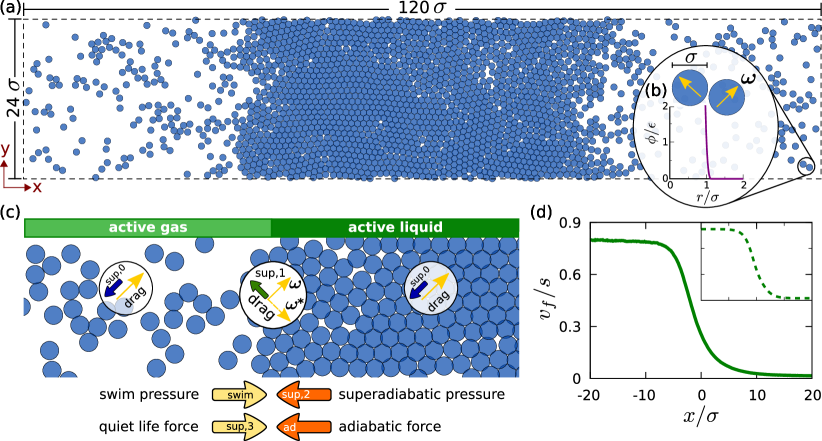
Figure 1: Overview of phase separated active Brownian particles. (a) Snapshot from BD simulations. The particles (blue) separate into regions with high and with low density. Due to periodic boundary conditions in $x$ and in $y$, two interfaces form along the short dimension of the simulation box with size $120\sigma$ in $x$ and $24\sigma$ in $y$. (b) Particles with size $\sigma$ at position ${\mathbf{r}}=(x,y)$ are driven in (unit vector) direction ${\boldsymbol{\omega}}$ by the swim force with strength $\gamma s$. The particles interact with the (WCA) repulsion $\phi(r)$ with energy scale $\epsilon$. (c) Illustration of the different one-body force density contributions that add up to the total internal force density field ${\bf F}_{\rm int}$: the drag force density ${\bf F}_{\rm sup,0}$ acts against the local current direction ${\bf J}$ and its magnitude is small (large) in the dilute (dense) phase. The non-spherical drag correction ${\bf F}_{\rm sup,1}$ occurs at the interface and it acts in direction ${\boldsymbol{\omega}}^{*}$ (${\boldsymbol{\omega}}$ mirrored at the $x$-axis). The swim pressure (orange arrow) is due to the polarization of the interface and it is balanced by the superadiabatic pressure (red arrow), which is low (high) in the dilute (dense) phase. The arrows indicate the direction of the respective negative pressure gradient. The quiet life force field ${\bf F}_{\rm sup,3}/\rho$ compresses the liquid and acts against the adiabatic force field ${\bf F}_{\rm ad}/\rho$, which is (solely) due to the density gradient and tends to expand the liquid. (d) Mean scaled forward swimming speed $v_{\rm f}/s$ as a function of the scaled position $x/\sigma$ across the interface in a phase-separated system of active Brownian particles interacting with the WCA pair potential, with particle size $\sigma$ and energy scale $\epsilon$. Simulation data are shown for $k_{B}T/\epsilon=0.5$ and $s{\color[rgb]{0,0,0}\tau}/\sigma=60$, where the timescale is $\tau=\sigma^{2}\gamma/\epsilon$, which corresponds to ${\rm Pe}=120$. The aspect ratio of the simulation box is 5 and the number $N$ of particles per system volume $V$ is $N/V=0.7\sigma^{-2}$ with $N=2000$; the time step is $\Delta t/\tau=10^{-5}$. Sampling was performed over $10^{8}$ time steps; see krinninger2019jcp for further simulation details that also apply to the present study. The inset shows the theoretical result (38). The inset axis labels have been omitted for clarity; the scale is identical to that of the main plot.

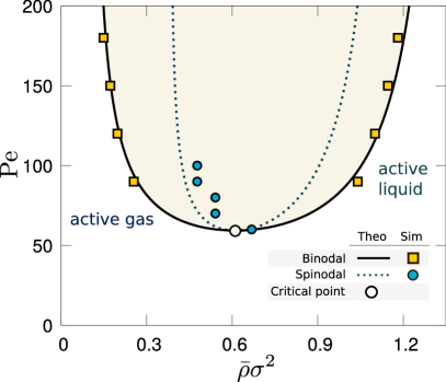
Figure 2: Nonequilibrium phase diagram as a function of scaled density $\rho_{\rm b}\sigma^{2}$ and Peclet number $\rm Pe$. Shown are the nonequilibrium binodal (solid line) and spinodal (dashed line) obtained from the present theory, compared to results for the binodal (orange squares) taken from Ref. paliwal2018njp , and for the gas side of the spinodal (blue circles) taken from Ref. stenhammar2013 . Also shown is the theoretical result for the critical point (open circle).

The internal force density field splits into a sum of adiabatic and superadiabatic contributions,

$${\bf F}_{\rm int} ={\bf F}_{\rm ad}+{\bf F}_{\rm sup},$$ (5)

where ${\bf F}_{\rm ad}$ is the force density in a corresponding “adiabatic” system. The adiabatic system is in equilibrium and constructed in such a way that its one-body density profile is identical to that of the true nonequilibrium system. The Mermin-Evans theorem of classical density functional theory evans1979 ensures that an external potential exists in the adiabatic system that accomplishes this task. We give a brief summary of classical density functional theory in appendix B. Crucially ${\bf F}_{\rm ad}$ depends (functionally) only on the density profile and not on the external force field. Furthermore ${\bf F}_{\rm ad}$ is independent of the (translational and rotational) current. The splitting (5) is exact; it is a consequence of the power functional variational framework schmidt2013pft ; krinninger2019jcp , and it was explicitly demonstrated in computer simulation work fortini14prl . In contrast to the adiabatic contribution, the superadiabatic force density profile ${\bf F}_{\rm sup}$ is a functional of the current (in the present case translational current and rotational current) as well as of the density profile.

The excess adiabatic force density field can be expressed as ${\bf F}_{\rm ad}=-\rho\nabla\delta F_{\rm exc}[\rho]/\delta\rho$, with the excess (over ideal gas) Helmholtz free energy density functional $F_{\rm exc}[\rho]$ evans1979 , see appendix B. For the present spherically repulsive interparticle interaction potential, ${\bf F}_{\rm ad}$ describes the repulsion that is solely due to the inhomogeneous density distribution. The genuine nonequilibrium contribution in (5) is the superadiabatic force density profile ${\bf F}_{\rm sup}$. Power functional theory schmidt2013pft ; krinninger2019jcp ensures that ${\bf F}_{\rm sup}$ depends both on the density profile and on the current distribution, but not explicitly on the external force field.

We proceed by splitting the total superadiabatic force density distribution into four different parts

$${\bf F}_{\rm sup} ={\bf F}_{\rm sup,0}+{\bf F}_{\rm sup,1}+{\bf F}_{\rm sup,2}+{\bf F}_{\rm sup,3},$$ (6)

where the contributions ${\bf F}_{\rm sup,0},{\bf F}_{\rm sup,1}$ and ${\bf F}_{\rm sup,2}$ are obtained via projection of ${\bf F}_{\rm int}$ onto a corresponding relevant orientation in the system and suitable averaging. The remainder is then contained in ${\bf F}_{\rm sup,3}$, and hence (6) does not constitute an approximation. The mathematical structure of each superadiabatic term in (6) is unique and characterizes a specific physical effect. The projections are performed by the correlator expressions for ${\bf F}_{\rm sup,0}$, ${\bf F}_{\rm sup,1}$, and ${\bf F}_{\rm sup,2}$, which are given and discussed below in (31), (34) and (41), respectively. Here we first briefly discuss these individual terms before going into more detail.

The drag force density ${\bf F}_{\rm sup,0}$ acts against the local flow direction. It leads to slowing of the forward swimming due to collisions of the particle at position ${\mathbf{r}}$ with surrounding particles. The strength of this effect increases the more crowded the environment is. The interfacial drag force density ${\bf F}_{\rm sup,1}$ is an orientation-dependent interfacial contribution with “tensorial” character, i.e. this drag force is not directed strictly against the forward motion, but takes account of the gradient direction in the system. This effect is induced by the inhomogeneous environment at the interface.

The force density field ${\bf F}_{\rm sup,2}$ is the negative gradient of an intrinsic spherical pressure $\Pi_{2}$. Characteristically $\Pi_{2}$ is independent of orientation ${\boldsymbol{\omega}}$. As a result the corresponding force density ${\bf F}_{\rm sup,2}=-\nabla\Pi_{2}$ is also independent of ${\boldsymbol{\omega}}$. Similarly, the quiet life force field ${\bf F}_{\rm sup,3}/\rho$ is the (negative) gradient of a spherical (nonequilibrium) chemical potential $\nu_{3}$, i.e. ${\bf F}_{\rm sup,3}/\rho=-\nabla\nu_{3}$. All superadiabatic contributions describe repulsion and occur due to the nonequilibrium driving in the system. We show below how these repulsive forces generate stable phase coexistence. As we demonstrate, in particular the quiet life force stabilizes the nonequilibrium bulk phase coexistence. It tends to push particles into the liquid where the mean velocity is low (towards the “quiet life”). Except for the bulk contribution to ${\bf F}_{\rm sup,0}$, neither of the internal force density contributions has been identified before. Figure 1(c) displays a schematic overview of all forces that act in the system.

The motion in the system is characterized by the forward current profile $J_{\rm f}(x)$, defined as an angular average of the projection of the current ${\bf J}$ onto the particle orientation ${\boldsymbol{\omega}}$,

$$J_{\rm f} =\frac{1}{2\pi}\int d{\boldsymbol{\omega}}{\bf J}\cdot{\boldsymbol{\omega}}.$$ (7)

The corresponding forward swimming speed profile $v_{\rm f}(x)$ is then obtained simply via

$$v_{\rm f} =J_{\rm f}/\rho_{0},$$ (8)

where the angular average of the density profile is defined as $\rho_{0}=\int d{\boldsymbol{\omega}}\rho/(2\pi)$. As an illustration, we show in Fig. 1(d) BD results for $v_{\rm f}$ as a function of $x$ across the interface in the phase separated system. The forward speed is high in the gas and low in the liquid fily2012prl ; stenhammar2013 and it crosses over smoothly between these plateau values as $x$ is varied from one phase to the other.

The plateau values of the forward speed $v_{\rm f}$ are described with good accuracy by the well-known simple linear decrease of the mean speed $v_{\rm b}$ with mean density $\rho_{\rm b}$ fily2012prl ; stenhammar2013 ; solon2015prl , given by

$$\frac{v_{\rm b}}{s}=1-\frac{\rho_{\rm b}}{\rho_{\rm jam}},$$ (9)

where $\rho_{\rm jam}$ is a constant that controls the slope of the decrease of the mean swim speed in bulk, as well as the upper limit of density (“jamming”). Here we take the convention that $\rho_{\rm b}$ indicates the number of particles per volume and per radians, hence $2\pi\rho_{\rm b}$ is the number of particles per two-dimensional volume.

In order to address the total force density balance (3), we specify the internal force splitting (5) and (6) further by requiring that

$$-k_{B}T\nabla\rho+{\bf F}_{\rm ad}+{\bf F}_{\rm sup,3} =0,$$ (10)

which yields upon inserting into (3) the relationship

$$\gamma{\bf J} =\gamma s{\boldsymbol{\omega}}\rho+{\bf F}_{\rm sup,0}+{\bf F}_{\rm sup,1}+{\bf F}_{\rm sup,2},$$ (11)

containing the motion (left hand side) and the contribution due to the swimming (first term on the right hand side). We will below identify the superadiabatic force fields that determine via (11) the flow that occurs in the system. Before doing so, in the following we first address the structural force density balance (10), which we will demonstrate to be a gradient relation when written in force field form.

II.3 Phase behaviour

In order to address nonequilibrium phase coexistence, we turn our description from force densities to force fields. We hence divide (10) by the orientation- and position-resolved density distribution $\rho$, which yields

$$-k_{B}T\nabla\ln\rho_{0}+{\bf f}_{\rm ad}({\mathbf{r}})+{\bf f}_{\rm sup,3}({\mathbf{r}}) =0,$$ (12)

where the adiabatic and superadiabatic force fields are defined by ${\bf f}_{\rm ad}={\bf F}_{\rm ad}/\rho$ and ${\bf f}_{\rm sup,3}={\bf F}_{\rm sup,3}/\rho$, respectively. For simplicity, we have replaced in (12) the ideal diffusion term $-k_{B}T\nabla\ln\rho$ by the corresponding isotropic component $-k_{B}T\nabla\ln\rho_{0}$. This is a good approximation, as we find that the difference between isotropic and anisotropic gradients is a small correction for relevant conditions, typically one or two orders smaller in magnitude compared to all other contributions footnote2 .

The adiabatic force field can be expressed as the negative gradient of the local excess (over ideal gas) chemical potential, which within classical density functional theory evans1979 ; evans2016 (see appendix B for a brief overview) is given via functional differentiation of the excess Helmholtz free energy functional $F_{\rm exc}[\rho_{0}]$,

$${\bf f}_{\rm ad}({\mathbf{r}}) =-\nabla\frac{\delta F_{\rm exc}[\rho_{0}]}{\delta\rho_{0}}.$$ (13)

Here the adiabatic state is an equilibrium system that possesses the same density distribution as the real system. The real and the adiabatic system share the same interparticle interaction potential. The orientational degrees of freedom do not affect the internal forces in equilibrium, as the particles are simple repulsive disks. Hence, the free energy functional requires only the average density profile $\rho_{0}$ as an input footnote4 , and ${\bf f}_{\rm ad}$ is independent of orientations. (This situation is different in a system of e.g. swimming rods or general anisotropic interparticle interactions.) An equivalent alternative to the density functional theory expression (13) is ${\bf f}_{\rm ad}=-\langle\nabla_{i}u({\mathbf{r}}^{N})\rangle_{\rm eq}$, where $u({\mathbf{r}}^{N})$ is the interparticle interaction potential. Here the equilibrium average is performed under the influence of a (hypothetical) “adiabatic” external potential $V_{\rm ad}({\mathbf{r}})$, chosen such that the resulting one-body density distribution $\rho$ is the correct one. In practice, this method requires to perform the average in e.g. Monte Carlo simulations fortini14prl ; delasheras2018customFlow .

In order to describe the adiabatic force field, we use a simple local density approximation, based on scaled-particle theory for two-dimensional hard disks (although more accurate approximations exist santos1995 ),

$${\bf f}_{\rm ad} =-\nabla\mu_{\rm ad},$$ (14)

where the chemical potential $\mu_{\rm ad}$ for a bulk fluid of density $\rho_{\rm b}$ is given by

$$\mu_{\rm ad}(\rho_{\rm b}) =k_{B}T\left[-\ln(1-\eta^{\prime})+\eta^{\prime}\frac{3-2\eta^{\prime}}{(1-\eta^{\prime})^{2}}\right].$$ (15)

Here we have introduced a rescaled packing fraction $\eta^{\prime}=0.8\eta$ in order to approximately take account of the repulsive sphere character of the system; in our units $\eta=\rho_{\rm b}/\rho_{\rm jam}$. Furthermore the bulk density $\bar{\rho}=N/V=2\pi\rho_{\rm b}$ indicates the number of particles per unit volume. The corresponding expression for the pressure can be obtained by integrating the thermodynamical relation $\partial P_{\rm ad}/\partial\rho_{\rm b}=\rho_{\rm b}\partial\mu_{\rm ad}/\partial\rho_{\rm b}$ in $\rho_{\rm b}$. This yields

$$P_{\rm ad}(\rho_{\rm b}) =k_{B}T\rho_{\rm b}\Big{[}\frac{1}{(1-\eta^{\prime})^{2}}-1\Big{]}.$$ (16)

The pressure generates the adiabatic force density, via a gradient operation, $\rho_{\rm b}{\bf f}_{\rm ad}=-\nabla P_{\rm ad}.$ The existence of the adiabatic force field and its corresponding integrals $\mu_{\rm ad}$ and $P_{\rm ad}$ is not that of an approximation. Rather this constitutes the part of the total nonequilibrium internal force density (and its corresponding position integrals) that is independent of velocity and hence dependent only on the density distribution (i.e. is a density functional). The “genuine” nonequilibrium contributions do also depend on the velocity field and are referred to as superadiabatic. We address the superadiabatic force fields in the following.

As ${\bf f}_{\rm ad}$ is independent of orientation, ${\bf f}_{\rm sup,3}$ also necessarily needs to be independent of ${\boldsymbol{\omega}}$, in order to satisfy (12). Furthermore, the adiabatic force field is a gradient field, due to (13). Hence in order for the force balance (12) to hold, the superadiabatic force field ${\bf f}_{\rm sup,3}$ necessarily also needs to be of gradient form,

$${\bf f}_{\rm sup,3} =-\nabla\nu_{3},$$ (17)

where $\nu_{3}(x)$ is the negative spatial integral of the force field.

We first address the value of $\nu_{3}$ for constant density $\rho_{\rm b}$, i.e. far from the interface, where all gradients vanish. Here we postulate an explicit form, which is quadratic in velocity, given by

$$\nu_{3}(\rho_{\rm b}) =e_{1}\frac{\gamma}{2D_{\rm rot}}v_{\rm b}^{2}\frac{\rho_{\rm b}}{\rho_{\rm jam}},$$ (18)

where $e_{1}$ is a (dimensionless) constant that controls the strength of the effect. Here our approximation (18) for $\nu_{3}$ depends on density and velocity, but not directly on $s$, as is consistent with the power functional framework schmidt2013pft . We find that using the form (18) we are able to satisfy the requirement that ${\bf F}_{\rm sup,3}$ is the remainder in the superadiabatic force splitting (6) in that no significant unexplained force contributions remain as compared to the simulation data. The magnitude of the observed numerical deviations is entirely consistent with the approximate nature of the expressions in our standalone theory.

Using the explicit expression (9) for $v_{\rm b}(\rho_{\rm b})$ allows to obtain a corresponding pressure contribution $\Pi_{3}$ via integration of $\partial\Pi_{3}/\partial\rho_{\rm b}=\rho_{\rm b}\partial\nu_{3}/\partial\rho_{\rm b}$. The result is

$$\Pi_{3}(\rho_{\rm b}) =\frac{\gamma e_{1}}{4D_{\rm rot}\rho_{\rm jam}}v_{\rm b}^{2}\rho_{\rm b}^{2}\left[1+\frac{\rho_{\rm b}(3\rho_{\rm b}-4\rho_{\rm jam})}{6(\rho_{\rm jam}-\rho_{\rm b})^{2}}\right].$$ (19)

In order to obtain the quantities that determine nonequilibrium phase coexistence, we return to the force balance relation (12), which we rewrite using the gradient expressions (14) and (17) as

$$-\nabla(k_{B}T\ln\rho_{0}+\mu_{\rm ad}+\nu_{3}) =0.$$ (20)

As the total gradient vanishes, the expression in brackets needs to be equal to a constant, $\mu=\rm const$, which plays the role of the total chemical potential. Similarly, the force density balance relation (10) can be rewritten as

$$-\nabla(k_{B}T\rho_{0}+P_{\rm ad}+\Pi_{3}) =0,$$ (21)

which again implies that the expression in brackets is constant, where the constant, $P=\rm const$, plays the role of the total pressure. The three individual terms inside of the gradient on the left hand side of (21) depend in general on position $x$. As before, $\rho_{0}(x)$ is the isotropic Fourier component of the density profile.

We can now define bulk values of the total chemical potential $\mu$ and the total pressure $P$ by summing up the individual contributions,

$$\mu(\rho_{\rm b}) =k_{B}T\ln\rho_{\rm b}+\mu_{\rm ad}+\nu_{3},$$ (22)

$$P(\rho_{\rm b}) =k_{B}T\rho_{\rm b}+P_{\rm ad}+\Pi_{3}.$$ (23)

We show below that although further contributions to the chemical potential exist, the sum of these additional contributions vanishes. Hence (22) indeed defines the total chemical potential. The same holds true for the total pressure, where we demonstrate below that although there is a swim pressure contribution, this is identically cancelled by a corresponding superadiabatic (i.e. intrinsic nonequilibrium) pressure that the system develops. Hence (23) represents the total pressure in nonequilibrium bulk steady states.

Phase coexistence implies that the densities in the coexisting gas and liquid phases, $\rho_{\rm g}$ and $\rho_{\rm l}$, respectively, satisfy

$$\mu(\rho_{\rm g}) =\mu(\rho_{\rm l}),$$ (24)

$$P(\rho_{\rm g}) =P(\rho_{\rm l}).$$ (25)

Equations (24) and (25), together with (22) and (23), (15) and (16), and (18) and (19), form a closed set of equations for the determination of the binodal densities $\rho_{\rm g}$ and $\rho_{\rm l}$, which we solve numerically. Figure 2 presents the theoretical results for the phase diagram, and comparison to simulation data from the literature. Here we have chosen $e_{1}=0.0865$ and $\rho_{\rm jam}2\pi\sigma^{2}=1.146$. The phase diagram possesses a lower, in Peclet number ${\rm Pe}\equiv 3s/(\sigma D_{\rm rot})=\gamma s\sigma/(k_{B}T)$, critical point (which is characterized by mean-field exponents within the present approach; see Ref. binder2018 for a simulation study of the critical scaling.) The binodal agrees very well with the simulation data of Ref. paliwal2018njp . We obtain the spinodal via the condition $\partial\mu(\rho_{\rm b})/\partial\rho_{\rm b}=0.$ The critical point is then obtained by the additional condition $\partial^{2}\mu/\partial\rho_{\rm b}^{2}=0$. This necessitates finding the appropriate root of a fourth-order polynomial in the value of the critical density footnote3 . We perform this task numerically.

We show in Fig. 2 the theoretical result for the spinodal density, together with the simulation data for the gas side of the spinodal by Stenhammar et al. stenhammar2013 . Clearly, the agreement between the theoretical results and the simulation data is very satisfactory. The theory in particular captures correctly the fact that the gas side of both the spinodal and the binodal remain at relatively large density upon increasing $\rm Pe$. This is in striking contrast to typical equilibrium gas-liquid coexistence, where the gas becomes rapidly very dilute upon increasing distance (in temperature) from the critical point.

Having established the bulk phase diagram, in the following we develop a microscopic theory for the interfacial structure between coexisting active gas and active liquid states. This allows us to demonstrate (i) that the sum of all further contributions to the state functions $\mu(\rho_{\rm b})$ and $P(\rho_{\rm b})$ indeed vanishes, and hence that (22) and (23) are complete, and (ii) that bulk coexistence is unaffected by interfacial contributions.

II.4 Fourier decomposition

We restrict ourselves to steady states of two-dimensional systems, which are spatially inhomogeneous only in the $x$-direction; orientation is measured by the angle $\varphi$ against the $x$-axis, i.e. ${\boldsymbol{\omega}}=(\cos\varphi,\sin\varphi)$. We Fourier decompose the kinematic fields $\rho$ and ${\bf J}$ according to

$$\rho(x,\varphi) =\sum_{n=0}^{\infty}\rho_{n}(x)\cos(n\varphi),$$ (26)

$$J_{x}(x,\varphi) =\sum_{n=1}^{\infty}J_{n}^{x}(x)\cos(n\varphi),$$ (27)

$$J_{y}(x,\varphi) =\sum_{n=1}^{\infty}J_{n}^{y}(x)\sin(n\varphi),$$ (28)

where the Cartesian components of the one-body current are $(J_{x},J_{y})\equiv{\bf J}$ and $\rho_{n}$, $J_{n}^{x}$, $J_{n}^{y}$ are Fourier coefficients which depend on position $x$. Terms that vanish due to symmetry in $\varphi$ have been omitted: the system is invariant under reflection with respect to the $x$-axis, i.e. under the joint coordinate transformation $y\to-y$ and $\varphi\to-\varphi$. Hence the density (26) and the $x$-component of the current (27) need to be even in $\varphi$; the $y$-component of the current (28) flips its direction under the reflection, and hence it is odd in $\varphi$. Furthermore, as is common, we restrict ourselves to cases where the isotropic current component vanishes, $J_{0}^{x}=J_{0}^{y}=0$. Using the low-order Fourier coefficients $n=0,1$, we can express frequently used standard observables: the orientation-integrated density distribution is simply $2\pi\rho_{0}$ and the polarization profile with respect to the $x$-axis is $\pi\rho_{1}$. Finally, we use the convention that $x=0$ indicates the position of the Gibbs dividing surface Hansen06 .

In the present case the rotational derivative $\nabla^{\omega}$ is simply $\partial/\partial\varphi$ and the general continuity equation (4) reduces to

$$\frac{\partial J_{x}}{\partial x} =D_{\rm rot}\frac{\partial^{2}\rho}{\partial\varphi^{2}}.$$ (29)

Upon inserting the Fourier ansatz (26) and (27), this can be cast into a relationship for the Fourier coefficients of the density of order $n\geq 1$,

$$\rho_{n} =-\frac{1}{n^{2}D_{\rm rot}}\frac{dJ_{n}^{x}}{dx},$$ (30)

which we will use below in order to derive a set of (coupled) differential equations for the Fourier coefficients.

II.5 Drag forces

In order to address the dynamical force balance (11), we specify the superadiabatic contributions in (6) further, by requiring that the drag force density ${\bf F}_{\rm sup,0}$ acts against the flow direction, and is given by an orientational average, defined by the correlator

$${\bf F}_{\rm sup,0} =\frac{{\bf J}}{2\pi J_{\rm f}}\int d{\boldsymbol{\omega}}^{\prime}{\boldsymbol{\omega}}^{\prime}\cdot{\bf F}_{\rm int}({\mathbf{r}},{\boldsymbol{\omega}}^{\prime}).$$ (31)

where the local orientation-averaged forward current profile $J_{\rm f}(x)$ is defined via (7) and ${\boldsymbol{\omega}}^{\prime}$ is a new angular integration variable. In the present two-dimensional system the integration over orientation space is simply $\int d{\boldsymbol{\omega}}\equiv\int_{-\pi}^{\pi}d\varphi$. The force density field ${\bf F}_{\rm sup,0}({\mathbf{r}},{\boldsymbol{\omega}})$ depends on orientation ${\boldsymbol{\omega}}$ via the dependence of ${\bf J}$ on ${\boldsymbol{\omega}}$ on the right hand side.

In order to develop the theory, we assume the drag force density (31) to have the form

$${\bf F}_{\rm sup,0} =-\frac{\gamma\rho_{0}}{\rho_{\rm jam}-\rho_{0}}[1+\xi(\nabla\rho_{0})^{2}]{\bf J},$$ (32)

where $\xi>0$ is a constant (with units of ${\rm length}^{2}/{\rm density}^{2}$) that determines the strength of the square gradient correction. For the case of constant density, $\nabla\rho_{0}=0$, the expression (32) reduces to the previously formulated bulk fluid drag force krinninger2016prl , which reproduces the well-known fily2012prl ; stenhammar2013 ; solon2015prl linear decrease (9) of the mean speed with increasing average density in bulk. Equation (32) constitutes a kinematic functional (i.e. the dependence is on $\rho$ and ${\bf J})$, as required schmidt2013pft ; krinninger2016prl .

In order to describe the orientation-averaged density profile across the interface, we use the classic form

$$\rho_{0}(x) =\frac{\rho_{\rm l}+\rho_{\rm g}}{2}+\frac{\rho_{\rm l}-\rho_{\rm g}}{2}\tanh(x/\lambda),$$ (33)

where the lengthscale $\lambda$ determines the width of the interface. The corresponding mean densities, with units of particle number per system volume, are $2\pi\rho_{\rm g}$ and $2\pi\rho_{\rm l}$. Equation (33) is widely used in the description of the present problem paliwal2018njp ; paliwal2017jcp and it is considered to be an excellent approximation to simulation results.

We next identify the non-spherical drag correction, defined by

$${\bf F}_{\rm sup,1} =\frac{{\boldsymbol{\omega}}^{*}}{2\pi}\int d{\boldsymbol{\omega}}^{\prime}({\bf F}_{\rm int}^{\prime}-{\bf F}_{\rm sup,0}^{\prime})\cdot{\boldsymbol{\omega}}^{\prime*},$$ (34)

where ${\boldsymbol{\omega}}^{*}=(\cos\varphi,-\sin\varphi)$ is the orientation ${\boldsymbol{\omega}}$ reflected at the $x$-axis. (Note that when viewing the set of $xy$-coordinates as the complex plane, then ${\boldsymbol{\omega}}^{\ast}$ is the complex conjugate to ${\boldsymbol{\omega}}$.) Furthermore, the primed force density fields inside of the orientation integral are evaluated at direction ${\boldsymbol{\omega}}^{\prime}$. In the theory, we postulate the nonspherical drag to have the form footnote5 :

$${\bf F}_{\rm sup,1} =-\frac{\gamma}{4}\rho_{1}v_{\rm f}\frac{1+\xi(\nabla\rho_{0})^{2}\rho_{0}/\rho_{\rm jam}}{1-\rho_{0}/\rho_{\rm jam}}{\boldsymbol{\omega}}^{*},$$ (35)

which is linear in the forward speed $v_{\rm f}$, as is appropriate for a drag term, and contains a square density gradient contribution to its amplitude. The direction of the nonspherical drag is against the ${\boldsymbol{\omega}}^{\ast}$ direction.

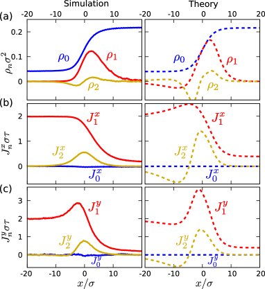
Figure 3: Representative Fourier coefficients obtained from BD simulation (left panels) and theory (right panels). Shown are Fourier components of order $n=0,1,2$ (as indicated) as a function of $x/\sigma$ for (a) the density $\rho_{n}\sigma^{2}$, (b) the $x$-component of the current, $J_{n}^{x}\sigma\tau$, and (c) the $y$-component of the current, $J_{n}^{y}\sigma\tau$, where the “molecular” timescale is $\tau=\gamma\sigma^{2}/\epsilon$. The simulation parameters are identical to those of Fig. 1.

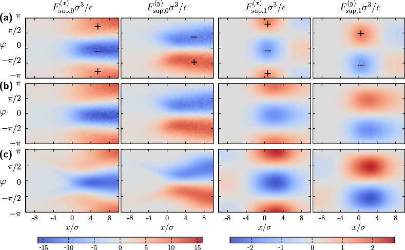
Figure 4: Spherical drag force density ${\bf F}_{\rm sup,0}$ and nonspherical drag force density ${\bf F}_{\rm sup,1}$, obtained from (a) simulations via correlators, (b) via kinematic functionals using simulation data as input, and (c) stand-alone theory. Shown are the $x-$ and $y-$components of the respective force density field: $F_{\rm sup,0}^{(x)}$ (first column) $F_{\rm sup,0}^{(y)}$ (second column), $F_{\rm sup,1}^{(x)}$ (third column), and $F_{\rm sup,1}^{(y)}$ (fourth column) in units of $\epsilon/\sigma^{3}$ and as a function of distance $x/\sigma$ across the interface and angle $\varphi$ with respect to the interface normal (pointing towards the liquid). The plus and minus signs indicate the sign of the force density fields.

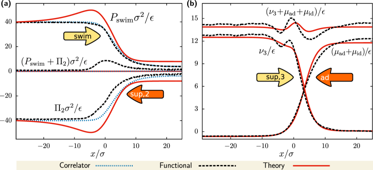
Figure 5: (a) Superadiabatic spherical pressure profile $\Pi_{2}(x)$, swim pressure profile $P_{\rm swim}(x)$, and the sum $\Pi_{2}(x)+P_{\rm swim}$, in units of $\epsilon/\sigma^{2}$ as a function of distance $x/\sigma$ across the interface. Results are obained from the correlator expressions using simulation data as input (blue dotted lines), from the kinematic functionals with simulation data input (black dashed lines) and from the stand alone theory (red solid lines). (b) Superadiabatic spherical chemical potential profile $\nu_{3}(x)$, the sum of adiabatic excess and ideal chemical potential profile $\mu_{\rm id}(x)+\mu_{\rm ad}(x)$, and the total chemical potential, i.e. the sum $\nu_{3}+\mu_{\rm ad}+\mu_{\rm id}$ in units of $\epsilon$ and as a function of $x/\sigma$. Here the ideal chemical potential is $\mu_{\rm id}=k_{B}T\ln(\eta^{\prime})$ with the local rescaled packing fraction $\eta^{\prime}=0.8\rho_{\rm b}/\rho_{\rm jam}$. For clarity the results for the sum have been shifted upwards by two units. The superadiabatic results are obtained using the kinematic functional with either the simulated (dashed black lines) or stand alone (solid red lines) Fourier coefficients.

We next insert (32) and (35) into (11), and express the kinematic fields using their Fourier forms (26), (27) and (28). (The contribution ${\bf F}_{\rm sup,2}$ will be considered below in Sec. II.6.) The factor ${\boldsymbol{\omega}}=(\cos\varphi,\sin\varphi)$ that occurs in the swim force density couples the different modes. Using trigonometric identities allows to rearrange all expressions into a single Fourier series. Satisfying the force density balance (11) is then equivalent to requiring that the prefactor of each mode $n$ vanishes. Together with Eqs. (7) and (8) this leads to the coupled set of algebraic relations

$$J_{1}^{x}=v_{\rm f}\Big{(}\rho_{0}-\frac{\rho_{1}}{4}+\frac{\rho_{2}}{2}\Big{)},\quad J_{n>1}^{x} =\frac{v_{\rm f}}{2}(\rho_{n-1}+\rho_{n+1}),$$ (36)

$$\quad J_{1}^{y}=v_{\rm f}\Big{(}\rho_{0}+\frac{\rho_{1}}{4}-\frac{\rho_{2}}{2}\Big{)},\quad J_{n>1}^{y} =\frac{v_{\rm f}}{2}(\rho_{n-1}-\rho_{n+1}).$$ (37)

Here the prefactor $v_{\rm f}$ is the forward speed profile, given as

$$v_{\rm f} =s\frac{1-\rho_{0}/\rho_{\rm jam}}{1+\xi(\nabla\rho_{0})^{2}\rho_{0}/\rho_{\rm jam}}.$$ (38)

As a special case, in the homogeneous isotropic bulk, the density gradient vanishes, and (38) reduces to (9).

We are now in a position to compare results for the structure from simulation and from theory quantitatively. Figure 1(d) shows results for the forward speed obtained from simulations via (8) against the representation (38) (see inset). We have set the parameters $\xi=700\sigma^{6}\approx(3\sigma)^{6}$, cf. (38), and $\rho_{\rm jam}2\pi\sigma^{2}=1.4$ in order to best match theoretical and simulation data; we keep these values for all further comparisons. (Here we have readjusted the value of $\rho_{\rm jam}$, because the control parameter in our simulations are different from those of Ref. paliwal2018njp .) Here the theoretical result is taken at nonequilibrium coexistence, and the average density profile $\rho_{0}$ is in steady state. The theory correctly describes the smooth crossover from the fast motion in the gas to the slow motion in the liquid.

Replacing $J_{n}^{x}$ via (36) in the relationship of density and current coefficients (30), yields a closed set of coupled first-order ordinary differential equations for the coefficients $\rho_{n}$, given by

$$-D_{\rm rot}\rho_{1} =\frac{d}{dx}v_{\rm f}\left(\rho_{0}-\frac{\rho_{1}}{4}+\frac{\rho_{2}}{2}\right),$$ (39)

$$-D_{\rm rot}\rho_{n} =\frac{d}{dx}\frac{v_{\rm f}}{2n^{2}}\left(\rho_{n-1}+\rho_{n+1}\right),\qquad n>1.$$ (40)

Once the $\rho_{n}$ are known, one can (trivially) determine the $J_{n}^{x}$ and $J_{n}^{y}$ via (36) and (37). As an aside, note that the sum rule $2v_{\rm f}\rho_{0}=J_{1}^{x}+J_{1}^{y}$, which can be derived from inserting (27) and (28) into (8), is satisfied by (36) and (37). Note also that the coupling of the orientational and the translational motion occurs now (only) via the shifted indices $n\pm 1$ in (36) and (37). We are now at the stage that the force density balance (11) is satisfied at all positions across the interface and for all orientational modes that are present in the system (i.e. for $n\geq 1$).

In order to construct an approximative explicit solution, we neglect both $\rho_{2}$ in (39) and $\rho_{n+1}$ in (40). This then allows to obtain all $\rho_{n}(x)$ numerically by simple iteration, starting with $\rho_{0}(x)$ given by (33). We show a comparison of the agreement of the Fourier coefficients obtained from this theory and from simulations in Fig. 3(a) for $\rho_{n}$, in Fig. 3(b) for $J_{n}^{x}$, and in Fig. 3(c) for $J_{n}^{y}$. The theory captures all qualitative features of the simulation data with a slight tendency for over-structuring. We attribute the small overshoot effects to the truncation of the full recursion relation. The theory in particular describes the polarization of the interface (peak in $\rho_{1}$), as well as the oscillating structuring of the “nematic” order as measured by $\rho_{2}$. The $x$-component of the current shows a decay of the primary component, $J_{1}^{x}$, when traversing from the gas to the liquid phase. Again the next higher Fourier component, $J_{2}^{x}$ is peaked at the interface (as is $J_{2}^{y}$). The $y-$component of the current, $J_{1}^{y}$ measures flow parallel to the interface. This component has the same bulk plateau values as the corresponding $x-$component, but shows a pronounced peak at the interface. In particular this effect is well described by the theory. Furthermore, within the approximative solution the strict equality $J_{n}^{x}=J_{n}^{y}$ holds for $n\geq 2$. The simulation data (compare left panels of Fig. 3 (b) and (c)) indicates that this is indeed a reasonable approximation for $n=2$. See appendix C for a description of the influence of the box geometry on the simulation results. Appendix D describes the effects of changing the value of the square gradient parameter $\xi$.

Figure 4(a) displays results for the spherical drag force density profile ${\bf F}_{\rm sup,0}$ as a function of distance $x$ across the interface and angle $\varphi$ with respect to the interface normal (recall $\varphi=0$ corresponds to the direction towards the liquid). We show simulation results from using the correlator (31) applied to the “raw” simulation data for ${\bf F}_{\rm int}$. In Fig. 4(b) we show results obtained from the kinematic expression (32) and using the simulation results for $\rho_{0}$ and ${\bf J}$ as input. The agreement with the results from the correlator expressions shown in Fig. 4(a) is impressive and validates the form (32) of the spherical drag force. We also compare against results from the stand-alone theory, where we use the kinematic expression (32), the ansatz for the density profile (33), the result of the truncated hierarchy of Fourier coefficients, and the kinematic expression (38) for $v_{\rm f}$. These theoretical results are shown at bulk coexistence, which fixes the values for the coexisting densities $\rho_{\rm g},\rho_{\rm l}$ and for the interfacial width $\lambda$. Although some artifacts occur, the stand-alone theory describes the isotropic drag force field quantitatively correctly, cf. Fig. 4(c).

Results for the nonspherical drag force density field ${\bf F}_{\rm sup,1}$ are shown in the third and in the fourth column of Fig. 4. We use the same three types of approaches as above. In Fig. 4(a) results are shown from the correlator (34) applied to the simulation data. Fig. 4(b) presents the results from the kinematic expression (35) applied to the simulation data. Fig. 4(c) presents results from the stand-alone theory using the kinematic expression (35) with approximated Fourier coefficients. The agreement between all three approaches is again excellent, with small artifacts displayed by the stand-alone theory. The spherical drag force (first and second column) indeed opposes the motion. Its magnitude is small in the gas and large in the liquid, and it crosses over continuously between these limits. The nonspherical contribution (third and fourth colums) is qualitatively similar, but acts only in the interfacial region. Its magnitude is smaller by more than a factor of 5 than that of ${\bf F}_{\rm sup,0}$.

II.6 Spherical superadiabatic pressure

We specify the superadiabatic force density field via

$${\bf F}_{\rm sup,2} =\frac{{\bf e}_{x}}{2\pi}\int d{\boldsymbol{\omega}}{\bf F}_{\rm int}\cdot{\bf e}_{x}.$$ (41)

Per construction ${\bf F}_{\rm sup,2}$ is independent of orientation. Hence considering the isotropic mode, $n=0$, of the force density balance (11) allows one to identify ${\bf F}_{\rm sup,2}$ as a gradient expression,

$${\bf F}_{\rm sup,2} =-\nabla\Pi_{2},$$ (42)

where $\Pi_{2}$ is a superadiabatic spherical one-body pressure contribution, which originates from the (repulsive) interparticle interactions. From observing the gradient structure in (42) we find its form to be

$$\Pi_{2} =-\frac{\gamma v_{\rm f}v_{\rm loc}}{2D_{\rm rot}}\frac{\rho_{0}-\rho_{1}/4+\rho_{2}/2}{1-\rho_{0}/\rho_{\rm jam}},$$ (43)

where we have defined

$$v_{\rm loc} =v_{\rm f}\Big{[}1+\xi\frac{\rho_{0}}{\rho_{\rm jam}}(\nabla\rho_{0})^{2}\Big{]},$$ (44)

with the forward speed $v_{\rm f}$ being given by (8). (Here we have neglected the ideal diffusion term footnote2 .) The spherical pressure depends on the density and velocity fields, and is hence a kinematic functional, as expected from (41) and (42). As we demonstrate below, the spherical pressure is negative and its magnitude is high in the liquid and low in the gas.

Furthermore, there occurs a swim pressure contribution $P_{\rm swim}$, which is due to the polarization of the interface. The corresponding force density ${\bf F}_{\rm swim}$ and the swim pressure $P_{\rm swim}$ are defined, analogously to (41) and (42) as

$${\bf F}_{\rm swim} =\frac{{\bf e}_{x}}{2\pi}\int d{\boldsymbol{\omega}}\rho\gamma s{\boldsymbol{\omega}}\cdot{\color[rgb]{0,0,0}{\bf e}_{x}},$$ (45)

$${\bf F}_{\rm swim} =-\nabla P_{\rm swim}.$$ (46)

where the integrand in (45) is the swim force density, cf. (3). From inserting the Fourier series (26) for $\rho$ into (45) and using (38) and (39) we obtain the swim pressure as

$$P_{\rm swim} =\frac{\gamma s^{2}}{2D_{\rm rot}}\Big{(}\rho_{0}-\frac{\rho_{1}}{4}+\frac{\rho_{2}}{2}\Big{)}\frac{1-\rho_{0}/\rho_{\rm jam}}{1+\xi(\nabla\rho_{0})^{2}\rho_{0}/\rho_{\rm jam}}.$$ (47)

As expected from (45) the swim pressure (47) depends on the free swim speed $s$ and on the density distribution (via its angular Fourier coefficient profiles). A priori there is no dependence of $P_{\rm swim}$ on the velocity field, and hence $P_{\rm swim}$ constitutes a density functional, which parametrically depends on $s$. The absence of a dependence on the velocity field is again consistent with power functional theory, as only intrinsic (superadiabatic) force density fields, and hence their integrals, possess this dependence.

We can algebraically simplify the expression (47) for $P_{\rm swim}$ by using (38) in order to replace one factor of $s$. This yields the more compact form

$$P_{\rm swim} =\frac{\gamma sv_{\rm f}}{2D_{\rm rot}}\Big{(}\rho_{0}-\frac{\rho_{1}}{4}+\frac{\rho_{2}}{2}\Big{)}.$$ (48)

For bulk fluids the Fourier components $\rho_{1}=\rho_{2}=0$, and (48) reduces to the previously obtained solon2015prl ; yang2014sm ; takatori2014prl ; solon2018njp result $P_{\rm swim}=\gamma sv_{\rm f}(\rho_{0})\rho_{0}/(2D_{\rm rot})$. This is an important result and demonstrates that our strategy of working on the level of force balance relationships does indeed describe the correct physics.

By inserting the expression for the local speed (44) into (43) and using (38) we can obtain an expression for $\Pi_{2}$, which is up to a minus sign identical to the right hand side of (48). Hence we find that the swim pressure and the spherical superadiabatic pressure cancel each other,

$$P_{\rm swim}+\Pi_{2} =0.$$ (49)

As the sum of the additional pressure contributions vanishes, there is no effect on the total pressure (23), and hence no influence on phase coexistence.

Eliminating the remaining dependence of $v_{\rm f}$ in favour of dependence on $\rho_{\rm b}$ via the same procedure yields for bulk fluid states

$$\Pi_{\rm 2}(\rho_{\rm b}) =-\frac{\gamma s^{2}}{2D_{\rm rot}}\rho_{\rm b}\left(1-\frac{\rho_{\rm b}}{\rho_{\rm jam}}\right),$$ (50)

$$\nu_{2}(\rho_{\rm b}) =\frac{\gamma s^{2}}{2D_{\rm rot}}\left(\frac{2\rho_{\rm b}}{\rho_{\rm jam}}-\ln\rho_{\rm b}\right),$$ (51)

where $\nu_{2}$ acts as a bulk chemical potential contribution corresponding to $\Pi_{2}$. It is straightforward to obtain the corresponding chemical potential for the swim contribution, and

$$\mu_{\rm swim}+\nu_{2} =0.$$ (52)

Again, the total chemical potential (22) and hence the phase behaviour is unaffacted by adding both additional chemical potential contributions, as their sum (52) vanishes. Clearly both $\Pi_{2}$ and $\nu_{2}$, as well as $P_{\rm swim}$ and $\mu_{\rm swim}$, constitute nonequilibrium bulk state functions for the system.

Figure 5(a) displays results for the intrinsic spherical pressure profile and for the swim pressure profile across the interface. Here we apply the correlator (41) for ${\bf F}_{\rm sup,2}$ to the simulation data for the density distribution $\rho$. Integrating (42) in position then yields benchmark results for the pressure profile $\Pi_{2}(x)$. Furthermore, we apply the kinematic expression (43) to the simulation results for the Fourier coefficients $\rho_{0},\rho_{1}$, and $\rho_{2}$. Thirdly, using the approximate form of the $\rho_{n}$ provides stand-alone theoretical results for $\Pi_{2}(x)$.

We apply the same concept to the swim pressure. Here the benchmark results are obtained by applying the correlator (45) for ${\bf F}_{\rm swim}$ to the simulation data and integrating (46) in position in order to obtain $P_{\rm swim}$. Furthermore we take the expression (48) with either simulation data as input or with stand-alone Fourier coefficents as input.

In the stand-alone theory the total pressure profile vanishes identically. Using the correlator expressions on the simulation data confirms this result within the numerical precision. The functional expressions generate a small (positive) artifact at the interface. This is due to the (small) disagreement of $v_{\rm f}$, as given by the analytical expression (38), with the simulation result, cf. Fig. 1(d). The defect of the theory giving non-vanishing values of $P_{\rm swim}+\Pi_{2}$ in the interfacial region can be traced back to the approximate nature of the relation (38) of the forward speed $v_{\rm f}$ with the density profile. The insufficient cancellation can be (formally) avoided by replacing $s$ in (47) by (38), such that the error cancels, and the sum of the pressures (43) and (47) hence vanishes.

Note that the superadiabatic contributions (32), (35), and (42), render the force density balance (11) to be satisfied at all positions $x$, irrespective of the values of $\rho_{g},\rho_{l}$ and $\lambda$.

II.7 Quiet life force profile

We have by now established both that the motional force density balance (11) is satisfied and that the asymptotic behaviour far away from the interface of the structural force balance (12) is satisfied. It remains to be shown that the entire structural force balance profile is satisfied across the interface. This implies (i) that there is no further missing superadiabatic force contribution (within the current approximations) and (ii) that there is no additional macroscopic force exerted by the interface which could affect phase coexistence. In other words, the interface is decoupled from the bulk.

Hence in order to proceed, we generalize the bulk expression (18) for $\nu_{3}$ to inhomogeneous situations by choosing an approximation that closely parallels the expression (43) for $\Pi_{2}$, namely

$$\nu_{3} =\frac{\gamma}{2D_{\rm rot}}\Big{[}\frac{e_{1}}{\rho_{\rm jam}}v_{\rm loc}^{2}\rho_{0}-\frac{e_{2}}{\rho_{\rm jam}^{2}}\nabla\cdot\frac{v_{\rm loc}^{2}}{(1-\rho_{0}/\rho_{\rm jam})^{2}}\nabla\rho_{0}\Big{]},$$ (53)

where we have kept the bulk constant $e_{1}$ and we have introduced an interfacial constant $e_{2}$. Furthermore $v_{\rm loc}$ is defined via (44), such that ${\bf f}_{\rm sup,3}$ is a kinematic functional. Here the second term on the right hand side of (53) is akin to the semi-local contribution in the van der Waals square gradient interfacial theory RowlinsonWidomBook , generalized to possess a kinematic dependence on the flow via $v_{\rm loc}$.

Figure 5(b) presents results from theory and simulation that illustrate the behaviour of both the adiabatic chemical potential $\mu_{\rm ad}$, the ideal contribution $\mu_{\rm id}=k_{B}T\ln\eta^{\prime}$, and the superadiabatic quiet life potential $\nu_{3}$. We use the approximate equation of state (15) in a local density treatment for $\mu_{\rm ad}$, i.e. we replace $\rho_{\rm b}$ by $\rho_{0}$. Furthermore we use the kinematic expression (53) with (44) and (38). We keep the same value of the bulk parameter $e_{1}=0.0865$ as before and have set the interfacial parameter $e_{2}=0.0385$. We can now search for the value of the interfacial width parameter $\lambda$ that leads to an optimal profile (as judged by minimial deviation from a constant value). The total chemical potential profile, as the sum of ideal, adiabatic excess and quiet life contributions, is indeed constant to a very satisfactory degree, and the theoretical result for the interfacial profile matches the simulation data very well (cf. the blue solid and dashed lines in Fig. 3(a)). That the theoretical result for the total chemical potential deviates slighty from a constant value is entirely consistent with the fact that the theoretical solution is based on an ansatz for the density profile. The functional expressions on the other hand constitute approximations, which we expect to lack corrections as compared to the exact result. In summary, we have demonstrated that the force balance equation is satisfied across the interface.

III Conclusions

In conclusion, we have developed a microscopic theory for bulk and interfacial behaviour of active Brownian particles. The basis of our treatment is the position- and orientation-resolved force density balance. We have split the nonequilibrium contribution to the internal force density into three contributions: (i) The drag force, which acts in the opposite direction of the local flow direction. This is strongly dependent on the local average density and possesses a square-gradient correction, which models further drag due to motion in an inhomogeneous density field. (ii) The intrinsic spherical pressure, which acts in a similar way as the equilibrium pressure in that it provides additional repulsion, as generated from the internal repulsive interactions. The intrinsic spherical pressure has negative values. In the phase separated state, the dilute (dense) phase has high (low) magnitude of the intrinsic spherical pressure. The internal pressure is cancelled by the swim pressure that the polarized interface exerts on the liquid. (iii) The quiet life internal force field is of gradient form and it is independent of orientation. It opposes the adiabatiatic force field, which arises solely due to the density inhomogeneity and is defined via the adiabatic reference system. The quiet life potential describes again additional repulsion. Its magnitude comes from a moderate (linear) density dependence and strong (quadratic) dependence on the local forward speed. The prominent effect is that due to the fast motion in the dilute phase, the quiet life potential is high. In the slow dense phase the quiet life potential is low. Hence the force field that emerges as the negative gradient of the quiet life chemical potential points towards the “quiet” liquid, as if the particles were aiming at a “quiet life”. Although in both phases there occurs additional repulsion, the net effect is a potential gradient, which leads to a force acting from the gas into the liquid. For stable phase-separated states, this force is balanced by the adiabatic force. The balance constitutes a non-trivial condition, as the adiabatic force solely depends on the density field (i.e. it is a density functional) and the quiet life potential also depends on the flow (i.e. it is a kinematic functional). As the flow is already determined by (ii) and (iii) above, the non-trivial conditions (24) and (25) for stability of phase coexistence emerge. Technically, this can be analysed with the standard tools of Maxwell construction.

The number of fit constants in our approach is low and comparable to what one needs in a square gradient theory of bulk and interface behaviour in equilibrium gas-liquid phase separation. Summarizing, we have used the definition of the effective packing fraction $\eta^{\prime}$ (containing the number 0.8), the jamming density $\rho_{\rm jam}$, the strength of the quiet life chemical potential term $e_{1}$, cf. (18) and (53) (where the same value of $e_{1}$ is used). Then the bulk forward speed $v_{\rm b}$, cf. (9), follows without further adjustable freedom. This makes three parameters for bulk coexistence (and the assumption of the scaled-particle equation of state in the description of the adiabatic reference system). In the interfacial treatment we introduce the parameter $\xi$ that determines the strength of the effect of spatial inhomogeneity on the average swim speed, and the strength $e_{2}$ of the interfacial contribution to the quiet life term, cf. (53). Overall this makes $3+2=5$ parameters for the microscopic description of both bulk and interface. There are no further hidden length, time, or energy scales. Any such dependence has been scaled out.

We successfully rationalized all occurring bulk and interfacial effects on the basis of a description which decouples the interfacial contributions from the bulk coexistence conditions within the range of parameters considered. Hence we conclude that within this range and within the gradient and power series approximations no coupling from interface back to the bulk is required in order to describe the physics. This situation though does not rule out that such a coupling exists solon2018rapComm ; solon2018njp . Our theory should provide a convenient starting point for the investigation of such interface-to-bulk coupling, as corresponding physical effects can be incorporated. Besides the formal observations of such effects, this would surely benefit from identifying physical mechanisms that would generate the coupling. Note that the polarized interface alone does not necessitate any coupling. As we have shown, the corresponding external pressure is balanced by the internal spherical pressure, and both do not contribute to the stability conditions. We leave the implications for general conditions for phase coexistence krinninger2016prl to future work. Furthermore, taking full account of (small) ideal diffusion contribution footnote2 to the dynamics is an interesting problem, as is adding the description of shear viscous forces prlVelocityGradient , and relating to the concept of structural force fields in more detail prlStructural . Connections to work in driven lattice systems guioth2018 , in particular on phase coexistence far from equilibrium dickman2014 ; dickman2016 , and to the more general case of interacting dissipative units bertin2017topicalReview are worth exploring. It would also be interesting to investigate the effects of adding further external forces, such as those due to ramp-like external potentials considered in paliwal2018njp ; guioth2019 . As the force balance without such a perturbation is already a delicate one, we expect profound changes upon such alterations, possibly similar to the changes that occur to equilibrium phase separation in confinement by external fields.

Further interesting connections to be made in future work include relating our approach to stochastic thermodynamics, as has been formulated for active particles by Speck speck2016epl and to the interfacial findings of Bialké et al. bialke2015 ; work along the latter lines is in progress hermann2019tension . Furthermore investigating within our theory the relationship to the Gibbs-Thomson relation, as considered by Lee lee2017 , could be worthwhile, as would be to consider curvature-dependence, as performed by Patch et al. patch2018 , and depletion forces in nonequilibrium dzubiella2003 . A finite-size analysis in the present paper has to remain open. It would be interesting to study in future simulation work the finite-size dependence of the superadiabatic force fields. For a study of finite-size effects in the critical region see binder2018 ; for an investigation of finite-size effects on the pressure see patch2017 . The correlator expression developed in this work could provide the backbone of such work.

Appendix A One-body equation of motion

We derive the force density balance (3) from the underlying Fokker-Planck equation of motion for the many-body probability distribution function $\Psi({\mathbf{r}}^{N},{\boldsymbol{\omega}}^{N},t)$, where ${\mathbf{r}}^{N}\equiv{\mathbf{r}}_{1},\ldots,{\mathbf{r}}_{N}$ denotes the set of all position coordinates and ${\boldsymbol{\omega}}^{N}\equiv{\boldsymbol{\omega}}_{1},\ldots,{\boldsymbol{\omega}}_{N}$ denotes the set of all particle orientations; the corresponding momenta are irrelevant degrees of freedom due to the overdamped nature of the dynamics. This (Smoluchowski) equation of motion is analogous to the Langevin picture (1) and (2), and given by a many-body continuity equation of the form

$$\frac{\partial\Psi}{\partial t} =-\sum_{i}\nabla_{i}\cdot{\bf v}_{i}\Psi-\sum_{i}\nabla_{i}^{\omega}\cdot{\bf v}_{i}^{\omega}\Psi,$$ (54)

where the sums run over all particles. Here the translational configurational velocity ${\bf v}_{i}({\mathbf{r}}^{N},{\boldsymbol{\omega}}^{N},t)$ and the rotational configurational velocity ${\bf v}_{i}^{\omega}({\mathbf{r}}^{N},{\boldsymbol{\omega}}^{N},t)$ of particle $i$ are many-body functions given, respectively, by

$$\gamma{\bf v}_{i} =-\nabla_{i}u+\gamma s{\boldsymbol{\omega}}_{i}-k_{B}T\nabla_{i}\ln\Psi,$$ (55)

$$\gamma^{\omega}{\bf v}_{i}^{\omega} =-k_{B}T\nabla_{i}^{\omega}\ln\Psi,$$ (56)

where $u({\mathbf{r}}^{N})=\sum_{j}\sum_{k(\neq j)}\phi(|{\mathbf{r}}_{j}-{\mathbf{r}}_{k}|)/2$ is the total internal potential energy, and $\nabla_{i}^{\omega}$ denotes the derivative with respect to orientation ${\boldsymbol{\omega}}_{i}$.

The microscopic definitions for the one-body distribution functions are as follows. The density distribution is $\rho({\mathbf{r}},{\boldsymbol{\omega}},t)=\langle\sum_{i}\delta_{i}\rangle$, where $\delta_{i}=\delta({\mathbf{r}}-{\mathbf{r}}_{i})\delta({\boldsymbol{\omega}}-{\boldsymbol{\omega}}_{i})$ with the Dirac distribution $\delta(\cdot)$, and the angles denote a statistical average, which in the Smoluchowski picture is defined as $\langle\cdot\rangle=\int d{\mathbf{r}}^{N}d{\boldsymbol{\omega}}^{N}\cdot\Psi({\mathbf{r}}^{N},{\boldsymbol{\omega}}^{N},t)$. The one-body current is ${\bf J}({\mathbf{r}},{\boldsymbol{\omega}},t)=\langle\sum_{i}\delta_{i}{\bf v}_{i}\rangle$, where ${\bf v}_{i}$ is the translational velocity of particle $i$ at time $t$. The internal one-body force density field is ${\bf F}_{\rm int}({\mathbf{r}},{\boldsymbol{\omega}},t)=-\langle\sum_{i}\delta_{i}\nabla_{i}u\rangle$.

In order to obtain the one-body dynamics, we differentiate in time the (definition of the) one-body density distribution,

$$\frac{\partial\rho}{\partial t} =\int d{\mathbf{r}}^{N}d{\boldsymbol{\omega}}^{N}\sum_{i}\delta_{i}\frac{\partial\Psi}{\partial t}.$$ (57)

Next we replace the time derivative of the many-body distribution function with the right hand side of the Smoluchowski equation (54) and integrate by parts in both positions and orientations. By using the identities $\nabla_{i}\delta_{i}=-\nabla\delta_{i}$ and $\nabla_{i}^{\omega}\delta_{i}=-\nabla^{\omega}\delta_{i}$, it is straightforward to rewrite (57) in the form of the continuity equation (4) with the translational current given by (3) and the rotational current being that of free rotational diffusion.

Some more details, also about power functional theory for active Brownian particles, and more generally orientation-dependent models can be found in krinninger2019jcp ; an overview of different methods to sample the one-body current in BD simulations is given in delasheras2018customFlow .

Appendix B Classical density functional theory

In a one-component equilibrium system of spheres, according to classical density functional theory evans1979 , the equilibrium one-body density distribution $\rho({\mathbf{r}})$ is obtained from the solution of

$$k_{B}T\ln\rho({\mathbf{r}})+\frac{\delta F_{\rm exc}[\rho]}{\delta\rho({\mathbf{r}})} =\mu-V_{\rm ext}({\mathbf{r}}).$$ (58)

Here the irrelevant thermal de Broglie wavelength has been set to unity. Eq. (58) represents a self-consistency relation for the density profile $\rho({\mathbf{r}})$. The equation results from the minimization principle for the grand potential functional $\Omega[\rho]$, which states that $\Omega$ has its minimal value at the physical equilibrium density. Here the functional maps the position-dependent function $\rho({\mathbf{r}})$ onto the number $\Omega$. The grand potential functional is given as a sum of intrinsic and external contributions, according to

$$\Omega[\rho] =k_{B}T\int d{\mathbf{r}}\rho({\mathbf{r}})(\ln\rho({\mathbf{r}})-1)+F_{\rm exc}[\rho]$$

$$\qquad+\int d{\mathbf{r}}\rho({\mathbf{r}})(V_{\rm ext}({\mathbf{r}})-\mu).$$ (59)

Here the first term on the right hand side is the Helmholtz free energy functional of the ideal gas, the second term $F_{\rm exc}[\rho]$ is the excess (over ideal gas) intrinsic contribution due to the interparticle interactions $u({\mathbf{r}}^{N})$ and the third term represents the external potential energy and includes the chemical potential contribution. This framework is formally exact and both $\Omega[\rho]$ and $F_{\rm exc}[\rho]$ have a microscopic definition evans1979 that renders them uniquely defined mathematical objects. Equation (58) follows from (59) by the condition of vanishing first derivative, i.e. calculating the functional derivative $\delta\Omega/\delta\rho({\mathbf{r}})=0$, as is appropriate at the minimum. In the present study we use this framework to describe the adiabatic reference state. Hence in our application we set $\rho({\mathbf{r}})=2\pi\rho_{0}({\mathbf{r}})$, where $\rho_{0}({\mathbf{r}})$ is the angular average of the orientation resolved density distribution of the active Brownian particles.

Appendix C Simulation box geometry

In order to illustrate the dependence of the simulation results on the simulation box geometry, we show in Fig. 6(a) the isotropic component of the density profile, $\rho_{0}(x)$, for different values of the average density $N\sigma^{2}/V$ with $s\tau/\sigma=60$, $k_{B}T/\epsilon=0.5$ and the aspect ratio ${\cal A}$ of the length of the simulation box in the $x$- and in the $y$-directions, ${\cal A}=5$ being fixed. For overall density $N\sigma^{2}/V=0.5$ the system does not separate into two phases and $\rho_{0}(x)={\rm const}=N\sigma^{2}/V$. There is a very small increase in local density near the center of the simulation box, which is an artifact introduced by fixing the center of mass of the entire system, which is a means to stabilize the interface position(s). Increasing the average density leads to phase separation. The coexisting densities are rather independent of the value of the bulk density, but the relative fraction of the dense phase increases upon increasing the overall density. Note that the total volume of the simulation box decreases with increasing the average density $N\sigma^{2}/V$, as we keep $N$ fixed.

In Fig. 6(b) we display the dependence of $\rho_{0}$ on the simulation box aspect ratio ${\cal A}$. The other parameters are kept fixed: $k_{B}T/\epsilon=0.5$, $s\tau/\sigma=60$, and $N\sigma^{2}/V=0.7$. For ${\cal A}=2.5$ and ${\cal A}=5$ the density profiles share the same overall shape and the coexisting bulk densities in the gas and in the liquid are the same. However, for ${\cal A}=2.5$ the liquid slab is already very thin and the two interfaces become very close to each other and not as well decoupled from each other as in the case ${\cal A}=5$. Increasing the aspect ratio further to ${\cal A}=10$, i.e. making the simulation box narrower, the shape of $\rho_{0}$ is not fully retained and a minimum develops at the center of the simulation box. We assume that finite size effects due to the short length of the simulation box in the $y-$direction are responsible for this artifact. Inspection of snapshots reveals that typical configurations also involve the nucleation of an additional gas region at the center of the box. Hence a (periodic) succession of gas-liquid-gas-liquid-gas regions appears. For such states again the localization of the interface fails. Nevertheless, the plateau values of the density profile suggest that the bulk densities in the gas and in the liquid phases are similar for all aspect ratios considered.

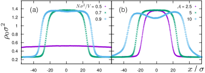
Figure 6: Isotropic Fourier component of the scaled density profile, $\rho_{0}\sigma^{2}$, as a function of $x/\sigma$ obtained from BD simulations for $s\tau/\sigma=60$ and $k_{B}T/\epsilon=0.5$. (a) For different values of the average density $N\sigma^{2}/V=0.5,0.7$, and 0.9 (as indicated) with simulation box aspect ratio ${\cal A}=5$. (b) For different aspect ratios ${\cal A}=2.5,5,$ and 10, with average density $N\sigma^{2}/V=0.7$.

Appendix D Square gradient strength $\xi$

We display in Fig. 7 the Fourier coefficients of the density profile, $\rho_{n}(x)$, for two further values of the strength of the square density gradient term: $\xi=0$ (a), which is identical to omitting the square gradient term in Eq. (38), and as a further representative case $\xi=2100$ (b). As a reference the results for our (optimal) parameter choice $\xi=700$ are also shown (black solid lines); these data are identical to that shown in Fig. 3(a).

It is clear that very large values of $\xi$ introduce artifacts, such as e.g. the double hump in the polarization profile $\rho_{1}$. For very small values of $\xi$ (with zero being an extreme case thereof), the overall amplitudes become exaggerated. The chosen value $\xi=700$ represents a compromise where neither of the two effects is dominant.

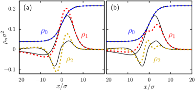
Figure 7: Fourier coefficients $\rho_{n}\sigma^{2}$ of the density distribution as a function of $x/\sigma$ across the interface. Shown are the theoretical results for $n=0,1,2$ (dashed lines, as indicated) for different values of the parameter $\xi=0$ (a) and 2100 (b). As a reference the results for $\xi=700$ are also shown (solid black lines); these results are identical to the data in the right panel of Fig. 3(a).

References

- (1) J. D. van der Waals, On the Continuity of the Gaseous and Liquid States, ed. by J. S. Rowlinson (Dover, New York, 2004).
- (2) J. D. van der Waals, The thermodynamic theory of capillarity under the hypothesis of a continuous variation of density, J. Stat. Phys. 20, 200 (1979) (translation by J. S. Rowlinson); Thermodynamische Theorie der Kapillarität unter Voraussetzung stetiger Dichteänderung, Z. Phys. Chem. 13, 657 (1894) (translation by J. J. van Laar).
- (3) M. von Smoluchowski, Molekular‐kinetische Theorie der Opaleszenz von Gasen im kritischen Zustande, sowie einiger verwandter Erscheinungen, Ann. Phys. 330, 205 (1908).
- (4) L. Mandelstam, Über die Rauhigkeit freier Flüssigkeitsoberflächen, Ann. Phys. 346, 609 (1913).
- (5) J. S. Rowlinson and B. Widom, Molecular Theory of Capillarity (Dover, New York, 2002).
- (6) J. P. Hansen and I. R. McDonald, Theory of Simple Liquids, 4th ed. (Academic Press, London, 2013).
- (7) R. Evans, The nature of the liquid-vapour interface and other topics in the statistical mechanics of non-uniform, classical fluids, Adv. Phys. 28, 143 (1979).
- (8) I. Zhang, R. Pinchaipat, N. B. Wilding, M. A. Faers, P. Bartlett, R. Evans, and C. P. Royall, Composition inversion in mixtures of binary colloids and polymer, J. Chem. Phys. 148, 184902 (2018).
- (9) D. J. Ashton, N. B. Wilding, R. Roth, and R. Evans, Depletion potentials in highly size-asymmetric binary hard-sphere mixtures: Comparison of simulation results with theory, Phys. Rev. E 84, 061136 (2011).
- (10) D. G. Triezenberg and R. Zwanzig, Fluctuation Theory of Surface-Tension, Phys. Rev. Lett. 28, 1183 (1972).
- (11) J. D. Weeks, Structure And Thermodynamics Of Liquid-Vapor Interface, J. Chem. Phys. 67, 3106 (1977).
- (12) M. S. Wertheim, Correlations in liquid-vapor interface, J. Chem. Phys. 65, 2377 (1976).
- (13) A. O. Parry, C. Rascon, and R. Evans, The local structure factor near an interface; beyond extended capillary-wave models, J. Phys.: Condens. Matter 28, 244013 (2016).
- (14) E. Chacón and P. Tarazona, Intrinsic profiles beyond the capillary wave theory: A Monte Carlo study, Phys. Rev. Lett. 91, 166103 (2003).
- (15) D. G. A. L. Aarts, M. Schmidt, and H. N. W. Lekkerkerker, Direct visual observation of thermal capillary waves, Science 304, 847 (2004).
- (16) D. Derks, D. G. A. L. Aarts, D. Bonn, H. N. W. Lekkerkerker, and A. Imhof, Suppression of thermally excited capillary waves by shear flow, Phys. Rev. Lett. 97, 038301 (2006).
- (17) T. H. R. Smith, O. Vasilyev, D. B. Abraham, A. Maciolek, and M. Schmidt, Interfaces in driven Ising models: Shear enhances confinement, Phys. Rev. Lett. 101, 067203 (2008).
- (18) T. F. F. Farage, P. Krinninger, and J. M. Brader, Effective interactions in active Brownian suspensions, Phys. Rev. E 91, 042310 (2015).
- (19) R. Wittmann and J. M. Brader, Active Brownian particles at interfaces: An effective equilibrium approach, EPL 114, 68004 (2016).
- (20) C. Maggi, U. M. B. Marconi, N. Gnan, and R. Di Leonardo, Multidimensional stationary probability distribution for interacting active particles, Sci. Rep. 5, 10742 (2015).
- (21) U. M. B. Marconi and C. Maggi, Towards a statistical mechanical theory of active fluids, Soft Matter 11, 8768 (2015).
- (22) S. Paliwal, J. Rodenburg, R. van Roij, and M. Dijkstra, Chemical potential in active systems: predicting phase equilibrium from bulk equations of state?, New J. Phys. 20, 015003 (2018).
- (23) A. P. Solon, J. Stenhammar, M. E. Cates, Y. Kafri, and J. Tailleur, Generalized thermodynamics of phase equilibria in scalar active matter, Phys. Rev. E 97, 020602(R) (2018).
- (24) A. P. Solon, J. Stenhammar, M. E. Cates, Y. Kafri, and J. Tailleur, Generalized thermodynamics of motility-induced phase separation: phase equilibria, Laplace pressure, and change of ensembles, New J. Phys. 20, 075001 (2018).
- (25) P. Digregorio, D. Levis, A. Suma, L. F. Cugliandolo, G. Gonnella, and I. Pagonabarraga, Full Phase Diagram of Active Brownian Disks: From Melting to Motility-Induced Phase Separation, Phys. Rev. Lett. 121, 098003 (2018).
- (26) V. Prymidis, S. Paliwal, M. Dijkstra, and L. Filion, Vapour-liquid coexistence of an active Lennard-Jones fluid, J. Chem. Phys. 145, 124904 (2016).
- (27) B. van der Meer, V. Prymidis, M. Dijkstra, and L. Filion, Mechanical and chemical equilibrium in mixtures of active spherical particles: Predicting phase behaviour from bulk properties alone, arXiv.org/1609.03867.
- (28) J. Tailleur and M. E. Cates, Statistical mechanics of interacting run-and-tumble bacteria, Phys. Rev. Lett. 100, 218103 (2008); M. E. Cates, Diffusive transport without detailed balance in motile bacteria: does microbiology need statistical physics?, Rep. Prog. Phys. 75, 042601 (2012).
- (29) J. F. Lutsko and J. Lam, Classical density functional theory, unconstrained crystallization, and polymorphic behavior, Phys. Rev. E 98, 012604 (2018); J. F. Lutsko, Systematically extending classical nucleation theory, New J. Phys. 20, 103015 (2018).
- (30) A. Fortini, D. de las Heras, J. M. Brader, and M. Schmidt, Superadiabatic forces in Brownian many-body dynamics, Phys. Rev. Lett. 113, 167801 (2014).
- (31) T. Speck, J. Bialké, A. M. Menzel, and H. Löwen, Effective Cahn-Hilliard Equation, Phys. Rev. Lett. 112, 218304 (2014).
- (32) J. Blaschke, M. Maurer, K. Menon, A. Zöttl, and H. Stark, Phase separation and coexistence of hydrodynamically interacting microswimmers, Soft Matter 12, 9821 (2016).
- (33) S. C. Takatori and J. F. Brady, Towards a thermodynamics of active matter, Phys. Rev. E 91, 032117 (2015).
- (34) J. D. Weeks, D. Chandler, and H. C. Andersen, Role of repulsive forces in determining the equilibrium structure of simple liquids, J. Chem. Phys. 54, 5237 (1971).
- (35) M. Schmidt and J. M. Brader, Power functional theory for Brownian dynamics, J. Chem. Phys. 138, 214101 (2013).
- (36) D. de las Heras, J. Renner, and M. Schmidt, Custom flow in overdamped Brownian Dynamics, Phys. Rev. E 99, 023306 (2019).
- (37) P. Krinninger, M. Schmidt, and J. M. Brader, Nonequilibrium Phase Behavior from Minimization of Free Power Dissipation, Phys. Rev. Lett. 117, 208003 (2016); Erratum 119, 029902 (2017).
- (38) P. Krinninger and M. Schmidt, Power functional theory for active Brownian particles: general formulation and power sum rules, J. Chem. Phys. 150, 074112 (2019).
- (39) For an overview of new developments in classical density functional theory, see: R. Evans, M. Oettel, R. Roth, and G. Kahl, New developments in classical density functional theory, J. Phys.: Condens. Matter 28, 240401 (2016).
- (40) Y. Fily and M. C. Marchetti, Athermal phase separation of self-propelled particles with no alignment, Phys. Rev. Lett. 108, 235702 (2012).
- (41) J. Stenhammar, A. Tiribocchi, R. J. Allen, D. Marenduzzo, and M. E. Cates, Continuum theory of phase separation kinetics for active Brownian particles, Phys. Rev. Lett. 111, 145702 (2013).
- (42) A. P. Solon, J. Stenhammar, R. Wittkowski, M. Kardar, Y. Kafri, M. E. Cates, and J. Tailleur, Pressure and phase equilibria in interacting active Brownian spheres, Phys. Rev. Lett. 114, 198301 (2015).
- (43) Going beyond this approximation requires to introduce two further superadiabatic force density fields, and . These contribute to the total internal force density, such that . The additional fields are kinematic functionals and are specfified by the cancellations and . Then in the correlator expressions (32), (34), (41) and (45) the full internal force density field needs to be replaced by .
- (44) The density distribution in a standard DFT of spheres with no orientations is given by .
- (45) A. Santos, M. López der Haro, and S. Bravo Yuste, An accurate and simple equation of state for hard disks, J. Chem. Phys. 103, 4622 (1995).
- (46) J. T. Siebert, F. Dittrich, F. Schmid, K. Binder, T. Speck, and P. Virnau, Critical behavior of active Brownian particles, Phys. Rev. E 98, 030601 (2018).
- (47) The polynomial is where and indicates the critical packing fraction.
- (48) S. Paliwal, V. Prymidis, L. Filion, and M. Dijkstra, Non-equilibrium surface tension of the vapour-liquid interface of active Lennard-Jones particles, J. Chem. Phys. 147, 084902 (2017).
- (49) This form implies that the -axis points towards the dense phase, as is the case in the present setup.
- (50) S. C. Takatori, W. Yan, and J. F. Brady, Swim pressure: stress generation in active matter, Phys. Rev. Lett. 113, 028103 (2014).
- (51) X. B. Yang, L. M. Manning, and M. C. Marchetti, Aggregation and segregation of confined active particles, Soft Matter 10, 6477 (2014).
- (52) D. de las Heras and M. Schmidt, Velocity gradient power functional for Brownian dynamics, Phys. Rev. Lett. 120, 028001 (2018).
- (53) N. C. X. Stuhlmüller, T. Eckert, D. de las Heras and M. Schmidt, Structural nonequilibrium forces in driven colloidal systems, Phys. Rev. Lett. 121, 098002 (2018).
- (54) J. Guioth and E. Bertin, Large deviations and chemical potential in bulk-driven systems in contact, EPL 123, 10002 (2018).
- (55) R. Dickman and R. Motai, Inconsistencies in steady-state thermodynamics, Phys. Rev. E 89, 032134 (2014).
- (56) R. Dickman, Phase coexistence far from equilibrium, New J. Phys. 18, 043034 (2016).
- (57) E. Bertin, Theoretical approaches to the steady-state statistical physics of interacting dissipative units, J. Phys. A: Math. Theor. 50, 083001 (2017).
- (58) J. Guioth and E. Bertin, Lack of an equation of state for the nonequilibrium chemical potential of gases of active particles in contact, J. Chem. Phys. 150, 094108 (2019).
- (59) T. Speck, Stochastic thermodynamics for active matter, EPL 114, 30006 (2016).
- (60) J. Bialké, J. T. Siebert, H. Löwen, T. Speck, Negative Interfacial Tension in Phase-Separated Active Brownian Particles, Phys. Rev. Lett. 115, 098301 (2015).
- (61) S. Hermann, D. de las Heras, M. Schmidt (to be published).
- (62) C. F. Lee, Interface stability, interface fluctuations, and the Gibbs-Thomson relationship in motility-induced phase separations, Soft Matter 13, 376 (2017).
- (63) A. Patch, D. M. Sussman, D. Yllanes, and M. C. Marchetti, Curvature-dependent tension and tangential flows at the interface of motility-induced phases, Soft Matter 14, 7435 (2018).
- (64) J. Dzubiella, H. Löwen, and C. N. Likos, Depletion forces in nonequilibrium, Phys. Rev. Lett. 91, 248301 (2003).
- (65) A. Patch, D. Yllanes, M. C. Marchetti, Kinetics of motility-induced phase separation and swim pressure, Phys. Rev. E 95, 012601 (2017).