Particle acceleration in interstellar shocks

Abstract

This review presents the fundamentals of the particle acceleration processes active in interstellar medium (ISM), which are essentially based on the so-called Fermi mechanism theory. More specifically, the review presents here in more details the first order Fermi acceleration process – also known as diffusive shock acceleration (DSA) mechanism. In this case, acceleration is induced by the interstellar (IS) shock waves. These IS shocks are mainly associated with emission nebulae (H ii regions, planetary nebulae and supernova remnants). Among all types of emission nebulae, the strongest shocks are associated with supernova remnants (SNRs). Due to this fact they also provide the most efficient manner to accelerate ISM particles to become high energy particles, i.e. cosmic-rays (CRs). The review therefore focuses on the particle acceleration at the strong shock waves of supernova remnants.

1 Introduction

Enrico Fermi suggested in his seminal paper (Fermi 1949) an elegant way of acceleration of charged particles to the energies of most Galactic cosmic-rays. He derived that the energy gain in a collision between a particle and the magnetic field perturbation is $\propto(u/c)^{2}$. Here $u$ represents the speed of the magnetic field perturbation, and $c$ the speed of high-energy particle. In the interstellar conditions, the acceleration process suggested by Fermi is actually not very efficient, as $u/c$ is already a small value quantity, for non-relativistic shocks, which is then squared. On the other hand, the fact that particles can gain energy in collisions with the moving magnetic field irregularities (so-called magnetic mirrors) served as a fundamental starting point for all later acceleration theories seeking to explain CR creation in ISM. Approximately three decades later, this original mechanism of particle acceleration became known as the so-called second order Fermi acceleration mechanism, because a new theory started developing – the first order Fermi acceleration or diffusive shock acceleration theory. Actually, in DSA acceleration model, the gain of particle energy through repeated shock crossings by successive head-on interaction with up and downstream disturbances, is $\propto u/c$ (e.g. Bell 1978a). In that sense, shock waves in ISM transform part of the bulk kinetic energy into thermal energy, but also in the CR acceleration.

As we will see, collisionless shock waves are crucial phenomena for particle acceleration in ISM. The formation of such a shock wave in magnetized IS plasma, the charged particle acceleration and the magnetic field amplification are coupled processes. We can simply say that, on microscopic level, a shock is formed when the charged particles are reflected by an electromagnetic barrier. The ordinary collisions between particles are not frequent enough as in ordinary hydrodynamical shocks (actual dissipation cannot be established by a simple particle-particle interaction). However, we note that various processes, like resonant microinstabilities, which actually trigger colissionless shock-formation and evolution are still not fully understood (see e.g. Zeković 2019). The various shock waves in ISM are mainly associated with the known emission nebulae. There are generally three basic types of emission nebulae: H ii regions, planetary nebulae (PNe) and supernova remnants (SNRs). In H ii regions around young, massive and hot stars, the existence of shocks can be expected in weak (isothermal, radiative) form. Even though PNe are essentially H ii regions, they have two associated shock waves: inner one which is strong (adiabatic, non-radiative), and outer one which is weak (isothermal or radiative shock). Supernova remnants in the first two phases of evolution (free expansion and Sedov phases) have strong, non-radiative shock waves. In the third, isothermal phase of evolution, these previously strong shock waves rapidly lose kinetic energy and become weaker, radiative shocks. We expect particle acceleration at all kinds of collisionless shocks, strong or weak, but efficient acceleration should be expected only at strong shocks of supernova remnants. In addition, the inferred Galactic cosmic-ray energy density (order of $1\ \mathrm{eV}\ \mathrm{cm^{-3}}$), combined with the estimated time of the average CR existence in our galaxy, requires a Galactic CR production with a total power of about $10^{41}\ \mathrm{erg}\ \mathrm{s^{-1}}$ (Ginzburg & Syrovatskij 1967). With the mean supernova (SN) explosion energy of around $10^{51}\ \mathrm{erg}$ and an inferred Galactic SN rate of several events per century, SNe and their remnants are the most probable sources known to be able to provide such a power. The inner shocks of PNe are strong, but corresponding shock speeds are significantly lower than those of young SNRs. Additionally PNe are short living objects with significantly lower energy contents. However, we can expect particle acceleration in PN shocks, but at this moment we do not have observational evidence for creation of high energy particles in PNe – this can be the subject of future research.

In this review, we present the details of DSA theory. In fact, we start with the basic particle acceleration model given by famous Enrico Fermi (Section 2.1), and then continue with the elaboration of the so-called microscopic and macroscopic approaches to the test-particle DSA mechanism (Sections 2.2 and 2.3). In addition, we discuss the consequences of the CR back-reaction through the non-linear DSA (Section 2.4). Finally, we emphasize the most important observational signatures which confirm DSA mechanism in SNRs (Section 3).

2 Fermi acceleration

2.1 The original Fermi approach

In this subsection we present the original Fermi (1949) approach. Let us assume a moving magnetic perturbation of ISM (e.g. a magnetized cloud) along the $x$-axis, moving with speed $u$ in the fixed reference frame of the observer. Let us also consider a particle with speed $v$ also in the reference frame of observer; $u$ and $v$ are speeds of a moving magnetic perturbation and a particle, respectively, before collision. In the beginning, we consider the case where the test-particle moves in a direction opposite to the motion of magnetized cloud, and has initial energy $\mathcal{E}=mc^{2}+E$, where $\mathcal{E}$ is the total energy, $m$ is the particle rest mass, $c$ is the speed of light, and $E$ is the particle kinetic energy. We assume that particle is gyrating in a low-density medium with a turbulent magnetic field. When it collides with the cloud, a charged particle is reflected by the so-called magnetic mirror and comes back with the same pitch angle $\theta$ and the direction of motion of its guiding center being inverted. Applying the relativistic transformations between a ’laboratory’ (observer’s) reference frame at rest and the moving (primed) reference frame of the cloud, the energy and the momentum of the particle before collision are respectively:

$$\mathcal{E}^{\prime}=\gamma_{u}(\mathcal{E}+up_{x}),\quad p_{x}^{\prime}=\gamma_{u}(p_{x}+u\mathcal{E}/c^{2}),\qquad\gamma_{u}=1/{\sqrt{1-u^{2}/c^{2}}}.$$ (1)

The collision between particle and a magnetized cloud is elastic, and in ’primed’ reference frame the total energy of the test charged particle does not change after collision $(\mathcal{E}^{\prime}_{\rm before\,coll.}=\mathcal{E}^{\prime}_{\rm after\,coll.})$. Also, the intensity of the particle momentum stays constant after collision in ’primed’ reference frame, but with opposite sign, i.e. $p_{x}^{\prime}$ will be transformed to $-p_{x}^{\prime}$ after collision. We can move back to the observer’s reference frame by using similar reasoning, as $u$ and $v$ vectors are oriented in the same direction after collision ($\mathcal{E}^{\prime}=\gamma_{u}(\mathcal{E}-up_{x}),\,p_{x}^{\prime}=\gamma_{u}(u\mathcal{E}/c^{2}-p_{x})$). We change $p_{x}^{\prime}$ into $-p_{x}^{\prime}$ to account for the inversion of the direction of propagation of the particle, and obtain:

$$\mathcal{E_{\rm after\,coll.}}=\gamma_{u}(\mathcal{E}^{\prime}+up_{x}^{\prime})=\gamma_{u}^{2}(\mathcal{E}+2up_{x}+u^{2}\mathcal{E}/c^{2}),$$ (2)

i.e., since (by using $p=\gamma mv$ and $\mathcal{E}=\gamma mc^{2}$), $p_{x}/\mathcal{E}=p{\cos}\theta/\mathcal{E}=v\cos\theta/c^{2}$,

$$\frac{\mathcal{E_{\rm after\,coll.}}}{\mathcal{E}}=\frac{1+2(u/c)(v/c)\cos\theta+(u/c)^{2}}{1-(u/c)^{2}}\approx 1+2(u/c)(v/c)\cos\theta+2(u/c)^{2}.$$ (3)

The resulting expression in Eq. (3) is obtained under particular approximation $(1-(u/c)^{2})^{-1}\approx 1+(u/c)^{2}$ and by neglecting all terms in which $u/c$ appears with the power $\geq 3$.

The probabilities of head-on and head-tail collisions are proportional to the intensity of relative velocities of approach of the particle and the cloud, i.e. $v+u\cos\theta$ and $v-u\cos\theta$ in the direction of the test-particle trajectory, respectively (for $\cos\theta>0$). Assuming high energy test-particle, for $v\approx c$ and $0<\theta<\pi$ we can write this probability as proportional to $1+(u/c)\cos\theta$, and average the second term in Eq. (3) to obtain (Longair 2011):

$$\left\langle\frac{2u}{c}\cos\theta\right\rangle=\frac{2u}{c}\frac{\int_{-1}^{1}\mu(1+(u/c)\mu)d\mu}{\int_{-1}^{1}(1+(u/c)\mu)d\mu}=\frac{2}{3}\Big{(}\frac{u}{c}\Big{)}^{2},\ \ \ \mu=\cos\theta,$$ (4)

i.e.

$$\langle{\Delta E}/{E}\rangle=\frac{8}{3}\Big{(}\frac{u}{c}\Big{)}^{2},$$ (5)

where we present the expression for the particle kinetic energy $E$ increment, under assumption of negligible rest energy in comparison to total energy of accelerated particles.

Under the starting assumption that a high energy test-particle has the same direction as a moving magnetic perturbation (head-tail, rear-on or overtaking collision), transformations between ’primed’ and observer’s reference frames for the total energy and momentum of the particle are inverted (with respect to the cases before and after collision). In the case before collision for the transformation into the ’primed’ frame we use $\mathcal{E}^{\prime}=\gamma_{u}(\mathcal{E}-up_{x}),\,p_{x}^{\prime}=\gamma_{u}(u\mathcal{E}/c^{2}-p_{x})$. In the case after collision for the return into the observer’s reference frame, we have:

$$\mathcal{E_{\rm after\,coll.}}=\gamma_{u}(\mathcal{E}^{\prime}+up_{x}^{\prime})=\gamma_{u}^{2}(\mathcal{E}-2up_{x}+u^{2}\mathcal{E}/c^{2}),$$ (6)

Due to this, the analogue expression to Eq. (3), for the case of overtaking collision is:

$$\frac{\mathcal{E_{\rm after\,coll.}}}{\mathcal{E}}\approx 1-2(u/c)(v/c)\cos\theta+2(u/c)^{2},$$ (7)

which after the same procedure applied previously for head-on collision and assuming that the probability of head-tail collision is proportional to $1-(u/c)\cos\theta$ gives again $\langle{\Delta E}/{E}\rangle=8/3(u/c)^{2}$.

As we can see from previously given equations, in the original version of the Fermi acceleration theory (Fermi 1949) $+$ and $-$ signs in front of the linear term $(u/c)$ correspond, respectively, to the head-on (approaching) or head-tail (receding) motion of the magnetic mirror, and hence to a gain or a loss of energy. As a result, this linear term disappears from the corresponding equations. Since the direct collisions (head-on) are statistically more numerous than the overtaking ones (for the same reason that car windscreens get wetter than rear windows), there is a net energy gain for the charged particle, whose energy increases continuously due to the numerous accumulated collisions, and this gain is represented by the second order dependence $(u/c)^{2}$ that survived in Eq. (5).

2.2 DSA - microscopic approach

In the interstellar conditions, the original mechanism proposed by Enrico Fermi is not very efficient and we should try to establish a model in which only head-on collisions exist. It means that the linear term $u/c$ (Eqs. 3 and 7) does not vanish. A modern version of the first order Fermi acceleration (DSA theory) was developed independently by Axford et al. (1977), Krymsky (1977), Bell (1978a) and Blandford & Ostriker (1978). There were two approaches to the problem: macroscopic (e.g. Blandford & Ostriker 1978) and microscopic (Bell 1978a). In the rest of this subsection we will follow the derivation by Bell (1978a).

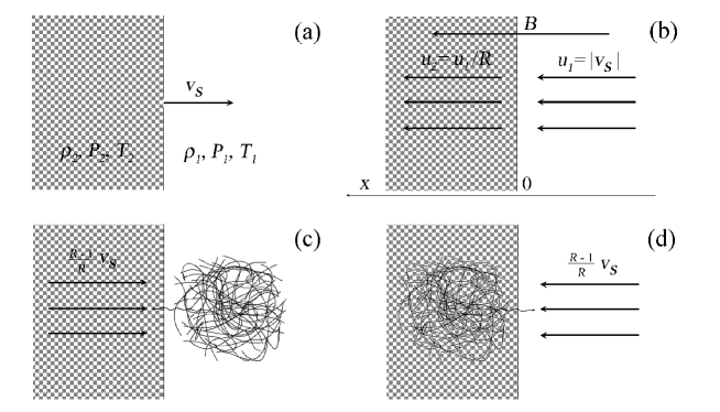
Figure 1: Diffuse shock acceleration of high energy particles in the vicinity of a strong shock wave. Adapted from Longair (2011).

Let us start with consideration of a strong shock wave moving through the surrounding medium with speed $v_{\rm s}$ in the observer’s (rest) frame (Fig. 1a). In the moving frame which is connected to the shock (Fig. 1b), the upstream gas flows through the shock front with speed $u_{1}=|v_{\rm s}|$. We assume that the shock surface is orthogonal to the magnetic field lines $B$ (i.e. parallel MHD shock wave). The equation of continuity (mass conservation) requires $\rho_{1}u_{1}=\rho_{2}u_{2}$ and the so-called Rankine-Hugoniot relations give us $\rho_{2}/\rho_{1}=u_{1}/u_{2}=R=(\gamma+1)/(\gamma-1)$, where $\gamma$ is the ratio of specific heats of the gas. The compression ratio $R$ equals $4$ in the case of the strongest shocks.

Let us assume the existence of high-energy particles in the upstream region (ahead of the shock front) whose distribution function is isotropic in the frame of reference in which the gas is at rest (Fig. 1c). This reference frame is equivalent to the observer’s (rest) frame. These so-called test-particles cross the shock front and so encounter gas behind the shock traveling at the speed $3/4v_{\rm s}$ if the shock is very strong. They are scattered by the magnetic irregularities in the downstream region (behind the shock front) and they receive a small amount of energy $\Delta E/E\sim v_{\rm s}/c$. Their distribution function is also isotropized – their velocity distribution is now isotropic in the reference frame in which the downstream gas is at rest, and they are ready to move back to the upstream region. Now, we consider the opposite process when high-energy test-particle recross the shock front, from the downstream to the upstream region (Fig. 1d). Due to that, when test particles cross the shock front from downstream to upstream, they encounter the upstream gas moving at speed $3/4v_{\rm{\rm s}}$ and are again able to receive a small amount of energy. Actually, in the upstream region they are scattered back by the Alfvén waves excited by the energetic particles themselves, as they move at super-Alfvénic velocities and attempt to escape from the shock. As a result, particles can recross the shock front again. In each shock recrossing, after collisions with downstream and upstream magnetic mirrors, they receive a small amount of energy – there are no collisions in which a particle loses energy.

After this more qualitative explanation, we move on to a more detailed theory of DSA (see Bell 1978a, Lequeux 2005, Longair 2011, Arbutina 2017). We consider the existence of test-particles and introduce their so-called phase-space distribution function, in particular its isotropic part $f(x,p,t)$. These charged particles are injected into the planar, one-dimensional MHD shock, parallel or nearly parallel (with shock velocity directed along the $x$-axis practically aligned with mean (galactic) magnetic field) with speed much higher than that of the shock, $v\gg v_{\rm s}$. In these collisionless shocks, the average, homogeneous magnetic field plays essentially no role, while fluctuations in that average field play an important role as scattering centers in the downstream region. In fact, we consider collisionless shock waves as ordinary hydrodynamic shocks that propagate through the homogeneous magnetized plasma, as well as additional scattering centers. We choose a reference frame in which the shock is stationary (Fig. 1b). The gas flows from upstream, $(x<0)$ with speed $u_{1}=|v_{\rm s}|$, to downstream where $u_{2}<|v_{\rm s}|$. In that sense, we are dealing with diffusion in a fluid moving with different velocities on either side of the shock. Diffusion in a fluid is introduced by diffusion-advection equation near a discontinuity (Drury 1983, Blandford & Eichler 1987), which represents general kinetic equation for cosmic-rays (Skilling 1971, 1975), sometimes called Parker’s transport equation because it was derived for the first time in Parker (1965):

$$\frac{\partial{f}}{\partial{t}}+u\frac{\partial{f}}{\partial{x}}=\frac{\partial}{\partial{x}}{\bigg{[}}D(x,p)\frac{\partial{f}}{\partial{x}}{\bigg{]}}+\frac{1}{3}\frac{\partial{u}}{\partial{x}}p\frac{\partial{f}}{\partial{p}}+Q(x,p),$$ (8)

where

$$D(x,p)=\frac{\lambda v}{3}$$ (9)

is the diffusion coefficient in the $x$ direction for particles with speed $v$. The mean free path of particles ($\lambda$) is assumed to be $\lambda{\sim}r_{g}$,

$$r_{\rm g}=\frac{p_{\perp}}{eB}\frac{A}{Z},$$ (10)

where $r_{\rm g}$ is the gyro-radius of charged particle with the atomic mass number $A$, the charge number $Z$ in the magnetic field $B$. Here the elementary charge is given by the symbol $e$ and the perpendicular component of momentum $p_{\perp}$. The last term in Eq. (8) describes injection and we assume $\delta$-function for injection at the shock.

Equations (9) and (10) actually assume standard isotropic Bohm diffusion. It is important to note that the Bohm limit for the parallel diffusion coefficient was derived in Shalchi (2009) and tested numerically by Hussein & Shalchi (2014).

Under the assumption of stationarity we have ${\partial{f}}/{\partial{t}}=0$ and ${\partial{u}}/{\partial{t}}=0$ outside the shock. Additionally we assume constant downstream velocity (${\partial{u}}/{\partial{x}}=0$). Due to these simplifications, the diffusion-advection equation for particles which enter the downstream region (Eq. (8)) becomes:

$$u_{2}\frac{\partial{f}}{\partial{x}}-\frac{\partial}{\partial{x}}\left[D(x,p)\frac{\partial{f}}{\partial{x}}\right]=0.$$ (11)

The general solution of this partial differential equation, obtained by double integration over $x$, is:

$$f(x,p)=A(p)+B(p)\exp\left(\int{\frac{u_{2}}{D(x^{\prime},p)}dx^{\prime}}\right),$$ (12)

where $A$ and $B$ are the integration constants. The diffusion coefficient $D(x^{\prime},p)$ takes finite values, while $x$ extends to infinity. Due to this the second term diverges, unless $B=0$. A physical solution therefore requires that $f(x,p)=A(p)$ i.e. it is a function of momentum only. The flow of particles far away from the shock into the downstream region, i.e. the current density of particles that escape from the shock far downstream is $u_{2}n(x,p)-D(x,p)(\partial{n}/\partial{x})$, which is equal to $u_{2}n(0,p)$, where the number density of particles $n=\int_{0}^{\infty}4\pi p^{2}f(p)dp$, is defined for isotropic distribution. The flux density, i.e. the rate at which particles are crossing and recrossing the shock is:

$$\int\int fv_{x}p^{\prime 2}dp^{\prime}d\Omega =\int_{0}^{\infty}2\pi v(p^{\prime})f(p^{\prime})p^{\prime 2}dp^{\prime}\int_{0}^{\pi/2}\cos\theta\sin\theta d\theta=$$ (14)

$$=\frac{1}{2}vn\int_{0}^{1}\mu d\mu=\frac{1}{4}vn(0,p),$$

where $d\Omega$ is the elementary solid angle, $\mu=\cos\theta$ and we assume $f(p^{\prime})=\frac{n}{4\pi p^{2}}\delta(p-p^{\prime})$. We use the well-known behavior of the $\delta$-function $f(x)=\int f(x^{\prime})\delta(x^{\prime}-x)dx^{\prime}$. Finally, we obtain the escape probability in the form:

$$\eta=\frac{u_{2}n(0,p)}{\frac{1}{4}vn(0,p)}=4\frac{u_{2}}{v}.$$ (15)

For relativistic particles ($v\approx c$) and non-relativistic shock waves, this probability is rather low.

Now we focus to the reference frames in which DSA mechanism can be analytically described. We can define a rest frame attached to the magnetic mirror which is in the downstream region of a shock wave. This magnetic mirror has velocity $u_{1}-u_{2}$ relative to the reference frame of upstream isotropically distributed particles (see Fig. 1c). On the other hand, in the upstream region we can define another magnetic mirror with the same velocity $u_{1}-u_{2}$ (this is velocity in the reference frame connected to downstream isotropically distributed particles (Fig. 1d)). The upstream magnetic mirror is at rest in the upstream fluid (observer’s) reference frame. Due to this we define another rest reference frame to the upstream magnetic mirror. These two rest reference frames tied to both magnetic mirrors are necessary for the next derivation. When a test-particle with injection energy $E_{0}$ in the fixed, upstream fluid (observer’s) reference frame goes from upstream (region 1) to downstream (region 2), its energy (according to Eq. (2), ${E}^{\prime}=\gamma_{u}({E}+up_{x})$) is:

$$E_{1}^{\rm down.\,mirror}\approx E_{0}{\bigg{[}}1+(u_{1}-u_{2})\frac{v_{11}\cos{\theta_{11}}}{c^{2}}{\bigg{]}},$$ (16)

with $\gamma_{u}\approx 1$ (because of $(u_{1}-u_{2})^{2}/c^{2}\ll 1$) for non-relativistic shocks; here $E_{1}^{\rm down.\,mirror}$ represents the test-particle energy in the rest reference frame of downstream magnetic mirror. When the same particle comes back to region 1, its energy in the rest frame of the upstream magnetic mirror is:

$$\frac{E_{1}^{\rm up.\,mirror}}{E_{0}}\approx{\bigg{[}}1+(u_{1}-u_{2})\frac{v_{11}\cos{\theta_{11}}}{c^{2}}{\bigg{]}}{\bigg{[}}1+(u_{1}-u_{2})\frac{v_{12}\cos{\theta_{12}}}{c^{2}}{\bigg{]}}.$$ (17)

where first index in $v$ and $\theta$ denotes cycle number, while second index denotes passing from region 1 to region 2 (index 1) and from region 2 to region 1 (index 2). Eq. (17) represents a starting expression for the acceleration of test-particle by the DSA mechanism and it is analogue to Eq. (3). Here, $v_{12}$ and $\theta_{12}$ are assumed to be in the upstream mirror reference frame as it is presented by Bell (1978a) – we do not use these quantities in the downstream mirror reference frame (as in Lequeux 2005). For averaging per angle $\theta$, the necessary condition is that angles $\theta_{11}$ and $\theta_{12}$ should be expressed in the same reference frame (we chose it to be the upstream mirror frame). Eq. (17) has different form in Bell (1978a) – the reason for that is opposite direction of measuring $\theta$. We assume here the direction as given in Lequeux (2005). The sign $\approx$ instead equality in Eq. (17) is a result of transformation from the downstream to the upstream mirror frame ($p_{x}^{\rm up.\,mirror}=\gamma_{u_{1}-u_{2}}(p_{x}^{\rm down.\,mirror}+(u_{1}-u_{2})E_{1}^{\rm down.\,mirror}/c^{2}$), and by using approximation $\gamma_{u_{1}-u_{2}}=(1-((u_{1}-u_{2})/c)^{2})^{-1/2}\approx 1+1/2((u_{1}-u_{2})/c)^{2}$, where finally we have term $v_{12}\cos\theta_{12}/c^{2}$.

We emphasize again that our test-particle is already highly energized ($v\approx c$) at the injection. Due to this, by using $v_{k1}/c\approx 1$ and $v_{k2}/c\approx 1$ which provide that the test-particle gets the same portion of energy in every interaction with magnetic mirrors, the energy of test-particle after $l$ cycles is:

$$\frac{E_{l}}{E_{0}}=\prod_{k=1}^{l}{\frac{E_{k}^{\rm up.\,mirror}}{E_{0}}}=\left(\frac{E_{1}^{\rm up.\,mirror}}{E_{0}}\right)^{l},$$ (18)

where

$${\frac{E_{k}^{\rm up.\,mirror}}{E_{0}}}=\frac{1}{E_{0}}{\bigg{[}}1+(u_{1}-u_{2})\frac{\cos{\theta_{k1}}}{c}{\bigg{]}}{\bigg{[}}1+(u_{1}-u_{2})\frac{\cos{\theta_{k2}}}{c}{\bigg{]}},$$ (19)

i.e.

$$\ln\left({\frac{E_{l}}{E_{0}}}\right)=l\ln\left(\frac{E_{1}^{\rm up.\,mirror}}{E_{0}}\right).$$ (20)

For a significant energy increase, $l$ must be at least of the order of $c/(u_{1}-u_{2})$. The distribution of $\ln({{E_{l}}/{E_{0}}})$ will be strongly concentrated around the mean, so we can treat all particles completing $l$ cycles as having their energy increased by the same amount, and by using Eq. (19) with ${\frac{E_{k}^{\rm up.\,mirror}}{E_{0}}}=\frac{E_{1}^{\rm up.\,mirror}}{E_{0}}$, we obtain:

$$\ln\left(\frac{E_{l}}{E_{0}}\right)=l\Big{[}\Big{\langle}\ln\big{(}1+\frac{u_{1}-u_{2}}{c}\cos\theta_{k1}\big{)}\Big{\rangle}+\Big{\langle}\ln\big{(}1+\frac{u_{1}-u_{2}}{c}\cos\theta_{k2}\big{)}\Big{\rangle}\Big{]}.$$ (21)

After the expansion of logarithm function in power series we find:

$$\ln\left(\frac{E_{l}}{E_{0}}\right)\approx l\frac{u_{1}-u_{2}}{c}\left[\langle\cos\theta_{k1}\rangle+\langle\cos\theta_{k2}\rangle\right].$$ (22)

The number of particles that cross the shock between angles $\theta$ and $\theta+d\theta$ is proportional to $2\pi{\sin\theta}{\cos\theta}d\theta$. After averaging over angles from 0 to $\pi/2$ we have:

$$\langle\cos\theta_{k1}\rangle=\langle\cos\theta_{k2}\rangle=\frac{\int_{0}^{1}\mu^{2}d\mu}{\int_{0}^{1}\mu d\mu}=\frac{2}{3}.$$ (23)

Finally,

$$\ln\left(\frac{E_{l}}{E_{0}}\right)=\frac{4}{3}l\frac{u_{1}-u_{2}}{c}.$$ (24)

The probability of completing at least $l$ cycles and reaching energy $E\geq E_{l}$ is given by:

$${P}_{l}=\frac{N(E\geq E_{l})}{N_{o}}=\zeta^{l},\ \ \ \zeta=1-\eta,$$ (25)

where $\zeta$ is the probability of staying in the acceleration process after one cycle and $N_{0}$ is the initial number of particles. Each particle has the same energy $E_{0}$ at the injection. The number of particles that reached $E\geq E_{l}$ is designated by $N(E\geq E_{l})$. Using Eqs. (15) and (25) leads to:

$$\ln{P}_{l}=l\ln\Big{(}1-\frac{4u_{2}}{c}\Big{)}\approx-l\frac{4u_{2}}{c}=-\frac{3u_{2}}{u_{1}-u_{2}}\ln\left(\frac{E_{l}}{E_{0}}\right).$$ (26)

By combining Eqs. (24) and (26) we have:

$${N(E\geq E_{l})}={N_{o}}\left(\frac{E_{l}}{E_{0}}\right)^{1-\mathnormal{\Gamma}}=\int_{E_{l}}^{\infty}N(E)dE,\ \ \ \mathnormal{\Gamma}=\frac{R+2}{R-1},\ \ \ R=\frac{u_{1}}{u_{2}}.$$ (27)

At the end, the differential particle energy spectrum has a form:

$${N(E)}=KE^{-\mathnormal{\Gamma}},$$ (28)

where $K$ is constant. In the case of strong shocks, the compression $R=4$, so the energy index $\mathnormal{\Gamma}=2$. We emphasize here that Eq. (28) is derived by using the assumption that approximately all $N_{0}$ particles at the beginning of the acceleration process become cosmic-rays. It means that all of them reach energy $E_{l}$. The main reason for the validity of this assumption is based on the starting assumption that all $N_{0}$ particles are highly energized at the injection i.e. $v/c\approx 1$, which provides $\zeta\approx 1$. Due to this, in the limiting situation the integration in Eq. (27) can be from $E_{0}$ to $\infty$.

As a summary of the microscopic approach of test-particle DSA presented in this subsection, we emphasize that the net energy gain in the acceleration process is substantially higher if there are only direct (head-on) collisions. It provides that energy increase is $\Delta E/E\propto(u_{1}-u_{2})/c$ in each collision. As we mentioned earlier, the microscopic DSA model is based on multiple transition of one charged particle through the shock discontinuity from upstream to downstream region and vice-versa. In every passage (head-on) across the shock, independent from which side of the shock the passage occurs, the test-particle gains energy. Owing to this DSA is a more efficient process than original Fermi 2 mechanism (Eq. (5)), where the overtaken collisions exist. If an astrophysical source is linked to a shock wave, we can generally expect acceleration of charged particles from the medium around the shock. Particles such as protons and other heavier ions can be accelerated very efficiently to $\sim 10^{15}$ eV by DSA process (see e.g. Bell et al. 2013 and references therein). Of course, electrons can also be accelerated to the ultra-relativistic energies ($\sim 10^{12}$ eV) at the strong shocks of SNRs, but will suffer more significant energy losses (see e.g. Blasi 2010). Once again, we emphasize that the basic assumption of this derivation is that before the actual start of DSA mechanism the particle has very high velocity $v\gg u$. Finally, this theory predicts a power-law energy spectrum of accelerated particles (Eq. (28)). As we showed here, this theory also predicts a value of $\mathnormal{\Gamma}=2$ for accelerated particles at the strong shock waves with the compression ratio $R=u_{1}/u_{2}=4$. DSA model can be generalized to include lower starting velocities of test-particles (Bell 1978b, see also Section 2.3.2 in Arbutina 2017) which will result in a power-law in momentum:

$$N(p)\propto p^{-\mathnormal{\Gamma}}.$$ (29)

Of course, in any case the initial velocity of the particles must be larger than that of the shock, i.e. the particles must be supra-thermal. Another interesting process is the re-acceleration of CRs which is most commonly assumed to be a diffusive process in which Galactic CRs are re-accelerated through the second order Fermi process in the ISM (e.g. Drury & Strong 2015). However, one can consider the re-acceleration of pre-existing CRs by the shock through DSA mechanism. In this case the pre-existing CRs are actually seed particles that are injected in DSA process (e.g. see Section 2.3.4 in Arbutina 2017). Furthermore, Caprioli et al. (2018) have shown that the cosmic-ray particles can be effectively reflected and accelerated regardless of the shock inclination via the so-called diffusive shock re-acceleration mechanism. They concluded that re-accelerated high-energy particles can drive the streaming instability in the shock upstream and produce effective magnetic field amplification. In that case, the injection of thermal particles can be triggered even at quasi-perpendicular IS shocks. Finally, it is also possible to account for the CR back-reaction and to discuss how the non-linear effects influence simple DSA theory presented here (e.g. Drury 1983, Malkov & Drury 2001; see also Section 2.4 of this review).

2.3 DSA - macroscopic approach

Macroscopic approach to DSA was developed independently by Axford et al. (1977), Krymsky (1977) and Blandford & Ostriker (1978) by considering diffusion-advection equation for CRs. To derive this equation one should start from collisionless plasma kinetic equation in the following suitable form:

$$\frac{\partial f}{\partial t}+\frac{\partial}{\partial\mathbf{x}}\cdot\Big{(}f\mathbf{v}\Big{)}+\frac{\partial}{\partial\mathbf{p}}\cdot\Big{(}f\frac{d\mathbf{p}}{dt}\Big{)}=0,$$ (30)

transform it to a non-inertial wave frame and average over gyration phase to obtain (see Skilling 1971 and Blandford & Eichler 1987 for more details):

$$\Big{(}1+\frac{\mathbf{v\cdot w}}{c^{2}}\Big{)}\frac{\partial f}{\partial t}+(\mathbf{v}+\mathbf{w})\cdot\nabla f-m\gamma\Big{(}\frac{\partial\mathbf{w}}{\partial t}+\mathbf{v}\cdot\nabla\mathbf{w}\Big{)}\cdot\frac{\partial f}{\partial\mathbf{p}} \approx$$

$$\frac{\partial f}{\partial t}+(\mu v\mathbf{n}+\mathbf{u})\cdot\nabla f-\Big{(}\frac{1-\mu^{2}}{2}\nabla\cdot\mathbf{u}+\frac{3\mu^{2}-1}{2}(\mathbf{n}\cdot\nabla)(\mathbf{n}\cdot\mathbf{u})\Big{)}p\frac{\partial f}{\partial{p}} +$$

$$\frac{1-\mu^{2}}{2}\Big{(}{v}\nabla\cdot\mathbf{n}+\mu\nabla\cdot\mathbf{u}-3\mu(\mathbf{n}\cdot\nabla)(\mathbf{n}\cdot\mathbf{u})\Big{)}\frac{\partial f}{\partial{\mu}} =$$

$$\frac{\partial}{\partial\mu}\Big{(}\frac{1-\mu^{2}}{2}\nu_{\rm c}\frac{\partial f}{\partial\mu}\Big{)}$$ . (31)

In the last equation, after a transformation $\mathbf{v}\rightarrow\mathbf{v}+\mathbf{w}\approx\mathbf{v}+\mathbf{u}$, distribution function $f$ and momentum $\mathbf{p}$ are measured in the wave frame, while the coordinates $\mathbf{x}$ are still measured in the inertial frame. The wave frame in which CR particles (mainly protons) scatter elastically of, presumably, Alfvén waves, has the velocity with respect to the inertial frame $\mathbf{w}=\mathbf{u}+v_{\mathrm{A}}\mathbf{n}\approx\mathbf{u}$, where ${u}\ll c$ is the speed of the background plasma, $v_{\mathrm{A}}$ is the Alfvén speed and $\mathbf{n}$ the unit vector along the local magnetic field. A consequence of the transformation is that there is now a collisional, diffusion term on the right-hand side of Eq. (31) due to waves scattering, but because of the energy conservation, the scattering is only in the pitch angle ($\mu$ is the cosine of the pitch angle), with $\nu_{\rm c}$ representing collision frequency, related to the scattering of particles in pitch angle by hydromagnetic waves – ’collective interactions’, occurring through fluctuating electric and magnetic fields.

The last term of Eq. (31) is the so-called pitch-angle scattering term in the isotropic form. This is the usual assumption that actually means that the pitch-angle scattering coefficient is directly proportional to $(1-\mu^{2})$, in a special case (see Shalchi et al. 2009 for a thorough derivation). Of course, this is not necessarily correct, but just an approximation.

To proceed further we will assume that collision frequency is large and that we can expand distribution function into series: $f=f_{0}+f_{1}+f_{2}+\cdots$, where $f_{i}=\mathcal{O}(\nu_{\rm c}^{-i})$. Equating terms of the same order in Eq. (31) gives us:

$$\frac{\partial}{\partial\mu}\Big{(}\frac{1-\mu^{2}}{2}\nu_{\rm c}\frac{\partial f_{0}}{\partial\mu}\Big{)}=0,$$ (32)

$$\frac{\partial f_{0}}{\partial t}+(\mu v\mathbf{n}+\mathbf{u})\cdot\nabla f_{0}-\Big{(}\frac{1-\mu^{2}}{2}\nabla\cdot\mathbf{u}+\frac{3\mu^{2}-1}{2}(\mathbf{n}\cdot\nabla)(\mathbf{n}\cdot\mathbf{u})\Big{)}p\frac{\partial f_{0}}{\partial{p}} =$$

$$\frac{\partial}{\partial\mu}\Big{(}\frac{1-\mu^{2}}{2}\nu_{\rm c}\frac{\partial f_{1}}{\partial\mu}\Big{)}.$$ (33)

Eq. (32) tells us simply that the distribution function is isotropic in zeroth order. Averaging Eq. (33) over $\mu$ gives

$$\frac{\partial f_{0}}{\partial t}+\mathbf{u}\cdot\nabla f_{0}-\frac{1}{3}\nabla\cdot\mathbf{u}\ p\frac{\partial f_{0}}{\partial{p}}=0,$$ (34)

while those terms that do not average to zero, with the help of Eq. (34), give

$$\mu v\mathbf{n}\cdot\nabla f_{0}+\Big{(}\frac{1-3\mu^{2}}{2}\nabla\cdot\mathbf{u}-\frac{1-3\mu^{2}}{2}(\mathbf{n}\cdot\nabla)(\mathbf{n}\cdot\mathbf{u})\Big{)}p\frac{\partial f_{0}}{\partial{p}}=\frac{\partial}{\partial\mu}\Big{(}\frac{1-\mu^{2}}{2}\nu_{\rm c}\frac{\partial f_{1}}{\partial\mu}\Big{)},$$ (35)

or when integrated (Skilling 1971)

$$\nu_{\rm c}\frac{\partial f_{1}}{\partial\mu}=-v\mathbf{n}\cdot\nabla f_{0}-\mu\Big{(}\nabla\cdot\mathbf{u}-(\mathbf{n}\cdot\nabla)(\mathbf{n}\cdot\mathbf{u})\Big{)}p\frac{\partial f_{0}}{\partial{p}},$$ (36)

i.e.

$$f_{1}\approx\bar{f}_{1}\mu,\ \ \ \bar{f}_{1}=-\frac{v}{\nu_{\rm c}}\mathbf{n}\cdot\nabla f_{0}.$$ (37)

If we now return to the original equation and average it to obtain expression for $f_{0}$, more accurate than Eq. (34)

$$\frac{\partial f_{0}}{\partial t}+\mathbf{u}\cdot\nabla f_{0}+\frac{1}{3}v\mathbf{n}\cdot\nabla\bar{f}_{1}-\frac{1}{3}\nabla\cdot\mathbf{u}\ p\frac{\partial f_{0}}{\partial{p}}+\frac{1}{3}{v}\bar{f}_{1}\nabla\cdot\mathbf{n}\ =0,$$ (38)

in combination with Eq. (37) we arrive at the so-called diffusion-advection equation

$$\frac{\partial f_{0}}{\partial t}+\mathbf{u}\cdot\nabla f_{0}=\nabla(D\mathbf{n}(\mathbf{n}\cdot\nabla){f}_{0})+\frac{1}{3}\nabla\cdot\mathbf{u}\ p\frac{\partial f_{0}}{\partial{p}},$$ (39)

or in the case of one-dimensional flow with $\mathbf{u}\parallel\mathbf{n}$ (parallel shock).

$$\frac{\partial f_{0}}{\partial t}+u\frac{\partial f_{0}}{\partial x}=\frac{\partial}{\partial x}\Big{[}D\frac{\partial f_{0}}{\partial x}\Big{]}+\frac{1}{3}\frac{\partial u}{\partial x}\ p\frac{\partial f_{0}}{\partial{p}},$$ (40)

where $D(x,p)=\frac{v^{2}}{3\nu_{\rm c}}$ is coefficient of diffusion parallel to the magnetic field lines, in the case of parallel shocks that we consider here. It has been shown in Caprioli & Spitkovsky (2014) and Caprioli et al. (2015) that perpendicular and generally more oblique shocks do not spontaneously accelerate particles efficiently. The reason for inefficient acceleration at oblique shocks is that it is more difficult for particles to pre-accelerate and reach injection energy necessary to enter into DSA, which is an increasing function of shock inclination, and the fraction of injected ions drops exponentially for quasi-perpendicular shocks. An exception already mentioned may be the re-acceleration of seed particles that are already present, e.g. galactic CRs, which subsequently also trigger the injection (see Caprioli et al. 2018).

The general solution of Eq. (40), in the stationary case, obtained by double integration over $x$, is (see e.g. Drury 1983):

$$f_{0}(x,p)=A(p)+B(p)\exp\left(\int{\frac{u(x^{\prime})}{D(x^{\prime},p)}dx^{\prime}}\right),$$ (41)

where $A$ and $B$ are arbitrary functions. In the case of one-dimensional fluid flow in the negative direction, encountering shock at $x=0$, the velocity is

$$u(x)=\Bigg{\{}\begin{array}[]{@{\extracolsep{-1.0mm}}ll @{}}\ u_{1},&\ \ \ x<0\\ \ u_{2},&\ \ \ x>0.\end{array}$$ (42)

$D(x^{\prime},p)$ being finite when $x$ goes to infinity, implying that in order for the distribution function to remain finite downstream, it must be $f_{0}(x,p)=F(p)$, and we suppose that it tends to some given distribution far upstream $f_{0}(x,p)\rightarrow A(p)$, i.e.

$$f_{0}(x,p)=\Bigg{\{}\begin{array}[]{@{\extracolsep{-1.0mm}}ll @{}}\ A(p)+B(p)\exp\left(\int{\frac{3u_{1}}{\lambda v}dx^{\prime}}\right),&\ \ \ x<0\\ \ F(p),&\ \ \ x\geq 0.\end{array}$$ (43)

where $D(x,p)=\frac{v^{2}}{3\nu_{\rm c}}=\frac{\lambda v}{3}$, $\lambda$ being the mean free path. We assumed that the complete distribution function in the diffusion approximation, can be given as the sum of isotropic part $f_{0}$ and the anisotropic part proportional to the gradient of $f_{0}$,

$$f(x,p)=f_{0}(x,p)-\mu\lambda\frac{\partial f_{0}(x,p)}{\partial x},$$ (44)

so that

$$f(x,p)=\Bigg{\{}\begin{array}[]{@{\extracolsep{-1.0mm}}ll @{}}\ A+B-\mu\frac{3u_{1}}{v}B,&\ \ \ x=0^{-}\\ \ F,&\ \ \ x=0^{+}.\end{array}$$ (45)

In each of the distribution functions, upstream and downstream, $p$ (but not $x$) is measured in to local fluid frame. Even though the distribution function is invariant, we still need to make transformations of momenta $p\rightarrow p(1-\mu\frac{u}{v})$, and isotropic parts $f_{0}\rightarrow f_{0}-\mu\frac{u}{v}p\frac{\partial f_{0}}{\partial p}$ to move to the shock frame:

$$f(x,p)=\Bigg{\{}\begin{array}[]{@{\extracolsep{-1.0mm}}ll @{}}\ A+B-\mu\big{(}\frac{u_{1}}{v}p(\frac{\partial A}{\partial p}+\frac{\partial B}{\partial p})+\frac{3u_{1}}{v}B\big{)},&\ \ \ x=0^{-}\\ \ F-\mu\frac{u_{2}}{v}p\frac{\partial F}{\partial p},&\ \ \ x=0^{+}.\end{array}$$ (46)

Assuming that the distribution is continuous across the shock, we get the matching conditions:

$$A+B=F,$$ (47)

$${u_{1}}p\Big{(}\frac{\partial A}{\partial p}+\frac{\partial B}{\partial p}\Big{)}+{3u_{1}}B={u_{2}}p\frac{\partial F}{\partial p}.$$ (48)

Eliminating B from the last two equations and reintroducing shock compression ratio $R=u_{1}/u_{2}$, we obtain

$$(R-1)p\frac{\partial F}{\partial p}=3R(A-F),$$ (49)

i.e.

$$F(p)=k_{1}p^{-3R/(R-1)}\int_{0}^{p}p^{\prime 3R/(R-1)-1}A(p^{\prime})dp^{\prime}+k_{2}p^{-3R/(R-1)}.$$ (50)

If $A=0$, we get the distribution function

$$F(p)\propto p^{-\mathnormal{\Gamma}-2},$$ (51)

i.e. the number density $N(p)\propto p^{-\mathnormal{\Gamma}}$, $\mathnormal{\Gamma}=\frac{R+2}{R-1}$, same as in the microscopic approach. But whatever the distribution $A(p)$ far upstream is, provided that it is softer than a power-law spectrum with a slope $\mathnormal{\Gamma}+2$, the downstream spectrum at high momenta will always asymptotically tend to a power-law $p^{-\mathnormal{\Gamma}-2}$ (Drury 1983).

2.4 Non-linear DSA

In the test-particle approach or linear DSA it is assumed that the pressure of high-energy particles is small, so that their presence does not modify the shock structure. If this is not the case, then we are talking about CR back-reaction or non-linear DSA (NLDSA; see e.g. Drury 1983, Berezhko & Ellison 1999, Malkov & Drury 2001, Blasi 2002a,b). Schematic view of a modified in comparison to unmodified shock is presented in Fig. 2. Because of the presence of CR particles ahead of the shock, the density, pressure and velocity gradients will form upstream in the so-called shock precursor. The jump in these quantities is still present at the so-called subshock, but the total compression is now larger than the compression at the subshock $R_{\mathrm{tot}}>R_{\mathrm{sub}}$.

CRs modify the shock structure, but the shock modification then changes the distribution of CR particles, producing the concave-up spectrum. This can be understood qualitatively by noting that lower-energy CRs will only experience the jump at the subshock and have power-law index $\mathnormal{\Gamma}\approx(R_{\mathrm{sub}}+2)/(R_{\mathrm{sub}}-1)$, while higher-energy particles will sample a broader portion of the precursor’s velocity profile and experience larger compression, thus having flatter effective power-law index (Berezhko & Ellison 1999).

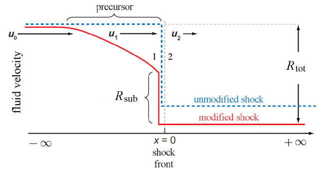
Figure 2: Schematic view of a modified shock. Adapted from Reynolds (2008).

To show this quantitatively, we will present a semi-analytical model of non-linear DSA given by Blasi (2002a,b) (see also Blasi 2004, Blasi et al. 2005, Blasi et al. 2007, Amato & Blasi 2005, Ferrand 2010 and Pavlović 2018).We will assume that we measure everything in the shock frame and that the problem is stationary and one-dimensional. The diffusion-advection equation is then

$$\frac{\partial}{\partial x}\left[D(x,p)\frac{\partial}{\partial x}f(x,p)\right]-u\frac{\partial f(x,p)}{\partial x}+\frac{1}{3}\frac{du}{dx}~{}p~{}\frac{\partial f(x,p)}{\partial p}+Q(x,p)=0,$$ (52)

where $Q(x,p)$ is the so-called injection term, assumed to be in the form $Q(x,p)=Q_{0}(p)\delta(x)$, where $\delta(x)$ is Dirac’s delta function. We saw earlier that momenta in diffusion-advection equation are actually measured in the fluid frame, but if the particles are energetic enough, our choice of the shock frame will not matter much. Particles of a certain momentum $p$ will then diffuse upstream ($x<0$) to some distance

$$x_{p}=\frac{D(p)}{u_{p}},$$ (53)

where $u_{p}$ is some average fluid velocity that will be more precisely defined later. We implicitly assume that the diffusion coefficient is an increasing function of momentum (e.g. linear, $D(p)\propto p$, in the case of Bohm diffusion). The pressure of CR particles will slow down the fluid in the precursor, so that its velocity will change from $u_{0}$ far upstream, to $u_{1}$ immediately ahead of the subshock after which it will drop sharply further to $u_{2}$ downstream.

The first step that we must take is to integrate Eq. (52) across the subshock (from $x=0^{-}$ to $x=0^{+}$, in Fig. 2 these points are marked with 1 and 2, respectively):

$$\left[D\frac{\partial f}{\partial x}\right]_{2}-\left[D\frac{\partial f}{\partial x}\right]_{1}+\frac{1}{3}p\frac{df_{0}}{dp}(u_{2}-u_{1})+Q_{0}(p)=0,$$ (54)

where we have assumed continuity of the distribution function $f_{2}-f_{1}=0$, i.e. $f_{0}=f_{1}=f_{2}$. By assuming a constant distribution function in downstream region (Blasi 2002a, Reynolds 2008), that is $\left[D\frac{\partial f}{\partial x}\right]_{2}=0$, the last equation becomes:

$$\left[D\frac{\partial f}{\partial x}\right]_{1}=\frac{1}{3}p\frac{df_{0}}{dp}(u_{2}-u_{1})+Q_{0}(p).$$ (55)

The next step is to perform integration of Eq. (52) again, but now from $x=-\infty$ to $x=0^{-}$. By using Eq. (55) and applying partial integration

$$\int_{-\infty}^{0^{-}}u\frac{\partial f}{\partial x}dx=\left[uf\right]_{-\infty}^{0^{-}}-\int_{-\infty}^{0^{-}}f\frac{du}{dx}dx,$$

we get:

$$\frac{1}{3}p\frac{df_{0}}{dp}(u_{2}-u_{1})-u_{1}f_{0}+Q_{0}(p)+\int_{-\infty}^{0^{-}}f\frac{du}{dx}dx+\frac{1}{3}\int_{-\infty}^{0^{-}}\frac{du}{dx}p\frac{\partial f}{\partial p}dx=0.$$ (56)

We shall now define

$$u_{p}=u_{1}-\frac{1}{f_{0}}\int_{-\infty}^{0^{-}}\frac{du}{dx}f(x,p)dx,$$ (57)

that represents an average fluid velocity experienced by particles with momentum $p$ while diffusing upstream. As already mentioned, assuming that $D(p)$ is increasing function of momentum, particles of momentum $p$ will reach only to some $x_{p}$ and thus sample only a part of the precursor’s velocity profile. Hence $u_{p}$ can be interpreted physically as some typical fluid velocity at position $x_{p}$. The last term on the left-hand side of Eq. (56) can be transformed to

$$\frac{1}{3}\int_{-\infty}^{0^{-}}\frac{du}{dx}p\frac{\partial f}{\partial p}dx=\frac{1}{3}p\frac{d}{dp}\int_{-\infty}^{0^{-}}f\frac{du}{dx}dx,$$

so that Eq. (56) becomes:

$$\frac{1}{3}p\frac{df_{0}}{dp}(u_{2}-u_{p})-f_{0}\left(u_{p}+\frac{1}{3}p\frac{du_{p}}{dp}\right)+Q_{0}(p)=0,$$ (58)

where we used

$$p\frac{d}{dp}\int_{-\infty}^{0^{-}}\frac{du}{dx}fdx=p\left(\frac{df_{0}}{dp}(u_{1}-u_{p})-f_{0}\frac{du_{p}}{dp}\right),$$

which follows from the definition of $u_{p}$. Eq. (58) represents an ordinary linear differential equation for $f_{0}(p)$ when $u_{p}$ is known and can be integrated to give:

$$f_{0}(p) = \int_{p_{0}}^{p}\frac{d{\bar{p}}}{{\bar{p}}}\frac{3Q_{0}({\bar{p}})}{u_{\bar{p}}-u_{2}}\exp\left\{-\int_{\bar{p}}^{p}\frac{dp^{\prime}}{p^{\prime}}\frac{3}{u_{p^{\prime}}-u_{2}}\left[u_{p^{\prime}}+\frac{1}{3}p^{\prime}\frac{du_{p^{\prime}}}{dp^{\prime}}\right]\right\}$$ (59)

$$= \frac{3R_{\rm{sub}}}{R_{\rm{sub}}-1}\frac{\eta n_{\rm{1}}}{4\pi p_{\rm{inj}}^{3}}\cdot\exp\left\{-\int_{p_{\rm{inj}}}^{p}\frac{dp^{\prime}}{p^{\prime}}\frac{3}{u_{p^{\prime}}-u_{2}}\left[u_{p^{\prime}}+\frac{1}{3}p^{\prime}\frac{du_{p^{\prime}}}{dp^{\prime}}\right]\right\}\!\!.$$

In the above equation we have assumed monochromatic injection of particles with momentum $p_{\rm{inj}}$: $Q_{0}(p)=\frac{\eta n_{\rm{1}}u_{1}}{4\pi p_{\rm{inj}}^{2}}\delta(p-p_{\rm{inj}})$, where $n_{\rm{1}}$ is gas number density immediately upstream ($x=0^{-}$) and $\eta$ is the injection efficiency giving the percentage of particles encountering the shock that are injected into the acceleration process. We have $n_{\rm{1}}=n_{0}R_{\rm{tot}}/R_{\rm{sub}}=n_{0}R_{\rm{prec}}$, where $n_{0}$ ia ambient density, $R_{\rm{sub}}=u_{1}/u_{2}$ is the compression at the subshock, $R_{\rm{tot}}=u_{0}/u_{2}$ is the total shock compression and $R_{\rm{prec}}=u_{0}/u_{1}=R_{\rm{tot}}/R_{\rm{sub}}$ is the compression in the precursor. While in the case of unmodified strong adiabatic shock Rankine-Hugoniot jump conditions give $R=4$, here usually $R_{\rm{sub}}<4$ and $R_{\rm{tot}}>4$.

Blasi’s model of injection (Blasi et al. 2005) assumes that

$$p_{\rm inj}=\xi p_{\rm th,2},$$ (60)

where thermal momentum is $p_{\rm th,2}=\sqrt{2m_{\rm p}kT_{2}}$, $T_{2}$ is downstream temperature and $\xi$ is an injection parameter that can be related to injection efficiency, from now on designated as $\eta$), by requiring continuity of thermal (Maxwell) and non-thermal distribution downstream at $p_{\rm inj}$, that is $f_{\rm th}(p_{\rm inj})=f_{0}(p_{\rm inj})$. From this condition one can find:

$$\eta=\frac{4}{3\sqrt{\pi}}(R_{\rm sub}-1)\xi^{3}e^{-\xi^{2}},$$ (61)

where factor $R_{\rm sub}-1$ serves as a kind of regulator – injection is switched off when $R_{\rm sub}\rightarrow 1$ i.e. subshock gets smoothed.

If we define dimensionless average fluid velocity $U(p)=U_{p}=u_{p}/u_{0}$, Eq. (59) finally becomes:

$$f_{0}(p)=\left(\frac{3R_{\rm{sub}}}{R_{\rm{tot}}U(p)-1}\right)\frac{\eta n_{\rm{1}}}{4\pi p_{\rm{inj}}^{3}}\cdot\exp\left\{-\int_{p_{\rm{inj}}}^{p}\frac{dp^{\prime}}{p^{\prime}}\frac{3R_{\rm{tot}}U(p^{\prime})}{R_{\rm{tot}}U(p^{\prime})-1}\right\}.$$ (62)

If $U_{p}\equiv 1$, then $R_{\rm{tot}}=R_{\rm{sub}}=R$, and we recover the test-particle solution $f_{0}\propto p^{-3R/(R-1)}$. The non-linearity of the problem lies in the fact that $U_{p}\neq$ const. and generally $f_{0}(p)$ will depend on velocity profile $U_{p}$ through Eq. (62), but $U_{p}$ itself will depend on $f(p)$, in a non-linear fashion.

To find $U_{p}$ we will use momentum conservation equation that relates quantities far upstream ($x\to-\infty$) with the quantities at $x_{p}$ where fluid velocity is $u_{p}$:

$$\rho_{0}u_{0}^{2}+P_{\mathrm{th},0}+P_{\mathrm{CR},0}+P_{\mathrm{w},0}=\rho_{p}u_{p}^{2}+P_{\mathrm{th},p}+P_{\mathrm{CR},p}+P_{\mathrm{w},p}.$$ (63)

In the above equation $\rho$ is the density, $P_{\rm{th}}$ the thermal pressure, $P_{\rm{CR}}$ the non-thermal CR pressure and $P_{\rm{w}}$ the pressure of MHD waves.

In the adiabatic approximation

$$\frac{P_{\mathrm{th},p}}{P_{\mathrm{th},0}}=\left(\frac{\rho_{p}}{\rho_{0}}\right)^{\gamma}=\left(\frac{u_{0}}{u_{p}}\right)^{\gamma}=U_{p}^{-\gamma},$$ (64)

where we used mass conservation equation $\rho_{0}u_{0}=\rho_{p}u_{p}$. In the case of Alfvén heating of plasma Berezhko & Ellison (1999) suggested a modification to Eq. (64):

$$\frac{P_{\mathrm{th},p}}{P_{\mathrm{th},0}}=U_{p}^{-\gamma}\left[1+\zeta(\gamma-1)\frac{M_{\mathrm{S},0}^{2}}{M_{\mathrm{A},0}}(1-U_{p}^{\gamma})\right],$$ (65)

where $M_{\mathrm{S},0}=\frac{u_{0}}{c_{\mathrm{S},0}}$ is the Mach’s number, $c_{\mathrm{S},0}=\sqrt{\gamma P_{\mathrm{th},0}/\rho_{0}}$ ambient sound speed, $M_{\mathrm{A},0}=u_{0}/\upsilon_{\mathrm{A},0}$ the Alfvén-Mach number, with $\upsilon_{\mathrm{A},0}$ being the Alfvén speed. The Alfvén heating parameter $0\leq\zeta\leq 1$ was introduced later by Caprioli et al. (2009). For $\zeta=0$ we recover Eq. (64), i.e. no Alfvén heating, while for $\zeta=1$ there is efficient heating, but then, as we shall soon see, there is no magnetic field amplification.

Let us just note here that one of the most interesting discoveries, which came out of the magnetic field determination using X-ray observations of several young SNRs, was that the magnetic fields in SNRs were typically $\sim 100\ \mathrm{\mu G}$, much larger than might be expected, if they were only caused by the compression of the IS magnetic field of $\sim 5\ \mathrm{\mu G}$ (Vink 2012, Uchiyama et al. 2007). Such high magnetic fields indicate that some kind of a magnetic field amplification mechanism is operating in these young SNRs. Bell (2004) suggested that magnetic field amplification might be due to a particular plasma instability induced by the streaming of CR protons away from shocks. Another possibility is to amplify the field as a result of the turbulence induced by the cosmic-ray gradient upstream of the shock acting on an inhomogeneous ambient medium (so-called Drury instability; Drury & Downes 2012). The effectiveness of such processes in magnetic field amplification to the level needed to accelerate CRs up to the PeV domain is still debated in the present literature.

For the CR pressure in Eq. (63) we will assume $P_{\rm{CR},0}=0$ (no CR particles far upstream) and since only the particles with momentum $\geq p$ can reach $x=x_{p}$, we have:

$$P_{\mathrm{CR},p}=\frac{4\pi}{3}\int_{p}^{p_{\mathrm{max}}}p^{3}v(p)f_{0}(p)dp=\frac{4\pi}{3}\int_{p}^{p_{\mathrm{max}}}\frac{p^{4}c^{2}}{\sqrt{m_{\mathrm{p}}^{2}c^{4}+p^{2}c^{2}}}f_{0}(p)dp,$$ (66)

where $v(p)$ is particle speed and $p_{\mathrm{max}}$ is the maximum momentum reached by CR particles which depends on the relevant time-scale of acceleration, escape and losses (Blasi et al. 2007).

Similarly to CR pressure, we will assume that MHD waves pressure $P_{\rm{w},0}=0$ far upstream. In the precursor, closer to the subshock, CR themselves will generate magnetic turbulence (necessary for their scattering and thus acceleration). This turbulent field will generally have an amplitude larger than the regular field $B_{0}$ and it can be assumed that this turbulent magnetic field pressure will be some fraction $\alpha<1$ of the CR pressure

$$P_{\mathrm{w},p}=\alpha P_{\mathrm{CR},p}.$$ (67)

Based on the quasi-linear theory $\alpha\sim\upsilon_{\mathrm{A},0}/u_{0}$ for the resonant streaming instability (Caprioli et al. 2009), while for the non-resonant instability $\alpha\sim u_{0}/c$ (Bell 2004). Caprioli et al. (2009) suggested that

$$\frac{P_{\mathrm{w},p}}{\rho_{0}u_{0}^{2}}=\frac{1-\zeta}{4M_{\mathrm{A},0}}U_{p}^{-3/2}(1-U_{p}^{2}),$$ (68)

where $U_{p}^{-3/2}$ is adiabatic compression of the field, and factor $1-\zeta$ account for the Alfvén heating in Eq. (65) – the wave dumping (and thus the gas heating) must remain reasonably small for the magnetic field to be substantially amplified ($\zeta<1$).

Setting $P_{\rm{CR},0}$, $P_{\rm{w},0}$ = 0, in Eq. (63), dividing by $\rho_{0}u_{0}^{2}$ and inserting Eqs. (65), (66) and (68), we obtain:

$$U_{p}+\frac{U_{p}^{-\gamma}}{\gamma M_{\mathrm{S},0}^{2}}\left[1+\zeta(\gamma-1)\frac{M_{\mathrm{S},0}^{2}}{M_{\mathrm{A},0}}(1-U_{p}^{\gamma})\right]+\frac{4\pi}{3\rho_{0}u_{0}^{2}}\int_{p}^{p_{\rm max}}dpp^{3}v(p)f_{0}(p)$$

$$+\frac{1-\zeta}{4M_{\mathrm{A},0}}U_{p}^{-3/2}(1-U_{p}^{2})=1+\frac{1}{\gamma M_{\mathrm{S},0}^{2}}.\ \ \$$ (69)

Deriving the last equation with respect to $p$ we get, finally:

$$\frac{dU_{p}}{dp}\left\{1-\frac{U_{p}^{-(\gamma+1)}}{M_{\mathrm{S},0}^{2}}\left[1+\zeta(\gamma-1)\frac{M_{\mathrm{S},0}^{2}}{M_{\mathrm{A},0}}\right]-\frac{1-\zeta}{8M_{\mathrm{A},0}}\frac{U_{p}^{2}+3}{U_{p}^{5/2}}\right\}$$

$$=\frac{4\pi}{3\rho_{0}u_{0}^{2}}p^{3}\upsilon(p)f_{0}(p).$$ (70)

Now that we have Eqs. (58) and (70), we need to know all the parameters appearing in them and the boundary conditions. For fixed Mach and Alfvén-Mach numbers (that is velocity $u_{0}$ and parameters of the surroundings $\rho_{0},P_{0},B_{0},\gamma$), $\eta$, $\zeta$, $p_{\rm max}$, we must find another relation between $R_{\rm sub},R_{\rm tot},R_{\rm prec}$ (knowing that by the definition $R_{\rm tot}=R_{\rm sub}\cdot R_{\rm prec}$), and calculate $p_{\mathrm{inj}}$. We shall accomplish this by considering jump conditions at the subshock. Let us start with the momentum conservation equation:

$$\rho_{1}u_{1}^{2}+P_{\mathrm{th},1}+P_{\mathrm{CR},1}+P_{\mathrm{w},1}=\rho_{2}u_{2}^{2}+P_{\mathrm{th},2}+P_{\mathrm{CR},2}+P_{\mathrm{w},2}.$$ (71)

CR pressure must be continuous across the subshock $P_{\mathrm{CR},1}=P_{\mathrm{CR},2}$, while for the thermal pressure Vainio & Schlickeiser (1999) derived a modified Rankine-Hugoniot jump conditions in the presence of plasma’s MHD waves

$$\frac{P_{\rm th,2}}{P_{\rm th,1}}=\frac{(\gamma+1)R_{\rm sub}-(\gamma-1)\left[1-(R_{\rm sub}-1)\Delta\right]}{(\gamma+1)-(\gamma-1)R_{\rm sub}},$$ (72)

where

$$\Delta=\frac{R_{\rm sub}+1}{R_{\rm sub}-1}\frac{[P_{\rm w}]^{2}_{1}}{P_{\rm th,1}}-\frac{2R_{\rm sub}}{R_{\rm sub}-1}\frac{[F_{\rm w}]^{2}_{1}}{P_{\rm th,1}u_{1}},$$ (73)

and $[P_{\rm w}]^{2}_{1}$, $[F_{\rm w}]^{2}_{1}$ are jumps in magnetic field pressure and magnetic energy flux, respectively (we will use notation $[Y]^{2}_{1}=Y_{2}-Y_{1}$). In the case $\Delta=0$, we obtain the standard Rankine-Hugoniot jump condition.

Caprioli et al. (2008, 2009) found $[P_{\rm w}]^{2}_{1}$ and $[F_{\rm w}]^{2}_{1}$ for the MHD waves, by considering their transmission and reflection: $[P_{\rm w}]^{2}_{1}=(R_{\rm sub}^{2}-1)P_{\rm w,1}$, $[F_{\rm w}]^{2}_{1}=2(R_{\rm sub}-1)P_{\rm w,1}u_{1}$, which when inserted in Eq. (72) give:

$$\frac{P_{\rm th,2}}{P_{\rm th,1}}=\frac{(\gamma+1)R_{\rm sub}-(\gamma-1)\left[1-(R_{\rm sub}-1)^{3}\frac{P_{\rm w,1}}{P_{\rm th,1}}\right]}{(\gamma+1)-(\gamma-1)R_{\rm sub}}.$$ (74)

Eq. (71), assuming $P_{\rm CR,1}=P_{\rm CR,2}$, can be transformed to:

$$\frac{\rho_{1}u_{1}^{2}}{P_{\rm w,1}}\frac{R_{\rm sub}-1}{R_{\rm sub}}+\frac{P_{\rm th,1}}{P_{\rm w,1}}\left(\frac{P_{\rm th,2}}{P_{\rm th,1}}-1\right)+R_{\rm sub}^{2}-1=0.$$ (75)

Let us introduce Mach’s number ahead of the subshock $M_{\rm S,1}=u_{1}/c_{\rm S,1}$, where $c_{\rm S,1}=\sqrt{\gamma P_{\rm th,1}/\rho_{1}}$, that can be related to $M_{\rm S,0}$ by using Eq. (65):

$$\frac{M_{\rm S,1}^{2}}{M_{\rm S,0}^{2}}=\frac{\rho_{1}u_{1}^{2}}{\rho_{0}u_{0}^{2}}\frac{P_{\rm th,0}}{P_{\rm th,1}}=R_{\rm prec}^{-\gamma-1}\left[1+\zeta(\gamma-1)\frac{M_{\mathrm{S},0}^{2}}{M_{\mathrm{A},0}}(1-R_{\rm prec}^{-\gamma})\right]^{-1}.$$ (76)

Finally, from Eqs. (74) and (75), after some algebra, we find:

$$M_{\rm S,1}^{2}=\frac{2R_{\rm sub}}{(\gamma+1)-(\gamma-1)R_{\rm sub}-2R_{\rm sub}P_{\rm w,1}^{*}\left[\gamma-(\gamma-2)R_{\rm sub}\right]},$$ (77)

where we introduced:

$$P_{\rm w,1}^{*}=\frac{P_{\rm w,1}}{\rho_{1}u_{1}^{2}}=R_{\rm prec}\frac{P_{\rm w,1}}{\rho_{0}u_{0}^{2}}=\frac{1-\zeta}{4M_{\rm A,0}}R_{\rm prec}^{5/2}(1-R_{\rm prec}^{-2}).$$ (78)

When we can neglect MHD waves, $P_{\rm w,1}\simeq 0$, Eq. (77) gives standard Rankine-Hugoniot relation:

$$M_{\rm S,1}^{2}=\frac{2R_{\rm sub}}{(\gamma+1)-(\gamma-1)R_{\rm sub}}\Longleftrightarrow R_{\rm sub}=\frac{\gamma+1}{\frac{2}{M_{\rm S,1}^{2}}+\gamma-1}.$$ (79)

If $P_{\rm w,1}>0$, for fixed $R_{\rm prec}$, Eq. (77) is quadratic in $R_{\rm sub}$:

$$2(\gamma-2)M_{\rm S,1}^{2}P_{\rm w,1}^{*}R_{\rm sub}^{2}-\left[2+(\gamma-1+2\gamma P_{\rm w,1}^{*})M_{\rm S,1}^{2}\right]R_{\rm sub}+M_{\rm S,1}^{2}(\gamma+1)=0.$$ (80)

Positive root of this equation will give us $R_{\rm sub}$ as a function of $M_{\rm S,1}$ and $P_{\rm w,1}^{*}$, and consequently the total compression $R_{\rm tot}$.

Finally, we need downstream temperature, in order to calculate $p_{\mathrm{inj}}$. By using ideal fluid equation of state $P\propto\rho T$ and Eq. (65), we have

$$\frac{T_{1}}{T_{0}}=\frac{\rho_{0}}{\rho_{1}}\frac{P_{\rm th,1}}{P_{\rm th,0}}=R_{\rm prec}^{\gamma-1}\left[1+\zeta(\gamma-1)\frac{M_{\rm S,0}^{2}}{M_{\rm A,0}}(1-R_{\rm prec}^{-\gamma})\right],$$ (81)

and from Eq. (74)

$$\frac{T_{2}}{T_{1}}=\frac{\rho_{1}}{\rho_{2}}\frac{P_{\rm th,2}}{P_{\rm th,1}}=\frac{(\gamma+1)R_{\rm sub}-(\gamma-1)\left[1-(R_{\rm sub}-1)^{3}\frac{P_{\rm w,1}}{P_{\rm th,1}}\right]}{\left[(\gamma+1)-(\gamma-1)R_{\rm sub}\right]R_{\rm sub}}.$$ (82)

We are now ready for ’shooting for the solution’ with an assumed $R_{\rm prec}$ and the initial conditions

$$U_{p}(p=p_{\rm inj})=U_{p}(x=0^{-})=\frac{u_{1}}{u_{0}}=\frac{1}{R_{\mathrm{prec}}},$$ (83)

$$\lim_{p\to p_{\rm{inj}}}f_{0}(p)=\frac{3R_{\rm{sub}}}{R_{\rm{sub}}-1}\frac{\eta n_{\rm{1}}}{4\pi p_{\rm{inj}}^{3}}.$$ (84)

An arbitrarily chosen $R_{\rm prec}$ will, however, not necessarily satisfy the boundary condition

$$U_{p}(p=p_{\rm{max}})=U_{p}(x=-\infty)=\frac{u_{0}}{u_{0}}=1,$$ (85)

used to end the integration at $p_{\mathrm{max}}$, so the solution needs to be found iteratively. To make things simpler, we will introduce dimensionless variables

$$\frac{p}{m_{\mathrm{p}}c}\rightarrow p,$$

$$\frac{4\pi}{3}\frac{m_{\mathrm{p}}^{4}c^{5}}{\rho_{0}u_{0}^{2}}f_{0}\rightarrow f_{0},$$

and solve simultaneously Eqs. (58) and (70) in the form

$$\frac{1}{3}\Big{(}\frac{1}{R_{\mathrm{tot}}}-U_{p}\Big{)}p\frac{df_{\mathrm{0}}}{dp}-\Big{(}U_{p}+\frac{1}{3}p\frac{dU_{p}}{dp}\Big{)}f_{\mathrm{0}}=0,$$ (86)

$$\frac{dU_{p}}{dp}\Bigg{\{}1-\frac{U_{p}^{-(\gamma+1)}}{M_{\mathrm{S},0}^{2}}\Big{[}1+\zeta(\gamma-1)\frac{M_{\mathrm{S},0}^{2}}{M_{\mathrm{A},0}}\Big{]}-\frac{1-\zeta}{8M_{\mathrm{A},0}}\frac{U_{p}^{2}+3}{U_{p}^{5/2}}\Bigg{\}}=\frac{p^{4}f_{\mathrm{0}}}{\sqrt{1+p^{2}}}.$$ (87)

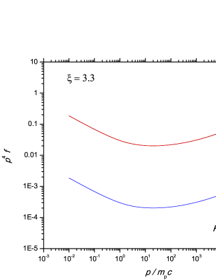
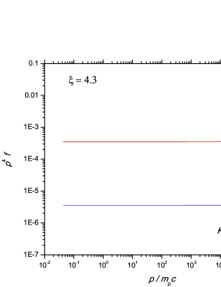
Figure 3: Proton and electron spectra for injection parameter $\xi=3.3$ (left) and $\xi=4.3$ (right).

In Fig. 3 we give the results for two cases: strongly-modified shock ($\xi=3.3$) and a test-particle case ($\xi=4.3$), as in Caprioli et al. (2010). Other parameters in two cases are the same: shock velocity $u_{0}$ = 5000 km/s, ambient density $n_{\mathrm{H}}\sim 0.1\mathrm{cm}^{-3}$, temperature $T_{0}=10^{4}$ K, magnetic field $B_{0}$ = 5.3775 $\mu$G, equal Mach and Alfvén-Mach numbers of 135 and Alfvén heating parameter $\zeta=0.5$. For the case $\xi=3.3$, subshock and the total compressions are $R_{\mathrm{sub}}=3.081$, $R_{\mathrm{tot}}=10.236$, $p_{\mathrm{inj}}=0.01$ and $p_{\mathrm{max}}=3.316\cdot 10^{5}$, while for $\xi$ = 4.3, $R_{\mathrm{sub}}=3.999$, $R_{\mathrm{tot}}=4.018$, $p_{\mathrm{inj}}=0.0437$, $p_{\mathrm{max}}$ is the same. For ’practical’ purposes, e.g. modeling the radio synchrotron emission of astrophysical sources such as supernova remnants (e.g. Berezhko & Völk 2004, Pavlović 2017, Pavlović et. al 2018), besides proton spectrum it is also crucial to know electron spectrum. It is usually assumed that the proton and electron spectra are parallel and that $p_{\mathrm{inj}}$ for protons and electrons are the same (although how this is accomplished for electrons is still uncertain) in order for both CR species to cross and recross the subshock (with an assumed thickness $\approx r_{\rm g}\propto p_{\mathrm{th}}$ of protons) unaffected. The only unknown parameter left is then the electron-to-proton number ratio at high energies $K_{\mathrm{ep}}$, for which in Figs. 3 and 4 we assumed $K_{\mathrm{ep}}=1:100$, in accordance with the observed ratio for Galactic cosmic-rays. The extreme cases presented in Fig. 3 depict a general behavior – shocks with low $\xi\lesssim 3.5$ have high injection efficiency $\eta$ and are highly modified, producing a typical concave-up spectrum; shocks with high $\xi\gtrsim 4$ have low injection efficiency and will produce basically a test-particle spectrum $f_{0}\propto p^{-\mathnormal{\Gamma}-2}$ with $\mathnormal{\Gamma}\approx 2$. It is important to note at the end that these models do not account for losses and particle escape, since it is assumed that $P_{\rm{CR},0}=0$ far upstream (for alternative see e.g. Caprioli et al. 2010).

3 Observational signatures of particle acceleration in ISM: a quick overview

Instead of the summary, we present here a quick overview of the most important observational signatures of particle acceleration in ISM.

As already seen in the previous sections, DSA can be held responsible for the production of the non-thermal ensemble of cosmic-ray particles which in the simplest test-particle case has a power-law energy distribution. Actually, the particle energy spectral index, derived from the theory seems to be in very good accordance with the present observations of primary CRs of non-solar origin in the vicinity of planet Earth ($\mathnormal{\Gamma}\approx 2.7$ up to $\sim 10^{15}\ \mathrm{eV}$).

Furthermore, the presence of ultra-relativistic charged particles moving in the external global magnetic field will generally cause significant production of synchrotron radiation. The history of radio astronomy teaches us that one of the first detected objects that glow in the radio sky are indeed SNRs, in particular Cas A remnant (Reber 1944). In fact, the non-thermal radio-continuum spectra of SNRs, shaped by the synchrotron emission, unambiguously pointed to the presence of high-energy charged particles linked to the IS shock waves. Strictly speaking, however, this only provided the evidence for electron acceleration, whereas the observed CR spectrum in the Earth’s neighborhood consists mainly of protons and other heavy ions. Of course, for massive charges synchrotron radiation is indeed emitted, but at a much lower efficiency. As we noted earlier, protons and heavier particles can be accelerated very efficiently to $\sim 10^{15}\ \mathrm{eV}$. Electrons can also be accelerated to the ultra-relativistic energies ($\sim 10^{12}\ \mathrm{eV}$) by DSA mechanism and this lower maximal energy of electrons comes from the very rapid energy losses induced by the inverse Compton, non-thermal bremsstrahlung and synchrotron radiation.

The energy spectrum of relativistic electrons which is in the form of a power-law in test-particle DSA is transformed in the power-law radio continuum spectrum. The particle energy index from the energy spectrum of CRs can be transformed in the so-called spectral index of the radio spectrum $\alpha$, by the simple linear relation $\mathnormal{\Gamma}=2\alpha+1$. A radio continuum may then be characterized by the power-law form $S_{\nu}\propto\nu^{-\alpha}$, where $S_{\nu}$ is the radio flux density at frequency $\nu$. It is easy to conclude that the value for spectral index derived directly from test-particle DSA theory is 0.5. As we know from the observational data, the large majority of radio spectra of Galactic SNRs have $\alpha=0.5$ (more generally between 0.2 and 0.8; see Green 2017 as well as Urošević 2014, for more details). This really seems to be an excellent confirmation of the theoretical predictions. Furthermore, for a standard value of the mean Galactic magnetic field strength ($\sim 5\ \mu\mathrm{G}$), GeV electrons are responsible for the synchrotron emission at higher radio-frequencies, and TeV electrons for X-rays.

X-ray synchrotron emission that is linked to the SNRs is usually associated with the existence of a pulsar wind nebula (or plerion). Still, over the last several decades the evidence for electron acceleration in SNRs has been significantly enhanced by the detection of X-ray synchrotron radiation from the shells of several young remnants (Koyama et al. 1995). This X-ray synchrotron emission implies that CR electrons are indeed accelerated up to energies of around 10 to 100 TeV. Furthermore, such young SNRs generally have an X-ray synchrotron spectra with rather steep indices $\mathnormal{\Gamma}=2-3.5$ which points to a steep underlying electron energy distribution. Such a detected steepness, on the other hand, indicates that the synchrotron X-ray emission is in fact caused by the electrons close to the maximum energy of the CRs electron energy distribution.

Furthermore, $\gamma$-ray observations are a promising way to study CR acceleration in the SNRs, especially in the TeV and even PeV range (e.g. Gaggero et al. 2018). We note here that the $\gamma$-rays may not necessarily come from the pulsars and pulsar wind nebulae, but from the SNR shells, too. The Cherenkov $\gamma$-ray telescopes (like H.E.S.S., MAGIC and VERITAS) have detected around 16 TeV sources that are associated with SNRs, while few tens of firm identifications at GeV energies are present in the first Fermi catalogue of SNRs (Acero et al. 2016). The great importance of $\gamma$-ray astronomy is reflected in the fact that it can give us a direct view of the CR nuclei, accelerated via DSA. These cosmic-ray protons and heavy ions produce $\gamma$-ray emission if they collide with the ambient IS atomic nuclei. As a result, among the other products of such a collision process, neutral pions are created, which then decay in two $\gamma$-ray photons (the so-called hadronic scenario). This allow us to trace high-energy CRs above GeV energy (see Inoue 2019, and references therein). However, two other important $\gamma$-ray radiation processes originate from CR electrons (the so-called leptonic scenario). Interactions with background photons result in the inverse Compton up-scattering, whereas interactions with ions in the SNR result in bremsstrahlung radiation. Usually, inverse Compton scattering is a more dominant leptonic process in young SNRs. However, it is generally very difficult to distinguish between hadronic and leptonic origin of $\gamma$-rays (Sano et al. 2019). The advanced TeV and other $\gamma$-ray telescopes like the Cherenkov Telescope Array could in principle help us to infer more on the role of SNRs in the efficient CR production.

In the case of very young SNRs, i.e. strong collisonless shocks, we expect that the effects of the non-linear DSA can cause a slightly concave up synchrotron spectrum (Reynolds & Ellison 1992, Jones et al. 2003, de Looze et al. 2017). In fact, from Section 2.4, we have learned that a non-linear DSA theory predicts that the particle energy spectrum steepens at low energies and also flattens at higher energies. This immediately leads to the curved synchrotron (radio to microwave continuum) spectrum, that can be crudely modeled by a pure power-law with a varying spectral index, such as in the case of famous SNR Cas A (Onić & Urošević 2015). Of course, further observations of the integrated radio up to microwave continuum of SNRs is of great importance as any possible deviations from the known theory can give us new clues about physics of the observed emission. We need reliable flux density estimates at as many as possible different continuum frequencies. However, this is connected with serious observational problems, such as transparency issues regarding the Earth’s atmosphere. The new confirmations of the theoretically predicted radio spectral features at high radio frequencies could be expected from future observations by for instance, ALMA (Atacama Large Millimeter/submillimeter Array) telescope. As a final note, another consequence of the spectral curvature is that the actual X-ray synchrotron brightness cannot be just simply estimated from an extrapolation of the radio synchrotron spectrum – it should be brighter than the one expected (Vink et al. 2006, Allen et al. 2008).

Finally, a word of caution regarding the non-linear DSA theory presented earlier in this paper. Several authors claim that the concavity of the spectrum contradicts present $\gamma$-ray observations (see e.g. Caprioli 2011). One way of removing the concavity was found in Ferrand et al. (2014). It was shown that at perpendicular shocks, the concavity can be removed by replacing the Bohm diffusion coefficient by a more realistic form.

Another important question is related to the observational fact that several young pre-Sedov SNRs exhibit rather steep (but not curved) radio spectral indices ($\alpha>0.5$). Neglecting the non-linear hydrodynamic effects due to the CR pressure in the precursor, Bell et al. (2011) demonstrated that the oblique-shock effects can produce a steep spectrum if the high velocity shock of a young SNR has a tendency towards a quasi-perpendicular configuration. They noted that either a magnetic field amplification in the precursor due to CR streaming or expansion into a circumstellar wind supporting a Parker spiral may produce a quasi-perpendicular shock geometry. Bell et al. (2011) also concluded that the Galactic CR spectrum is most probably formed by a complex mixture of non-linear, oblique-shock and momentum-dependent CR escape effects. In the case of large shock inclinations, acceleration efficiency decreases and one would expect steeper spectrum. However, acceleration efficiency for shock inclinations greater than $60^{\circ}$ is found to be decreasing, reaching practically zero percent (see Figure 3 in Caprioli & Spitkovsky 2014) and quenching particle acceleration (except in the case of diffusive shock re-acceleration mechanism). Spectral steepening in young SNRs has also been discussed by Bell et al. (2019). They proposed a new process in which the loss of CR energy to turbulence and magnetic field during the CR acceleration at the non-relativistic quasi-parallel shocks is responsible for the spectral steepening. One should bear in mind that such a process is indeed a non-linear effect in the sense that it depends on the shock velocity and on non-linear turbulent amplification of magnetic field, but it does not depend on the ratio of the CR pressure to the kinetic pressure at the shock. On the other hand, using particular numerical simulation that incorporates three-dimensional hydrodynamic modeling and non-linear kinetic theory of CR acceleration in parallel shocks, taking into account the non-linear back reaction of accelerated particles on the fluid structure, Pavlović (2017) found that the steep (but not significantly curved) radio spectral index of the youngest known SNR G1.9+0.3 can be solely explained by means of the efficient NLDSA. The most probable scenario is the one that incorporates more than one of the proposed processes that act at the same time.

In addition, a significant contribution of the second order Fermi (or stochastic) acceleration mechanism is usually proposed to shape the radio-continuum of several evolutionary old Galactic SNRs with spectral indices $\alpha$ less than 0.5 (Schlickeiser & Fürst 1989, Ostrowski 1999). However, contribution of the secondary electrons left over from the decay of charged pions (if an SNR is interacting with a molecular cloud), or just a simple thermal contamination, or even the intrinsic thermal bremsstrahlung radiation from the SNRs, etc., can also cause such flat spectral indices as observed in some, usually evolutionary old SNRs in high density environment (Uchiyama et al. 2010, Onić 2013).

- (1) Acero F, Ackermann M, Ajello M, Baldini L, Ballet J, Barbiellini G, Bastieri D, Bellazzini R, Bissaldi E, Blandford RD, et al (2016) The First Fermi LAT Supernova Remnant Catalog. Astrophys J Sup 224:8-58
- (2) Allen GE, Houck JC, Sturner SJ (2008) Evidence of a curved synchrotron spectrum in the supernova remnant SN 1006. Astrophys J 683:773-785
- (3) Amato E, Blasi P (2005) A general solution to non-linear particle acceleration at non-relativistic shock waves. Mon Not R Astron Soc 364:L76-L80
- (4) Arbutina B (2017) Evolution of supernova remnants. Publ Astron Obs Belgrade 97:1-92
- (5) Axford WI, Leer E, Skadron G (1977) The acceleration of cosmic-rays by shock waves. International Cosmic Ray Conference 11:132-137
- (6) Bell AR (1978a) The acceleration of cosmic-rays in shock fronts. I. Mon Not R Astron Soc 182:147-156
- (7) Bell AR (1978b) The acceleration of cosmic-rays in shock fronts. II. Mon Not R Astron Soc 182:443-455
- (8) Bell AR (2004) Turbulent amplification of magnetic field and diffusive shock acceleration of cosmic-rays. Mon Not R Astron Soc 353:550-558
- (9) Bell AR, Matthews JH., Blundell KM (2019) Cosmic ray acceleration by shocks: spectral steepening due to turbulent magnetic field amplification. Mon Not R Astron Soc 488:2466-2472
- (10) Bell AR, Schure KM, Reville B (2011) Cosmic ray acceleration at oblique shocks. Mon Not R Astron Soc 418:1208-1216
- (11) Bell AR, Schure KM, Reville B, Giacinti, G (2013) Cosmic-ray acceleration and escape from supernova remnants. Mon Not R Astron Soc 431:415-429
- (12) Berezhko EG, Ellison HJ (1999) A simple model of nonlinear diffusive shock acceleration. Astrophys J 526:385-399
- (13) Blandford RD, Ostriker JP (1978) Particle acceleration by astrophysical shocks. Astrophys J 221:L29-L32
- (14) Blandford RD, Eichler D (1987) Particle acceleration at astrophysical shocks: a theory of cosmic-ray origin. Phys Rep 154(1):1-75
- (15) Blasi P (2002a) A novel approach to non linear shock acceleration. Nucl Phys B Proc Suppl 110:475-477
- (16) Blasi P (2002b) A semi-analytical approach to non-linear shock acceleration. Astropart Phys 16:429-439
- (17) Blasi P (2004) Nonlinear shock acceleration in the presence of seed particles. Astropart Phys 21:45-57
- (18) Blasi P (2010) Shock acceleration of electrons in the presence of synchrotron losses - I. Test-particle theory. Mon Not R Astron Soc 402:2807-2816
- (19) Blasi P, Gabici S, Vannoni G (2005) On the role of injection in kinetic approaches to non-linear particle acceleration at non-relativistic shock waves. Mon Not R Astron Soc 361:907-918
- (20) Blasi P, Amato E, Caprioli D (2007) The maximum momentum of particles accelerated at cosmic-ray modified shocks. Mon Not R Astron Soc 375:1471-1478
- (21) Caprioli D (2011) Understanding hadronic gamma-ray emission from supernova remnants. Journal of Cosmology and Astroparticle Physics, 5:26
- (22) Caprioli D, Amato E, Blasi P (2010) Non-linear diffusive shock acceleration with free-escape boundary. Astropart Phys 33:307-311
- (23) Caprioli D, Blasi P, Amato E, Vietri M (2008) Dynamical effects of self-generated magnetic fields in cosmic-ray-modified shocks. Astrophys J Lett 679:L139-L142
- (24) Caprioli D, Blasi P, Amato E, Vietri M (2009) Dynamical feedback of self-generated magnetic fields in cosmic-ray modified shocks. Mon Not R Astron Soc 395:895-906
- (25) Caprioli D, Pop A, Spitkovsky A (2015) Simulations and Theory of Ion Injection at Non-relativistic Collisionless Shocks. Astrophys J Lett 798:L28
- (26) Caprioli D, Spitkovsky A (2014) Simulations of ion acceleration at non-relativistic shocks. I. Acceleration efficiency. Astrophys J 783:91-107
- (27) Caprioli D, Zhang H, Spitkovsky A (2018) Diffusive shock re-acceleration. J Plasma Phys 84:715840301
- (28) de Looze I, Barlow MJ, Swinyard BM, Rho J, Gomez, HL, Matsuura M, Wesson R (2017) The dust mass in Cassiopeia A from a spatially resolved Herschel analysis. Mon Not R Astron Soc 465:3309-3342
- (29) Drury LO’C (1983) An introduction to the theory of diffusive shock acceleration of energetic particles in tenuous plasmas. Rep Prog Phys 46:973-1027
- (30) Drury LO’C, Downes TP (2012) Turbulent magnetic field amplification driven by cosmic ray pressure gradients. Mon Not R Astron Soc 427:2308-2313
- (31) Drury LO’C, Völk HJ (1981) Hydromagnetic shock structure in the presence of cosmic-rays. Astron Astrophys 248:344-351
- (32) Drury LO’C, Strong, AW (2015) Cosmic-ray diffusive reacceleration: a critical look. The 34th International Cosmic Ray Conference (arXiv:1508.02675v1)
- (33) Eichler D (1984) On the theory of cosmic-ray-mediated shocks with variable compression ratio. Astrophys J 277:429-434
- (34) Fermi E (1949) On the origin of the cosmic radiation. Phys Rev 75:1169-1174
- (35) Ferrand G (2010) Blasi’s semi-analytical kinetic model of non-linear diffusive shock acceleration. Personal notes
- (36) Ferrand G, Danos R. J, Shalchi A, Safi-Harb S, Edmon P, Mendygral P (2014) Cosmic Ray Acceleration at Perpendicular Shocks in Supernova Remnants. Astrophys J 792:133-145
- (37) Gaggero D, Zandanel F, Cristofari P, Gabici S (2018) Time Evolution of Gamma Rays from Supernova Remnants. Mon Not R Astron Soc 475:5237-5245
- (38) Ginzburg VL, Syrovatskii SI (1967) Cosmic rays in the Galaxy (Introductory Report). In: Radio Astronomy and the Galactic System (ed. H van Woerden), vol. 31 of IAU Symposium, pp. 411
- (39) Green DA (2017) A Catalogue of Galactic Supernova Remnants (2017 June version). Cavendish Laboratory, Cambridge, United Kingdom (available at ”http://www.mrao.cam.ac.uk/surveys/snrs/”)
- (40) Hussein M., Shalchi A (2014) Detailed Numerical Investigation of the Bohm Limit in Cosmic Ray Diffusion Theory. Astrophys J 785:31-37
- (41) Inoue T (2019) Bell-instability-mediated Spectral Modulation of Hadronic Gamma-Rays from a Supernova Remnant Interacting with a Molecular Cloud. Astrophys J 872:46-54
- (42) Jones TJ, Rudnick L, DeLaney T, Bowden J (2003) The identification of infrared synchrotron radiation from Cassiopeia A. Astrophys J 587:227-234
- (43) Koyama K, Petre R, Gotthelf EV, Hwang U, Matsuura M, Ozaki M, Holt SS (1995) Evidence for Shock Acceleration of High-Energy Electrons in the Supernova Remnant SN 1006. Nat 378:255-258
- (44) Krymsky GF (1977) A regular mechanism for the acceleration of charged particles on the front of a shock wave. Akademiia Nauk SSSR Doklady 234:1306-1308
- (45) Lequeux J (2005) The interstellar medium, with the collaboration of E Falgarone and C Ryter. Springer-Verlag, Berlin, Heidelberg
- (46) Longair MS (2011) High energy astrophysics. Volume 2. Stars, the Galaxy and the interstellar medium. Cambridge University Press, Cambridge (UK)
- (47) Malkov MA., Drury LO’C. (2001) Nonlinear theory of diffusive acceleration of particles by shock waves. Rep Prog Phys 64:429-481
- (48) Onić D (2013) On the supernova remnants with flat radio spectra. Astrophys Space Sci 346:3-13
- (49) Onić D, Urošević D (2015) On the Continuum Radio Spectrum of Cas A: Possible Evidence of Non-Linear Particle Acceleration. Astrophys J 805:119-125
- (50) Ostrowski M (1999) Supernova remnants in molecular clouds: on cosmic-ray electron spectra. Astron Astrophys 345:256-258
- (51) Parker E (1965), The passage of energetic charged particles through interplanetary space. Planet Space Sci 13:9-49
- (52) Pavlović MZ (2017) Hydrodynamical and radio evolution of young supernova remnant G1.9+0.3 based on the model of diffusive shock acceleration. Mon Not R Astron Soc 468:1616-1630
- (53) Pavlović MZ (2018) Modeling the radio-evolution of supernova remnants by using hydrodynamic simulations and non-linear diffusive shock acceleration. PhD thesis, University of Belgrade
- (54) Pavlović MZ, Urošević D, Arbutina B, Orlando S, Maxted N, Filipović M (2018) Radio evolution of supernova remnants including nonlinear particle acceleration: insights from hydrodynamic simulations. Astrophys J 858:84
- (55) Reber G (1944) Cosmic Static. Astrophys J 100:279-287
- (56) Reynolds SP, Ellison DC (1992) Electron acceleration in Tycho’s and Kepler’s supernova remnants - spectral evidence of Fermi shock acceleration. Astrophys J 399:L75-L78
- (57) Sano H, Rowell G, Reynoso EM, Jung-Richardt J, Yamane Y, Nagaya T, Yoshiike S, Hayashi K, Torii K, Maxted N, Mitsuishi I, Inoue T, Inutsuka S, Yamamoto H, Tachihara K, Fukui Y (2019) Possible Evidence for Cosmic-Ray Acceleration in the Type Ia Supernova Remnant RCW 86: Spatial Correlation between TeV Gamma rays and Interstellar Atomic Protons. Accepted for publication in Astrophys J (https://arxiv.org/abs/1805.10647)
- (58) Schlickeiser R, Fürst E (1989) The origin of flat radio spectra in shell-type supernova remnants. Astron Astrophys 219:192-194
- (59) Shalchi A (2009) Diffusive shock acceleration in supernova remnants: On the validity of the Bohm limit. Astropart Phys, 31:237-242
- (60) Shalchi A, Skoda T, Tautz R C, Schlickeiser R (2009) Analytical description of nonlinear cosmic ray scattering: isotropic and quasilinear regimes of pitch-angle diffusion. Astron Astrophys 507:589-597
- (61) Skilling J (1971) Cosmic rays in the Galaxy: convection or diffusion. Astrophys J 170:265-273
- (62) Skilling J (1975) Cosmic ray streaming. I - Effect of Alfven waves on particles. Mon Not R Astron Soc 172:557-566
- (63) Uchiyama Y, Aharonian FA, Tanaka T, Takahashi T, Maeda Y (2007) Extremely fast acceleration of cosmic rays in a supernova remnant. Nat 449:576-578
- (64) Uchiyama Y, Blandford RD, Funk S, Tajima H, Tanaka T (2010) Gamma-ray emission from crushed clouds in supernova remnants. Astrophys J 723:L122-L126
- (65) Urošević D (2014) On the radio spectra of supernova remnants. Astrophys Space Sci 354:541-552
- (66) Vainio R, Schlickeiser R (1999) Self-consistent Alfven-wave transmission and test-particle acceleration at parallel shocks. Astron Astrophys 343: 303-311
- (67) Vink J (2012) Supernova remnants: the X-ray perspective. Astron Astrophys Rev 20:49
- (68) Vink J, Bleeker J, van der Heyden K, Bykov A, Bamba A, Yamazak R (2006) The X-ray synchrotron emission of RCW 86 and the implications for its age. Astrophys J 648:L33-L37
- (69) Zeković V (2019) Resonant micro-instabilities at quasi-parallel collisionless shocks: cause or consequence of shock (re)formation. Phys Plasmas 26:032106(1-17)