A BSDE-based approach for the optimal reinsurance problem under partial information

Abstract

We investigate the optimal reinsurance problem under the criterion of maximizing the expected utility of terminal wealth when the insurance company has restricted information on the loss process. We propose a risk model with claim arrival intensity and claim sizes distribution affected by an unobservable environmental stochastic factor. By filtering techniques (with marked point process observations), we reduce the original problem to an equivalent stochastic control problem under full information. Since the classical Hamilton-Jacobi-Bellman approach does not apply, due to the infinite dimensionality of the filter, we choose an alternative approach based on Backward Stochastic Differential Equations (BSDEs). Precisely, we characterize the value process and the optimal reinsurance strategy in terms of the unique solution to a BSDE driven by a marked point process.

Keywords: Optimal reinsurance, partial information, stochastic control, backward stochastic differential equations.
JEL Classification codes: G220, C610.
MSC Classification codes: 93E20, 91B30, 60G35, 60G57, 60J75.

1.   Introduction

The aim of this paper is to investigate the optimal reinsurance problem when the insurer has only limited information at disposal. Insurance business requires very effective tools to manage risks and reinsurance arrangements are considered incisive to this end. From the operational viewpoint, a risk-sharing agreement helps the insurer reducing unexpected losses, stabilizing operating results, increasing business capacity and so on. The existing literature mostly concerns classical reinsurance contracts such as the proportional and the excess-of-loss, which were widely investigated under a variety of optimization criteria (see [Irgens and Paulsen, 2004], [Liu and Ma, 2009], [Brachetta and Ceci, 2019b] and references therein). All these papers can be gathered in two main groups, depending on the underlying risk model: some authors describe the insurer’s loss process as a diffusion model (this approach is motivated by the Cramér-Lundberg approximation); others use jump processes, as in our case.

The common ground of the majority of those papers is the complete information setting. However, in the real world the insurer has only a partial information at disposal. In fact, only the claims occurrences (times and sizes) are directly observable. Precisely, the claims intensity is a mathematical object and it is required by all the risk models, but its realizations are not observed by economic agents (as mentioned in [Grandell, 1991, Chapter 2]). In practice, the insurer relies on an estimation, which is based on the information at disposal. The same applies to the claim sizes distribution, which is estimated by the accident realizations. In [Liang and Bayraktar, 2014] we recognize a noteworthy attempt to introduce a partial information framework. At first, they introduce a stochastic factor $Y$ which influences the risk process. As discussed in [Grandell, 1991], this external driver $Y$ represents any environmental alteration reflecting on risk fluctuations (for a discussion in a complete information context see also [Brachetta and Ceci, 2019b]). Then, they suppose that $Y$ is not observable. Consequently, the intensity is unobservable itself. Since $Y$ is a finite-state Markov chain in that work, the classical Hamilton-Jacobi-Bellman (HJB) approach works well after the reduction to an equivalent problem with complete information (this result is achieved by means of the filtering techniques).

In our paper we study the optimal reinsurance problem under partial information. The insurer wishes to maximize the expected exponential utility of the terminal wealth, using the information at disposal. We propose a risk model with claim arrival intensity and claim sizes distribution affected by an unobservable environmental stochastic factor $Y$. More specifically, the loss process is a marked point process with dual predictable projection dependent on $Y$, extending the Cramèr-Lundberg model (where a Poisson process with constant intensity is used). In contrast to [Liang and Bayraktar, 2014], here $Y$ is a general Markov process (including finite-state Markov chains, diffusions and jump-diffusions as special cases). Using filtering techniques with marked point process observations, the original problem is reduced to an equivalent stochastic control problem under complete information. Since the filter process turns out to be infinite-dimensional, the classical HJB method does not apply and we use a Backward Stochastic Differential Equation (BSDE)-based approach. Precisely, we characterize the value process and the optimal reinsurance strategy in terms of the solution to a BSDE, whose existence and uniqueness are ensured under suitable hypotheses. This is a well established approach in the financial literature, indeed several papers (see e.g. [El Karoui et al., 1997], [Ceci and Gerardi, 2011], [Lim and Quenez, 2011], [Ceci, 2004] and [Ceci, 2012] and references therein) deal with stochastic optimization problems in finance by means of BSDEs. The recent book [Delong, 2013] applies BSDE techniques also to actuarial problems, extending the classical mathematical tools in this field.

Moreover, we model the insurance gross risk premium and the reinsurance premium as stochastic processes. Clearly, they are adapted to the filtration which represents the restricted information, since the insurance and the reinsurance companies choose the premium based on the information at disposal.

Another important peculiarity of our work is that we consider a generic reinsurance contract, which is characterized by the self-insurance function (which represents the insurer’s retained losses). Hence the retention level is chosen in the interval $[0,I]$, with $I\in(0,+\infty]$. Evidently, the proportional and the excess-of-loss optimal policies can be derived as special cases.

Finally, we allow the insurer to invest the surplus in a risk-free asset with interest rate $R>0$. The absence of a financial market with a risky asset is not restrictive. In fact, the existing literature (e.g. [Brachetta and Ceci, 2019b]) have shown that the optimal reinsurance strategy only depends on the risk-free asset, even in presence of a risky asset, under the standard assumption of independence between the financial and the insurance markets. In this case, the investment strategy can be eventually determined using one of the well known results on this topic.

The paper is organized as follows: in Section 2 the model is formulated and the problem is introduced. In particular, the original problem with partial information is reduced to an equivalent problem with complete information via filtering with marked point process observations. Some details about filtering results can be found in the Appendix. In Section 3 we derive a complete characterization of the value process in terms of a solution to a BSDE, whose existence and uniqueness are discussed. In addition to this, we prove the existence of an optimal reinsurance strategy under suitable conditions. Section 4 is devoted to investigate the structure of the optimal reinsurance strategy. Finally, in Section 5 we investigate some properties of the optimal reinsurance strategy, such as the Markovianity with respect to the filter process, and we discuss some relevant examples. In particular, the effect of the safety loading is analyzed and a comparison with the optimal strategy under full information is illustrated.

2.   Problem formulation

2.1.   Model formulation

Let $T>0$ be a finite time horizon and assume that $(\Omega,\mathcal{G},\mathbb{P},\mathbb{G})$ is a complete probability space endowed with a filtration $\mathbb{G}\doteq\{\mathcal{G}_{t}\}_{t\in[0,T]}$ satisfying the usual conditions. This filtration represents all the achievable information, so that the knowledge of $\mathbb{G}$ means full information. We assume that the insurance market is influenced by an external driver $Y=\{Y_{t}\}_{t\in[0,T]}$, modeled as a càdlàg Markov process with infinitesimal generator $\mathcal{L}^{Y}$. Clearly, the sigma-algebra $\mathbb{F}^{Y}$ generated by $Y$ is included in $\mathbb{G}$, that is $\mathcal{F}^{Y}_{t}\subseteq\mathcal{G}_{t}$ $\forall t\in[0,T]$. For instance, $Y$ could be a finite-state Markov chain, a diffusion process, a jump-diffusion and so on. This stochastic factor represents any environmental alteration reflecting on risk fluctuations. In practice, as suggested by Grandell, J. (see [Grandell, 1991], Chapter 2), in automobile insurance $Y$ may describe road conditions, weather conditions (foggy days, rainy days, …), traffic volume, and so on (see also [Brachetta and Ceci, 2019b]).

The insurer’s losses are described by the double sequence $\{(T_{n},Z_{n})\}_{n=1,\dots}$, where

• $\{T_{n}\}_{n\geq 1}$ is a sequence of $\mathbb{G}$-stopping times such that $T_{n}<T_{n+1}$ $\mathbb{P}$-a.s. $\forall n\geq 1$, representing the claims arrival times;

• $\{Z_{n}\}_{n\geq 1}$ is a sequence of $\mathcal{G}_{T_{n}}$-measurable and $(0,+\infty)$-valued random variables, which are the claims amounts.

The corresponding random measure $m(dt,dz)$ is given by

$$m(dt,dz)\doteq\sum_{n\geq 1}{\delta_{(T_{n},Z_{n})}(dt,dz)}\mathbbm{1}_{\{T_{n}\leq T\}},$$ (2.1)

where $\delta_{(t,z)}$ denotes the Dirac measure at point $(t,z)$. The marked point process $m(dt,dz)$ is characterized by the next hypotheses.

We propose a risk model with both the claims intensity and the claim sizes distribution affected by the stochastic factor $Y$. For this purpose, we use the following assumption.

Assumption 2.1.

Given a measurable function $\lambda(t,y):[0,T]\times\mathbb{R}\to(0,+\infty)$, let us define the $\mathbb{G}$-predictable process $\{\lambda_{t}\doteq\lambda(t,Y_{t^{-}})\}_{t\in[0,T]}$. Suppose that there exists a constant $\Lambda>0$ such that

$$0<\lambda(t,y)\leq\Lambda\qquad\forall(t,y)\in[0,T]\times\mathbb{R}.$$ (2.2)

In addition to this, suppose that there exists a probability transition kernel $F_{Z}(t,y,dz)$ from $([0,T]\times\mathbb{R},\mathcal{B}([0,T])\otimes\mathcal{B}(\mathbb{R}))$ into $([0,+\infty),\mathcal{B}([0,+\infty)))$ such that

$$\mathbb{E}\biggl{[}\int_{0}^{T}\int_{0}^{+\infty}z^{2}\,F_{Z}(t,Y_{t},dz)\,dt\biggr{]}<+\infty.$$ (2.3)

Then we assume that $m(dt,dz)$ admits the following $\mathbb{G}$-dual predictable projection:

$$\nu(dt,dz)=\lambda_{t}F_{Z}(t,Y_{t^{-}},dz)\,dt,$$ (2.4)

i.e. for every nonnegative, $\mathbb{G}$-predictable and $[0,+\infty)$-indexed process $\{H(t,z)\}_{t\in[0,T]}$ we have that

$$\mathbb{E}\biggl{[}\int_{0}^{T}\int_{0}^{+\infty}H(t,z)\,m(dt,dz)\biggr{]}=\mathbb{E}\biggl{[}\int_{0}^{T}\int_{0}^{+\infty}H(t,z)\,\lambda_{t}F_{Z}(t,Y_{t},dz)\,dt\biggr{]}.$$

We will denote by $\mathbb{F}\doteq\{\mathcal{F}_{t}\}_{t\in[0,T]}$ the filtration generated by $m(dt,dz)$, that is

$$\mathcal{F}_{t}=\sigma\{m((0,s]\times A),s\leq t,A\in\mathcal{B}([0,+\infty))\}.$$ (2.5)

Using the marked point processes theory, it is possible to obtain a precise interpretation of $\{\lambda_{t}\}_{t\in[0,T]}$ and $F_{Z}(t,y,dz)$ separately.

Let us denote by $N_{t}=m((0,t]\times[0,+\infty))=\sum_{n\geq 1}\mathbbm{1}_{\{T_{n}\leq t\}}$ the claims arrival process, which counts the number of occurred claims. According to the definition of dual predictable projection, choosing $H(t,z)=H_{t}$ with $\{H_{t}\}_{t\in[0,T]}$ any nonnegative $\mathbb{G}$-predictable process, we get that

$$\mathbb{E}\biggl{[}\int_{0}^{T}\int_{0}^{+\infty}H_{t}\,m(dt,dz)\biggr{]}=\mathbb{E}\biggl{[}\int_{0}^{T}H_{t}\,dN_{t}\biggr{]}=\mathbb{E}\biggl{[}\int_{0}^{T}H_{t}\,\lambda_{t}\,dt\biggr{]},$$

i.e., $\{N_{t}\}_{t\in[0,T]}$ is a point process with $\mathbb{G}$-intensity $\{\lambda_{t}\}_{t\in[0,T]}$.

Moreover, $F_{Z}(t,y,dz)$ can be interpreted as the conditional distribution of the claim sizes given the knowledge of the stochastic factor.

Proposition 2.1.

$\forall n=1,\dots$ and $\forall A\in\mathcal{B}([0,+\infty))$

$$\mathbb{P}[Z_{n}\in A\mid\mathcal{G}_{T_{n}^{-}}]=\int_{A}F_{Z}(T_{n},Y_{T_{n}^{-}},dz)=\mathbb{P}[Z_{n}\in A\mid\mathcal{F}^{Y}_{T_{n}^{-}}]\qquad\mathbb{P}\text{-a.s.},$$

where $\mathcal{G}_{T_{n}^{-}}$ is the strict past of the $\sigma$-algebra until time $T_{n}$:

$$\mathcal{G}_{T_{n}^{-}}:=\sigma\{A\cap\{t<T_{n}\},A\in\mathcal{G}_{t},t\in[0,T]\},$$

and $\mathcal{F}_{T_{n}^{-}}$ is defined similarly.

Proof.

See [Brachetta and Ceci, 2019a, Proposition 1]. ∎

We define the cumulative claims up to time $t\in[0,T]$ as follows:

$$C_{t}=\sum_{n=1}^{N_{t}}Z_{n}=\int_{0}^{t}\int_{0}^{+\infty}z\,m(ds,dz).$$ (2.6)

Let us observe that our model formulation is able to fit some well known risk models (for which the reader can refer to [Rolski et al., 1999] or [Schmidli, 2018]).

Example 2.1 (Cramér-Lundberg Risk Model).

If we consider a constant intensity $\lambda(t,y)=\lambda$ and a distribution function $F_{Z}(t,y,dz)=F_{Z}(dz)$, then we obtain the classical Cramér-Lundberg risk model.

Example 2.2 (Markov Modulated Risk Model).

Suppose that the stochastic factor $Y$ is a continuous time irreducible Markov process with a finite state space ${\cal S}=\{1,\dots,M\}$, with $M\geq 2$. Taking $\lambda(y)$ and $F_{Z}(y,dz)$ we obtain the so called Markov Modulated Risk Model. Equivalently, we can associated $M$ constants $\{\lambda_{i}\}_{i=1,\dots,M}$ and distribution functions $\{F_{Z}^{i}(dz)\}_{i=1,\dots,M}$ to each state of $Y$. Correspondingly, we can define $M$ independent classical risk models (as in Example 2.1), with loss processes $\{C^{i}\}_{i=1,\dots,M}$ such that Eq. (2.6) becomes

$$C_{t}=\int_{0}^{t}\sum_{i\in\cal{S}}\mathbbm{1}_{Y_{t}=i}dC^{i}_{s}.$$

Eventually, without loss of generality we could assume that

$$\lambda_{i}\int_{0}^{+\infty}zF_{Z}^{i}(dz)\leq\lambda_{j}\int_{0}^{+\infty}zF_{Z}^{j}(dz)\qquad\forall i,j\in\{1,\dots,M\},i<j.$$

2.2.   Problem statement

In the rest of the paper we suppose that the insurer is not able to get access to the complete information $\mathbb{G}$. In contrast, at any time $t\in[0,T]$ she is allowed to observe only these objects:

• the occurred claims times, i.e. the jump times of $m(dt,dz)$ up to time $t$;

• the occurred claims size, i.e. the marks of $m(dt,dz)$ up to time $t$.

More formally, the information flow at insurer’s disposal is described by $\mathbb{F}\subseteq\mathbb{G}$, defined in Eq. (2.5). In fact, in risk theory the claims intensity is a mathematical object and its realizations are not directly observed by economic agents (see [Grandell, 1991, Chapter 2]). In practice the insurer relies on an estimation of the intensity and this is based on the information at disposal, which is made of the accidents realizations. This is the basic idea behind the filtering techniques. We further extend this concept to the claim sizes distribution, which is included in the filter. That is, the insurer estimates the intensity and the size distribution at the same time.

In this framework we suppose that the gross risk premium rate $\{c_{t}\}_{t\in[0,T]}$ is an $\mathbb{F}$-predictable nonnegative process (the insurance company chooses the premium based on the information flow) such that

$$\mathbb{E}\biggl{[}\int_{0}^{T}c_{t}\,dt\biggr{]}<+\infty.$$ (2.7)

The insurer can subscribe a generic reinsurance contract with retention level $u\in[0,I]$, where $I>0$ (eventually $I=+\infty$), transferring part of her risks to the reinsurer. More precisely, we model the retained losses using a generic self-insurance function $g(z,u)\colon[0,+\infty)\times[0,I]\to[0,+\infty)$ which characterizes the reinsurance agreement.

Remark 2.1.

Here we recall some useful properties of the self-insurance function according to the classical risk theory:

• $g$ is increasing in both the variables $z,u$; moreover, it is continuous in $u\in[0,I]$;

• $g(z,u)\leq z$ $\forall u\in[0,I]$, because the retained loss is always less or equal than the claim amount;

• $g(z,0)=0$ $\forall z\in[0,+\infty)$, because $u=0$ is the full reinsurance;

• $g(z,I)=z$ $\forall z\in[0,+\infty)$, because $u=I$ is the null reinsurance.

Our general formulation includes standard reinsurance agreements as special cases.

Example 2.3.

Under a proportional reinsurance the insurer transfers a percentage $u$ of any future loss, hence $I=1$ and

$$g(z,u)=uz,\qquad u\in[0,1].$$

Under an excess-of-loss policy the reinsurer covers all the losses which overshoot a threshold $u$, that is $I=+\infty$ and

$$g(z,u)=z\land u,\qquad u\in[0,+\infty).$$

In order to continuously buy a reinsurance agreement, the primary insurer pays a reinsurance premium $\{q^{u}_{t}\}_{t\in[0,T]}$, which is an $\mathbb{F}$-predictable nonnegative process satisfying the following assumption.

Assumption 2.2.

(Reinsurance premium) We assume that the reinsurance premium admits the following representation:

$$q^{u}_{t}(\omega)=q(t,\omega,u)\qquad\forall(t,\omega,u)\in[0,T]\times\Omega\times[0,I],$$

for a given function $q(t,\omega,u)\colon[0,T]\times\Omega\times[0,I]\to[0,+\infty)$ continuous and decreasing in $u$, with partial derivative $\frac{\partial q(t,\omega,u)}{\partial u}$ continuous in $u$. In the rest of the paper $\frac{\partial q(t,\omega,0)}{\partial u}$ and $\frac{\partial q(t,\omega,I)}{\partial u}$ are interpreted as right and left derivatives, respectively.
In the sequel it is natural to assume that

$$q(t,\omega,I)=0\qquad\forall(t,\omega)\in[0,T]\times\Omega,$$

because a null protection is not expensive. Moreover, we prevent the insurer from gaining a risk-free profit by assuming that

$$q(t,\omega,0)>c_{t}\qquad\forall(t,\omega)\in[0,T]\times\Omega.$$

The reinsurance premium associated with a dynamic reinsurance strategy $\{u_{t}\}_{t\in[0,T]}$ will be denoted by $\{q^{u}_{t}\}_{t\in[0,T]}$ as well, with the obvious meaning depending on context.
Finally, we assume the following integrability condition:

$$\mathbb{E}\biggl{[}\int_{0}^{T}q^{0}_{t}\,dt\biggr{]}<+\infty.$$

As mentioned above, the premia are $\mathbb{F}$-predictable. This is a natural assumption in our context, because all the economic agents decisions are based on the common available information, which is described by $\mathbb{F}$.

Under these hypotheses, the surplus (or reserve) process associated with a given reinsurance strategy $\{u_{t}\}_{t\in[0,T]}$ is described by the following SDE:

$$dR^{u}_{t}=\bigl{[}c_{t}-q^{u}_{t}\bigl{]}dt-\int_{0}^{+\infty}g(z,u_{t})\,m(dt,dz),\qquad R^{u}_{0}=R_{0}\in\mathbb{R}^{+}.$$ (2.8)

Furthermore, we allow the insurer to invest her surplus in a risk-free asset (bond or bank account) with constant rate $R>0$. As a consequence, the insurer’s wealth $\{X^{u}_{t}\}_{t\in[0,T]}$ associated with a given strategy $\{u_{t}\}_{t\in[0,T]}$ follows this dynamic:

$$dX^{u}_{t}=dR^{u}_{t}+RX^{u}_{t}\,dt,\qquad X^{u}_{0}=R_{0}\in\mathbb{R}^{+}.$$ (2.9)

Remark 2.2.

It can be verified that the solution to the SDE (2.9) is given by

$$X^{u}_{t}=R_{0}e^{Rt}+\int_{0}^{t}e^{R(t-r)}\bigl{[}c_{r}-q^{u}_{r}\bigr{]}\,dr-\int_{0}^{t}\int_{0}^{+\infty}e^{R(t-r)}g(z,u_{r})\,m(dr,dz).$$ (2.10)

Now we are ready to formulate the optimization problem of an insurance company which subscribes a reinsurance contract with a dynamic retention level $\{u_{t}\}_{t\in[0,T]}$. The objective is to maximize the expected utility of the terminal wealth:

$$\sup_{u\in\mathcal{U}}{\mathbb{E}\bigl{[}U(X_{T}^{u})\bigr{]}},$$

where $U:\mathbb{R}\to[0,+\infty)$ is the utility function representing the insurer’s preferences and $\mathcal{U}$ the class of admissible strategies (see Definition 2.1 below). Since only a partial information is available to the insurer and it is described by the filtration $\mathbb{F}$, the retention level $u$ turns out to be an $\mathbb{F}$-predictable process and a control problem with partial information arises.

We focus on CARA (Constant Absolute Risk Aversion) utility functions, whose general expression is given by

$$U(x)=1-e^{-\eta x},\qquad x\in\mathbb{R},$$

where $\eta>0$ is the risk-aversion parameter. This utility function is highly relevant in economic science and in particular in insurance theory, in fact it is commonly used for reinsurance problems (e.g. see [Brachetta and Ceci, 2019b] and references therein).
In this case our maximization problem reads as

$$\sup_{u\in\mathcal{U}}{\mathbb{E}\bigl{[}1-e^{-\eta X^{u}_{T}}\bigr{]}}.$$ (2.11)

Definition 2.1 (Admissible strategies).

We denote by $\mathcal{U}$ the set of all the admissible strategies, which are all the $\mathbb{F}$-predictable processes $\{u_{t}\}_{t\in[0,T]}$ with values in $[0,I]$ such that

$$\mathbb{E}\bigl{[}e^{-\eta X^{u}_{T}}\bigr{]}<+\infty.$$

When we want to restrict the controls to the time interval $[t,T]$, we will use the notation $\mathcal{U}_{t}$.

We can show that $\mathcal{U}$ is a nonempty class under suitable hypotheses.

Assumption 2.3.

The following conditions hold good:

$$\mathbb{E}[e^{2\eta e^{RT}C_{T}}]<+\infty,$$ (2.12)

$$\mathbb{E}[e^{2\eta e^{RT}\int_{0}^{T}e^{-Rt}q^{0}_{t}\,dt}]<+\infty.$$ (2.13)

Proposition 2.2.

Under Assumption 2.3 every $\mathbb{F}$-predictable process $\{u_{t}\}_{t\in[0,T]}$ with values in $[0,I]$ is admissible, that is $u\in\mathcal{U}$.

Proof.

By our hypotheses, taking into account that $q^{u}_{t}\leq q^{0}_{t}$ $\forall t\in[0,T]$ and $\forall u\in\mathcal{U}$ (see Assumption 2.2) and using the well-known inequality $ab\leq\frac{1}{2}(a^{2}+b^{2})$ $\forall a,b\in\mathbb{R}$, we have that

$$\begin{split}\mathbb{E}\bigl{[}e^{-\eta X^{u}_{T}}\bigr{]}&=\mathbb{E}\biggl{[}e^{-\eta e^{RT}R_{0}}e^{-\eta\int_{0}^{T}e^{R(T-t)}(c_{t}-q^{u}_{t})\,dt}e^{\eta\int_{0}^{T}\int_{0}^{+\infty}e^{R(T-t)}g(z,u_{t})\,m(dt,dz)}\biggr{]}\\ &\leq\mathbb{E}\biggl{[}e^{\eta\int_{0}^{T}e^{R(T-t)}q^{0}_{t}\,dt}e^{\eta e^{RT}\int_{0}^{T}\int_{0}^{+\infty}z\,m(dt,dz)}\biggr{]}\\ &\leq\frac{1}{2}\biggl{(}\mathbb{E}\bigl{[}e^{2\eta e^{RT}\int_{0}^{T}e^{-Rt}q^{0}_{t}\,dt}\bigr{]}+\mathbb{E}\bigl{[}e^{2\eta e^{RT}C_{T}}\bigr{]}\biggr{)}<+\infty,\end{split}$$

hence Definition 2.1 is satisfied. ∎

A sufficient condition for Eq. (2.12) can be obtained by the following lemma with the choice $p=2$.

Lemma 2.1.

Let $p>0$ and assume that there exists an integrable function $\Phi_{p}:[0,T]\to(0,+\infty)$ such that

$$\int_{0}^{+\infty}\bigl{(}e^{p\eta e^{RT}z}-1\bigr{)}F_{Z}(t,y,dz)\leq\Phi_{p}(t)\qquad\forall(t,y)\in[0,T]\times\mathbb{R}.$$ (2.14)

Then the following property holds good:

$$\mathbb{E}[e^{p\eta e^{RT}C_{t}}]<+\infty\qquad\forall t\in[0,T].$$ (2.15)

Proof.

Since $\{C_{t}\}_{t\in[0,T]}$ is a pure-jump process (see Eq. (2.6)), we have that

$$e^{p\eta e^{RT}C_{t}} =e^{p\eta e^{RT}C_{0}}+\sum_{s\leq t}\biggl{(}e^{p\eta e^{RT}C_{s}}-e^{p\eta e^{RT}C_{s^{-}}}\biggr{)}$$

$$=1+\sum_{s\leq t}e^{p\eta e^{RT}C_{s^{-}}}\biggl{(}e^{p\eta e^{RT}\Delta C_{s}}-1\biggr{)}$$

$$=1+\int_{0}^{t}e^{p\eta e^{RT}C_{s^{-}}}\int_{0}^{+\infty}\biggl{(}e^{p\eta e^{RT}z}-1\biggr{)}m(ds,dz).$$

Taking the expectation, by (2.4), (2.2) and (2.14) we get that

$$\mathbb{E}[e^{p\eta e^{RT}C_{t}}] =1+\mathbb{E}\biggl{[}\int_{0}^{t}e^{p\eta e^{RT}C_{s^{-}}}\int_{0}^{+\infty}\biggl{(}e^{p\eta e^{RT}z}-1\biggr{)}\lambda_{s}F_{Z}(s,Y_{s},dz)\,ds\biggr{]}$$

$$\leq 1+\Lambda\int_{0}^{t}\mathbb{E}\bigl{[}e^{p\eta e^{RT}C_{s}}\bigr{]}\Phi_{p}(s)\,ds.$$

Applying Gronwall’s lemma we finally obtain that

$$\mathbb{E}[e^{p\eta e^{RT}C_{t}}]\leq e^{\Lambda\int_{0}^{t}\Phi_{p}(s)ds}.$$

∎

Remark 2.3.

Let us denote by $m_{Z}(k)\doteq\mathbb{E}[e^{kZ}]$, $k\in\mathbb{R}$, the moment generating function of $Z$. Assuming $F_{Z}(t,y,dz)=F_{Z}(dz)$ as in Example 2.1, the condition (2.14) is equivalent to

$$m_{Z}(p\eta e^{RT})<+\infty.$$

In particular, in view of Lemma 2.1, $m_{Z}(2\eta e^{RT})<+\infty$ implies Eq. (2.12).
As special cases we may consider the following distribution functions:

• if $Z\sim\Gamma(\alpha,\zeta)$ we have that $m_{Z}(k)=\frac{\Gamma(\alpha)}{(\zeta-k)^{2}}$ $\forall k<\zeta$, where $\Gamma$ denotes the gamma function; hence Eq. (2.12) is fulfilled for any $\zeta>2\eta e^{RT}$;

• if $Z$ is exponentially distributed, then $Z\sim\Gamma(1,\zeta)$ and hence the same condition $\zeta>2\eta e^{RT}$ applies;

• if $Z$ has a truncated normal distribution on the interval $[0,+\infty)$, then

  $$m_{Z}(k)=e^{\mu k+\frac{\sigma^{2}k^{2}}{2}}\frac{1-\mathcal{N}(-\frac{\mu}{\sigma}-\sigma k)}{1-\mathcal{N}(-\frac{\mu}{\sigma})}\qquad\forall k>0,$$

  where $\mathcal{N}$ denotes the standard normal distribution function.

Remark 2.4.

Let us consider the special case of complete information. We denote by $\{S^{u}_{t}\}_{t\in[0,T]}$ the insurer’s wealth in a full information framework, that is

$$S^{u}_{t}=R_{0}e^{Rt}+\int_{0}^{t}e^{R(t-r)}\bigl{[}\bar{c}_{r}-\bar{q}^{u}_{r}\bigr{]}\,dr-\int_{0}^{t}\int_{0}^{+\infty}e^{R(t-r)}g(z,u_{r})\,m(dr,dz),$$

where the $\mathbb{G}$-predictable processes $\{\bar{c}_{t}\}_{t\in[0,T]}$ and $\{\bar{q}_{t}\}_{t\in[0,T]}$ denote the insurance and the reinsurance premium, respectively. In order to simplify the comparison, the full and the partial information frameworks are defined in a similar way. $\mathcal{U}^{G}$ denotes the class of admissible strategies and it is defined as in Definition 2.1, replacing $\mathbb{F}$ with $\mathbb{G}$ and $X^{u}_{t}$ with $S^{u}_{t}$. Under Assumption 2.3, as in Proposition 2.2, we can prove the admissibility of every $\mathbb{G}$-predictable process. Hence, since any $\mathbb{F}$-predictable process is also $\mathbb{G}$-predictable, we get $\mathcal{U}\subseteq\mathcal{U}^{G}$. We take the same insurance premia $c_{t}=\bar{c}_{t}$ and reinsurance premia $q^{u}_{t}=\bar{q}^{u}_{t}$ $\forall u\in\mathcal{U}$. In this simple context, we can readily get that

$$\mathbb{E}\bigl{[}e^{-\eta X^{u}_{T}}\bigr{]}=\mathbb{E}\bigl{[}e^{-\eta S^{u}_{T}}\bigr{]}\qquad\forall u\in\mathcal{U},$$

and, as a consequence,

$$\inf_{u\in\mathcal{U}^{G}}{\mathbb{E}\bigl{[}e^{-\eta S^{u}_{T}}\bigr{]}}\leq\inf_{u\in\mathcal{U}}{\mathbb{E}\bigl{[}e^{-\eta S^{u}_{T}}\bigr{]}}=\inf_{u\in\mathcal{U}}{\mathbb{E}\bigl{[}e^{-\eta X^{u}_{T}}\bigr{]}}.$$

In words, the complete information allows the insurer to improve her result. However, we point out that such an expected result is no longer easy to prove in general (for example when the premia do not coincide).
In Section 5 we will compare the optimal strategies under partial information with those under complete information in some special cases.

2.3.   Reduction to a complete information problem

In the previous subsection we have introduced the partially observable problem. In order to study it, we need to reduce it to an equivalent problem with complete information. This can be achieved by deriving the compensator $m^{\pi}(dt,dz)$ of the random measure given in Eq. (2.1), that is the insurer’s loss process, with respect to its internal filtration $\mathbb{F}$, which represents the information at disposal to the insurance and the reinsurance companies. This result can be obtained by solving a filtering problem with marked point process observations. It is well known that the filter, that is the conditional distribution of $Y_{t}$ given the $\sigma$-algebra $\mathcal{F}_{t}$, for any $t\in[0,T]$, provides the best mean-squared estimate of the unobservable stochastic factor $Y$ from the available information. Precisely, the filter is the $\mathbb{F}$-adapted càdlàg process $\{\pi_{t}(f)\}_{t\in[0,T]}$ taking values in the space of probability measures on $\mathbb{R}$ defined by

$$\pi_{t}(f)=\mathbb{E}[f(t,Y_{t})\mid\mathcal{F}_{t}],$$

for any measurable function $f\colon[0,T]\times\mathbb{R}\to\mathbb{R}$ such that $\mathbb{E}[\lvert f(t,Y_{t})\rvert]<+\infty$ $\forall t\in[0,T]$.

By applying [Ceci and Colaneri, 2012, Proposition 2.2], we can derive $m^{\pi}(dt,dz)$.

Lemma 2.2.

The random measure $m(dt,dz)$ given in (2.1) has $\mathbb{F}$-dual predictable projection $m^{\pi}(dt,dz)$ given by $\pi_{t^{-}}(\lambda F_{Z}(dz))\,dt,$ that is, the following expression holds for any $A\in\mathcal{B}([0,+\infty))$

$$m^{\pi}(dt,A)\doteq\pi_{t^{-}}(\lambda(t,\cdot)F_{Z}(t,\cdot,A))\,dt,$$ (2.16)

where $\pi_{t}(\lambda(t,\cdot)F_{Z}(t,\cdot,A))=\mathbb{E}[\lambda(t,Y_{t})F_{Z}(t,Y_{t},A)\mid\mathcal{F}_{t}]$ and $\pi_{t^{-}}$ denotes the left version of the process $\pi_{t}$.

Remark 2.5.

By definition of dual predictable projection, for every nonnegative, $\mathbb{F}$-predictable and $[0,+\infty)$-indexed process $\{H(t,z)\}_{t\in[0,T]}$ we have that

$$\mathbb{E}\biggl{[}\int_{0}^{T}\int_{0}^{+\infty}H(t,z)\,m(dt,dz)\biggr{]}=$$

$$\mathbb{E}\biggl{[}\int_{0}^{T}\int_{0}^{+\infty}H(t,z)\,\lambda_{t}F_{Z}(t,Y_{t},dz)\,dt\biggr{]}=\mathbb{E}\biggl{[}\int_{0}^{T}\int_{0}^{+\infty}H(t,z)\,\pi_{t^{-}}(\lambda F_{Z}(dz))\,dt\biggr{]}.$$

By Remark 2.5 we can rewrite the classical premium calculation principles adapting them to our dynamic and partially observable context via the filter process.

Example 2.4 (Premium calculation principles).

Under the expected value principle, the expected revenue covers the expected losses plus a profit which is proportional to the expected losses:

$$c_{t} =(1+\theta_{i})\int_{0}^{+\infty}z\,\pi_{t^{-}}(\lambda F_{Z}(dz)),$$

$$q^{u}_{t} =(1+\theta)\int_{0}^{+\infty}(z-g(z,u_{t}))\,\pi_{t^{-}}(\lambda F_{Z}(dz)),$$ (2.17)

where $\theta>\theta_{i}>0$ represent the safety loadings.
Under the variance premium principle, the expected gain is proportional to the variance of the losses instead:

$$c_{t} =\int_{0}^{+\infty}z\,\pi_{t^{-}}(\lambda F_{Z}(dz))+\theta_{i}\int_{0}^{+\infty}z^{2}\,\pi_{t^{-}}(\lambda F_{Z}(dz)),$$

$$q^{u}_{t} =\int_{0}^{+\infty}(z-g(z,u_{t}))\,\pi_{t^{-}}(\lambda F_{Z}(dz))+\theta\int_{0}^{+\infty}(z-g(z,u_{t}))^{2}\,\pi_{t^{-}}(\lambda F_{Z}(dz)),$$ (2.18)

for some safety loadings $\theta>\theta_{i}>0$. Observe that in these examples the premium at time $t$ depends on the estimate of the compensator of the loss process given the available information immediately before time $t$, that is $\pi_{t^{-}}(\lambda F_{Z}(dz))dt$.

A formal derivation of these premium calculation rules in a dynamic context can be found in [Brachetta and Ceci, 2019b] and [Brachetta and Ceci, 2019a].

Filtering problems with marked point process observations have been widely investigated in the literature, see [Brémaud, 1981] and more recently [Ceci and Gerardi, 2006] and [Ceci, 2006]. See also [Ceci and Colaneri, 2012] and [Ceci and Colaneri, 2014] for jump-diffusion observations. Here, starting from the existing literature, we derive an explicit formula for the filter under general assumptions on the stochastic factor $Y$. Precisely, we assume $Y$ to be a càdlàg Markov process, but we do not assign any specific dynamics to $Y$. More details can be found in Appendix.

Let us denote by $\mathcal{L}^{Y}$ the Markov generator of $Y$ with domain $\mathcal{D}^{Y}$, that is for every function $f\in\mathcal{D}^{Y}\subseteq C_{b}([0,T]\times\mathbb{R})$

$$f(t,Y_{t})=f(t_{0},y_{0})+\int_{t_{0}}^{t}\mathcal{L}^{Y}f(s,Y_{s})ds+M^{Y}_{t},\quad t\in[0,T],$$

for some $\mathbb{F}^{Y}$-martingale $\{M^{Y}_{t}\}_{t\in[0,T]}$ and $(t_{0},y_{0})\in[0,T]\times\mathbb{R}$.

Assumption 2.4.

We assume the following standard hypotheses:

• for any initial value $(t_{0},y_{0})\in[0,T]\times\mathbb{R}$ the martingale problem for the operator $\mathcal{L}^{Y}$ is well posed on the space of càdlàg trajectories (this is true, for instance, when $Y$ is the unique strong solution of a SDE for any initial values $(t_{0},y_{0})\in[0,T]\times\mathbb{R}$);

• $\mathcal{L}^{Y}f\in C_{b}([0,T]\times\mathbb{R})$ for any $f\in\mathcal{D}^{Y}$;

• $\mathcal{D}^{Y}$ is an algebra dense in $C_{b}([0,T]\times\mathbb{R})$.

For simplicity, we assume no common jump times between $Y$ and $m(dt,dz)$ (we should specify the dynamic for $Y$ to remove such a simplification).

Proposition 2.3.

Under Assumption 2.4, letting $y_{0}\in\mathbb{R}$ be a fixed initial value for $Y$ at time $t=0$, the filter $\pi$ can be obtained by the following recursive procedure

• $\pi_{0}(f)=f(0,y_{0})$, $\forall t\in(0,T_{1})$

  $$\pi_{t}(f)={E[f(t,Y_{t})e^{-\int_{0}^{t}\lambda(r,Y_{r})dr}|Y_{0}=y_{0}]\over E[e^{-\int_{0}^{t}\lambda(r,Y_{r})dr}|Y_{0}=y_{0}]};$$

• at a jump time $T_{n}$, $n\geq 1$:

  $$\pi_{T_{n}}(f)=W(T_{n},\pi_{T_{n}^{-}},Z_{n})\doteq{d\pi_{T_{n}^{-}}(\lambda F_{Z}f)\over d\pi_{T_{n}^{-}}(\lambda F_{Z})}(Z_{n}),$$ (2.19)

  where ${d\pi_{t^{-}}(\lambda F_{Z}f)\over d\pi_{t^{-}}(\lambda F_{Z})}(z)$ denotes the Radon-Nikodym derivative of the measure $\pi_{t^{-}}(\lambda F_{Z}(dz)f)$ with respect to $\pi_{t^{-}}(\lambda F_{Z}(dz))$;

• between two consecutive jump times, $t\in(T_{n},T_{n+1})$, $n\geq 1$:

  $$\pi_{t}(f)={E_{n}[f(t,Y_{t})e^{-\int_{s}^{t}\lambda(r,Y_{r})dr}]|_{s=T_{n}}\over E_{n}[e^{-\int_{s}^{t}\lambda(r,Y_{r})dr}]|_{s=T_{n}}},$$

  where $E_{n}$ denotes the conditional expectation given the distribution $Y_{T_{n}}$ equal to $\pi_{T_{n}}$.

Proof.

The results are derived in Appendix. ∎

Similarly to [Ceci and Gerardi, 2006, Section 3.3], by Proposition 2.3 we can write a recursive algorithm to approximate the filter. We conclude the section with some special cases. The following results are discussed in Appendix.

Remark 2.6 (Known jump size distribution and unknown intensity).

In the special case where $F_{Z}(t,y,dz)=F_{Z}(dz)$, that is, the insurance company has complete knowledge on the claim size distribution and partial information on the claim arrival intensity. Eq. (2.19) reduces to

$$\pi_{T_{n}}(f)=W(T_{n},\pi_{T_{n}^{-}})={\pi_{T_{n}^{-}}(\lambda f)\over\pi_{T_{n}^{-}}(\lambda)},$$ (2.20)

see Example A.1 in Appendix.

If $Y$ takes values in a discrete set ${\cal S}=\{1,2,\dots\}$, defining the functions $f_{i}(y):=\mathbbm{1}_{y=i}$, $i\in{\cal S}$, the filter is completely described via the knowledge of $\pi_{t}(i):=\pi_{t}(f_{i})=P(Y_{t}=i\mid\mathcal{F}_{t})$, $i\in{\cal S}$, because for every function $f$ we have that $\pi_{i}(f)=\sum_{i\in{\cal S}}f(i)\pi_{t}(i).$ Eq. (2.19) reads as

$$\pi_{T_{n}}(i)={d(\lambda({T_{n}},i)F_{Z}({T_{n}},i,dz)\pi_{{T_{n}^{-}}}(i))\over d(\sum_{j\in{\cal S}}\lambda({T_{n}},j)F_{Z}({T_{n}},j,dz)\pi_{{T_{n}^{-}}}(j))}(Z_{n}),$$ (2.21)

which, in the special case $F_{Z}(t,y,dz)=F_{Z}(dz)$, simplifies to

$$\pi_{T_{n}}(i)=W_{i}(T_{n},\pi_{T_{n}^{-}})\doteq{\lambda({T_{n}},i)\pi_{T_{n}^{-}}(i)\over\sum_{j\in{\cal S}}\lambda({T_{n}},j)\pi_{T_{n}^{-}}(j)},$$ (2.22)

see Example A.3 in Appendix.

Remark 2.7 (Markov Modulated Risk Model with infinitely many states).

If $Y$ takes values in a discrete set ${\cal S}=\{1,2,\dots\}$, the random measure $m(dt,dz)$ in (2.1) has $\mathbb{F}$-dual predictable projection given by

$$m^{\pi}(dt,dz)=\sum_{i\in{\cal S}}\pi_{t^{-}}(i)\lambda(t,i)F_{Z}(t,i,dz)\,dt.$$

In particular, under the Markov Modulated Risk Model (see Example 2.2) we get

$$m^{\pi}(dt,dz)=\sum_{i=1}^{M}\pi_{t^{-}}(i)\lambda(i)F^{i}_{Z}(dz)\,dt.$$

and by Eq. (2.22)

$$\pi_{T_{n}}(i)=W_{i}(\pi_{T_{n}^{-}})={\lambda_{i}\pi_{T_{n}^{-}}(i)\over\sum_{j=1}^{M}\lambda_{j}\pi_{T_{n}^{-}}(j)},$$ (2.23)

see Example A.2 in Appendix. [Liang and Bayraktar, 2014] consider this case under the assumption that the claim distribution for any state $i=1,\dots M$ admits density, that is $F^{i}_{Z}(dz)=f_{i}(z)dz$.

3.   The BSDE approach

As usual in stochastic control problems, we introduce the dynamic problem associated to (2.11). For the sake of notational simplicity, we study the corresponding minimization problem for the function $e^{-\eta x}$. Precisely, for any admissible control $u\in\mathcal{U}$ let us define the Snell envelope:

$$J^{u}_{t}\doteq\operatorname*{ess\,inf}_{\bar{u}\in\mathcal{U}(t,u)}{\mathbb{E}\biggl{[}e^{-\eta X^{\bar{u}}_{T}}\mid\mathcal{F}_{t}\biggr{]}},$$ (3.1)

where $\mathcal{U}(t,u)$ denotes the class $\mathcal{U}$ restricted to the controls $\bar{u}$ such that $\bar{u}_{s}=u_{s}$ $\forall s\leq t$, for a given arbitrary control $u\in\mathcal{U}$.
Let us introduce the discounted wealth $\{\bar{X}^{u}_{t}\doteq e^{-Rt}X^{u}_{t}\}_{t\in[0,T]}$, that is

$$\bar{X}^{u}_{t}=R_{0}+\int_{0}^{t}e^{-Rs}\bigl{[}c_{s}-q^{u}_{s}\bigr{]}\,ds-\int_{0}^{t}\int_{0}^{+\infty}e^{-Rs}g(z,u_{s})\,m(ds,dz),\qquad t\in[0,T].$$ (3.2)

Then, by Eq. (2.10) we get

$$J^{u}_{t}=e^{-\eta\bar{X}^{u}_{t}e^{RT}}V_{t},$$ (3.3)

where we define the value process

$$V_{t}\doteq\operatorname*{ess\,inf}_{\bar{u}\in\mathcal{U}_{t}}{\mathbb{E}\biggl{[}e^{-\eta e^{RT}(\bar{X}^{\bar{u}}_{T}-\bar{X}^{\bar{u}}_{t})}\mid\mathcal{F}_{t}\biggr{]}},$$ (3.4)

with $\mathcal{U}_{t}$ denoting the class of admissible controls restricted to the time interval $[t,T]$ (see Definition 2.1).

By Eqs. (3.2) and (3.3) it is easy to show that

$$J^{u}_{t} =e^{-\eta(\bar{X}^{u}_{t}-\bar{X}^{I}_{t})e^{RT}}e^{-\eta\bar{X}^{I}_{t}e^{RT}}V_{t}$$

$$=e^{\eta(\bar{X}^{I}_{t}-\bar{X}^{u}_{t})e^{RT}}J^{I}_{t},$$ (3.5)

and

$$V_{t}=e^{\eta\bar{X}^{I}_{t}e^{RT}}J^{I}_{t},$$ (3.6)

where $J^{I}_{t}$ denotes the Snell envelope associated to $u=I$ (null reinsurance).

The goal of this section is to dynamically characterize the value process by using a BSDE-based approach. The BSDE method works well in non-Markovian settings, where the classical stochastic control approach based on the Hamilton-Jacobi-Bellman equation does not apply. Several papers (see e.g. [El Karoui et al., 1997], [Ceci and Gerardi, 2011], [Lim and Quenez, 2011] and references therein) deal with stochastic optimization problems in finance by means of BSDEs. For insurance applications the reader can refer to the recent textbook [Delong, 2013]. Moreover, this approach is also well suited to solve stochastic control problems under partial information in presence of an infinite-dimensional filter process (see e.g. [Ceci, 2004] and [Ceci, 2012], where partially observed power utility maximization problems in financial markets are solved by applying this approach).

Proposition 3.1.

Under Assumption 2.3 we have that

$$\mathbb{E}[(\sup_{t\in[0,T]}{J^{I}_{t}})^{2}]<+\infty.$$ (3.7)

Proof.

By Eq. (3.2) for $u=I$ (null reinsurance) we have that

$$\bar{X}^{I}_{t}=R_{0}+\int_{0}^{t}e^{-Rs}c_{s}\,ds-\int_{0}^{t}\int_{0}^{+\infty}e^{-Rs}z\,m(ds,dz).$$

By definition of $V_{t}$ (see Eq. (3.4)), since $u=I\in\mathcal{U}$

$$\begin{split}0\leq V_{t}&\leq\mathbb{E}[e^{-\eta e^{RT}(\bar{X}^{I}_{T}-\bar{X}^{I}_{t})}\mid\mathcal{F}_{t}]\\ &\leq\mathbb{E}[e^{\eta e^{RT}(C_{T}-C_{t})}\mid\mathcal{F}_{t}]\qquad\mathbb{P}\text{-a.s.}\quad\forall t\in[0,T].\end{split}$$

Analogously, by definition of $J^{I}_{t}$ (see Eq. (3.3)) we immediately get

$$\begin{split}0\leq J^{I}_{t}&=e^{-\eta\bar{X}^{I}_{t}e^{RT}}V_{t}\\ &\leq e^{\eta C_{t}e^{RT}}\mathbb{E}[e^{\eta e^{RT}(C_{T}-C_{t})}\mid\mathcal{F}_{t}]\\ &=\mathbb{E}[e^{\eta e^{RT}C_{T}}\mid\mathcal{F}_{t}]\qquad\mathbb{P}\text{-a.s.}\quad\forall t\in[0,T].\end{split}$$

It follows that

$$J^{I}_{t}\leq\mathbb{E}[e^{\eta e^{RT}C_{T}}\mid\mathcal{F}_{t}]\doteq m_{t},$$

where $\{m_{t}\}_{t\in[0,T]}$ is an $\mathbb{F}$-martingale. By Doob’s martingale inequality, we have that

$$\begin{split}\mathbb{E}[(\sup_{t\in[0,T]}{J^{I}_{t}})^{2}]&\leq\mathbb{E}[(\sup_{t\in[0,T]}{m_{t}})^{2}]\\ &\leq 4\,\mathbb{E}[m_{T}^{2}]\\ &=4\,\mathbb{E}[e^{2\eta e^{RT}C_{T}}]<+\infty.\end{split}$$

∎

Our aim is to prove that the process $\{J^{I}_{t}\}_{t\in[0,T]}$ solves a BSDE driven by the compensated jump measure $m(dt,dz)-\pi_{t^{-}}(\lambda F_{Z}(dz))\,dt$. In order to derive this BSDE, we need the following additional hypotheses. Strengthening the assumptions is useful for deriving the BSDE at this stage, but in the Verification Theorem (see Theorem 3.1 below) we will come back to the weaker Assumption 2.3.

Assumption 3.1.

The following conditions are satisfied:

$$\mathbb{E}[e^{2\eta pe^{RT}C_{T}}]<+\infty\qquad\forall p\geq 1,$$ (3.8)

$$\mathbb{E}[e^{2\eta pe^{RT}\int_{0}^{T}e^{-Rs}q^{0}_{s}\,ds}]<+\infty\qquad\forall p\geq 1.$$ (3.9)

Remark 3.1.

Under the classical premium calculation principles (2.17) and (2.18), Eq. (3.9) is fulfilled if we take the claim sizes distribution $F_{Z}(t,y,dz)=F_{Z}(dz)$ such that

$$\int_{0}^{+\infty}z^{2}\,F_{Z}(dz)<+\infty,$$

In fact, in this case $q^{0}_{t}$ is a bounded process and hence Eq. (3.9) is clearly satisfied.

Proposition 3.2 (Bellman’s optimality principle).

Under Assumption 3.1 the following statements hold good:

1. $\{J^{u}_{t}\}_{t\in[0,T]}$ is an $\mathbb{F}$-sub-martingale for any $u\in\mathcal{U}$;

2. $\{J^{u^{*}}_{t}\}_{t\in[0,T]}$ is an $\mathbb{F}$-martingale if and only if $u^{*}\in\mathcal{U}$ is an optimal control.

Proof.

By [Lim and Quenez, 2011, Prop. 4.1], the result is valid if $\forall u\in\mathcal{U}$ and $\forall p\geq 1$

$$\mathbb{E}[\sup_{s\in[t,T]}{e^{-\eta pX^{u}_{t,x}(s)}}]<+\infty\qquad\forall(t,x)\in[0,T]\times\mathbb{R},$$

where $\{X^{u}_{t,x}(s)\}_{s\in[t,T]}$ denotes the solution to Eq. (2.9) with initial condition $(t,x)\in[0,T]\times\mathbb{R}$. We observe that

$$\begin{split}e^{-\eta pX^{u}_{t,x}(s)}&\leq e^{\eta pe^{Rs}\int_{t}^{s}e^{-Rr}q^{u}_{r}\,dr}e^{\eta pe^{Rs}C_{s}}\\ &\leq\frac{1}{2}\bigl{(}e^{2\eta pe^{Rs}\int_{t}^{s}e^{-Rr}q^{u}_{r}\,dr}+e^{2\eta pe^{Rs}C_{s}}\bigr{)}\qquad\mathbb{P}\text{-a.s.}\quad\forall t\in[0,T],\end{split}$$

hence $\forall(t,x)\in[0,T]\times\mathbb{R}$ we get

$$\mathbb{E}[\sup_{s\in[t,T]}{e^{-\eta pX^{u}_{t,x}(s)}}]\leq\frac{1}{2}\bigl{(}\mathbb{E}[e^{2\eta pe^{RT}\int_{0}^{T}e^{-Rs}q^{0}_{s}\,ds}]+\mathbb{E}[e^{2\eta pe^{RT}C_{T}}]\bigr{)}<+\infty.$$

∎

Remark 3.2.

Under Assumption 3.1 we can apply Bellman’s optimality principle (see Proposition 3.2). Since $u=I\in\mathcal{U}$, $\{J^{I}_{t}\}_{t\in[0,T]}$ is an $\mathbb{F}$-sub-martingale. Consequently, by Doob-Meyer decomposition and the martingale representation theorems, it admits the following expression:

$$J^{I}_{t}=\int_{0}^{t}\int_{0}^{+\infty}\Gamma(s,z)\bigl{(}m(ds,dz)-\pi_{s^{-}}(\lambda F_{Z}(dz))\,ds)\bigr{)}+A_{t},$$ (3.10)

where by (3.7) $\Gamma(t,z)$ is a $[0,+\infty)$-indexed $\mathbb{F}$-predictable process such that

$$\mathbb{E}\biggl{[}\int_{0}^{T}\int_{0}^{+\infty}\lvert\Gamma(s,z)\rvert^{2}\,\pi_{s^{-}}(\lambda F_{Z}(dz))\,ds\biggr{]}<+\infty,$$

and $\{A_{t}\}_{t\in[0,T]}$ is an increasing $\mathbb{F}$-predictable process such that $\mathbb{E}[\int_{0}^{T}A_{s}^{2}\,ds]<+\infty$.

Lemma 3.1 (Snell envelope decomposition).

Under Assumption 3.1, for any $u\in\mathcal{U}$ the Snell envelope $\{J^{u}_{t}\}_{t\in[0,T]}$ admits the following representation:

$$dJ^{u}_{t}=dM^{u}_{t}+e^{\eta(\bar{X}^{I}_{t}-\bar{X}^{u}_{t})e^{RT}}\bigl{[}A_{t}-f(t,\Gamma(t,z),J^{I}_{t},u_{t})\bigr{]}\,dt,$$ (3.11)

where

$$M^{u}_{t} \doteq\int_{0}^{t}e^{\eta(\bar{X}^{I}_{s^{-}}-\bar{X}^{u}_{s^{-}})e^{RT}}\int_{0}^{+\infty}\Gamma(s,z)e^{-\eta e^{R(T-s)}(z-g(z,u_{s}))}\bigl{(}m(ds,dz)-\pi_{s^{-}}(\lambda F_{Z}(dz))\,ds)\bigr{)}$$

$$+\int_{0}^{t}J^{I}_{s^{-}}e^{\eta(\bar{X}^{I}_{s^{-}}-\bar{X}^{u}_{s^{-}})e^{RT}}\int_{0}^{+\infty}\biggl{(}e^{-\eta e^{R(T-s)}(z-g(z,u_{s}))}-1\biggr{)}\bigl{(}m(ds,dz)-\pi_{s^{-}}(\lambda F_{Z}(dz))\,ds)\bigr{)}$$ (3.12)

is an $\mathbb{F}$-martingale and

$$f(t,\Gamma(t,z),J^{I}_{t},u_{t}) \doteq-J^{I}_{t^{-}}\eta e^{R(T-t)}q^{u}_{t}$$

$$-\int_{0}^{+\infty}\bigl{(}J^{I}_{t^{-}}+\Gamma(t,z)\bigr{)}\biggl{(}e^{-\eta e^{R(T-t)}(z-g(z,u_{t}))}-1\biggr{)}\pi_{t^{-}}(\lambda F_{Z}(dz)).$$ (3.13)

Proof.

Since $J^{u}_{t}=e^{\eta(\bar{X}^{I}_{t}-\bar{X}^{u}_{t})e^{RT}}J^{I}_{t}$ by Eq. (3.5), we focus on the computation of the latter term. By the product rule for stochastic integrals we get that

$$d(e^{\eta(\bar{X}^{I}_{t}-\bar{X}^{u}_{t})e^{RT}}J^{I}_{t})=e^{\eta(\bar{X}^{I}_{t^{-}}-\bar{X}^{u}_{t^{-}})e^{RT}}\,dJ^{I}_{t}+J^{I}_{t^{-}}\,d(e^{\eta(\bar{X}^{I}_{t}-\bar{X}^{u}_{t})e^{RT}})\\ +d\biggl{(}\sum_{s\leq t}{\Delta J^{I}_{s}\Delta e^{\eta(\bar{X}^{I}_{s}-\bar{X}^{u}_{s})e^{RT}}}\biggr{)}.$$ (3.14)

Let us evaluate (3.14) item by item. Using the expression (3.10) we can easily obtain the first term. By Eq. (3.2) we get

$$\bar{X}^{I}_{t}-\bar{X}^{u}_{t}=\int_{0}^{t}e^{-Rs}q^{u}_{s}\,ds-\int_{0}^{t}\int_{0}^{+\infty}e^{-Rs}(z-g(z,u_{s}))\,m(ds,dz).$$ (3.15)

Hence by Itô’s formula we have that

$$\begin{split}d(e^{\eta(\bar{X}^{I}_{t}-\bar{X}^{u}_{t})e^{RT}})&=\eta e^{RT}e^{\eta(\bar{X}^{I}_{t}-\bar{X}^{u}_{t})e^{RT}}e^{-Rt}q^{u}_{t}\,dt\\ &+d\biggl{(}\sum_{s\leq t}{e^{\eta(\bar{X}^{I}_{s^{-}}-\bar{X}^{u}_{s^{-}})e^{RT}}\biggl{(}e^{\eta e^{RT}\bigl{(}(\bar{X}^{I}_{s}-\bar{X}^{u}_{s})-(\bar{X}^{I}_{s^{-}}-\bar{X}^{u}_{s^{-}})\bigr{)}}-1\biggr{)}}\biggr{)}\\ &=\eta e^{RT}e^{\eta(\bar{X}^{I}_{t}-\bar{X}^{u}_{t})e^{RT}}e^{-Rt}q^{u}_{t}\,dt\\ &+e^{\eta(\bar{X}^{I}_{t^{-}}-\bar{X}^{u}_{t^{-}})e^{RT}}\int_{0}^{+\infty}\biggl{(}e^{-\eta e^{R(T-t)}(z-g(z,u_{t}))}-1\biggr{)}m(dt,dz).\end{split}$$

By the last equation we also find out that

$$d\biggl{(}\sum_{s\leq t}{\Delta J^{I}_{s}\Delta e^{\eta(\bar{X}^{I}_{s}-\bar{X}^{u}_{s})e^{RT}}}\biggr{)}=e^{\eta(\bar{X}^{I}_{t^{-}}-\bar{X}^{u}_{t^{-}})e^{RT}}\int_{0}^{+\infty}\Gamma(t,z)\biggl{(}e^{-\eta e^{R(T-t)}(z-g(z,u_{t}))}-1\biggr{)}m(dt,dz).$$

Let us come back to (3.14). We have just obtained that

$$\begin{split}d(e^{\eta(\bar{X}^{I}_{t}-\bar{X}^{u}_{t})e^{RT}}J^{I}_{t})&=e^{\eta(\bar{X}^{I}_{t^{-}}-\bar{X}^{u}_{t^{-}})e^{RT}}\biggl{[}\int_{0}^{+\infty}\Gamma(t,z)\bigl{(}m(dt,dz)-\pi_{t^{-}}(\lambda F_{Z}(dz))\,dt)\bigr{)}+dA_{t}\biggr{]}\\ &+J^{I}_{t^{-}}\eta e^{RT}e^{\eta(\bar{X}^{I}_{t}-\bar{X}^{u}_{t})e^{RT}}e^{-Rt}q^{u}_{t}\,dt\\ &+J^{I}_{t^{-}}e^{\eta(\bar{X}^{I}_{t^{-}}-\bar{X}^{u}_{t^{-}})e^{RT}}\int_{0}^{+\infty}\biggl{(}e^{-\eta e^{R(T-t)}(z-g(z,u_{t}))}-1\biggr{)}m(dt,dz)\\ &+e^{\eta(\bar{X}^{I}_{t^{-}}-\bar{X}^{u}_{t^{-}})e^{RT}}\int_{0}^{+\infty}\Gamma(t,z)\biggl{(}e^{-\eta e^{R(T-t)}(z-g(z,u_{t}))}-1\biggr{)}m(dt,dz).\end{split}$$

After some calculations, we rewrite it as

$$\begin{split}&d(e^{\eta(\bar{X}^{I}_{t}-\bar{X}^{u}_{t})e^{RT}}J^{I}_{t})\\ &\quad=e^{\eta(\bar{X}^{I}_{t^{-}}-\bar{X}^{u}_{t^{-}})e^{RT}}\int_{0}^{+\infty}\Gamma(t,z)e^{-\eta e^{R(T-t)}(z-g(z,u_{t}))}\bigl{(}m(dt,dz)-\pi_{t^{-}}(\lambda F_{Z}(dz))\,dt)\bigr{)}\\ &\quad+J^{I}_{t^{-}}e^{\eta(\bar{X}^{I}_{t^{-}}-\bar{X}^{u}_{t^{-}})e^{RT}}\int_{0}^{+\infty}\biggl{(}e^{-\eta e^{R(T-t)}(z-g(z,u_{t}))}-1\biggr{)}\bigl{(}m(dt,dz)-\pi_{t^{-}}(\lambda F_{Z}(dz))\,dt)\bigr{)}\\ &\quad+e^{\eta(\bar{X}^{I}_{t^{-}}-\bar{X}^{u}_{t^{-}})e^{RT}}\,dA_{t}+J^{I}_{t^{-}}\eta e^{RT}e^{\eta(\bar{X}^{I}_{t}-\bar{X}^{u}_{t})e^{RT}}e^{-Rt}q^{u}_{t}\,dt\\ &\quad+e^{\eta(\bar{X}^{I}_{t^{-}}-\bar{X}^{u}_{t^{-}})e^{RT}}\int_{0}^{+\infty}\bigl{(}J^{I}_{t^{-}}+\Gamma(t,z)\bigr{)}\biggl{(}e^{-\eta e^{R(T-t)}(z-g(z,u_{t}))}-1\biggr{)}\pi_{t^{-}}(\lambda F_{Z}(dz))\,dt.\end{split}$$

By definition of $\{M^{u}_{t}\}_{t\in[0,T]}$ and $\{f(t,\Gamma(t,z),J^{I}_{t},u_{t})\}_{t\in[0,T]}$ (see Eqs. (3.12) and (3.13), respectively), we obtain the expression (3.11).

In order to complete the proof, we need to show that $\{M^{u}_{t}\}_{t\in[0,T]}$ is an $\mathbb{F}$-martingale for any $u\in\mathcal{U}$, that is

$$\mathbb{E}\biggl{[}\int_{0}^{T}e^{\eta(\bar{X}^{I}_{s^{-}}-\bar{X}^{u}_{s^{-}})e^{RT}}\int_{0}^{+\infty}\lvert\Gamma(s,z)\rvert e^{-\eta e^{R(T-s)}(z-g(z,u_{s}))}\pi_{s^{-}}(\lambda F_{Z}(dz))\,ds\biggr{]}<+\infty,$$

$$\mathbb{E}\biggl{[}\int_{0}^{T}J^{I}_{s^{-}}e^{\eta(\bar{X}^{I}_{s^{-}}-\bar{X}^{u}_{s^{-}})e^{RT}}\int_{0}^{+\infty}\left\lvert e^{-\eta e^{R(T-s)}(z-g(z,u_{s}))}-1\right\rvert\pi_{s^{-}}(\lambda F_{Z}(dz))\,ds\biggr{]}<+\infty.$$

In the rest of the proof $C>0$ denotes a generic constant. By Remark 2.5 and Eq. (3.15) we observe that

$$\begin{split}&\mathbb{E}\biggl{[}\int_{0}^{T}e^{\eta(\bar{X}^{I}_{s^{-}}-\bar{X}^{u}_{s^{-}})e^{RT}}\int_{0}^{+\infty}\lvert\Gamma(s,z)\rvert e^{-\eta e^{R(T-s)}(z-g(z,u_{s}))}\lambda_{s}F_{Z}(s,Y_{s},dz)\,ds\biggr{]}\\ &\leq\mathbb{E}\biggl{[}e^{\eta e^{RT}\int_{0}^{T}e^{-Rs}q^{0}_{s}\,ds}\int_{0}^{T}\int_{0}^{+\infty}\lvert\Gamma(s,z)\rvert\lambda_{s}F_{Z}(s,Y_{s},dz)\,ds\biggr{]}\\ &\leq C\,\mathbb{E}\biggl{[}e^{2\eta e^{RT}\int_{0}^{T}e^{-Rs}q^{0}_{s}\,ds}\biggr{]}+C\,\mathbb{E}\biggl{[}\int_{0}^{T}\int_{0}^{+\infty}\lvert\Gamma(s,z)\rvert^{2}\pi_{s^{-}}(\lambda F_{Z}(dz))\,ds\biggr{]}<+\infty.\end{split}$$

Now let us evaluate the second expectation. By Remark 2.5, Eq. (3.15) and Eq. (3.7)

$$\begin{split}&\mathbb{E}\biggl{[}\int_{0}^{T}J^{I}_{s^{-}}e^{\eta(\bar{X}^{I}_{s^{-}}-\bar{X}^{u}_{s^{-}})e^{RT}}\int_{0}^{+\infty}\left\lvert e^{-\eta e^{R(T-s)}(z-g(z,u_{s}))}-1\right\rvert\lambda_{s}F_{Z}(s,Y_{s},dz)\,ds\biggr{]}\\ &\leq\Lambda\mathbb{E}\biggl{[}\int_{0}^{T}J^{I}_{s^{-}}e^{\eta e^{RT}\int_{0}^{T}e^{-Rr}q^{0}_{r}\,dr}\,ds\biggr{]}\\ &\leq C\biggl{(}\mathbb{E}\biggl{[}\int_{0}^{T}\lvert J^{I}_{s^{-}}\rvert^{2}\,ds\biggr{]}+\mathbb{E}\bigl{[}e^{2\eta e^{RT}\int_{0}^{T}e^{-Rs}q^{0}_{s}\,ds}\bigr{]}\biggr{)}<+\infty.\end{split}$$

∎

Definition 3.1.

We introduce the following classes of stochastic processes:

• $\mathcal{L}^{2}$ is the space of càdlàg $\mathbb{F}$-adapted processes $\{\hat{J_{t}}\}_{t\in[0,T]}$ such that

  $$\mathbb{E}\biggl{[}\int_{0}^{T}\lvert\hat{J_{t}}\rvert^{2}\,dt\biggr{]}<+\infty.$$ (3.16)

• $\mathcal{\tilde{L}}^{2}$ is the space of $[0,+\infty)$-indexed $\mathbb{F}$-predictable processes $\{\hat{\Gamma}(t,z),z\in[0,+\infty)\}_{t\in[0,T]}$ such that

  $$\mathbb{E}\biggl{[}\int_{0}^{T}\int_{0}^{+\infty}\lvert\hat{\Gamma}(t,z)\rvert^{2}\,\pi_{t^{-}}(\lambda F_{Z}(dz))\,dt\biggr{]}<+\infty.$$ (3.17)

Proposition 3.3.

Let $\{u^{*}_{t}\}_{t\in[0,T]}$ be an optimal control for the optimization problem (3.4). Under Assumption 3.1 $(J^{I}_{t},\Gamma(t,z))\in\mathcal{L}^{2}\times\mathcal{\tilde{L}}^{2}$ is a solution to the following BSDE:

$$J^{I}_{t}=\xi-\int_{t}^{T}\int_{0}^{+\infty}\Gamma(s,z)\bigl{(}m(ds,dz)-\pi_{s^{-}}(\lambda F_{Z}(dz))\,ds\bigr{)})-\int_{t}^{T}\operatorname*{ess\,sup}_{u\in\mathcal{U}}{f(s,\Gamma(s,z),J^{I}_{s},u_{s})}\,ds,$$ (3.18)

where $\{f(t,\Gamma(t,z),J^{I}_{t},u_{t})\}_{t\in[0,T]}$ is defined in (3.13) and $\xi=e^{-\eta X^{I}_{T}}$.
Moreover, $f(t,\Gamma(t,z),J^{I}_{t},u_{t})$ attains its maximum in $u^{*}_{t}$, that is

$$f(t,\Gamma(t,z),J^{I}_{t},u^{*}_{t})=\operatorname*{ess\,sup}_{u\in\mathcal{U}}{f(t,\Gamma(t,z),J^{I}_{t},u_{t})}.$$ (3.19)

Proof.

For any admissible control $u\in\mathcal{U}$, by Bellman’s optimality principle (Proposition 3.2) $\{J^{u}_{t}\}_{t\in[0,T]}$ is an $\mathbb{F}$-sub-martingale and thus by Eq. (3.11) we readily get $\forall u\in\mathcal{U}$

$$A_{t}\geq f(t,\Gamma(t,z),J^{I}_{t},u_{t})\qquad\mathbb{P}\text{-a.s.}\quad\forall t\in[0,T].$$ (3.20)

Let $\{u^{*}_{t}\}_{t\in[0,T]}$ be an optimal control for the problem (3.4). By Bellman’s optimality principle $\{J^{u^{*}}_{t}\}_{t\in[0,T]}$ is an $\mathbb{F}$-martingale and by Lemma 3.1 this is true if only if

$$A_{t}=f(t,\Gamma(t,z),J^{I}_{t},u^{*}_{t}).$$

Combining this result with (3.20) leads to

$$\operatorname*{ess\,sup}_{u\in\mathcal{U}}{f(t,\Gamma(t,z),J^{I}_{t},u_{t})}\geq f(t,\Gamma(t,z),J^{I}_{t},u^{*}_{t})=A_{t}\geq\operatorname*{ess\,sup}_{u\in\mathcal{U}}{f(t,\Gamma(t,z),J^{I}_{t},u_{t})},$$

which implies Eq. (3.19). Now, using the Doob-Meyer representation (3.10), we conclude that $(J^{I}_{t},\Gamma(t,z))$ is a solution to (3.18), with the terminal condition easily derived by Eq. (3.3). ∎

Remark 3.3.

The process $\{f(t,\Gamma(t,z),J^{I}_{t},u^{*}_{t})\}_{t\in[0,T]}$ (see Eq. (3.19)) is non negative. Indeed, by Eq. (3.13) we immediately get

$$f(t,\Gamma(t,z),J^{I}_{t},u^{*}_{t})\geq f(t,\Gamma(t,z),J^{I}_{t},I)=0.$$

Remark 3.4.

The process $\{J^{I}_{t}\}_{t\geq 0}$ completely determines the predictable random field $\{\Gamma(t,z),z\in[0,+\infty)\}_{t\geq 0}$ outside a null set with respect to the measure $\pi_{t^{-}}(\lambda F_{Z}(dz))(\omega)\mathbb{P}(d\omega)\,dt$. In fact, if $(J^{I}_{t},\Gamma(t,z))$ and $(J^{I}_{t},\Gamma^{1}(t,z))$ satisfy the BSDE (3.18), on the jump times of the random measure $m(dt,dz)$ we necessarily have that

$$\Gamma(T_{n},Z_{n})=\Delta J^{I}_{T_{n}}=\Gamma^{1}(T_{n},Z_{n})\qquad\forall n\geq 1.$$

Hence, for any $t\in[0,T]$ and $C\in\mathcal{B}([0,+\infty))$

$$0 =\mathbb{E}\biggl{[}\int_{0}^{t}\int_{C}\lvert\Gamma(s,z)-\Gamma^{1}(s,z)\rvert\,m(ds,dz)\biggr{]}$$

$$=\mathbb{E}\biggl{[}\int_{0}^{t}\int_{C}\lvert\Gamma(s,z)-\Gamma^{1}(s,z)\rvert\,\pi_{s^{-}}(\lambda F_{Z}(dz))\,ds\biggr{]}=0,$$ (3.21)

and this implies that $\Gamma(t,z)=\Gamma^{1}(t,z)$ $\pi_{t^{-}}(\lambda F_{Z}(dz))(\omega)\mathbb{P}(d\omega)\,dt$-a.e..

Recalling that $V_{t}=e^{\eta\bar{X}^{I}_{t}e^{RT}}J^{I}_{t}$ (see Eq. (3.6)), using the Bellman’s optimality principle we have connected the value process (3.4) to the solution of the BSDE (3.18). For this purpose, we made extensive use the hypotheses included in Assumption 3.1. Now a verification argument is needed. To this end, we will assume the weaker conditions given in Assumption 2.3.

Proposition 3.4 (A general Verification Theorem).

Under Assumption 2.3, let us suppose that there exists an $\mathbb{F}$-adapted process $\{D_{t}\}_{t\in[0,T]}$ such that

1. $\{D_{t}e^{-\eta\bar{X}^{u}_{t}e^{RT}}\}_{t\in[0,T]}$ is an $\mathbb{F}$-sub-martingale for any $u\in\mathcal{U}$ and an $\mathbb{F}$-martingale for some $u^{*}\in\mathcal{U}$;

2. $D_{T}=1$.

Then $D_{t}=V_{t}$ and $u^{*}$ is an optimal control.

Proof.

Using the terminal condition and the sub-martingale property, we have that for any $t\in[0,T]$

$$\mathbb{E}[e^{-\eta\bar{X}^{u}_{T}e^{RT}}\mid\mathcal{F}_{t}]\geq D_{t}e^{-\eta\bar{X}^{u}_{t}e^{RT}}\qquad\forall u\in\mathcal{U},$$

hence

$$D_{t}\leq\mathbb{E}[e^{-\eta e^{RT}(\bar{X}^{u}_{T}-\bar{X}^{u}_{t})}\mid\mathcal{F}_{t}],$$

which implies $D_{t}\leq V_{t}$. Moreover, for $u^{*}\in\mathcal{U}$ we have that

$$D_{t}=\mathbb{E}[e^{-\eta e^{RT}(\bar{X}^{u^{*}}_{T}-\bar{X}^{u^{*}}_{t})}\mid\mathcal{F}_{t}]\geq V_{t}.$$

The two inequalities imply the thesis. ∎

Theorem 3.1 (Verification Theorem).

Suppose that Assumption 2.3 is fulfilled. Let $(\hat{J_{t}},\hat{\Gamma}(t,z))\in\mathcal{L}^{2}\times\mathcal{\tilde{L}}^{2}$ be a solution to the BSDE (3.18) and let $u^{*}=\{u^{*}_{t}\}_{t\in[0,T]}$ be an $\mathbb{F}$-predictable process such that

$$\operatorname*{ess\,sup}_{u\in\mathcal{U}}{f(t,\hat{\Gamma}(t,z),\hat{J_{t}},u_{t})}=f(t,\hat{\Gamma}(t,z),\hat{J_{t}},u^{*}_{t})\qquad\forall t\in[0,T].$$ (3.22)

Then $\{D_{t}\doteq e^{\eta\bar{X}^{I}_{t}e^{RT}}\hat{J_{t}}\}_{t\in[0,T]}$ is the value process of the optimal reinsurance problem, that is $D_{t}=V_{t}$ (see Eq. (3.4)), and $u^{*}\in\mathcal{U}$ is an optimal control.

Proof.

In view of the general Verification Theorem introduced in Proposition 3.4, let us consider the stochastic process $\{D_{t}e^{-\eta\bar{X}^{u}_{t}e^{RT}}\}_{t\in[0,T]}$. Since

$$e^{-\eta\bar{X}^{u}_{t}e^{RT}}D_{t}=e^{\eta(\bar{X}^{I}_{t}-\bar{X}^{u}_{t})e^{RT}}\hat{J_{t}},$$

by definition of $D_{t}$, using the BSDE (3.18) and imitating the proof of Lemma 3.1, we have that

$$d(e^{-\eta\bar{X}^{u}_{t}e^{RT}}D_{t})=d\hat{M}^{u}_{t}+e^{\eta(\bar{X}^{I}_{t}-\bar{X}^{u}_{t})e^{RT}}\bigl{[}\operatorname*{ess\,sup}_{w\in\mathcal{U}}{f(t,\hat{\Gamma}(t,z),\hat{J_{t}},w_{t})}-f(t,\hat{\Gamma}(t,z),\hat{J_{t}},u_{t})\bigr{]}\,dt,$$

where $\hat{M}^{u}_{t}$ is defined in Eq. (3.12) and $f$ is given in Eq. (3.13) by replacing $(J^{I}_{t},\Gamma(t,z))$ with $(\hat{J_{t}},\hat{\Gamma}(t,z))$. In order to prove that $\{\hat{M}^{u}_{t}\}_{t\in[0,T]}$ is an $\mathbb{F}$-martingale $\forall u\in\mathcal{U}$, we replicate the calculations of the proof of Lemma 3.1. By Assumption 2.3 we obtain that

$$\begin{split}&\mathbb{E}\biggl{[}\int_{0}^{T}e^{\eta(\bar{X}^{I}_{s^{-}}-\bar{X}^{u}_{s^{-}})e^{RT}}\int_{0}^{+\infty}\lvert\hat{\Gamma}(s,z)\rvert e^{-\eta e^{R(T-s)}(z-g(z,u_{s}))}\lambda_{s}F_{Z}(s,Y_{s},dz)\,ds\biggr{]}\\ &\leq C\,\mathbb{E}\biggl{[}e^{2\eta e^{RT}\int_{0}^{T}e^{-Rs}q^{0}_{s}\,ds}\biggr{]}+C\,\mathbb{E}\biggl{[}\int_{0}^{T}\int_{0}^{+\infty}\lvert\hat{\Gamma}(s,z)\rvert^{2}\pi_{s^{-}}(\lambda F_{Z}(dz))\,ds\biggr{]}<+\infty,\end{split}$$

where $C>0$ is a constant. Moreover, we have that

$$\begin{split}&\mathbb{E}\biggl{[}\int_{0}^{T}\hat{J}_{s^{-}}e^{\eta(\bar{X}^{I}_{s^{-}}-\bar{X}^{u}_{s^{-}})e^{RT}}\int_{0}^{+\infty}\left\lvert e^{-\eta e^{R(T-s)}(z-g(z,u_{s}))}-1\right\rvert\lambda_{s}F_{Z}(s,Y_{s},dz)\,ds\biggr{]}\\ &\leq\tilde{C}\,\mathbb{E}\biggl{[}\int_{0}^{T}\lvert\hat{J_{s}}\rvert^{2}\,ds\biggr{]}+\tilde{C}\,\mathbb{E}\bigl{[}e^{2\eta e^{RT}\int_{0}^{T}e^{-Rs}q^{0}_{s}\,ds}\bigr{]}<+\infty,\end{split}$$

where $\tilde{C}>0$ is a constant and the two terms are finite because of Assumption 2.3 and condition (3.16).

Now, it is clear that for any $u\in\mathcal{U}$

$$\operatorname*{ess\,sup}_{w\in\mathcal{U}_{t}}{f(t,\hat{\Gamma}(t,z),\hat{J_{t}},w_{t})}\geq f(t,\hat{\Gamma}(t,z),\hat{J_{t}},u_{t}),$$

hence $\{e^{-\eta\bar{X}^{u}_{t}e^{RT}}D_{t}\}_{t\in[0,T]}$ turns out to be an $\mathbb{F}$-sub-martingale.
Now let us consider the $\mathbb{F}$-predictable process $\{u^{*}_{t}\}_{t\in[0,T]}$ satisfying Eq. (3.22). In this case the previous inequality reads as an equality by definition of $u^{*}$, hence $\{e^{-\eta\bar{X}^{u^{*}}_{t}e^{RT}}D_{t}\}_{t\in[0,T]}$ is an $\mathbb{F}$-martingale. Finally,

$$D_{T}=e^{\eta\bar{X}^{I}_{T}e^{RT}}\hat{J_{T}}=1.$$

As announced, our statement follows by Proposition 3.4. ∎

Remark 3.5.

Let us notice that $f$ given in Eq. (3.13) is continuous in $u\in[0,I]$ and under Assumption 2.3 every $\mathbb{F}$-predictable process is admissible by Proposition 2.2. As a consequence, an optimal control exists as long as the BSDE (3.18) admits a solution $(\hat{J_{t}},\hat{\Gamma}(t,z))\in\mathcal{L}^{2}\times\mathcal{\tilde{L}}^{2}$. Precisely, there exists a measurable function $u^{*}(t,\omega,\gamma(\cdot),j)$, with $t\in[0,T],\omega\in\Omega,\gamma\colon[0,+\infty)\to\mathbb{R},j\in[0,+\infty)$, such that

$$f(t,\omega,\gamma(\cdot),j,u^{*}(t,\omega,\gamma,j))=\max_{u\in[0,I]}{f(t,\omega,\gamma(\cdot),j,u)}$$ (3.23)

and

$$u^{*}_{t}=u^{*}(t,\hat{\Gamma}(t,z),\hat{J}_{t^{-}})$$

is an optimal control. This topic will be developed further in Section 4.

3.1.   Existence and uniqueness of solutions to BSDE (3.18)

In this section we deal with the solution to the BSDE (3.18), that provides our value process (3.4) in view of Theorem 3.1. Precisely, we discuss its existence and uniqueness.

Lemma 3.2.

Suppose that Eq. (2.12) is fulfilled. The final condition $\xi=e^{-\eta X^{I}_{T}}$ of the BSDE (3.18) is square-integrable.

Proof.

Recalling that $q^{I}_{t}=0$ $\forall t\in[0,T]$ and $g(z,I)=z$ $\forall z\in[0,+\infty)$, by Eq. (2.10) we have that

$$e^{-\eta X^{I}_{T}} =e^{-\eta R_{0}e^{RT}}e^{-\eta\int_{0}^{T}e^{R(T-r)}c_{r}\,dr}e^{\eta\int_{0}^{T}\int_{0}^{+\infty}e^{R(T-r)}z\,m(dr,dz)}$$

$$\leq e^{\eta e^{RT}C_{T}}\qquad\mathbb{P}\text{-a.s.}.$$

The statement immediately follows by Eq. (2.12). ∎

Now we handle the problem of existence and uniqueness of a solution to (3.18).

Definition 3.2.

For any $t\in[0,T]$ and $\omega\in\Omega$ we denote by $\Theta(t,\omega)$ the space of all the functions $\gamma\colon[0,+\infty)\to\mathbb{R}$ such that

$$\int_{0}^{+\infty}\lvert\gamma(z)\rvert\,\pi_{t^{-}}(\lambda F_{Z}(dz))<+\infty.$$

In the sequel we use this short notation:

$$A\doteq\Set{(t,\omega,\gamma(\cdot),j,u)\in[0,T]\times\Omega\times\Theta(t,\omega)\times[0,+\infty)\times[0,I]}.$$

Correspondingly, we take

$$\bar{A}\doteq\Set{(t,\omega,\gamma(\cdot),j)\in[0,T]\times\Omega\times\Theta(t,\omega)\times[0,+\infty)}.$$

Theorem 3.2.

Suppose that the following hypotheses are fulfilled:

• the condition (2.12) is fulfilled;

• the function $q(t,\omega,u)$ given in Assumption 2.2 is bounded;

There exists a unique solution $(\hat{J_{t}},\hat{\Gamma}(t,z))\in\mathcal{L}^{2}\times\mathcal{\tilde{L}}^{2}$ which solves the BSDE (3.18).

Proof.

In order to apply the results of [Confortola and Fuhrman, 2013], let us notice that the classes introduced in Definition 3.1 and Definition 3.2 are equivalent to those of the cited paper, except for the absence of a parameter $\beta>0$; in fact, in our framework there is no need of this, because the compensator of the counting process $\{N_{t}\}_{t\in[0,T]}$ is $\{\pi_{t^{-}}(\lambda)\}_{t\in[0,T]}$ and it is bounded by $\Lambda>0$ (see Section 2).
Now let $f$ be an $\mathbb{F}$-predictable process defined on $A$ by

$$f(t,\omega,\gamma(\cdot),j,u)\doteq-j\eta e^{R(T-t)}q^{u}_{t}-\int_{0}^{+\infty}\bigl{(}j+\gamma(z)\bigr{)}\biggl{(}e^{-\eta e^{R(T-t)}(z-g(z,u))}-1\biggr{)}\pi_{t^{-}}(\lambda F_{Z}(dz)).$$ (3.24)

Since $q^{u}_{t}$ is bounded by hypothesis, using the condition (2.2) and taking $\gamma,\gamma^{\prime}\in\Theta(t,\omega)$ and $j,j^{\prime}\in[0,+\infty)$, we have that $f$ satisfies a Lipschitz condition uniformly in $t,\omega,u$:

$$\begin{split}&\lvert f(t,\omega,\gamma^{\prime}(\cdot),j^{\prime},u)-f(t,\omega,\gamma(\cdot),j,u)\rvert\\ &=\lvert j\,\eta e^{R(T-t)}q^{u}_{t}+\int_{0}^{+\infty}(j+\gamma(z))\bigl{(}e^{-\eta e^{R(T-t)}(z-g(z,u))}-1\bigr{)}\pi_{t^{-}}(\lambda F_{Z}(dz))\\ &-j^{\prime}\,\eta e^{R(T-t)}q^{u}_{t}-\int_{0}^{+\infty}(j^{\prime}+\gamma^{\prime}(z))\bigl{(}e^{-\eta e^{R(T-t)}(z-g(z,u))}-1\bigr{)}\pi_{t^{-}}(\lambda F_{Z}(dz))\rvert\\ &\leq L\,\lvert j-j^{\prime}\rvert+\left\lvert\int_{0}^{+\infty}\bigl{(}\gamma(z)-\gamma^{\prime}(z)\bigr{)}\bigl{(}e^{-\eta e^{R(T-t)}(z-g(z,u))}-1\bigr{)}\pi_{t^{-}}(\lambda F_{Z}(dz))\right\rvert\\ &\leq L\,\lvert j-j^{\prime}\rvert+\int_{0}^{+\infty}\left\lvert\gamma(z)-\gamma^{\prime}(z)\right\rvert\pi_{t^{-}}(\lambda F_{Z}(dz))\\ &\leq L\,\lvert j-j^{\prime}\rvert+\Lambda\biggl{(}\int_{0}^{+\infty}\left\lvert\gamma(z)-\gamma^{\prime}(z)\right\rvert^{2}\pi_{t^{-}}(\lambda F_{Z}(dz))\biggr{)}^{\frac{1}{2}}\qquad\forall t\in[0,T],\omega\in\Omega,u\in[0,I],\end{split}$$

for a suitable constant $L>0$. It can be proved that $\sup_{u\in[0,I]}{f(t,\omega,\gamma(\cdot),j,u)}$ preserves this property, in fact

$$\left\lvert\sup_{u\in[0,I]}{f(t,\omega,\gamma(\cdot),j,u)}-\sup_{u\in[0,I]}{f(t,\omega,\gamma^{\prime}(\cdot),j^{\prime},u)}\right\rvert$$

$$\leq\sup_{u\in[0,I]}{\left\lvert f(t,\omega,\gamma(\cdot),j,u)-f(t,\omega,\gamma^{\prime}(\cdot),j^{\prime},u)\right\rvert}$$

$$\leq L\,\lvert j-j^{\prime}\rvert+\Lambda\biggl{(}\int_{0}^{+\infty}\left\lvert\gamma(z)-\gamma^{\prime}(z)\right\rvert^{2}\pi_{t^{-}}(\lambda F_{Z}(dz))\biggr{)}^{\frac{1}{2}}\qquad\forall t\in[0,T],\omega\in\Omega.$$

Further, let us observe that $f(t,\omega,0,0,u)=0$ $\forall(t,\omega,u)\in[0,T]\times\Omega\times[0,I]$ and the BSDE terminal condition is square-integrable by Lemma 3.2. We can deduce that Hypothesis 3.1 of [Confortola and Fuhrman, 2013] is fulfilled. Hypothesis 4.5 is satisfied as well, because of Remark 3.5. Finally, our statement is a consequence of [Confortola and Fuhrman, 2013, Theorem 3.4].∎

Let us summarize the results of this section in the following theorem.

Theorem 3.3.

Suppose that Assumption 2.3 is fulfilled and the reinsurance premium is bounded. Then $(J^{I}_{t},\Gamma(t,z))\in\mathcal{L}^{2}\times\mathcal{\tilde{L}}^{2}$ is the unique solution of the BSDE (3.18). Moreover, let $u^{*}(t,\omega,\gamma(\cdot),j)$ be the maximizer of Eq. (3.23), then $u^{*}_{t}=u^{*}(t,\Gamma(t,z),J^{I}_{t^{-}})$ is an optimal control and the value process in Eq. (3.4) admits the representation $\{V_{t}\doteq e^{\eta\bar{X}^{I}_{t}e^{RT}}J^{I}_{t}\}_{t\in[0,T]}$.

Proof.

The BSDE (3.18) admits a unique solution by Theorem 3.2 and the existence of an optimal control is guaranteed by Remark 3.5. This in turn implies that $(J^{I}_{t},\Gamma(t,z))\in\mathcal{L}^{2}\times\mathcal{\tilde{L}}^{2}$ is the unique solution of Eq. (3.18) by Proposition 3.3. Finally, the expression of the value process is obtained by Theorem 3.1. ∎

4.   The optimal reinsurance strategy

Eq. (3.23) suggests a natural way to find an optimal strategy. This is the main topic of this section.

Proposition 4.1.

Assume $g(z,u)$ differentiable in $u\in[0,I]$. Let $f$ be defined by Eq. (3.24) and suppose that it is strictly concave in $u$. Let the function $u^{*}(t,\omega,\gamma,j)$ be defined as follows:

$$u^{*}(t,\omega,\gamma(\cdot),j)=\begin{cases}0&\text{$(t,\omega,\gamma(\cdot),j)\in A_{0}$}\\ \hat{u}(t,\omega,\gamma(\cdot),j)&\text{$(t,\omega,\gamma(\cdot),j)\in(A_{0}\cup A_{I})^{C}$}\\ I&\text{$(t,\omega,\gamma(\cdot),j)\in A_{I}$,}\end{cases}$$ (4.1)

where

$$A_{0} \doteq\Set{(t,\omega,\gamma(\cdot),j)\in\bar{A}\mid-j\frac{\partial{q^{0}_{t}}}{\partial{u}}\leq\int_{0}^{+\infty}\bigl{(}j+\gamma(z)\bigr{)}e^{-\eta e^{R(T-t)}z}\frac{\partial{g(z,0)}}{\partial{u}}\pi_{t^{-}}(\lambda F_{Z}(dz))},$$

$$A_{I} \doteq\Set{(t,\omega,\gamma(\cdot),j)\in\bar{A}\mid-j\frac{\partial{q^{I}_{t}}}{\partial{u}}\geq\int_{0}^{+\infty}\bigl{(}j+\gamma(z)\bigr{)}\frac{\partial{g(z,I)}}{\partial{u}}\pi_{t^{-}}(\lambda F_{Z}(dz))},$$

and $0<\hat{u}(t,\omega,\gamma(\cdot),j)<I$ is the solution to

$$-j\frac{\partial{q^{u}_{t}}}{\partial{u}}=\int_{0}^{+\infty}\bigl{(}j+\gamma(z)\bigr{)}e^{-\eta e^{R(T-t)}(z-g(z,u))}\frac{\partial{g(z,u)}}{\partial{u}}\pi_{t^{-}}(\lambda F_{Z}(dz)),$$ (4.2)

for any $(t,\omega,\gamma(\cdot),j)\in(A_{0}\cup A_{I})^{C}$. Then $u^{*}(t,\omega,\gamma(\cdot),j)$ is the unique maximizer of $f$, that is Eq. (3.23) is valid.

Proof.

Since $f$ is continuous on the compact set $[0,I]$, it admits a maximum. Moreover, it is concave and the uniqueness of the maximizer is guaranteed. Now let us evaluate the first derivative of $f$:

$$\frac{\partial{f(t,\omega,\gamma(\cdot),j,u)}}{\partial{u}}=-j\eta e^{R(T-t)}\frac{\partial{q^{u}_{t}}}{\partial{u}}\\ -\int_{0}^{+\infty}\bigl{(}j+\gamma(z)\bigr{)}\eta e^{R(T-t)}e^{-\eta e^{R(T-t)}(z-g(z,u))}\frac{\partial{g(z,u)}}{\partial{u}}\pi_{t^{-}}(\lambda F_{Z}(dz)).$$ (4.3)

Since

$$A_{0} =\Set{(t,\omega,\gamma(\cdot),j)\in\bar{A}\mid\frac{\partial{f(t,\omega,\gamma(\cdot),j,0)}}{\partial{u}}\leq 0},$$

$$A_{I} =\Set{(t,\omega,\gamma(\cdot),j)\in\bar{A}\mid\frac{\partial{f(t,\omega,\gamma(\cdot),j,I)}}{\partial{u}}\geq 0},$$

by definition (see Eq. (4.3)), using the concavity of $f$ we have that $\frac{\partial{f}}{\partial{u}}$ is decreasing in $u\in[0,I]$, hence $A_{0}\cap A_{1}=\emptyset$. Now there are only three possible cases. If $(t,\omega,\gamma(\cdot),j)\in A_{0}$, $f$ is decreasing in $u\in[0,I]$ and the maximizer is $u=0$. Similarly, if $(t,\omega,\gamma(\cdot),j)\in A_{I}$, $f$ is increasing in $u\in[0,I]$ and the maximizer is $u=I$. Finally, if $(t,\omega,\gamma(\cdot),j)\in(A_{0}\cup A_{I})^{C}$, the maximizer coincides with the unique stationary point $\hat{u}(t,\omega,\gamma(\cdot),j)\in(0,I)$, that is the solution to Eq. (4.2). ∎

Corollary 4.1.

Assume $g(z,u)$ differentiable in $u\in[0,I]$. Let $f$ be defined by Eq. (3.24) and suppose that it is strictly concave in $u$. Suppose that Assumption 2.3 is fulfilled and let $(\hat{J_{t}},\hat{\Gamma}(t,z))\in\mathcal{L}^{2}\times\mathcal{\tilde{L}}^{2}$ be a solution to the BSDE (3.18). Let us define the control $\{u^{*}_{t}\doteq u^{*}(t,\omega,\hat{\Gamma}(t,z),\hat{J}_{t^{-}})\}_{t\in[0,T]}$, with the function $u^{*}(t,\omega,\gamma,j)$ given in Eq. (4.1), that is

$$u^{*}(t,\omega,\hat{\Gamma}(t,z),\hat{J}_{t^{-}})=\begin{cases}0&\text{$(t,\omega)\in\tilde{A}_{0}$}\\ \hat{u}(t,\omega,\hat{\Gamma}(t,z),\hat{J}_{t^{-}})&\text{$(t,\omega)\in(\tilde{A}_{0}\cup\tilde{A}_{I})^{C}$}\\ I&\text{$(t,\omega)\in\tilde{A}_{I}$,}\end{cases}$$ (4.4)

where

$$\tilde{A}_{0} \doteq\Set{(t,\omega)\in[0,T]\times\Omega\mid-\hat{J}_{t^{-}}\frac{\partial{q^{0}_{t}}}{\partial{u}}\leq\int_{0}^{+\infty}\bigl{(}\hat{J}_{t^{-}}+\hat{\Gamma}(t,z)\bigr{)}e^{-\eta e^{R(T-t)}z}\frac{\partial{g(z,0)}}{\partial{u}}\pi_{t^{-}}(\lambda F_{Z}(dz))},$$

$$\tilde{A}_{I} \doteq\Set{(t,\omega)\in[0,T]\times\Omega\mid-\hat{J}_{t^{-}}\frac{\partial{q^{I}_{t}}}{\partial{u}}\geq\int_{0}^{+\infty}\bigl{(}\hat{J}_{t^{-}}+\hat{\Gamma}(t,z)\bigr{)}\frac{\partial{g(z,I)}}{\partial{u}}\pi_{t^{-}}(\lambda F_{Z}(dz))},$$

and $0<\hat{u}(t,\omega,\Gamma(t,z),J_{t^{-}})<I$ is the solution to

$$-\hat{J}_{t^{-}}\frac{\partial{q^{u}_{t}}}{\partial{u}}=\int_{0}^{+\infty}\bigl{(}\hat{J}_{t^{-}}+\hat{\Gamma}(t,z)\bigr{)}e^{-\eta e^{R(T-t)}(z-g(z,u))}\frac{\partial{g(z,u)}}{\partial{u}}\pi_{t^{-}}(\lambda F_{Z}(dz)).$$ (4.5)

Then $\{u^{*}_{t}\}_{t\in[0,T]}$ is an optimal control.

Proof.

By Proposition 2.2 $u^{*}\in\mathcal{U}$. Since Eq. (3.23) holds by Proposition 4.1, then $u^{*}$ is an optimal control. ∎

Here we provide sufficient conditions for the concavity of $f$, which is the main hypothesis of Proposition 4.1.

Proposition 4.2.

Suppose that the reinsurance premium $q^{u}_{t}$ and the self-insurance function $g(z,u)$ are linear or convex in $u\in[0,I]$. Then the function $f$ given in Eq. (3.24) is strictly concave in $u$.

Proof.

It follows directly by Eq. (3.24). ∎

The following remark stress that the two hypotheses of the previous proposition are not merely technical conditions.

Remark 4.1.

Both the classical premium calculation principles (2.17) and (2.18) and the proportional as well as the excess-of-loss reinsurance agreements satisfy the hypotheses of Proposition 4.2. In the next section we provide the explicit form of the optimal strategy in some special cases.

Remark 4.2.

When, $\forall(t,y)\in[0,T]\times\mathbb{R}$, the distribution $F_{Z}(t,y,dz)$ admits a density function $f_{Z}(t,y,z)$, the differentiability of $g$ in Proposition 4.1 can be weakened by the hypothesis of $g$ differentiable in $u\in[0,I]$ for almost every $z\in[0,+\infty)$.

5.   Some properties of the optimal reinsurance strategy

In this Section we investigate some properties of the optimal reinsurance strategy. In Subsection 5.1 we prove that if the premia satisfy the Markovian property in the filter process, then the same property applies to the optimal strategy. This means that the optimal strategy depends on the estimate of the environmental stochastic factor distribution given the available information. Next, in Subsection 5.2 we perform a sensitivity analysis and in Subsection 5.3 we give a comparison result with the full information case for some relevant examples. In particular, we extend the comparison made in [Liang and Bayraktar, 2014] for the Markov modulated risk model under the proportional reinsurance to the case of $Y$ having infinitely many states and to the excess of loss reinsurance contract.

5.1.   Markovianity in the filter process

Assuming premia at time $t$ depending on the filter process $\pi_{t^{-}}$, as in the classical premium calculation principles, see Example 2.4. Let ${\cal P}(\mathbb{R})$ be the space of probability measures on $\mathbb{R}$ endowed with the weak topology. Let us observe that $\{\pi_{t}\}_{t\in[0,T]}$ is an $\mathbb{F}$-Markov process taking values in ${\cal P}(\mathbb{R})$ (see Eq. (A.1)). Then the value process $\{V_{t}\}_{t\in[0,T]}$, given in (3.4), is such that $V_{t}=v(t,\pi_{t^{-}})$, with $v(t,\pi)$ measurable function on the space $[0,T]\times{\cal P}(\mathbb{R})$.

Let us observe that by Eq. (3.3) we have that

$$\begin{split}J^{I}_{T_{n}}-J^{I}_{T_{n}^{-}}&=\Gamma(T_{n},Z_{n})\\ &=e^{-\eta\bar{X}^{I}_{T_{n}}e^{RT}}V_{T_{n}}-e^{-\eta\bar{X}^{I}_{T^{-}_{n}}e^{RT}}V_{T^{-}_{n}}=e^{-\eta\bar{X}^{I}_{T^{-}_{n}}e^{RT}}(V_{T_{n}}e^{\eta Z_{n}e^{R(T-T_{n})}}-V_{T^{-}_{n}}).\end{split}$$

Denote by $W(t,\pi,z):[0,T]\times{\cal P}(\mathbb{R})\times[0,+\infty)\to{\cal P}(\mathbb{R})$ a the measurable function such that (2.19) is fulfilled, that is $\pi_{T_{n}}(f)=W(T_{n},\pi_{T_{n}^{-}},Z_{n})(f)$, $\forall f\in\mathcal{D}^{Y}$. Then we have that $V_{T_{n}}=v(T_{n},W(T_{n},\pi_{T_{n}^{-}},Z_{n}))$, so by Remark 3.4 we can write

$$\Gamma(t,z)=e^{-\eta\bar{X}^{I}_{t^{-}}e^{RT}}\big{(}v(t,W(t,\pi_{t^{-}},z))e^{\eta ze^{R(T-t)}}-v(t,\pi_{t^{-}})\big{)}\quad\pi_{t^{-}}(\lambda F_{Z}(dz))(\omega)\mathbb{P}(d\omega)\,dt\text{-a.e.}.$$

and, as a consequence,

$$\big{(}J^{I}_{t^{-}}+\Gamma(t,z)\big{)}e^{-\eta ze^{R(T-t)}}=v(t,W(t,\pi_{t^{-}},z))e^{-\eta\bar{X}^{I}_{t^{-}}e^{RT}}\quad\pi_{t^{-}}(\lambda F_{Z}(dz))(\omega)\mathbb{P}(d\omega)\,dt\text{-a.e.}.$$ (5.1)

We are now able to prove that the reinsurance optimal strategy is a filter-feedback control, this means that at time $t$ only depends on the estimate of the distribution of the environmental stochastic factor immediately before time $t$.

Proposition 5.1.

Assume that the premia $c_{t}$ and $q^{u}_{t}$, $\forall u\in[0,I]$, at time $t$ depend on the filter process $\pi_{t^{-}}$. Then the optimal reinsurance strategy is Markovian in the filter process, that is $u^{*}_{t}=u^{*}(t,\pi_{t^{-}})$, with $u^{*}(t,\pi)$ being a measurable function of $(t,\pi)\in[0,T]\times{\cal P}(\mathbb{R})$.

Proof.

Recall that the optimal reinsurance strategy is the maximizer of $f(t,\Gamma(t,z),J^{I}_{t^{-}},u)$ (given in Eq. (3.13)) over the class of admissible controls. By

$$J^{I}_{t^{-}}=e^{-\eta\bar{X}^{I}_{t^{-}}e^{RT}}v(t,\pi_{t^{-}}),$$ (5.2)

and Eq. (5.1), one gets that

$$f(t,\Gamma(t,z),J^{I}_{t^{-}},u)=e^{-\eta\bar{X}^{I}_{t^{-}}e^{RT}}h(t,\pi_{t^{-}},u)\qquad\forall u\in[0,I],$$ (5.3)

where

$$\begin{split}h(t,\pi_{t^{-}},u)&\doteq-v(t,\pi_{t^{-}})\eta e^{R(T-t)}q^{u}_{t}\\ &\ +\int_{0}^{+\infty}v(t,W(t,\pi_{t^{-}},z))(e^{\eta e^{R(T-t)}z}-e^{\eta e^{R(T-t)}g(z,u)})\pi_{t^{-}}(\lambda F_{Z}(dz)).\end{split}$$ (5.4)

Hence our result follows by measurability selection theorems. ∎

Remark 5.1.

Notice that, assuming premia $c_{t}$ and $q^{u}_{t}$, $\forall u\in[0,I]$, at time $t$ depending of the filter process $\pi_{t^{-}}$, the pair $\{(\bar{X}^{I}_{t},\pi_{t})\}_{t\in[0,T]}$ is an $\mathbb{F}$-Markov process and $J^{I}_{t}=\tilde{v}(t,\bar{X}^{I}_{t},\pi_{t^{-}})$ with $\tilde{v}(t,x,\pi)\doteq e^{-\eta xe^{RT}}v(t,\pi)$. In the Markov modulated risk model, that is when $Y$ is a continuous time Markov chain taking values in ${\cal S}=\{1,\dots,M\}$, the pair $\{(\bar{X}^{I}_{t},\pi_{t})\}_{t\in[0,T]}$ is an $(M+1)$-dimensional $\mathbb{F}$-Markov process and $\tilde{v}(t,x,\pi)$ can be characterized in terms of the associated HJB-equation, if it is regular enough. Concerning that point, see [Liang and Bayraktar, 2014], where the problem is discussed in a Markov modulated risk model and the authors make use of a generalized HJB equation, introducing a weaker notion of differentiability. In the general case this approach is not suitable since the filter is an infinite-dimensional process and this motivates the characterization in terms of BSDEs, as proposed in this paper.

5.2.   Effect of the safety loading

In this subsection we determine the effect of the reinsurance safety loading $\theta>0$ on the optimal reinsurance strategy in the case of proportional contract, that is $g(z,u)=zu$, $u\in[0,1]$ (see Example 2.3) and under the expected value principle (see Example 2.4). We will show that the greater is the value of $\theta$, which implies a greater reinsurance premium, the greater will be the optimal retention level. This is consistent with the classical law of demand in economics and with existing results. Let

$$B(t,\pi)\doteq\frac{\int_{0}^{+\infty}\frac{v(t,W(t,\pi,z))}{v(t,\pi)}z\pi(\lambda F_{Z}(dz))}{\int_{0}^{+\infty}z\pi(\lambda F_{Z}(dz))}-1,$$ (5.5)

$$D(t,\pi)\doteq\frac{\int_{0}^{+\infty}\frac{v(t,W(t,\pi,z))}{v(t,\pi)}e^{\eta e^{R(T-t)z}}z\pi(\lambda F_{Z}(dz))}{\int_{0}^{+\infty}z\pi(\lambda F_{Z}(dz))}-1.$$ (5.6)

Proposition 5.2.

In the proportional reinsurance, under the expected value principle the optimal reinsurance strategy increases with respect the reinsurance safety loading $\theta$. Furthermore, it is given by

$$u^{*}(t,\pi_{t^{-}})=\begin{cases}0&\text{$0<\theta\leq B(t,\pi_{t^{-}})$}\\ \hat{u}(t,\pi_{t^{-}})&\text{$B(t,\pi_{t^{-}})<\theta\leq D(t,\pi_{t^{-}})$}\\ 1&\text{$\theta\geq D(t,\pi_{t^{-}})$,}\end{cases}$$ (5.7)

where $B(t,\pi)$ and $D(t,\pi)$ are defined in (5.5) and (5.6), respectively, and $0<\hat{u}(t,\pi_{t^{-}})<I$ is the unique solution to

$$(1+\theta)\int_{0}^{+\infty}z\pi_{t^{-}}(\lambda F_{Z}(dz))=\int_{0}^{+\infty}\frac{v(t,W(t,\pi_{t^{-}},z))}{v(t,\pi_{t^{-}})}e^{\eta e^{R(T-t)}zu}z\pi_{t^{-}}(\lambda F_{Z}(dz))\doteq G(u).$$ (5.8)

Proof.

Under the expected value principle, see Eq. (2.17), we have that

$$\begin{split}h(t,\pi,u)&=-v(t,\pi)\eta e^{R(T-t)}(1+\theta)\int_{0}^{+\infty}z(1-u)\pi(\lambda F_{Z}(dz))\\ &\ +\int_{0}^{+\infty}v(t,W(t,\pi,z))(e^{\eta e^{R(T-t)}z}-e^{\eta e^{R(T-t)}zu})\pi(\lambda F_{Z}(dz))\end{split}$$ (5.9)

is strictly concave in $u\in[0,I]$ and, taking into account Eq. (5.3), $f$ is so. Using Eq. (5.1) and Eq. (5.2) we notice that Eq. (4.5) can be rewritten as (5.8). The right hand term in this equation is an increasing function on $u\in[0,1]$, therefore $\hat{u}(t,\pi)$ increases with respect to $\theta$ (see Figure 1).

Finally, using Corollary 4.1 we get the explicit form of the optimal strategy and the result readily follows. ∎

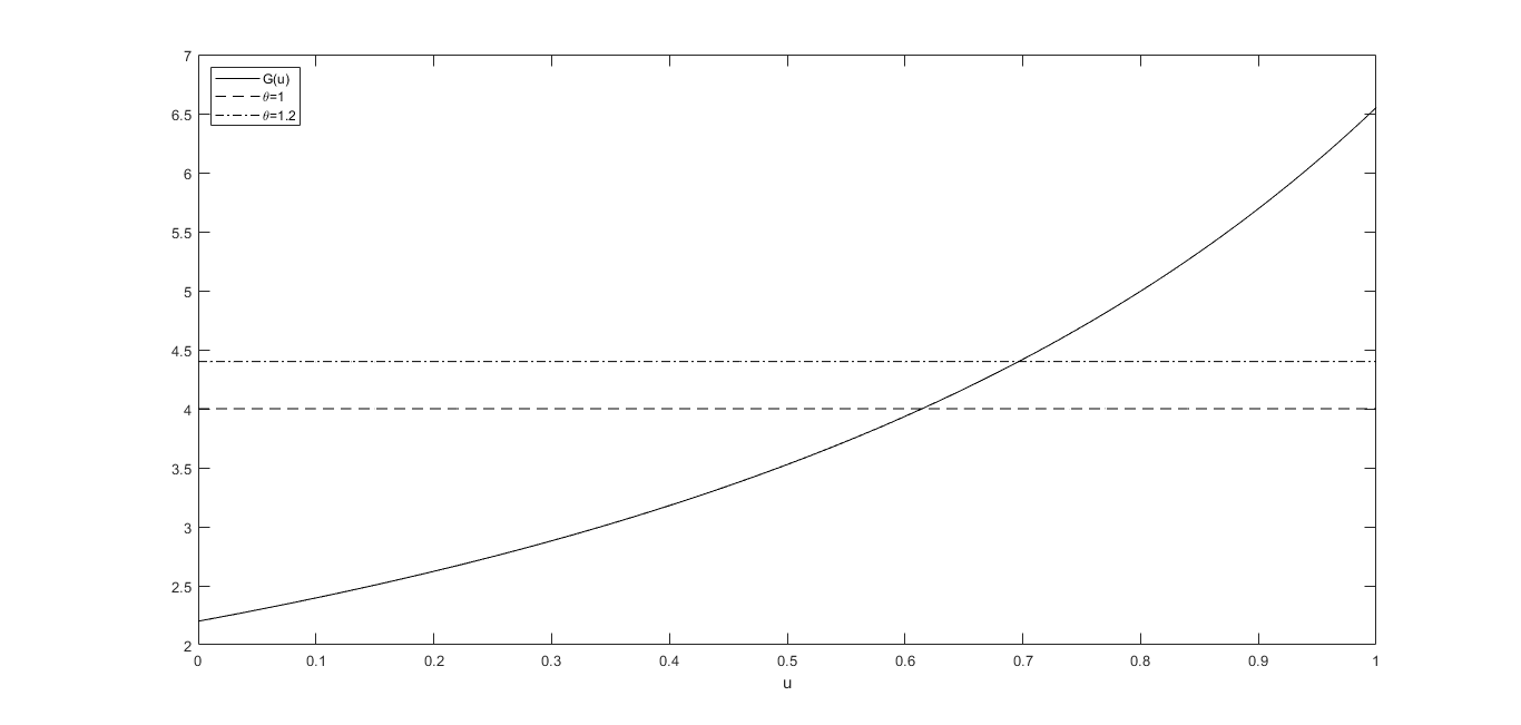
Figure 1: The effect of $\theta$ on the reinsurance strategy.

5.3.   Comparison with the case of complete information

In this subsection we compare the optimal strategy under partial information to the one with full information. In some special cases (see Propositions 5.3 and 5.4 below) we can prove that the optimal retention level under partial information is smaller than the one in the full information case. This means that the insurer who takes into account a partial information framework tends to buy an additional protection with respect to the (theoretical) case of complete information.

We consider the case of unknown time-homogeneous jump intensity (i.e. $\lambda(t,y)=\lambda(y)$) and known claims size distribution (i.e. $F_{Z}(t,y,dz)=F_{Z}(dz)$). Moreover, we suppose that the stochastic factor $Y$ takes value in a discrete set ${\cal S}=\{1,2,\dots\}$. Let us recall (see Remarks 2.6 and 2.7) that in this case the filter is described by the sequence $\pi_{t}(i)=P(Y_{t}=i|{\cal F}_{t}),i\in{\cal S}$ and $W(t,\pi_{t^{-}},z)=W(\pi_{t^{-}})=\{W_{i}(\pi_{t^{-}}),i\in{\cal S}\}$ by Eq. (2.23), where

$$W_{i}(\pi_{t^{-}})={\lambda(i)\pi_{t^{-}}(i)\over\sum_{j\in{\cal S}}\lambda(j)\pi_{t^{-}}(j)},\quad i\in{\cal S}.$$ (5.10)

Without loss of generality we assume $\lambda(1)\leq\lambda(2)\leq\dots$ and following the same lines as in [Liang and Bayraktar, 2014, Lemma 4.1] (where the case with a finite set ${\cal S}$ is discussed), see also [Bäuerle and Rieder, 2007, Theorem 5.6], we can prove that

$$v(t,W(\pi))\geq v(t,\pi),\quad\forall t\in[0,T],\pi\in\{\{\pi_{i}\}_{i\in{\cal S}};\quad\sum_{i\in{\cal S}}\pi_{i}=1,\pi_{i}\in[0,1]\}$$ (5.11)

with $W(\pi)=\{W_{i}(\pi),i\in{\cal S}\}$.

Proposition 5.3.

Let the assumptions of this subsection be satisfied. Under the proportional reinsurance and the premium calculation principles in Example 2.4, the optimal reinsurance strategy under partial information is always less or equal to the one under full information.

Proof.

We analyze two premium calculation principles and, correspondingly, we divide the proof in two parts.

Expected value principle

Under the expected value principle (see Eq. (2.17)) and a proportional reinsurance (i.e. $g(z,u)=uz,u\in[0,1]$ by Example 2.3), using Proposition 4.1 and Corollary 4.1 we easily obtain that the optimal reinsurance strategy is given by

$$u^{*}_{t}=\begin{cases}0&\text{if $1+\theta\leq\frac{v(t,W(\pi_{t^{-}}))}{v(t,\pi_{t^{-}})}$}\\ 1&\text{if $(1+\theta)\mathbb{E}[Z]\geq\int_{0}^{+\infty}\frac{v(t,W(\pi_{t^{-}}))}{v(t,\pi_{t^{-}})}ze^{\eta e^{R(T-t)}z}F_{Z}(dz)$ }\\ \hat{u}(t,\pi_{t^{-}})&\text{ otherwise,}\end{cases}$$ (5.12)

where $\hat{u}$ is the unique solution to

$$(1+\theta)\mathbb{E}[Z]=\frac{v(t,W(\pi_{t^{-}}))}{v(t,\pi_{t^{-}})}\int_{0}^{+\infty}ze^{\eta e^{R(T-t)}uz}F_{Z}(dz)\doteq h_{1}(t,\pi_{t^{-}},u).$$ (5.13)

In the full information case, from [Brachetta and Ceci, 2019b, Lemma 4.2], full reinsurance is never optimal, the optimal reinsurance strategy is a deterministic function of time and it is given by

$$u^{*,f}(t)=\begin{cases}1&\text{if $(1+\theta)\mathbb{E}[Z]\geq\int_{0}^{+\infty}ze^{\eta e^{R(T-t)}z}F_{Z}(dz)$}\\ \hat{u}^{f}(t)&\text{otherwise,}\end{cases}$$ (5.14)

where $\hat{u}^{f}$ is the unique solution to

$$(1+\theta)\mathbb{E}[Z]=\int_{0}^{+\infty}ze^{\eta e^{R(T-t)}uz}F_{Z}(dz)\doteq h_{0}(t,u)$$ (5.15)

Let us consider the equations (5.13) and (5.15) defined for all $u\in\mathbb{R}$, then equations (5.12) and (5.14) can be written as

$$u^{*}_{t}=0\land\hat{u}_{t}\lor 1\qquad\text{and}\qquad u^{*,f}(t)=\hat{u}^{f}(t)\lor 1,$$

respectively. Since

$$h_{1}(t,\pi_{t^{-}},u)=\frac{v(t,W(\pi_{t^{-}}))}{v(t,\pi_{t^{-}})}h_{0}(t,u)\geq h_{0}(t,u)\qquad\forall u\in[0,1],$$

and both sides are increasing in $u$, in order to have

$$h_{1}(t,\pi_{t^{-}},\hat{u}_{t})=1+\theta=h_{0}(t,\hat{u}^{f}(t)),$$

we must have that $\hat{u}_{t}\leq\hat{u}^{f}(t)$ (see Figure 2), which implies our statement.

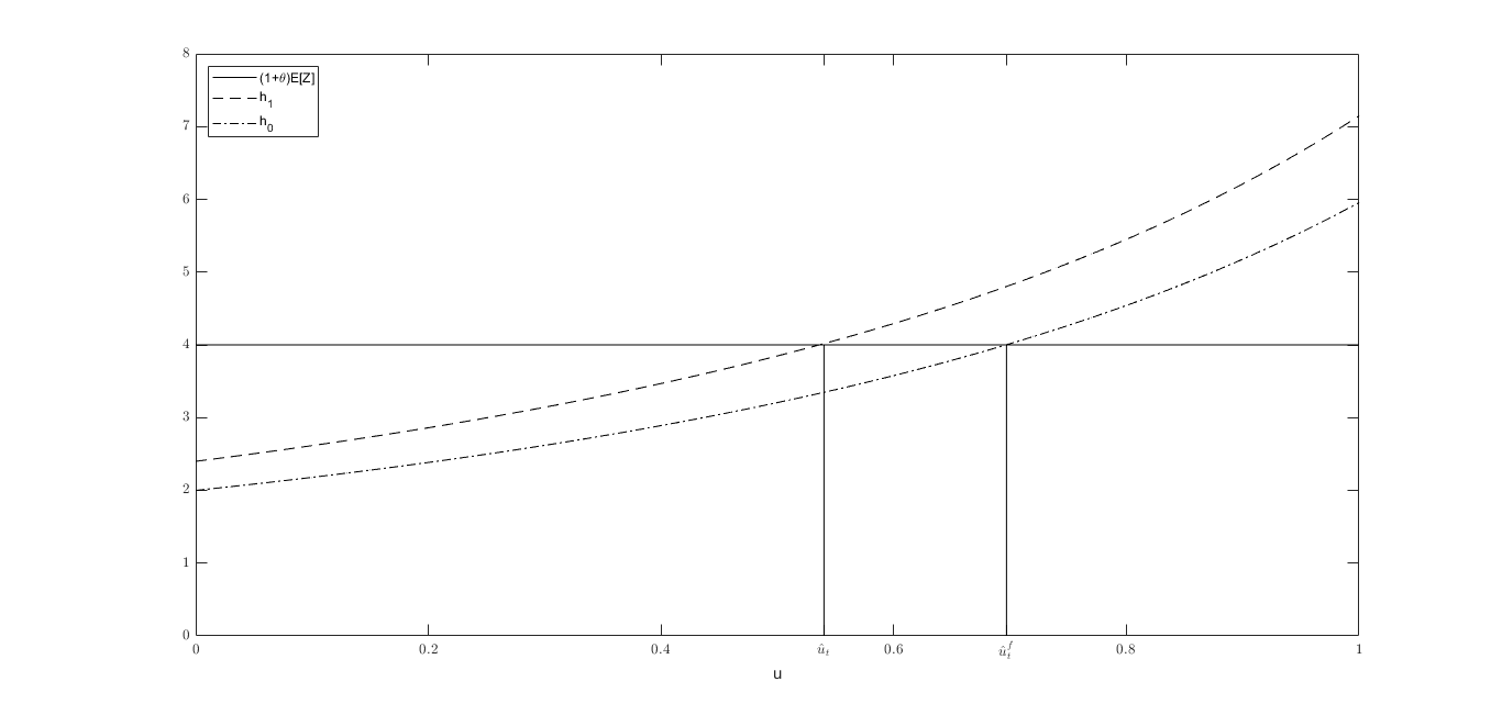
Figure 2: Functions $h_{1}$ and $h_{0}$ giving $\hat{u}_{t}$ and $\hat{u}^{f}(t)$ under the expected value principle.

Variance premium principle

Now let us denote

$$H(u)\doteq\mathbb{E}[Z]+2\theta(1-u)\mathbb{E}[Z^{2}].$$

By Corollary 4.1 we obtain that under the variance premium principle the optimal reinsurance strategy is given by

$$u^{*}_{t}=\begin{cases}0&\text{if $2\theta\mathbb{E}[Z^{2}]\leq(\frac{v(t,W(\pi_{t^{-}}))}{v(t,\pi_{t^{-}})}-1)\mathbb{E}[Z]$}\\ \hat{u}(t,\pi_{t^{-}})&\text{ otherwise,}\end{cases}$$ (5.16)

where $\hat{u}$ is the unique solution to

$$H(u)=h_{1}(t,\pi_{t^{-}},u).$$ (5.17)

In the full information case (see [Brachetta and Ceci, 2019b, Lemma 4.3]) the optimal strategy is a deterministic function of time and is given by $u^{*,f}(t)=\hat{u}^{f}(t)$, where $\hat{u}^{f}$ is the unique solution to

$$H(u)=h_{0}(t,u).$$

Hence the inequality $u^{*}_{t}\leq u^{*,f}(t)$ immediately follows by the same arguments as in the expected value principle case (see Figure 3).

Figure 3: Functions $h_{1}$ and $h_{0}$ giving $u^{*}_{t}$ and $u^{*,f}(t)$ under the variance premium principle.

∎

Proposition 5.4.

Let the assumptions of this subsection be satisfied and $F_{Z}(dz)$ admit density. Under the excess of loss reinsurance and the expected value principle the optimal reinsurance strategy is always less or equal to the one under full information.

Proof.

Consider the excess-of-loss reinsurance (see Example 2.3) and the expected value principle (see Eq. (2.17)). In the full information case, see [Brachetta and Ceci, 2019a, Proposition 8], the optimal reinsurance strategy satisfies

$$(1+\theta)(1-F_{Z}(u))=e^{\eta e^{R(T-t)}g(z,u))}(1-F_{Z}(u)),$$

so that it is given by

$$u^{*,f}(t)=\frac{1}{\eta}e^{-R(T-t)}\log(1+\theta).$$

In the partial information framework, taking into account Remark 4.2, Eq. (4.5) reads as

$$(1+\theta)(1-F_{Z}(u))=\frac{v(t,W(\pi_{t^{-}}))}{v(t,\pi_{t^{-}})}e^{\eta e^{R(T-t)}u}(1-F_{Z}(u)),$$

and we find out that

$$u^{*}_{t}=\frac{1}{\eta}e^{-R(T-t)}\log\Big{(}(1+\theta)\frac{v(t,\pi_{t^{-}})}{v(t,W(\pi_{t^{-}})}\Big{)}.$$

It is easy to see that $u^{*}_{t}\leq u^{*,f}(t)$ by the inequality (5.11). ∎

6.   Conclusions

This paper extends the existing results on optimal reinsurance in many directions. We introduce a general risk model where both the claims arrival intensity and the claim size distribution are affected by an environmental stochastic factor $Y$, which is modeled as a general Markov process (in [Liang and Bayraktar, 2014] it was a finite state Markov chain and in [Brachetta and Ceci, 2019a] a real-valued diffusion process). This model formulation allows the insurer to take into account risk fluctuations. However, it is well known that the insurer has only a partial information at disposal. Namely, she only observes the claims arrival times and the corresponding amount. Hence $Y$ is supposed to be unobservable and as a consequence claims arrival intensity and the claim size distribution has to be inferred from the observations. Considering general premium and reinsurance contract, we solve the optimization problem characterizing the value process and the optimal strategy in terms of a solution to a BSDE. Our results show that the insurer would react to risk fluctuations by modifying the reinsurance policy. Some examples for classical reinsurance agreements are illustrated. By analyzing the effect of safety loading on the optimal strategy we determine the price that the insurer deems reasonable for the reinsurer assuming part of her risks. Finally, we show that insurer with partial information is more conservative with respect the insurer with complete information.

Declaration of interest

None.

Appendix A Filtering with marked point processes observations

Here, we recall the main results on filtering with marked point processes observations. Under Assumption 2.4, the filter can be characterized as the unique strong solution of the so called Kushner-Stratonovich equation. We refer to [Ceci, 2006] and [Ceci and Colaneri, 2012] for a detailed proof.

Theorem A.1 (KS-equation).

Under Assumption 2.4, the filter $\pi$ is the unique strong solution to the Kushner-Stratonovich equation, for any bounded function $f\in\mathcal{D}^{Y}$

$$d\pi_{t}(f)=\pi_{t}(\mathcal{L}^{Y}f)dt+\int_{0}^{+\infty}w^{\pi}_{t}(f,z)(m(dt,dz)-\pi_{t^{-}}(\lambda F_{Z}(dz))dt),\quad\pi_{0}(f)=f(0,y_{0}),$$ (A.1)

where

$$w^{\pi}_{t}(f,z)\doteq\frac{d\pi_{t^{-}}(\lambda F_{Z}f)}{d\pi_{t^{-}}(\lambda F_{Z})}(z)-\pi_{t^{-}}(f)+\frac{d\pi_{t^{-}}({\bar{\cal L}}f)}{d\pi_{t^{-}}(\lambda F_{Z})}(z).$$ (A.2)

Here $\mathcal{\bar{L}}$ is an operator which takes into account possible common jump times between $Y$ and $m(dt,dz)$, while ${d\pi_{t^{-}}(\lambda F_{Z}f)\over d\pi_{t^{-}}(\lambda F_{Z})}(z)$ and ${d\pi_{t^{-}}(\mathcal{\bar{L}}f)\over d\pi_{t^{-}}(\lambda F_{Z})}(z)$ denote the Radon-Nikodym derivatives of the measures $\pi_{t^{-}}(\lambda F_{Z}(dz)f)$ and $\pi_{t^{-}}(\mathcal{\bar{L}}f(dz))$ with respect to $\pi_{t^{-}}(\lambda F_{Z}(dz))$, respectively.

The filtering equation has a natural recursive structure. In fact, between two consecutive jump times, $t\in(T_{n-1},T_{n})$, the equation reads as:

$$d\pi_{t}(f)=[\pi_{t}(\mathcal{L}^{0}f)+\pi_{t}(f)\pi_{t}(\lambda)-\pi_{t}(\lambda f)]dt,$$ (A.3)

where $\mathcal{L}^{0}f\doteq\mathcal{L}^{Y}f-\mathcal{\bar{L}}f$ and coincides with $\mathcal{L}^{Y}$ if there are not common jump times between state and observations.

At a jump time $T_{n}$:

$$\pi_{T_{n}}(f)={d\pi_{T_{n}^{-}}(\lambda F_{Z}f)\over d\pi_{T_{n}^{-}}(\lambda F_{Z})}(Z_{n})+{d\pi_{T_{n}^{-}}(\mathcal{\bar{L}}f)\over d\pi_{T_{n}^{-}}(\lambda F_{Z})}(Z_{n}).$$

Hence $\pi_{T_{n}}(f)$ is completely determined by the observed data $(T_{n},Z_{n})$ and by the knowledge of $\pi_{t}$ in the interval $t\in[T_{n-1},T_{n})$.

Let us observe that between two consecutive jump times the filter solves a non-linear deterministic equation (see Eq. (A.3)). We are able to provide a computable solution by means of a linearized method (see [Ceci and Gerardi, 2006, Lemma 3.1]). For simplicity, we assume no common jump times between $Y$ and $m(dt,dz)$ in the sequel.

Proposition A.1.

Let $\rho^{n}$ a process with values in the set of positive finite measures on $\mathbb{R}$ solution to the linear equation

$$d\rho^{n}_{t}(f)=\rho^{n}_{t}(\mathcal{L}^{Y}f-\lambda f)dt,\quad\rho^{n}_{T_{n-1}}(f)=\pi_{T_{n-1}}(f),\quad t\in(T_{n-1},T_{n}).$$

Then the process

$${\rho^{n}_{t}(f)\over\rho^{n}_{t}(1)},\qquad t\in(T_{n-1},T_{n}),$$

solves Eq. (A.3). Moreover the following representation holds

$$\rho^{n}_{t}(f)=E_{n-1}[f(t,Y_{t})e^{-\int_{s}^{t}\lambda(r,Y_{r})dr}]|_{s=T_{n-1}},$$

where $E_{n-1}$ denotes the conditional expectation given the distribution $Y_{T_{n-1}}$ equal to $\pi_{T_{n-1}}$.

Finally, Proposition 2.3 is a direct consequence of Proposition A.1 and of the strong uniqueness of solution to the Kushner-Stratonovich equation (A.1).

In the last part of the section we discuss same special cases.

Example A.1 (Known jump size distribution and unknown intensity).

Let $F_{Z}(t,y,dz)=F_{Z}(dz)$, then the filtering equation (A.3) reduces to

$$d\pi_{t}(f)=\pi_{t}(\mathcal{L}^{Y}f)dt+{\pi_{t^{-}}(\lambda f)-\pi_{t^{-}}(f)\pi_{t^{-}}(\lambda)\over\pi_{t^{-}}(\lambda)}(dN_{t}-\pi_{t^{-}}(\lambda)dt),$$

where $N_{t}=m((0,t]\times[0,+\infty))=\sum_{n\geq 1}\mathbbm{1}_{\{T_{n}\leq t\}}$ is the claims arrival process. Between two consecutive jump times, $t\in(T_{n-1},T_{n})$:

$$d\pi_{t}(f)=[\pi_{t}(\mathcal{L}^{Y}f)-\pi_{t}(\lambda f)+\pi_{t}(f)\pi_{t}(\lambda)]dt,$$

while at a jump time $T_{n}$:

$$\pi_{T_{n}}(f)=W(T_{n},\pi_{T_{n}^{-}})\doteq{\pi_{T_{n}^{-}}(\lambda f)\over\pi_{T_{n}^{-}}(\lambda)},$$

which coincides with Eq. (2.20) in Remark 2.6.

Example A.2 (Markov Modulated Risk Model with infinitely many states).

Now we consider the case where $Y$ is a continuous time Markov chain taking values in a discrete set ${\cal S}=\{1,2,\dots\}$ and $\{a_{ij}\}_{i\in{\cal S},j\in{\cal S}}$ its generator matrix. Here, $a_{ij}>0$, $i\neq j$, gives the intensity of a transition from state $i$ to state $j$, and it is such that $\sum_{j\geq 1,j\neq i}a_{ij}=-a_{ii}$. Defining the functions $f_{i}(y):=\mathbbm{1}_{y=i}$, $i\in{\cal S}$, the filter is completely described via the knowledge of $\pi_{t}(i):=\pi_{t}(f_{i})=P(Y_{t}=i\mid\mathcal{F}_{t})$, $i\in{\cal S}$, because for every function $f$ we have that

$$\pi_{t}(f)=\sum_{i\in{\cal S}}f(t,i)\pi_{t}(i).$$

The process $(\pi_{t}(i))_{i\in{\cal S}}$ is characterized via the following system of equations

$$d\pi_{t}(i)=\sum_{j\in{\cal S}}a_{ji}\pi_{t}(j)dt+\int_{0}^{+\infty}w^{\pi}_{t}(i,z)(m(dt,dz)-\sum_{j\in{\cal S}}\lambda(t,j)F_{Z}(t,j,dz)\pi_{t^{-}}(j)dt),\quad i\in{\cal S},$$ (A.4)

where

$$w^{\pi}_{t}(i,z)={d(\lambda(t,i)F_{Z}(t,i,dz)\pi_{t^{-}}(i))\over d(\sum_{j\in{\cal S}}\lambda(t,j)F_{Z}(t,j,dz)\pi_{t^{-}}(j))}(z)-\pi_{t^{-}}(i),$$

and we deduce Eq. (2.21) in Remark 2.6.
When $F_{Z}(t,i,dz)$ admits density $f_{Z}(t,i,z)$, $i\in{\cal S}$, it simplifies to

$$w^{\pi}_{t}(i,z)={\lambda(t,i)f_{Z}(t,i,z)\pi_{t^{-}}(i)\over\sum_{j\in{\cal S}}\lambda(t,j)f_{Z}(t,j,z)\pi_{t^{-}}(j)}-\pi_{t^{-}}(i).$$

In particular when ${\cal S}$ is a finite set, the system (A.4) is finite. This case has been considered in [Liang and Bayraktar, 2014], with the simplification of $\lambda(t,i)$ and $f_{Z}(t,j,z)$ not dependent on time.

Example A.3 (Markov Modulated Risk Model with known jump size distribution and unknown intensity).

In the special case where $F_{Z}(t,y,dz)=F_{Z}(dz)$, the system (A.4) reduces to

$$d\pi_{t}(i)=\sum_{j\in{\cal S}}a_{ji}\pi_{t}(j)dt+\Big{[}{\lambda(t,i)\pi_{t^{-}}(i)\over\sum_{j\in{\cal S}}\lambda(t,j)\pi_{t^{-}}(j)}-\pi_{t^{-}}(i)\Big{]}(dN_{t}-\sum_{j\in{\cal S}}\lambda(t,j)\pi_{t^{-}}(j)dt),\quad i\in{\cal S}.$$ (A.5)

Between two consecutive jump times, $t\in(T_{n-1},T_{n})$:

$$d\pi_{t}(f)=[\sum_{j\in{\cal S}}a_{ji}\pi_{t}(j)-\lambda(t,i)\pi_{t}(i)+\pi_{t}(i)\sum_{j\in{\cal S}}\lambda(t,j)\pi_{t}(j)]dt,$$

at a jump time $T_{n}$:

$$\pi_{T_{n}}(i)=W_{i}(T_{n},\pi_{T_{n}^{-}})\doteq{\lambda(T_{n},i)\pi_{T_{n}^{-}}(i)\over\sum_{j\in{\cal S}}\lambda(T_{n},j)\pi_{T_{n}^{-}}(j)}.$$

This latter formula provides Eq. (2.22) in Remark 2.6.
In particular when ${\cal S}$ is a finite set, the system (A.5) is finite.

References

- [Brachetta and Ceci, 2019a] Brachetta, M. and Ceci, C. (2019a). Optimal excess-of-loss reinsurance for stochastic factor risk models. Risks, 7(2).
- [Brachetta and Ceci, 2019b] Brachetta, M. and Ceci, C. (2019b). Optimal proportional reinsurance and investment for stochastic factor models. Insurance: Mathematics and Economics, 87:15 – 33.
- [Brémaud, 1981] Brémaud, P. (1981). Point Processes and Queues. Martingale dynamics. Springer-Verlag.
- [Bäuerle and Rieder, 2007] Bäuerle, N. and Rieder, U. (2007). Portfolio optimization with jumps and unobservable intensity process. Mathematical Finance, 17(2):205–224.
- [Ceci, 2004] Ceci, C. (2004). Optimal investment problems with marked point stock dynamics. In Progress in Probability, volume 63, pages 385–412. BirkhŁauser Verlag Basel/Switzerland.
- [Ceci, 2006] Ceci, C. (2006). Risk minimizing hedging for a partially observed high frequency data model. Stochastics, 78(1):13–31.
- [Ceci, 2012] Ceci, C. (2012). Utility maximization with intermediate consumption under restricted information for jump market models. International Journal of Theoretical and Applied Finance, 15(06):1250040.
- [Ceci and Colaneri, 2012] Ceci, C. and Colaneri, K. (2012). Nonlinear filtering for jump diffusion observations. Advances in Applied Probability, 44(3):678–701.
- [Ceci and Colaneri, 2014] Ceci, C. and Colaneri, K. (2014). The Zakai equation of nonlinear filtering for jump-diffusion observations: existence and uniqueness. Applied Mathematics and Optimization, 69(1):47–82.
- [Ceci and Gerardi, 2006] Ceci, C. and Gerardi, A. (2006). A model for high frequency data under partial information: a filtering approach. International Journal of Theoretical and Applied Finance, 9(4):555–576.
- [Ceci and Gerardi, 2011] Ceci, C. and Gerardi, A. (2011). Utility indifference valuation for jump risky assets. Decisions in Economics and Finance, 34(2):85–120.
- [Confortola and Fuhrman, 2013] Confortola, F. and Fuhrman, M. (2013). Backward stochastic differential equations and optimal control of marked point processes. SIAM J. Control and Optimization, 51:3592–3623.
- [Delong, 2013] Delong, L. (2013). Backward stochastic differential equations with jumps and their actuarial and financial applications. BSDEs with jumps.
- [El Karoui et al., 1997] El Karoui, N., Peng, S., and Quenez, M. C. (1997). Backward stochastic differential equations in finance. Mathematical Finance, 7(1):1–71.
- [Ethier and Kurtz, 1986] Ethier, S. and Kurtz, T. (1986). Markov Processes: Characterization and Convergence. John Wiley & Sons.
- [Grandell, 1991] Grandell, J. (1991). Aspects of risk theory. Springer-Verlag.
- [Irgens and Paulsen, 2004] Irgens, C. and Paulsen, J. (2004). Optimal control of risk exposure, reinsurance and investments for insurance portfolios. Insurance: Mathematics and Economics, 35:21–51.
- [Liang and Bayraktar, 2014] Liang, Z. and Bayraktar, E. (2014). Optimal reinsurance and investment with unobservable claim size and intensity. Insurance: Mathematics and Economics, 55:156–166.
- [Lim and Quenez, 2011] Lim, T. and Quenez, M.-C. (2011). Exponential utility maximization in an incomplete market with defaults. Electron. J. Probab., 16:1434–1464.
- [Liu and Ma, 2009] Liu, B. and Ma, J. (2009). Optimal reinsurance/investment problems for general insurance models. The Annals of Applied Probability, 19:1495–1528.
- [Rolski et al., 1999] Rolski, T., Schmidli, H., V., S., and Teugels, J. (1999). Stochastic processes for insurance and finance. Wiley.
- [Schmidli, 2008] Schmidli, H. (2008). Stochastic Control in Insurance. Springer-Verlag.
- [Schmidli, 2018] Schmidli, H. (2018). Risk Theory. Springer Actuarial. Springer International Publishing.
- [Young, 2006] Young, V. R. (2006). Premium principles. Encyclopedia of Actuarial Science, (3).