Variational Bethe Ansatz approach for dipolar one-dimensional bosons
Abstract
We propose a variational approximation to the ground state energy of a one-dimensional gas of interacting bosons on the continuum based on the Bethe Ansatz ground state wavefunction of the Lieb-Liniger model. We apply our variational approximation to a gas of dipolar bosons in the single mode approximation and obtain its ground state energy per unit length. This allows for the calculation of the Tomonaga-Luttinger exponent as a function of density and the determination of the structure factor at small momenta. Moreover, in the case of attractive dipolar interaction, an instability is predicted at a critical density, which could be accessed in lanthanide atoms.
I Introduction
One dimensional interacting bosonsCazalilla et al. (2011) are a very
active topic in current research on many-body problem, owing to
availability of experimental systems and powerful theoretical
techniques. One-dimensional bosons with repulsive interactions are
expected to have the Tomonaga-Luttinger liquid
stateHaldane (1981); Giamarchi (2004) as the ground
state, and display simultaneously critical superfluid and density
wave fluctuations with interaction dependent exponents. In contrast
to the case of fermionsGiamarchi (2004), these exponents cannot be obtained from
perturbation theory in the vicinity of the non-interacting
point. Instead, it is necessary to know the dependence of the
ground state energy per unit length as a function of particle
density.Haldane (1981) In the case of integrable
modelsLieb and Liniger (1963); Amico and
Korepin (2004) such
dependence can be obtained analytically, but in the general case,
one resorts to numerical methods such as Quantum Monte
CarloMazzanti et al. (2008); Citro et al. (2007) or Density
Matrix Renormalization
Group.Kühner and
Monien (1998) Variational methods
have also been proposedHellberg and Mele (1991); Kawakami and Horsch (1992); Hellberg and Mele (1992); Fradkin et al. (1993); Pham et al. (2000), using as variational
wavefunction the ground state wavefunction of the Calogero-Sutherland
model.Calogero (1969a, b); Sutherland (1971a, b, c) With
such variational wavefunctions, the Tomonaga-Luttinger exponent is
the variational parameter. This form of variational wavefunction can
be interpretedCapello et al. (2007) in terms of a
JastrowJastrow (1955) factor.
Because of the difficulty of computing
correlation functions, the use of Bethe Ansatz wavefunctions
as variational wavefunctions has been mainly restricted to few body
systemsRubeni et al. (2012); Wilson et al. (2014) in harmonic traps, although a Bethe Ansatz Density
Functional Theory has been proposed in the case of spin-1/2 fermions
in harmonic potential.Xianlong et al. (2006); Schenk et al. (2008) However,
Caux and
Maillet (2005); Caux and Calabrese (2006)
using determinant representations of correlation functions has allowed
calculation of the structure factor of Bethe Ansatz integrable
models. Such developments enable
the use of Bethe Ansatz wavefunctions in a variational
approach.Claeys et al. (2017) Moreover, in the case of the
integrable Lieb-LinigerLieb and Liniger (1963) gas, an
approximation to the exact structure factorCaux and Calabrese (2006) is
known, that further simplifies the variational calculation in the
thermodynamic limit.
Here we introduce a variational approach using the Bethe-Ansatz wavefunctions of the Lieb-Liniger model as variational wavefunctions to determine the Tomonaga-Luttinger exponents of a one-dimensional interacting model of bosons with a sufficiently short-range interaction. In particular, we apply it to a dipolar gas, using the separation of the dipole-dipole interaction(DDI) in an effective contact potential and a soft long-range part.
This study is particular timely as, recently, highly magnetic lanthanide atoms such as Dysprosium
and Erbium have given access to strong magnetic dipole-dipole
interactions (DDI) in ultracold
atomic physics .Lu et al. (2011, 2012); Aikawa et al. (2012, 2014) The interplay of the short-ranged
Van Der Waals s-wave interaction and the long-range and
anisotropy nature of DDI in the atomic gas has enabled the
exploration of a wide variety of phenomena. The most recent ones are novel quantum
liquids,Kadau et al. (2016); Chomaz et al. (2016); Ferrier-Barbut
et al. (2016) strongly correlated lattice states,de Paz et al. (2013, 2016); Baier et al. (2016)
exotic spin dynamicsNaylor et al. (2016) and the emergence of
thermalization in a nearly integrable quantum gas.Tang et al. (2018)
An even more exciting physics can be accessed when dimensionality is reduced. In fact in optical lattices, one would
be able to create dipolar Tomonaga-Luttinger liquidsSinha and Santos (2007); Citro et al. (2007)
as well as novel quantum phases,Yi et al. (2007) including analogs
of fractional quantum Hall states.Hafezi et al. (2007) On the application side, setting the DDI strength to zero
improves the sensitivity of atom interferometry,Fattori et al. (2008),
atomtronic devices based on dipolar interactions have been
proposedWittmann Wilsmann
et al. (2018), and tuning the interaction strength
from positive to negative may
find application in the simulation of nuclear matter.
Special attention has been devoted to the strictly one-dimensional case with repulsive interactions, in which both the determination of the equation of state Arkhipov et al. (2005) and of the structure factorCitro et al. (2008) has suggested the existence of a crossover from a liquid-like, superfluid state with the characteristics of a Tonks-Girardeau gas Girardeau (1960) to a quasi-ordered (particles localized at lattice sites), normal-fluid state with increasing the linear density. However, in trapped atom experiments, the finite transverse width of the trap allows an averaging of repulsive and attractive dipolar interactionsSinha and Santos (2007); Deuretzbacher et al. (2010) that precludes the formation of the quasi-ordered state. In the present paper, we wish to understand the crossover from the low density Tonks-Girardeau-like regime to the quasi-BEC regime at high density, by studying the evolution of the Tomonaga-Luttinger exponent with an approach applicable to interacting one-dimensional boson models in the continuum. Understanding the interplay between short-range Van Der Waals and longer ranged interactions remains an experimental challenge that may lead to new physics.
The paper is organized as follows. Section II describes the variational approach for a general setting. Section III introduces a model of dipolar bosons in a transverse harmonic trap,Sinha and Santos (2007); Deuretzbacher et al. (2010) and discusses the application of the variational approach and the computation of the Tomonaga-Luttinger parameters. In Section IV we offer some conclusions and perspectives.
II The variational approach
We consider the full Hamiltonian of a one-dimensional interacting bosonic system
| (1) |
where
with a sufficiently short ranged interaction, with Fourier transform , defined for all .
We then introduce the variational Hamiltonian:
| (2) |
where
which is a Lieb-Liniger Hamiltonian that is Bethe-Ansatz integrableLieb and Liniger (1963); Lieb (1963). Let the ground state wavefunction of the Lieb-Liniger Hamiltonian (2), such that .
We re-write the original Hamiltonian (1) in terms of the variational one as
| (3) |
and use as a variational wavefunction, so that is the variational energyClaeys et al. (2017) to be minimized as a function of
The Hellmann-Feynman theorem, , yields
| (4) |
We then express in terms of the static structure factor (see App. A for derivation and definitions) in the ground state and obtain the trial energy per unit length :
| (5) |
where is the number of bosons per unit length and is the Lieb-Liniger energy per unit length.
The calculation of the variational energy requires knowledge of and the static structure factor of the Lieb-Liniger model. The ground-state energy can be obtained from the Bethe Ansatz solutionLieb and Liniger (1963) by solving an integral equation (see App. B). It takes the form
| (6) |
with the dimensionless parameter
| (7) |
Moreover, an analytical conjecture for the exact result for is known,Lang et al. (2017); Ristivojevic (2019); Marino and Reis (2019) (see App. B) and can be readily used to estimate the derivative in Eq. (II). The static structure factor has been obtained from the form factor expansionCaux and Calabrese (2006), or using Monte Carlo approachesAstrakharchik and Giorgini (2003) for selected interaction strengths. Later, an analytic expression of , interpolating between weak and strong repulsion and in broad agreement with the result of Ref. Caux and Calabrese, 2006 was proposed.Cherny and Brand (2009) Using that approximation greatly simplifies the evaluation of the trial energy in Eq. (II). Once the optimal that minimizes the trial energy has been found, Eq. (II) yields an approximation for the ground state energy per unit length of the original Hamiltonian.
A one dimensional interacting system of spinless bosons with repulsive interactions is expected to form a Tomonaga-Luttinger liquid in its ground state.Cazalilla et al. (2011) The low-energy excitations of such Tomonaga-Luttinger liquid are described by a bosonized Hamiltonian
| (8) |
where is the velocity of excitations and the Tomonaga-Luttinger exponent. Haldane (1981) The latter exponent determines the long distance decay of the single particle Green’s function and of the density-density correlationsHaldane (1981) as well as the stability against the formation of a gapped state when an infinitesimal periodic potential commensurate with the density is applied along the tubes.Haller et al. (2010); Dalmonte et al. (2010); Boéris et al. (2016) The effect of renormalization of the Tomonaga-Luttinger exponent by a finite periodic potential on the phase diagram has been studied in Ref. Boéris et al., 2016. As a result of Galilean invarianceHaldane (1981) of (1),
| (9) |
whileHaldane (1981)
| (10) |
where is the ground state energy per unit length. The existence of the Tomonaga-Luttinger liquid requires . The vanishing of signals a collapse instabilityNakamura and Nomura (1997); Cabra and Drut (2003) towards a state of high (possibly infinite) density.
In the next section, we will illustrate the application of this variational method to a gas of one-dimensional dipolar bosons with repulsive contact interaction.
III The quasi-one dimensional dipolar model
The effective Hamiltonian in the single-mode approximation (SMA)Sinha and Santos (2007); Deuretzbacher et al. (2010), for polarized bosonic dipoles trapped in quasi-one dimensional geometry reads:
| (11) | |||||
where, compared to Hamiltonian (1) we have two contributions to the two-body potential energy: is the effective 1D dipole-dipole interaction obtained after projection of the transverse degrees of freedomSinha and Santos (2007); Deuretzbacher et al. (2010) and , which originates from the Van der Waals interaction and other short range interatomic interactions. These latter interactions are represented in three dimensions by the Huang-Yang pseudopotential.Huang and Yang (1957); Olshanii (1998) After projection of the transverse degrees of freedom, the pseudopotential yields the one-dimensional contact interaction withOlshanii (1998) where is the s-wave scattering length of the three-dimensional short range potential, is the transverse trapping length, and is a numerical constant. Away from the confinement induced resonance, , the single mode approximation is applicable, and one can approximate
| (12) |
If one wished to include confinement induced resonances, it would be necessary to include the Van der Waals and the dipolar interaction in a single Huang-Yang pseudopotential.Shi and Yi (2014) Such treatment is beyond the scope of our manuscript.
In the Hamiltonian Eq. (11), the effective 1D dipole-dipole interaction isSinha and Santos (2007); Deuretzbacher et al. (2010)
| (13) | |||
| (14) | |||
| (15) |
where is the magnetic permeability of the vacuum, is the magnetic dipolar moment of the atom ( in the caseTang et al. (2018) of 162Dy) and is the angle of the dipoles with respect to the -axis. The Fourier transform of the soft-dipolar interaction readsSinha and Santos (2007):
| (16) |
where is the exponential integral functionAbramowitz and Stegun (1972).
We can divide the Hamiltonian, Eq. (11), into a Lieb-Liniger part that contains all the contact interactions and the rest, a non-integrable soft-dipolar part. The Lieb-Liniger part of the Hamiltonian then reads:
where . The dimensionless parameter associated to is given by:
| (17) | |||||
where we have introduced the dipole length scale for the one dimensional dipolar interaction, as defined in Ref. Tang et al., 2015, which for the atoms is where is the Bohr radius. In the following, we will treat as a phenomenological parameter measuring the strength of the short range interaction. This value can be converted into a three-dimensional interaction using the approximation of Eq. (12).
The original Hamiltonian, Eq. (11), can therefore be written as the sum of the Lieb-Liniger part and the rest:
| (18) |
We can now use a variational Hamiltonian of the form Eq. (2), in which the contact interaction contains already the short range part of (11), and minimize the trial ground state energy (II). The variational contact interaction is written , with to be determined by minimization.
Following Sec. II, we can extract the optimal correction to by minimizing the trial energy per particle written in terms of dimensionless ratios and the adimensional parameter with respect to
| (19) | |||
where is dimensionless. Using for instance the golden search algorithm,Press et al. (1992) or simply scanning the energy as a function of it is possible to find the minimum of Eq. (19). The optimal , obtained through the minimization procedure, depends on three independent dimensionless parameters, such as , and . At the critical angle
| (20) |
the optimal coincides by construction with and depends only on . At large densities (see App. D) the contribution of the dipolar interactions in Eq. 19 is depressed by the factor together with the decay of , so that upon minimization asymptotically, as if the dipolar interaction was reduced to its contact contribution. If we consider Eq. (17) the contribution of the contact term due to dipolar interactions is independent of density , positive when and negative for , up to a point where can change its sign and become negative. In such a case, the Tomonaga-Luttinger liquid state should be unstable at high density. By contrast, for low densities, the non-contact contribution of the dipolar interactions to the variational energy is enhanced, and overwhelms the contact term. The optimal is enhanced when and lowered when (see App. C).
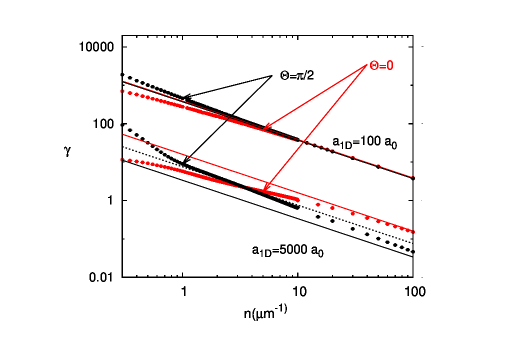
In Fig. 1 we show the dependence of (solid dots) on the density for two selected cases, and , and two angles, and . For comparison the value of (solid lines) from Eq. (17) are shown, as well as (dashed lines). When not stated explicitly all results refer to estimates where we have taken and .Tang et al. (2018)
In Ref. Tang et al., 2018, the dipolar interaction is approximated by replacing the full interaction (15) by where:
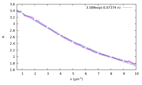
the integration bounds being chosen so that is 90% of the exact integral . Analogously to our variational approach the dipolar interaction is replaced by a simpler contact interaction. However, the criteria used to define the contact interaction are markedly different. In Ref. Tang et al., 2018, the potential is replaced by a -function potential having almost the same Fourier transform at . Such approximation is expected to be valid when the interparticle distance is large compared with , i.e. when . In our variational approach, no assumption is made on the two-particle scattering problem nor interparticle distance, since the effective contact interaction is determined by the minimization of the energy per particle. At low density, , it should be possible to make contact with the approximation of Ref.. Tang et al., 2018 and we should have
| (21) |
where is a dimensionless constant. The values of we find (see Fig. 2) are in reasonable agreement with the approximations used in Ref. Tang et al., 2018. However, the coefficient in Eq. (21) that gives the best fit to the variational value of decreases slightly with . In Fig. 3, we show the dependence of obtained by fitting the dependence of the optimal with an expression of the form (21). We find that the dependence can be described by an exponential, and that at low density the result of Ref. Tang et al., 2018 holds.

The minimum of the trial energy per particle, Eq. (19), in units of is , and can be expressed as
| (22) |
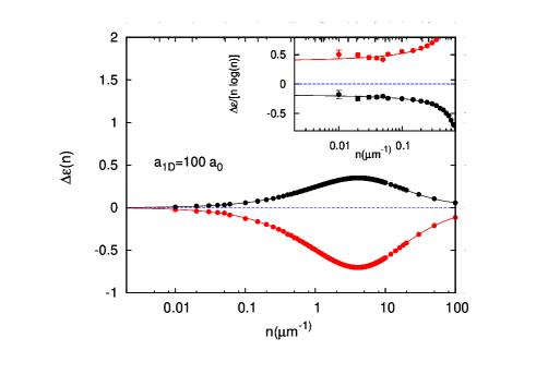
where is the dimensionless Lieb-Liniger ground-state energy defined in Eq. (6)) at dimensionless parameter (see Eq. (17)) while the contribution of the non-integrable soft-dipolar interaction is encapsulated in the correction.
As discussed before, at large density the and . At small density, whenever the optimal is so large that we can approximate the static structure factor as the one of the non-interacting fermionic gas, the correction due the soft dipolar interaction (see Appendix D for a detailed discussion). This behavior can be seen in Fig. 4 where the corrections are shown as a function of density for . At large density as well as for small density these corrections go to zero, in the inset we show that for extremely low density goes towards a constant value.
III.1 : repulsive soft dipolar interaction
As already observed, the overall effect of the repulsive soft dipolar interaction is to make the optimum . In the large density limit, , and according to Eq. (17), we can find if
| (23) |
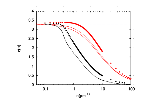
If that condition is satisfied, the dipolar gas is unstable at high density. Otherwise, the gas is stable for all densities. In Fig. 5 we show , together with , for various scattering length as a function of the density. At very low density the Tonks-Girardeau limit is recovered, while in the very high density limit the weakly interacting regime is recovered. The quantities and , solid and dashed lines in Fig. 5 respectively, can be seen as successive approximations to the variational energies (solid dots). In Fig. 5 we have also shown the case (, black data) where, for the parameters chosen to make the calculation, so the condition (23) is met. In the minimization procedure, for the densities considered, we always get a positive optimal .
III.2 : attractive soft dipolar interaction
When is negative, is enhanced by the contact contribution and the effect of the soft dipolar interaction is to lessen this repulsion. For small scattering lengths, the situation is similar to the one described for the repulsive case but with a negative correction with respect to in Eq. (22).
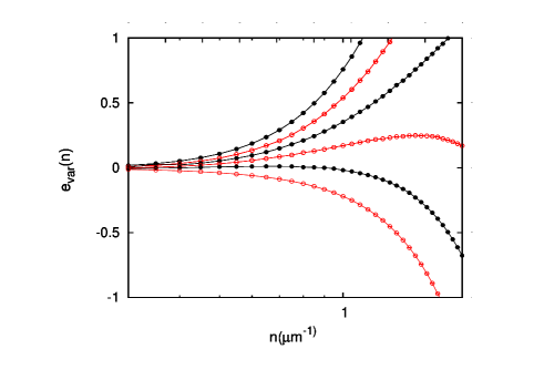
However for large scattering lengths at small angles, when the effect of the soft dipolar interaction is larger the system can become unstable. In Fig. 6 we show the variational ground state energy per unit length for different increasing scattering lengths. When the energy per unit length is convex at low density, but presents a concavity at higher density. In such case, the compressibility becomes negative, indicating an instability towards collapse at where the second derivative of energy per unit length as a function of density is vanishing.
III.3 Tomonaga-Luttinger parameters
Having obtained the ground state energy per unit length, with Eqs. (9-10) we can calculate the Tomonaga-Luttinger exponent as well as the velocity of excitations that enter the bosonized Hamiltonian Eq. (8).
At very low density the Tomonaga-Luttinger exponent has a logarithmic correction that qualitatively can be understood as follows (see also App. D). In the limit of low density, one can approximate
| (24) |
where we have used Eq. (46), giving
| (25) |
In the case of dipolar forcesDeuretzbacher et al. (2010), behaves for long distance distance as , so , leading to . This low density behavior can be traced in when minimizing the variational energy is sufficiently large to satisfy the above conditions. See for example Fig. 7, where obtained by fitting the low density behavior of the including a logarithmic correction (solid line) with an expression , is in agreement with the values obtained by numerical differentiation (open dots).
When the dipolar interaction is repulsive, the Tomonaga-Luttinger exponent is lower than the exponent of a Lieb-Liniger gas having either or minimizing the variational energy (19). This shows that the contribution from non-integrable soft dipolar interaction in (18) is not negligible, and that it is not correctly approximated by replacing the non-contact interaction in (18) by an effective contact interaction only.
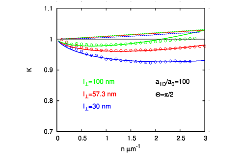
Moreover, such approximations always lead to a Tomonaga-Luttinger exponent larger than unity,Cherny and Brand (2009) and as we will see below, the dipolar gas can have a Tomonaga-Luttinger exponent less than unity. Reducing with fixed , while increases as . As the contribution to the ground-state energy is enhanced, the Tomonaga-Luttinger exponent is progressively reduced and for small density it can be less than unity like in the strictly one-dimensional dipolar gas dipolar gas.Citro et al. (2007); De Palo et al. (2008); Citro et al. (2008); Roscilde and Boninsegni (2010). In Fig. 7 we show for a fixed at , varying the confinement: namely and . This is a clear indication that approximating the Tomonaga-Luttinger exponent of the dipolar gas with the exponent of a Lieb-Liniger gas can lead to results incorrect not just quantitatively but also qualitatively. Indeed, finding a Tomonaga-Luttinger exponent yieldsGiamarchi (2004) , giving a cusp in near , whereas such cusp is absent with . However, the dynamical superfluid susceptibility remains divergent as long as .
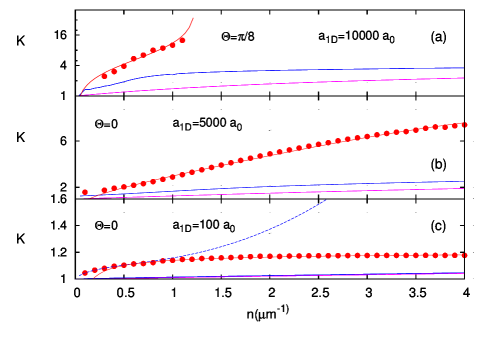
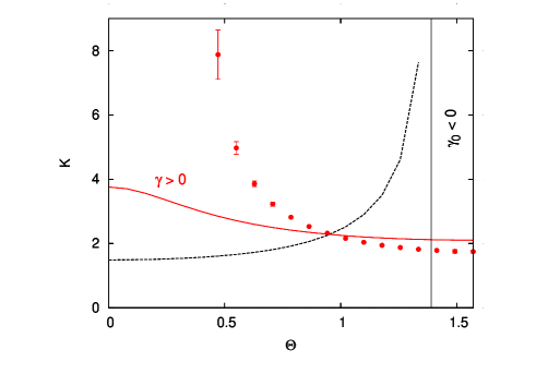
In the attractive case, the Tomonaga-Luttinger exponent, which is related to the compressibility by Eq. (10), diverges when the homogeneous ground state becomes unstable. In Fig. 8 in panel (a), for we show the case in which the system undergoes an instability with diverging at . Panels (b) and (c), for and respectively, show instead the enhancement of due the attractive interaction with respect to the approximations using the Tomonaga-Luttinger exponent of the Lieb-Liniger gas at the optimal or at . Moreover, when , the optimal corresponds to the Tonks-Girardeau limit (very low density), and the logarithmic correction to the exponent is visible ( see panel (c) where the blue dashed line is obtained by fitting the variational energy taking into account term, while a six degrees polynomial fit for the variational ground state energy gives results that do not match with the values of obtained with numerical differentiation). In Fig. 9 we follow the behavior of the Tomonaga-Luttinger exponent, at fixed density and fixed , as a function of the angle . This a case where the original is negative for large angles, while the optimal is positive in the whole range of . However corrections beyond predicts an instability for , as shown by the diverging corresponding to a change of sign in . While qualitatively, the Tomonaga-Luttinger exponent of a Lieb-Liniger gas with the optimal is a decreasing function of not showing any hint of instability. Moreover, the exponent that would be obtained by neglecting the non Lieb-Liniger part of Eq. (18) is an increasing function of and shows the instability for .
IV Conclusion
We have presented a variational approach to the ground state energy of bosons in the continuum interacting by a two-body potential, based on analytic expressions for the ground state energyLang et al. (2017) and structure factorCherny and Brand (2009) of the Lieb-Liniger model.
Using this variational approach we have calculated the ground-state energy bosonic atoms in transverse harmonic trapping with dipolar interactionTang et al. (2018) treated within the single mode approximation, as a function of density for several scattering lengths, confinement lengths and spanning the angle of dipoles. From the ground-state energy we have estimated the Tomonaga-Luttinger exponent as a function of density and interaction: when dipolar interactions are attractive and density is sufficiently high an instability of the Tomonaga-Luttinger liquid is predicted. Knowledge of the dependence of the variational ground state energy on the density will permit to consider the effect of longitudinal harmonic trapping, in particular to compute the frequencies of the breathing modes.Menotti and Stringari (2002); Fuchs et al. (2003, 2004); Oldziejewski et al. (2019) This will be the object of a future work. The variational method can be applied to other systems of interest such as atoms interacting via shoulder potentialsMattioli et al. (2013) or power law interactions.Douglas et al. (2015) The variational approach of the present paper could be extended in different directions. Since an exact form factor representation for the structure factorCaux and Calabrese (2006) of the Lieb-Liniger model is available, the the Tomonaga-Luttinger exponent and critical density could be calculated more accurately, albeit with greater computational cost with respect to the semi-analytical approach presented here. Second, the variational principle used here can be generalized to positive temperatureFeynman (1972) and the free energy of integrable models can be obtained from the Thermodynamic Bethe Ansatz.Yang and Yang (1969) Using form factor expansion techniques, the static structure factor of the Lieb-Liniger gas has been calculated for positive temperatures,Panfil and Caux (2014) thus the present variational approach could also be generalized to free energy calculations for positive temperatures.
Acknowledgements.
We thank B. Lev for discussions that inspired this project, and Z. Ristivojevic, L. Sanchez-Palencia, R. Oldziejewski for comments on the manuscript. E. O. thanks SISSA and Università di Trieste for hospitality.Appendix A Contributions to the variational energy
Writing explicitly the average by introducing and , being the number of particles and the system length, one has
| (26) |
where is the pair correlation function . In the integral (26), one can introduce the static structure factor with
| (27) |
where the relation is derived by the definition of the static structure factor:
| (28) |
so that the following relation between the static structure factor and the pair correlation function holds:
| (29) |
and hence:
| (30) |
where we have used the parity and .
The other contribution to the variational energy is evaluated using the Hellmann-Feynman theorem. One can show that in the Lieb-Liniger model,
| (31) |
where
| (32) |
Appendix B Ground state energy and static structure factor of the Lieb-Liniger gas
We can express the ground state energy as a function of the dimensionless parameter so that .
The function is given by the solution of integral equationsLieb and Liniger (1963)
| (33) | |||||
| (34) | |||||
| (35) |
where .
In our manuscript, instead of solving the integral equations (33)–(34) we will use the approximate analytical expression for the dimensionless energy suggested in Ref. Lang et al., 2017.
At small where the Lieb-Liniger energy is approximated by Lang et al. (2017)
| (36) | |||||
while from strong to intermediate coupling regimeLang et al. (2017)
| (37) | |||||
with . The expression (36) was obtainedLang et al. (2017) by fitting the ground state energy to a polynomial expression in for . An exact expansion has been conjecturedRistivojevic (2019); Marino and Reis (2019). We have checked that in the range the relative difference between the two expressions was under , while the relative difference between the derivatives was under . Using the expansionRistivojevic (2019); Marino and Reis (2019) instead of Eq. (36)in the variational calculation of the ground state energy yields relative differences under . Concerning the expression (37), we note that an alternative asymptotic expansionRistivojevic (2014); Lang (2019) in powers of also applies for . However, the expression (37) is more convenientLang et al. (2017) to match with (36) in the intermediate region of .
Using the phenomenological suggestion given in Ref. Cherny and Brand, 2009 for structure factor it is possible to have an approximate estimate of the static structure factor in terms of ratio between Gauss hypergeometric functionsAbramowitz and Stegun (1972)
| (38) |
where is the Tomonaga-Luttinger exponent, is the dispersion of the Type-I Lieb excitationsLieb (1963), the dispersion of the Type-II Lieb excitationsLieb (1963) for and otherwise, and are the exponents of the threshold singularity respectively at and can be calculated from the shift function.Khodas et al. (2007); Imambekov and Glazman (2009); Cherny and Brand (2009) The expression (38) reduces to Eq. (22) in Ref. Cherny and Brand, 2009 when the approximation is made.

To calculate we have to considerCherny and Brand (2009) the integral equation for the shift function:
| (39) |
and
| (40) | |||
| (41) |
Then, the dispersion of Lieb modes is given by:
| (42) |
for type I, and
| (43) |
with for type-II. When , Eq.(B) reduces, up to a sign, to the dispersion of the Lieb-I mode shifted of . For a given wavevector , one must first determine that solves , and calculate to obtain the dispersionLieb (1963); Cherny and Brand (2009). Once is known, the quantities
| (44) |
are found from the integral equation (B), and the threshold exponent of the Lieb-I modeKhodas et al. (2007); Imambekov and Glazman (2009) is
| (45) |
Similarly, having found , one obtains by replacing with in (44). Substituting with in Eq.(B), the threshold singularity exponent of the dynamical structure factor at the lower edge is found.Khodas et al. (2007); Cherny and Brand (2009); Imambekov and Glazman (2009) For , the lower edge is given by the Lieb-II mode, while for it is given by a replica of the Lieb-I mode shifted by .
In the limit of , the exact expression of simplifies to
| (46) |
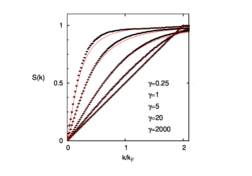
In some selected cases, from Quantum Monte Carlo simulations can be used as benchmark for expression (38) ; comparison between the static structure factor from simulations and from the approximated Ansatz,for some selected cases, are shown in Fig. 11. The linear increase for small predicted by bosonizationCitro et al. (2007) is well reproduced by both simulations and the Ansatz (38). The agreement between simulations and Ansatz is better for the case of . We note that in Ref. Cherny and Brand, 2009, a satisfactory comparison with the expression obtained for form factor summation was already shown.
Appendix C minimization of the energy
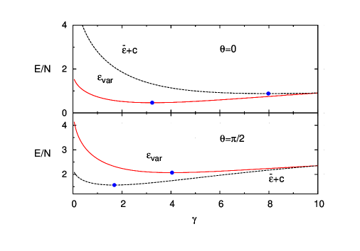
In Fig. 12 we show Eq. (19) with and without the dipolar interaction term, for and , for when the interaction is maximally attractive and for where when the interaction is maximally repulsive. When the dipolar interaction is repulsive it enhances the total repulsion and hence the optimal value of its greater than , whereas when it is attractive it reduces the total repulsion so that the optimal .
Appendix D high and low density limits of the variational energy
Analytic expressions of can be obtained using the Lieb-Liniger ground state energy derived in Lang et al. (2017) and the expressions of the structure factor derived in Cherny and Brand (2009) for and for . In the latter case, using (24), we have
| (47) |
and using (9)– (10) the Tomonaga-Luttinger exponent is given by
| (48) |
so that in the limit , , the expected behavior with interactions decaying as at long distance. In the case of , we can approximateCherny and Brand (2009)
| (49) |
leading to a variational energy
| (50) | |||||
Minimizing with respect to , we obtain
| (51) |
where we have defined
| (52) |
References
- Cazalilla et al. (2011) M. A. Cazalilla, R. Citro, T. Giamarchi, E. Orignac, and M. Rigol, Rev. Mod. Phys. 83, 1405 (2011).
- Haldane (1981) F. D. M. Haldane, Phys. Rev. Lett. 47, 1840 (1981).
- Giamarchi (2004) T. Giamarchi, Quantum Physics in One Dimension (Oxford University Press, Oxford, 2004).
- Lieb and Liniger (1963) E. H. Lieb and W. Liniger, Phys. Rev. 130, 1605 (1963).
- Amico and Korepin (2004) L. Amico and V. Korepin, Ann. Phys. (N. Y.) 314, 496 (2004).
- Mazzanti et al. (2008) F. Mazzanti, G. E. Astrakharchik, J. Boronat, and J. Casulleras, Phys. Rev. A 77, 043632 (2008), arXiv:0712.3593v1.
- Citro et al. (2007) R. Citro, E. Orignac, S. De Palo, and M.-L. Chiofalo, Phys. Rev. A 75, 051602(R) (2007), eprint cond-mat/0611667.
- Kühner and Monien (1998) T. D. Kühner and H. Monien, Phys. Rev. B 58, R14741 (1998).
- Hellberg and Mele (1991) C. S. Hellberg and E. J. Mele, Phys. Rev. Lett. 67, 2080 (1991).
- Kawakami and Horsch (1992) N. Kawakami and P. Horsch, Phys. Rev. Lett. 68, 3110 (1992).
- Hellberg and Mele (1992) C. S. Hellberg and E. J. Mele, Phys. Rev. Lett. 68, 3111 (1992).
- Fradkin et al. (1993) E. Fradkin, E. Moreno, and F. A. Schaposnik, Nucl. Phys. B 392, 667 (1993), eprint hep-th/9207003.
- Pham et al. (2000) K. V. Pham, M. Gabay, and P. Lederer, Phys. Rev. B 61, 16397 (2000).
- Calogero (1969a) F. Calogero, J. Math. Phys. 10, 2191 (1969a).
- Calogero (1969b) F. Calogero, J. Math. Phys. 10, 2197 (1969b).
- Sutherland (1971a) B. Sutherland, J. Math. Phys. 12, 246 (1971a).
- Sutherland (1971b) B. Sutherland, J. Math. Phys. 12, 251 (1971b).
- Sutherland (1971c) B. Sutherland, Phys. Rev. A 4, 2019 (1971c).
- Capello et al. (2007) M. Capello, F. Becca, M. Fabrizio, and S. Sorella, Phys. Rev. Lett. 99, 056402 (2007), eprint arXiv:0705.2684.
- Jastrow (1955) R. Jastrow, Phys. Rev. 98, 1479 (1955).
- Rubeni et al. (2012) D. Rubeni, A. Foerster, and I. Roditi, Phys. Rev. A 86, 043619 (2012).
- Wilson et al. (2014) B. Wilson, A. Foerster, C. Kuhn, I. Roditi, and D. Rubeni, Phys. Lett. A 378, 1065 (2014).
- Xianlong et al. (2006) G. Xianlong, M. Polini, M. Tosi, V. L. Campo, Jr., K. Capelle, and M. Rigol, Phys. Rev. B 73, 165120 (2006), cond-mat/0512184.
- Schenk et al. (2008) S. Schenk, M. Dzierzawa, P. Schwab, and U. Eckern, Phys. Rev. B 78, 165102 (2008).
- Caux and Maillet (2005) J.-S. Caux and J.-M. Maillet, Phys. Rev. Lett. 95, 077201 (2005), cond-mat/0502365.
- Caux and Calabrese (2006) J.-S. Caux and P. Calabrese, Phys. Rev. A 74, 031605(R) (2006), eprint arXiv:cond-mat/0603654.
- Claeys et al. (2017) P. W. Claeys, J.-S. Caux, D. Van Neck, and S. De Baerdemacker, Phys. Rev. B 96, 155149 (2017), URL https://link.aps.org/doi/10.1103/PhysRevB.96.155149.
- Lu et al. (2011) M. Lu, N. Q. Burdick, S. H. Youn, and B. L. Lev, Phys. Rev. Lett. 107, 190401 (2011), URL https://link.aps.org/doi/10.1103/PhysRevLett.107.190401.
- Lu et al. (2012) M. Lu, N. Q. Burdick, and B. L. Lev, Phys. Rev. Lett. 108, 215301 (2012), URL https://link.aps.org/doi/10.1103/PhysRevLett.108.215301.
- Aikawa et al. (2012) K. Aikawa, A. Frisch, M. Mark, S. Baier, A. Rietzler, R. Grimm, and F. Ferlaino, Phys. Rev. Lett. 108, 210401 (2012), URL https://link.aps.org/doi/10.1103/PhysRevLett.108.210401.
- Aikawa et al. (2014) K. Aikawa, A. Frisch, M. Mark, S. Baier, R. Grimm, and F. Ferlaino, Phys. Rev. Lett. 112, 010404 (2014), URL https://link.aps.org/doi/10.1103/PhysRevLett.112.010404.
- Kadau et al. (2016) H. Kadau, M. Schmitt, M. Wenzel, C. Wink, T. Maier, I. Ferrier-Barbut, and T. Pfau, Nature 530, 194 (2016), URL https://doi.org/10.1038/nature16485.
- Chomaz et al. (2016) L. Chomaz, S. Baier, D. Petter, M. J. Mark, F. Wächtler, L. Santos, and F. Ferlaino, Phys. Rev. X 6, 041039 (2016), URL https://link.aps.org/doi/10.1103/PhysRevX.6.041039.
- Ferrier-Barbut et al. (2016) I. Ferrier-Barbut, H. Kadau, M. Schmitt, M. Wenzel, and T. Pfau, Phys. Rev. Lett. 116, 215301 (2016), URL https://link.aps.org/doi/10.1103/PhysRevLett.116.215301.
- de Paz et al. (2013) A. de Paz, A. Sharma, A. Chotia, E. Maréchal, J. H. Huckans, P. Pedri, L. Santos, O. Gorceix, L. Vernac, and B. Laburthe-Tolra, Phys. Rev. Lett. 111, 185305 (2013), URL https://link.aps.org/doi/10.1103/PhysRevLett.111.185305.
- de Paz et al. (2016) A. de Paz, P. Pedri, A. Sharma, M. Efremov, B. Naylor, O. Gorceix, E. Maréchal, L. Vernac, and B. Laburthe-Tolra, Phys. Rev. A 93, 021603(R) (2016), URL https://link.aps.org/doi/10.1103/PhysRevA.93.021603.
- Baier et al. (2016) S. Baier, M. J. Mark, D. Petter, K. Aikawa, Z. C. L. Chomaz, M. Baranov, P. Zoller, and F. Ferlaino, Science 352, 201 (2016).
- Naylor et al. (2016) B. Naylor, M. Brewczyk, M. Gajda, O. Gorceix, E. Marechal, L. Vernac, and B. Laburthe-Tolra, Phys. Rev. Lett. 117, 185302 (2016).
- Tang et al. (2018) Y. Tang, W. Kao, K.-Y. Li, S. Seo, K. Mallayya, M. Rigol, S. Gopalakrishnan, and B. L. Lev, Phys. Rev. X 8, 021030 (2018), arXiv: 1707.07031, URL http://arxiv.org/abs/1707.07031.
- Sinha and Santos (2007) S. Sinha and L. Santos, Phys. Rev. Lett. 99, 140406 (2007).
- Yi et al. (2007) S. Yi, T. Li, and C. P. Sun, Phys. Rev. Lett. 98, 260405 (2007), URL https://link.aps.org/doi/10.1103/PhysRevLett.98.260405.
- Hafezi et al. (2007) M. Hafezi, A. S. Sørensen, E. Demler, and M. D. Lukin, Phys. Rev. A 76, 023613 (2007), URL https://link.aps.org/doi/10.1103/PhysRevA.76.023613.
- Fattori et al. (2008) M. Fattori, G. Roati, B. Deissler, C. D’Errico, M. Zaccanti, M. Jona-Lasinio, L. Santos, M. Inguscio, and G. Modugno, Phys. Rev. Lett. 101, 190405 (2008), URL https://link.aps.org/doi/10.1103/PhysRevLett.101.190405.
- Wittmann Wilsmann et al. (2018) K. Wittmann Wilsmann, L. H. Ymai, A. P. Tonel, J. Links, and A. Foerster, Commun. Phys. 1, 1 (2018).
- Arkhipov et al. (2005) A. S. Arkhipov, G. E. Astrakharchik, A. V. Belikov, and Y. E. Lozovik, JETP Lett. 82, 39 (2005).
- Citro et al. (2008) R. Citro, S. De Palo, E. Orignac, P. Pedri, and M. Chiofalo, New J. Phys. 10, 045011 (2008).
- Girardeau (1960) M. Girardeau, J. Math. Phys. 1, 516 (1960).
- Deuretzbacher et al. (2010) F. Deuretzbacher, J. C. Cremon, and S. M. Reimann, Phys. Rev. A 81, 063616 (2010), [Erratum: Phys. Rev. A 87, 039903(E) (2013)], URL https://link.aps.org/doi/10.1103/PhysRevA.81.063616.
- Lieb (1963) E. H. Lieb, Phys. Rev. 130, 1616 (1963).
- Lang et al. (2017) G. Lang, F. Hekking, and A. Minguzzi, SciPost Phys. 3, 003 (2017), URL https://scipost.org/10.21468/SciPostPhys.3.1.003.
- Ristivojevic (2019) Z. Ristivojevic, Phys. Rev. B 100, 081110 (2019).
- Marino and Reis (2019) M. Marino and T. Reis, J. Stat. Phys. 177, 1148 (2019), arXiv:1905.09575.
- Astrakharchik and Giorgini (2003) G. E. Astrakharchik and S. Giorgini, Phys. Rev. A 68, 031602 (2003), URL https://link.aps.org/doi/10.1103/PhysRevA.68.031602.
- Cherny and Brand (2009) A. Cherny and J. Brand, Phys. Rev. A 79, 043607 (2009).
- Haller et al. (2010) E. Haller, R. Hart, M. J. Mark, J. G. Danzl, L. Reichsöllner, M. Gustavsson, M. Dalmonte, G. Pupillo, and H.-C. Nägerl, Nature (London) 466, 597 (2010).
- Dalmonte et al. (2010) M. Dalmonte, G. Pupillo, and P. Zoller, Phys. Rev. Lett. 105, 140401 (2010).
- Boéris et al. (2016) G. Boéris, L. Gori, M. D. Hoogerland, A. Kumar, E. Lucioni, L. Tanzi, M. Inguscio, T. Giamarchi, C. D’Errico, G. Carleo, et al., Phys. Rev. A 93, 011601 (2016), URL https://link.aps.org/doi/10.1103/PhysRevA.93.011601.
- Nakamura and Nomura (1997) M. Nakamura and K. Nomura, Phys. Rev. B 56, 12840 (1997).
- Cabra and Drut (2003) D. C. Cabra and J. E. Drut, J. Phys.: Condens. Matter 15, 1445 (2003).
- Huang and Yang (1957) K. Huang and C. N. Yang, Phys. Rev. 105, 767 (1957).
- Olshanii (1998) M. Olshanii, Phys. Rev. Lett. 81, 938 (1998).
- Shi and Yi (2014) T. Shi and S. Yi, Phys. Rev. A 90, 042710 (2014).
- Abramowitz and Stegun (1972) M. Abramowitz and I. Stegun, eds., Handbook of mathematical functions (Dover, New York, 1972).
- Tang et al. (2015) Y. Tang, A. Sykes, N. Q. Burdick, J. L. Bohn, and B. L. Lev, Phys. Rev. A 92, 022703 (2015), URL https://link.aps.org/doi/10.1103/PhysRevA.92.022703.
- Press et al. (1992) W. H. Press, S. A. Teukolsky, W. T. Vetterling, and B. P. Flannery, Numerical Recipes in Fortran : the art of scientific computing (Cambridge University Press, Cambridge, UK, 1992), chap. 10, p. 390.
- De Palo et al. (2008) S. De Palo, E. Orignac, R. Citro, and M. L. Chiofalo, Phys. Rev. B 77, 212101 (2008), eprint arXiv:0801.1200.
- Roscilde and Boninsegni (2010) T. Roscilde and M. Boninsegni, New J. Phys. 12, 033032 (2010).
- Menotti and Stringari (2002) C. Menotti and S. Stringari, Phys. Rev. A 66, 043610 (2002).
- Fuchs et al. (2003) J. N. Fuchs, X. Leyronas, and R. Combescot, Phys. Rev. A 68, 043610 (2003), eprint cond-mat/0305647.
- Fuchs et al. (2004) J. Fuchs, X. Leyronas, and R. Combescot, Laser Physics 14, 1 (2004).
- Oldziejewski et al. (2019) R. Oldziejewski, W. Górecki, K. Pawlowski, and K. Rzazewski, Strongly correlated quantum droplets in quasi-1d dipolar Bose gas (2019), arXiv:1908.00108, URL http://arxiv.org/abs/1908.00108.
- Mattioli et al. (2013) M. Mattioli, M. Dalmonte, W. Lechner, and G. Pupillo, Phys. Rev. Lett. 111, 165302 (2013).
- Douglas et al. (2015) J. S. Douglas, H. Habibian, C. L. Hung, A. V. Gorshkov, H. J. Kimble, and D. E. Chang, Nature Photonics 9, 326 (2015), eprint arXiv:1312.2435.
- Feynman (1972) R. P. Feynman, Statistical Mechanics (Benjamin, Reading, MA, 1972).
- Yang and Yang (1969) C. N. Yang and C. P. Yang, J. Math. Phys. 10, 1115 (1969).
- Panfil and Caux (2014) M. Panfil and J.-S. Caux, Phys. Rev. A 89, 033605 (2014), eprint 1308.2887.
- Ristivojevic (2014) Z. Ristivojevic, Phys. Rev. Lett. 113, 015301 (2014).
- Lang (2019) G. Lang, SciPost Phys. 7, 55 (2019), arXiv:1907.04410.
- Khodas et al. (2007) M. Khodas, M. Pustilnik, A. Kamenev, and L. I. Glazman, Phys. Rev. Lett. 99, 110405 (2007).
- Imambekov and Glazman (2009) A. Imambekov and L. I. Glazman, Phys. Rev. Lett. 102, 126405 (2009).