Generalized space-time fractional dynamics in networks and lattices

Abstract

We analyze generalized space-time fractional motions on undirected networks and lattices. The continuous-time random walk (CTRW) approach of Montroll and Weiss is employed to subordinate a space fractional walk to a generalization of the time-fractional Poisson renewal process. This process introduces a non-Markovian walk with long-time memory effects and fat-tailed characteristics in the waiting time density. We analyze ‘generalized space-time fractional diffusion’ in the infinite $\it d$-dimensional integer lattice $\it\mathbb{Z}^{d}$. We obtain in the diffusion limit a ‘macroscopic’ space-time fractional diffusion equation. Classical CTRW models such as with Laskin’s fractional Poisson process and standard Poisson process which occur as special cases are also analyzed. The developed generalized space-time fractional CTRW model contains a four-dimensional parameter space and offers therefore a great flexibility to describe real-world situations in complex systems.

1 INTRODUCTION

Random walk models are considered to be the most fundamental approaches to describe stochastic processes in nature. Hence applications of random walks cover a very wide area in fields as various as random search strategies, the proliferation of plant seeds, the spreading phenomena of pandemics or pollution, chemical reactions, finance, population dynamics, properties of public transportation networks, anomalous diffusion and generally such approaches are able to capture empirically observed power-law features in ‘complex systems’ [1, 2, 3, 4, 5, 6, 7]. On the other hand the emergence of “network science”, and especially the study of random walks on networks has become a major subject for the description of dynamical properties in complex systems [8, 9, 10].

In classical random walks in networks, the so-called ‘normal random walks’, the walker in one step can reach only connected next neighbor sites [11, 12]. To the class of classical Markovian walks refer continuous-time random walks (CTRWs) where the walker undertakes jumps from one node to another where the waiting time between successive jumps are exponentially distributed leading to Poisson distributed numbers of jumps. The classical CTRW models with Poisson renewal process are able to capture normal diffusive properties such as the linear increase of the variance of a diffusing particle [6]. However, these classical walks are unable to describe power-law features exhibited by many complex systems such as the sublinear time characteristics of the mean-square displacement in anomalous diffusion [5]. It has been demonstrated that such anomalous diffusive behavior is well described by a random walk subordinated to the fractional generalization of the Poisson process. This process which was to our knowledge first introduced by Repin and Saichev [13], was developed and analyzed by Laskin who called this process the ‘fractional Poisson process’ [14, 15]. The Laskin’s fractional Poisson process was further generalized in order to obtain greater flexibility to adopt real-world situations [16, 17, 18]. We refer this renewal process to as ‘generalized fractional Poisson process’ (GFPP). Recently we developed a CTRW model of a normal random walk subordinated to a GFPP [17, 18].

The purpose of the present paper is to explore space fractional random walks that are subordinated to a GFPP. We analyze such motions in undirected networks and as a special application in the multidimensional infinite integer lattice $\it\mathbb{Z}^{d}$.

2 RENEWAL PROCESS AND CONTINUOUS-TIME RANDOM WALK

In the present section, our aim is to give a brief outline of renewal processes (or also referred to as ‘compound processes’) and closely related to the ‘continuous-time random walk (CTRW)’ approach which was introduced by Montroll and Weiss [19]. For further outline of renewal theory and related subjects we refer to the references [2, 4, 19, 20, 21, 22]. It is mention worthy that we deal in this paper with causal generalized functions and distributions in the sense of Gelfand and Shilov [23].

We consider a sequence of randomly occurring ‘events’. Such events can be for instance the jumps of a diffusing particle or failure events in technical systems. We assume that the events occur at non-negative random times $\it 0\leq t_{1},t_{2},\ldots t_{n},\ldots,\infty$ where $t=0$ represents the start of the observation. The random times $t_{k}$ when events occur are called ‘arrival times’. The time intervals between successive events $\it\Delta t_{k}=t_{k}-t_{k-1}\geq 0$ are called ‘waiting times’ or ‘interarrival times’ [20]. The random event stream is referred to as a renewal process if the waiting time $\it\Delta t$ between successive events is an ‘independent and identically distributed’ (IID) random variable which may take any non-negative continuous value. This means in a renewal process the waiting time $\it\Delta t_{k}$ between successive events is drawn $\it\forall k$ from the same waiting probability density function (PDF) $\it\chi(t)$. This distribution function is called waiting time distribution function (waiting time PDF) or short waiting time density. The quantity $\it\chi(t){\rm d}t$ indicates the probability that an event occurs at time $\it t$ (within $\it[t,t+{\rm d}t]$).

We can then write the probability $\it\Psi(t)$ that the waiting time for the first event is $\it\Delta t\leq t$ or equivalently that at least one event occurs in the time interval $\it[0,t]$ as

$$\it\Psi(t)=\int_{0}^{t}\chi(\tau){\rm d}\tau,\hskip 14.22636ptt\geq 0,\hskip 14.22636pt\lim_{t\rightarrow\infty}\Psi(t)=1-0$$ (1)

with the obvious initial condition $\it\Psi(t=0)=0$. The distribution (1) in the context of lifetime models often is also called ‘failure probability’ [20]. From this relation follows that the waiting time density $\it\chi(t)$ is a normalized PDF. In classical renewal theory the waiting time PDF was assumed to be exponential $\it\chi(t)=\xi e^{-\xi t}$ ($\it\xi>0$) which leads as we will see later to Markovian memoryless Poisson type processes.

The waiting time PDF has physical dimension $\it sec^{-1}$ and the cumulative distribution (1) indicates a dimensionless probability. Another quantity of interest is the so called ‘survival probability’ $\it\Phi^{(0)}(t)$ defined as

$$\it\Phi^{(0)}(t)=1-\Psi(t)=\int_{t}^{\infty}\chi(\tau){\rm d}\tau$$ (2)

which indicates the (dimensionless) probability that no event has occurred within $\it[0,t]$, i.e. in a random walk the probability that the walker at time $\it t$ still is waiting on its departure site. Of further interest is the PDF of the arrival of $\mathit{n}$ jump events which we denote by $\it\chi^{(n)}(t)$ ($\it\chi^{(n)}(t){\rm d}t$ being the probability that the $\it n$th jump is performed at time $\it t$). Since the events are IID we can establish the recursion

$$\it\chi^{(n)}(t)=\int_{0}^{t}\chi^{(n-1)}(\tau)\chi(t-\tau){\rm d}\tau,\hskip 28.45274pt\chi^{(0)}(t)=\delta(t)$$ (3)

and with $\it\chi^{(1)}(t)=\chi(t)$. Thus the PDF for the arrival of the $\it n$th event is given by the $\it n-1$ fold convolution of $\it\chi(t)$ with itself, namely

$$\it\chi^{(n)}(t)=\int_{0}^{\infty}\ldots\int_{0}^{\infty}\chi(\tau_{1})\ldots\chi(\tau_{n})\delta\left(t-\sum_{j=1}^{n}\tau_{j}\right){\rm d}\tau_{1}\ldots{\rm d}\tau_{n},\hskip 14.22636ptt>0,\hskip 14.22636ptn=1,2,\ldots.$$ (4)

In this relation we have assumed that the waiting time PDF is causal, i.e. $\it\chi(t)$ is non-zero only for $\it t\geq 0$. For an outline of causal distributions and some of their properties especially Laplace transforms, see Appendix A.1. The probability that $\it n$ events happen within time interval $\it[0,t]$ then can be written as

$$\it\begin{array}[]{l}\displaystyle\Phi^{(n)}(t)=\int_{0}^{t}\left(1-\Psi(t-\tau)\right)\chi^{(n)}(\tau){\rm d}\tau=\int_{0}^{t}\Phi^{(0)}(t-\tau)\chi^{(n)}(\tau){\rm d}\tau,\hskip 14.22636ptn=0,1,2,\dots\\ \\ \displaystyle\hskip 14.22636pt=\int_{0}^{t}\Phi^{(n-1)}(t-\tau)\chi(\tau){\rm d}\tau.\end{array}$$ (5)

This convolution takes into account that the $\it n$th event may happen at a time $\it\tau<t$ and no further event is taking place during $\it t-\tau$ with survival probability $\it\Phi^{(0)}(t)$ where $\it 0\leq\tau\leq t$. The distribution $\it\Phi^{(n)}(t)$ are dimensionless probabilities whereas the PDFs $\it\chi^{(n)}(t)$ have physical dimension of $\it sec^{-1}$. It is especially instructive to consider all these convolution relations in the Laplace domain. We then obtain with (4) the convolution relation

$$\it\begin{array}[]{l}\displaystyle{\tilde{\chi}}^{(n)}(s)=\int_{0}^{\infty}\ldots\int_{0}^{\infty}\chi(\tau_{1})\ldots\chi(\tau_{n})e^{-st}\delta\left(t-\sum_{j=1}^{n}\tau_{j}\right){\rm d}\tau_{1}\ldots{\rm d}\tau_{n}=\left\{\int_{0}^{\infty}\chi(t)e^{-st}{\rm d}t\right\}^{n}\\ \\ \displaystyle\hskip 14.22636pt=({\tilde{\chi}}(s))^{n},\hskip 28.45274ptn=0,1,2,\ldots\end{array}$$ (6)

where $\it{\tilde{\chi}}^{(0)}(s)=1$ indeed recovers $\it\chi^{(0)}(t)=\delta(t)$ for $\it n=0$. This relation also shows that the density of $\it n$ events $\it\chi^{(n)}(t)$ is normalized, namely

$$\it{\tilde{\chi}}^{(n)}(s)|_{s=0}=1$$ (7)

as a consequence of the normalization of the waiting time PDF $\it\chi(t)$. Now in view of (1) and (2) it is straightforward to obtain the Laplace transforms

$$\it{\tilde{\Psi}}(s)=\frac{{\tilde{\chi}}(s)}{s},\hskip 28.45274pt{\tilde{\Phi}}^{(0)}(s)=\frac{1}{s}-{\tilde{\Psi}}(s)=\frac{1-{\tilde{\chi}}(s)}{s}$$ (8)

thus the Laplace transform of the probability distribution (5) for $\it n$ events is given by

$$\it{\tilde{\Phi}}^{(n)}(s)={\tilde{\Phi}}^{(0)}(s)({\tilde{\chi}}(s))^{n}=\frac{1-{\tilde{\chi}}(s)}{s}({\tilde{\chi}}(s))^{n},\hskip 14.22636ptn=0,1,2,\ldots$$ (9)

For a brief demonstration of further general properties of renewal processes it is convenient to introduce the following generating function

$$\it G(t,v)=\sum_{n=0}^{\infty}v^{n}\Phi^{(n)}(t)$$ (10)

and its Laplace transform

$$\it{\tilde{G}}(s,v)={\cal L}\{G(t,v)\}=\sum_{n=0}^{\infty}v^{n}{\tilde{\Phi}}^{(n)}(s).$$ (11)

Taking into account (9) together with the obvious property $\it|{\tilde{\chi}}(s)|\leq|{\tilde{\chi}}(s=0)|=1$ we get for (11) a geometric series

$$\it{\tilde{G}}(s,v)=\frac{1-{\tilde{\chi}}(s)}{s}\sum_{n=0}^{\infty}v^{n}({\tilde{\chi}}(s))^{n}=\frac{1-{\tilde{\chi}}(s)}{s}\frac{1}{1-v{\tilde{\chi}}(s)}$$ (12)

converging for $\it|v({\tilde{\chi}}(s))|<1$, i.e. for $\it|v|\leq 1$ if $\it s\neq 0$ and $\it|v|<1$ for $\it s=0$. We directly observe in this relation the normalization condition

$$\it{\cal L}^{-1}\{{\tilde{G}}(s,v)|_{v=1}\}={\cal L}^{-1}\left\{\frac{1}{s}\right\}=G(t,1)=\sum_{n=0}^{\infty}\Phi^{(n)}(t)=1,\hskip 28.45274ptt>0.$$ (13)

The generating function is often useful for the explicit determination of the $\it\Phi^{(n)}(t)$, namely

$$\it\Phi^{(n)}(t)=\frac{1}{n!}\frac{d^{n}}{dv^{n}}G(t,v)\Big{|}_{v=0}={\cal L}^{-1}\left\{\frac{1-{\tilde{\chi}}(s)}{s}({\tilde{\chi}}(s))^{n}\right\}$$ (14)

where the Laplace transform of this relation recovers by accounting for (12) again the expression (9).

Of further interest is the expected number of events $\it{\bar{n}}(t)$ that are taking place within the time interval $\it[0,t]$. This quantity can be obtained from the relation

$$\it{\bar{n}}(t)=\sum_{n=0}^{\infty}n\Phi^{(n)}(t)=\frac{d}{dv}G(t,v)\Big{|}_{v=1}={\cal L}^{-1}\left\{\frac{d}{dv}{\tilde{G}}(s,v)\Big{|}_{v=1}\right\}={\cal L}^{-1}\left\{\frac{{\tilde{\chi}}(s)}{s(1-{\tilde{\chi}}(s))}\right\}.$$ (15)

2.1 POISSON PROCESS

Before we pass on to non-classical generalizations, it appears instructive to recall some properties of the classical variant which is the ‘Poisson renewal process’ (compound Poisson process) [24]. In this process the waiting time PDF has exponential form

$$\it\chi_{P}(t)=\xi e^{-\xi t}\Theta(t),\hskip 28.45274pt\xi>0$$ (16)

where $\it\xi$ is a characteristic constant with physical dimension $\it sec^{-1}$ where $\it\xi^{-1}$ defines a characteristic time scale in the process. With the Heaviside $\it\Theta(t)$-function we indicate here that (16) is a causal distribution. We see that (16) is a normalized PDF which has the Laplace transform

$$\it{\tilde{\chi}}_{P}(s)=\xi\int_{0}^{\infty}e^{-st}e^{-\xi t}{\rm d}t=\frac{\xi}{\xi+s}$$ (17)

where $\it{\tilde{\chi}}_{P}(s=0)=1$ reflects normalization of waiting time PDF (16). Then we get straightforwardly the failure and survival probabilities, respectively

$$\it\Psi_{P}(t)=1-e^{-\xi t},\hskip 28.45274pt\Phi^{(0)}_{P}(t)=1-\Psi_{P}(t)=e^{-\xi t}.$$ (18)

Also the generating function can be written down directly as

$$\it{\tilde{G}}_{P}(s,v)=\frac{1}{\xi+s}\sum_{n=0}^{\infty}\frac{(\xi v)^{n}}{(\xi+s)^{n}}=\frac{1}{\xi(1-v)+s}\hskip 28.45274pt\Re\{s\}>\xi,$$ (19)

thus

$$\it G_{P}(t,v)=e^{-\xi(1-v)t}.$$ (20)

By using (14) we obtain then for the probability of $\it n$ events

$$\it\Phi^{(n)}_{P}(t)=\frac{1}{n!}\frac{d^{n}}{dv^{n}}e^{(v-1)\xi t}\,\,\Big{|}_{v=0}=\frac{(\xi t)^{n}}{n!}e^{-\xi t},\hskip 14.22636ptn=0,1,2,\dots,\hskip 14.22636ptt\geq 0$$ (21)

which is the Poisson distribution. Therefore the renewal process generated by an IID exponential waiting time PDF (16) is referred to as Poisson renewal process or also compound Poisson process. This process is the classical proto-example of renewal process [20, 24] (and see the references therein). We further mention in view of Eq. (15) that the average number of events $\it{\bar{n}}(t)$ taking place within $\it[0,t]$ is obtained as

$$\it{\bar{n}}_{p}(t)=\frac{d}{dv}G_{P}(t,v)\Big{|}_{v=1}=\frac{d}{dv}e^{(v-1)\xi t}\Big{|}_{v=1}=\xi t,\hskip 28.45274ptt\geq 0.$$ (22)

In a Poisson renewal process the expected number of arrivals increases linearly in time. The exponential decay in the distributions related to the Poisson process make this process memoryless with the Markovian property [17, 20].

3 FRACTIONAL POISSON PROCESS

In anomalous diffusion one has for the average number of arrivals instead of the linear behavior (22) a power law $\it\sim t^{\beta}$ with $\it 0<\beta<1$ [5, 17, 18], among others. To describe such anomalous power-law behavior a ‘fractional generalization’ of the classical Poisson renewal process was introduced and analyzed by Laskin [14, 15] and others [13, 20, 25]. The fractional Poisson renewal process can be defined by a waiting time PDF with the Laplace transform

$$\it{\tilde{\chi}}_{\beta}(s)=\frac{\xi}{s^{\beta}+\xi},\hskip 28.45274pt\xi>0,\hskip 28.45274pt0<\beta\leq 1.$$ (23)

The fractional Poisson process introduces long-time memory effects with non-Markovian features. We will come back to these issues later. The constant $\it\xi$ has here physical dimension $\it sec^{-\beta}$ defining a characteristic time scale in the fractional Poisson process. For $\it\beta=1$ the fractional Poisson process recovers the standard Poisson process outlined in the previous section. The waiting time density of the fractional Poisson process is then defined by

$$\it\chi_{\beta}(t)={\cal L}^{-1}\left\{\frac{\xi}{s^{\beta}+\xi}\right\}={\cal L}^{-1}\left\{\xi s^{-\beta}\frac{1}{1+\xi s^{-\beta}}\right\}.$$ (24)

In order to evaluate the inverse Laplace transform it useful to expand $\it(1+\xi s^{-\beta})^{-1}$ into a geometric series with respect to $\it\xi s^{-\beta}$ which converges for $\it s=\sigma+i\omega$ with $\it\sigma=\Re\{s\}>\xi^{\frac{1}{\beta}}$ for all $\it\omega$. Doing so we obtain

$$\it\chi_{\beta}(t)=\sum_{m=0}^{\infty}(-1)^{m}\xi^{m+1}{\cal L}^{-1}\{s^{-\beta(m+1)}\},\hskip 28.45274pt0<\beta\leq 1,\hskip 28.45274pt\Re\{s\}>\xi^{\frac{1}{\beta}}.$$ (25)

Taking into account the inverse Laplace transform $\it{\cal L}^{-1}\{s^{-\mu}\}=\Theta(t)\frac{t^{\mu-1}}{\Gamma(\mu)}$ where $\it\mu>0$ (See also Appendix A.1 for the discussion of some properties). We obtain then for (25) [14, 17, 20]

$$\it\begin{array}[]{l}\displaystyle\it\chi_{\beta}(t)=\xi t^{\beta-1}\sum_{m=0}^{\infty}\frac{(-\xi t^{\beta})^{m}}{\Gamma(\beta m+\beta)},\hskip 28.45274pt0<\beta\leq 1,\hskip 28.45274ptt>0\\ \\ \displaystyle\it\hskip 14.22636pt=\xi t^{\beta-1}E_{\beta,\beta}(-\xi t^{\beta})=\frac{d}{dt}(1-E_{\beta}(-\xi t^{\beta}))\end{array}$$ (26)

where in this relation we introduced the generalized Mittag-Leffler function $\it E_{\beta,\gamma}(z)$ and the standard Mittag-Leffler function $\it E_{\beta}(z)$ defined in the Appendix A.1 by Eqs. (99) and (100), respectively. The waiting time PDF of the fractional Poisson process also is referred to as Mittag-Leffler density and was introduced first by Hilfer and Anton [26]. It is now straightforward to obtain in the same way the survival probability for the fractional Poisson process, namely (See also Eq. (8))

$$\it\Phi^{(0)}_{\beta}(t)={\cal L}^{-1}\left\{\frac{s^{\beta-1}}{s^{\beta}+\xi}\right\}=E_{\beta}(-\xi t^{\beta}),\hskip 28.45274pt0<\beta\leq 1.$$ (27)

The generating function (10) is then by accounting for (27) obtained as

$$\it G_{\beta}(t,v)={\cal L}^{-1}\left\{\frac{s^{\beta-1}}{\xi(1-v)+s^{\beta}}\right\}=E_{\beta}(-\xi(1-v)t^{\beta}),\hskip 28.45274ptt\geq 0.$$ (28)

For $\it v=1$ this relation takes $\it G(t,1)=\Theta(t)=1$ ($\it t\geq 0$) and for $\it\beta=1$ the Poisson exponential (20) is recovered. The probability for $\it n$ arrivals within $\it[0,t]$ is then with relation (14) obtained as

$$\it\Phi^{(n)}_{\beta}(t)=\frac{1}{n!}\frac{d^{n}}{dv^{n}}E_{\beta}((v-1)\xi t^{\beta})\,\Big{|}_{v=0}=\frac{(\xi t^{\beta})^{n}}{n!}\sum_{m=0}^{\infty}\frac{(m+n)!}{m!}\frac{(-\xi t^{\beta})^{m}}{\Gamma(\beta(m+n)+1)},\hskip 28.45274pt0<\beta\leq 1.$$ (29)

This distribution is called the fractional Poisson distribution and is of utmost importance in fractional dynamics, generalizing the Poisson distribution (21) [14, 15]. For $\it\beta=1$ the fractional Poisson distribution (29) turns into the classical Poisson distribution (21). We directly confirm the normalization of the fractional Poisson distribution by the relation

$$\it\sum_{n=0}^{\infty}\Phi^{(n)}_{\beta}(t)=\sum_{n=0}^{\infty}\frac{1}{n!}\frac{d^{n}}{dv^{n}}E_{\beta}((v-1)\xi t^{\beta})\,\Big{|}_{v=0}=E_{\beta}((-1+1)\xi t^{\beta})=E_{\beta}(0)=1.$$ (30)

We notice that for $\beta=1$ the Mittag-Leffler function becomes the exponential $\it E_{1}(-\xi t)=e^{-\xi t}$ thus the distributions of the standard Poisson process of last section are then reproduced. It is worthy to consider the distinct behavior of the fractional Poisson process for large observation times. To this end let us expand Laplace transform (23) for $\it|s|$ small which governs the asymptotic behavior for large times

$$\it{\tilde{\chi}}_{\beta}(s)=\left(1+\frac{s^{\beta}}{\xi}\right)^{-1}=\sum_{m=0}^{\infty}(-1)^{m}\xi^{(-m)}s^{m\beta}=1-\frac{1}{\xi}s^{\beta}+\ldots$$ (31)

which yields as asymptotically for large observation times for $\it 0<\beta<1$, $\alpha>0$ fat-tailed behavior

$$\it\chi_{\beta}(t)\approx-\frac{1}{\xi\Gamma(-\beta)}t^{-\beta-1},\hskip 14.22636pt0<\beta<1,\hskip 14.22636pt\alpha>0,\hskip 14.22636ptt\rightarrow\infty.$$ (32)

The fat-tailed behavior $\it\chi_{\beta}(t)\sim t^{-\beta-1}$ is a characteristic power-law feature of the fractional Poisson renewal process reflecting the non-locality in time that produces Laplace transform (31) within the fractional index range $\it 0<\beta<1$. As a consequence of the fat-tailed behavior for $\it 0<\beta<1$ extremely long waiting times occur thus the fractional Poisson process is non-Markovian exhibiting long-time memory effects [17, 20].

Further of interest is the power-law tail in the fractional Poisson distribution. We obtain this behavior by considering the lowest power in their Laplace transform, namely

$$\it\begin{array}[]{l}\it\displaystyle\Phi_{\beta}^{(n)}(t)={\cal L}^{-1}\left\{\frac{1}{s}\left((1+\xi^{-1}s^{\beta})^{-n}-(1+\xi^{-1}s^{\beta})^{-n-1}\right)\right\}\approx{\cal L}^{-1}\left\{\frac{s^{\beta-1}}{\xi}\right\}\\ \\ \hskip 14.22636pt\it\displaystyle\approx\frac{(t\xi^{\frac{1}{\beta}})^{-\beta}}{\Gamma(1-\beta)}\hskip 14.22636pt0<\beta<1,\hskip 14.22636ptn=0,1,\dots,\hskip 28.45274ptt\xi^{\frac{1}{\beta}}\rightarrow\infty.\end{array}$$ (33)

The fractional Poisson distribution exhibits for large (dimensionless) observation times $\it t\xi^{\frac{1}{\beta}}\rightarrow\infty$ universal $\it t^{-\beta}$ power-law behavior independent of the arrival number $\it n$. We will come back subsequently to this important issue.

4 GENERALIZATION OF THE FRACTIONAL POISSON PROCESS

In this section our aim is to develop a renewal process which is a generalization of the fractional Poisson process of previous section. The waiting time PDF of this process has the Laplace transform

$$\it{\tilde{\chi}}_{\beta,\alpha}(s)=\frac{\xi^{\alpha}}{(s^{\beta}+\xi)^{\alpha}},\hskip 14.22636pt0<\beta\leq 1,\hskip 14.22636pt\alpha>0,\hskip 28.45274pt\xi>0.$$ (34)

This process was first introduced by Cahoy and Polito [16]. We referred the renewal process defined by (34) to as the generalized fractional Poisson process (GFPP) [17, 18]. The characteristic dimensional constant $\it\xi$ in (34) has as in the fractional Poisson process physical dimension $\it\sec^{-\beta}$ and defines a characteristic time scale. The GFPP contains further two index parameters $\it\alpha>0$ and $\it 0<\beta\leq 1$. The advantage of generalizations such as the GFPP is that they offer a larger parameter space allowing to greater flexibility in adapting to real-world situations. The GFPP recovers for $\it\alpha=1$, $\it 0<\beta<1$ the above described fractional Poisson process and for $\it\alpha=1$, $\it\beta=1$ the standard Poisson process and for $\it\beta=1$, $\it\alpha>0$ the so called (generalized) Erlang process where $\it\alpha$ is allowed to take positive integer or non-integer values [17]. The waiting time density of the GFPP is then obtained as (See also Ref. [16])

$$\it\begin{array}[]{l}\it\displaystyle\chi_{\beta,\alpha}(t)=\xi^{\alpha}\sum_{m=0}^{\infty}(-1)^{m}\frac{(\alpha)_{m}}{m!}\xi^{m}{\cal L}^{-1}\{s^{-\beta(m+\alpha)}\},\hskip 7.11317ptt>0,\hskip 5.69046pt\sigma=\Re\{s\}>\xi^{\frac{1}{\beta}},\hskip 5.69046pt0<\beta\leq 1,\hskip 5.69046pt\alpha>0\\ \\ \it\displaystyle\hskip 14.22636pt=\xi^{\alpha}t^{\beta\alpha-1}\sum_{m=0}^{\infty}\frac{(\alpha)_{m}}{m!}\frac{(-\xi t^{\beta})^{m}}{\Gamma(\beta m+\alpha\beta)}=\xi^{\alpha}t^{\beta\alpha-1}E_{\beta,\alpha\beta}^{\alpha}(-\xi t^{\beta}).\end{array}$$ (35)

In this expression is introduced a generalization of the Mittag-Leffler function which was first described by Prabhakar [27] and is defined by

$$\it E_{a,b}^{c}(z)=\sum_{m=0}^{\infty}\frac{(c)_{m}}{m!}\frac{z^{m}}{\Gamma(am+b)},\hskip 14.22636pt\Re\{a\}>0,\hskip 14.22636pt\Re\{b\}>0,\hskip 14.22636ptc,\,z\in\mathbb{C}.$$ (36)

In the Prabhakar-Mittag-Leffler function (36) and in the expansion (35) we introduced the Pochhammer symbol $\it(c)_{m}$ which is defined as [28]

$$\it(c)_{m}=\frac{\Gamma(c+m)}{\Gamma(c)}=\left\{\begin{array}[]{l}1,\hskip 28.45274ptm=0\\ \\ c(c+1)\ldots(c+m-1),\hskip 28.45274ptm=1,2,\ldots\end{array}\right.$$ (37)

Despite $\it\Gamma(c)$ is singular at $\it c=0$ the Pochhammer symbol can be defined also for $\it c=0$ by the limit $\it(0)_{m}=\lim_{c\rightarrow 0+}(c)_{m}=\delta_{m0}$ which is also fulfilled by the right-hand side of (37). Then $\it(c)_{m}$ is defined for all $\it c\in\mathbb{C}$ thus we have $\it E_{a,b}^{0}(z)=1$. The series (36) converges absolutely in the entire complex $\it z$-plane.

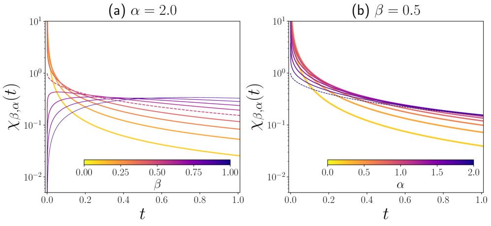
Figure 1: The waiting time density density $\chi_{\beta,\alpha}(t)$ as a function of $t$. We explore the results for (a) $\alpha=2.0$ for different values $0<\beta\leq 1$ and (b) $\beta=0.5$ for $0<\alpha\leq 2$ (in each case, the parameters are codified in the colorbar). Results were obtained numerically using $\xi=1$ and Eqs. (35) and (36). We depict with dashed lines the case when $\alpha\beta=1$.

The Prabhakar-Mittag-Leffler function (36) and related problems were analyzed by several authors [28, 29, 30, 31, 32].

In Figure 1(a) is drawn the waiting time PDF of Eq. (35) for a fixed value of $\it\alpha=2$ and variable $\beta$ in the admissible range $\it 0<\beta\leq 1$. The waiting time PDF exhibits for $\it t$ small the power-law behavior $\it\chi_{\beta,\alpha}(t)\approx\frac{\xi^{\alpha}}{\Gamma(\alpha\beta)}t^{\alpha\beta-1}$ (corresponding to the zero order in the expansion (35)) with two distinct regimes: For $\it\alpha\beta<1$ the waiting time PDF becomes singular at $\it t=0$ corresponding to ‘immediate’ arrivals of the first event. For $\it\alpha\beta=1$ the jump density takes the constant value $\it\chi_{\alpha^{-1},\alpha}(t=0)=\xi^{\alpha}$ whereas for $\it\alpha\beta>0$ the waiting time density $\it\chi_{\beta,\alpha}(t=0)=0$ tends to zero as $\it t\rightarrow 0$ where the waiting times become longer the larger $\alpha\beta$.

In Figure 1(b) we depict the behavior of the waiting time PDF for fixed $\it\beta=0.5$ and $\it 0<\alpha\leq 2$ thus $\it\alpha\beta\leq 1$. It can be seen that the smaller $\it\alpha\beta$ the more narrowly the waiting time PDF is concentrated at small $\it t$-values close to $\it t=0$. This behavior can also be identified in view of Laplace transform (34) which takes in the limit $\it\alpha\rightarrow 0$ the value $\it\lim_{\alpha\rightarrow 0}{\tilde{\chi}}_{\beta,\alpha}(s)=1$ thus $\it\chi_{\beta,0+}(t)={\cal L}^{-1}(1)=\lim_{\alpha\rightarrow 0}\frac{\xi^{\alpha}}{\Gamma(\alpha\beta)}t^{\alpha\beta-1}=\delta(t)$ exhibits the shape of a Dirac $\it\delta$-distribution peak.

Now our goal is to determine the generalization of the fractional Poisson distribution (29) which is determined by Eq. (9) with (34), namely

$$\it\Phi^{(n)}_{\beta,\alpha}(t)={\cal L}^{-1}\left\{\frac{1}{s}\left({\tilde{\chi}}^{n}_{\beta,\alpha}(s)-{\tilde{\chi}}^{n+1}_{\beta,\alpha}(s)\right)\right\}={\cal L}^{-1}\left\{\frac{1}{s}\left({\tilde{\chi}}_{\beta,n\alpha}(s)-{\tilde{\chi}}_{\beta,(n+1)\alpha}(s)\right)\right\},\hskip 14.22636ptn=0,1,2,\ldots$$ (38)

where it is convenient to utilize $\it{\tilde{\chi}}^{n}_{\beta,\alpha}(s)={\tilde{\chi}}_{\beta,n\alpha}(s)=\frac{\xi^{n\alpha}}{(\xi+s^{\beta})^{n\alpha}}$, i.e. to replace $\alpha\rightarrow n\alpha$ in the expression (35). We then obtain for the probability for $\it n$ arrivals within $\it[0,t]$ the expression

$$\it\displaystyle\Phi^{(n)}_{\beta,\alpha}(t)=\xi^{n\alpha}t^{n\alpha\beta}\left(E^{n\alpha}_{\beta,(n\alpha\beta+1)}(-\xi t^{\beta})-\xi^{\alpha}t^{\alpha\beta}E^{(n+1)\alpha}_{\beta,((n+1)\alpha\beta+1)}(-\xi t^{\beta})\right).$$ (39)

We refer this distribution to as the ‘generalized fractional Poisson distribution (GFPD)’ [17, 18]. This distribution was also obtained by Cahoy and Polito [16]. For $\it\alpha=1$ and $\it 0<\beta<1$ the GFPP (39) recovers the fractional Poisson distribution (29) and for $\it\alpha=1$, $\it\beta=1$ the standard Poisson distribution (21), and finally for $\it\alpha>0$ and $\it\beta=1$ the Erlang distribution [17, 18].

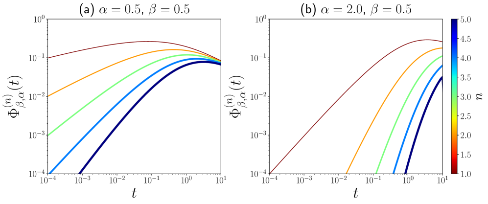
Figure 2: Probability $\Phi_{\beta,\alpha}^{(n)}(t)$ as a function of $t$ for different $n$. (a) $\alpha=0.5$ and $\beta=0.5$, (a) $\alpha=2.0$ and $\beta=0.5$. In the colorbar we represent $n=1,2,\ldots,5$. The values were obtained numerically using $\xi=1$ with Eq. (38). The results for $t\ll 1$ show the power-law relation $\Phi_{\beta,\alpha}^{(n)}(t)\propto t^{n\alpha\beta}$ in Eq. (40).

For applications in the dynamics in complex systems the asymptotic properties of the GFPD are of interest. For small (dimensionless) times the GFPD behaves as

$$\it\Phi^{(n)}_{\beta,\alpha}(t)\approx\frac{(\xi t^{\beta})^{n\alpha}}{\Gamma(n\alpha\beta+1)},\hskip 28.45274ptt\xi^{\frac{1}{\beta}}\rightarrow 0,\hskip 28.45274ptn=0,1,2,\ldots$$ (40)

representing the lowest non-vanishing order in (39). It follows that the GFPD fulfills the initial condition

$$\it\Phi^{(n)}_{\beta,\alpha}(t)\Big{|}_{t=0}=\delta_{n0},$$ (41)

reflecting that per construction at $\it t=0$ no event has arrived. Further of interest is the asymptotic behavior for large (dimensionless) times $\it t\xi^{\frac{1}{\beta}}$. To this end, let us expand the Laplace transform for small $\it s\rightarrow 0$ in (38) up to the lowest non-vanishing order in $\it\frac{s^{\beta}}{\xi}$ to arrive at

$$\it\Phi^{(n)}_{\beta,\alpha}(t)\approx\frac{\alpha}{\xi}{\cal L}^{-1}\{s^{\beta-1}\}=\frac{\alpha}{\Gamma(1-\beta)}\left(t\xi^{\frac{1}{\beta}}\right)^{-\beta},\hskip 14.22636ptt\xi^{\frac{1}{\beta}}\rightarrow\infty,\hskip 14.22636ptn=0,1,\dots,\infty$$ (42)

where this inverse power law holds universally for all $\it\alpha>0$ for $\it 0<\beta<1$ and is independent of the number of arrivals $\it n$ recovering the fractional Poisson distribution for $\it\alpha=1$ of Eq. (33). We notice that for large (dimensionless) observation times an universal $\it(t\xi^{\frac{1}{\beta}})^{-\beta}$ power-law decay occurs which is independent of the arrival number $\it n$ where $\it\alpha$ occurs only as a scaling parameter in relation (42). We interpret this behavior as quasi-ergodicity property, i.e. quasi-equal distribution of all ‘states’ $\it n$ for $t\xi^{\frac{1}{\beta}}$ large [17]. The fractional exponent $\it-\beta$ further is independent of $\it\alpha$ thus the power-law is of the same type as in the fractional Poisson process.

In the Figure 2(a) we have plotted the probabilities $\it\Phi^{(n)}_{\beta,\alpha}(t)$ of Eq. (39) for fixed $\it\alpha$ and $\it\beta$ for different arrival numbers $\it n$. One can see that for large times the $\it\Phi^{(n)}_{\beta,\alpha}(t)$ converge to the same universal behavior independent of $\it n$ which reflects the asymptotic power-law relation (42). On the other hand the asymptotic power-law behavior for small $t$ is shown in Figure 2(b) (See also relation (40)). The decay to zero $\it\lim_{t\rightarrow 0}\Phi^{(n)}_{\beta,\alpha}(t)\Big{|}_{t=0}\sim(\xi t^{\beta})^{n\alpha}\rightarrow 0$ ($\it n>0$) becomes the more pronounced the larger $\it n$. This behavior also can be interpreted that the higher $\it n$, the less likely are $\it n$ arrivals to happen within a small time interval of observation.

The GFPP and the fractional Poisson process for large observation times exhibit the same power-law asymptotic feature (See again asymptotic relation (42)). This behavior reflects the ‘asymptotic universality’ of the fractional Poisson dynamics, the latter was demonstrated in Ref. [33]. The inverse power-law decay occurring for $\it 0<\beta<1$ with fat-tailed waiting time PDF indeed is the source of non-Markovian behavior with long-time memory. In the entire admissible range $\it 0<\beta\leq 1$ the waiting time PDF $\it\chi_{\beta,\alpha}(t)$ and survival probability $\it\Phi^{(0)}_{\beta,\alpha}(t)$ maintain their good property of being completely monotonic functions, i.e. they fulfill

$$\it(-1)^{n}\frac{d^{n}}{dt^{n}}f(t)\geq 0,\hskip 28.45274ptn=0,1,2,\dots,\hskip 28.45274ptt>0.$$ (43)

An analysis of various aspects of completely monotonic functions is performed in our recent works [8, 34], and see the references therein.

5 CONTINUOUS-TIME RANDOM WALK ON NETWORKS

Having recalled above basic properties of renewal theory our goal is now to analyze stochastic motions on undirected networks and lattices that are governed by the GFPP renewal process. To develop our model we employ the continuous-time random walk (CTRW) approach by Montroll and Weiss [19] (and see also the references [2, 21, 22]). In the present section our aim is to develop a CTRW model for undirected networks in order to apply the theory to infinite $\it d$-dimensional integer lattices $\it\mathbb{Z}^{d}$.

We consider an undirected connected network with $\it N$ nodes which we denote with $\it p=1,\ldots,N$. The topology of the network is described by the positive-semidefinite $\it N\times N$ Laplacian matrix which is defined by [8, 12, 36, 37, 38, 39, 40]

$$\it L_{pq}=K_{p}\delta_{pq}-A_{pq}$$ (44)

where $\it{\mathbf{A}}=(A_{pq})$ denotes the adjacency matrix having elements $\it A_{pq}=1$ if a pair $\it pq$ of nodes is connected and $\it A_{pq}=0$ if a pair $\it pq$ is disconnected. Further we forbid that nodes are connected with themselves thus $\it A_{pp}=0$. In an undirected network adjacency and Laplacian matrices are symmetric. The diagonal elements $\it L_{pp}=K_{p}$ of the Laplacian matrix are referred to as the degrees of the nodes $\it p$ counting the number of neighbor nodes of a node $\it p$ with $\it K_{p}=\sum_{q=1}^{N}A_{pq}$. In order to relate the network topology with random walk features we introduce the one-step transition matrix $\it{\mathbf{W}}=(W_{pq})$ which is defined by [8, 12]

$$\it W_{pq}=\frac{1}{K_{p}}A_{pq}=\delta_{pq}-\frac{1}{K_{p}}L_{pq}.$$ (45)

Generally, the transition matrix is non-symmetric for networks with variable degrees $\it K_{i}\neq K_{j}$ $(i\neq j)$. The one-step transition matrix $\it W_{pq}$ defines the conditional probability that a random walker which is on node $\it p$ jumps in one step to node $\it q$ where in one step only neighbor nodes with equal probability $\it\frac{1}{K_{p}}$ can be reached. We see in definition (45) that the one-step transition matrix $\it\sum_{q=1}^{N}W_{pq}=1$ and $\it 0\leq W_{pq}\leq 1$ and also the $\it n$-step transition matrices $\it{\mathbf{W}}^{n}$ are (row-)stochastic [8].

Now let us assume that each step of the walker from one to another node is associated with a jump event or arrival in a CTRW with identical transition probability $\it(W_{pq})$ for a step from node $\it p$ to node $\it q$. We assume the random walker performs IID random steps at random times $\it 0\leq t_{1},t_{2},\ldots t_{n},\ldots,\infty$ in a renewal process with IID waiting times $\it\Delta t_{k}$ where the observation starts at $\it t=0$. To this end let us recall some basic relations holding generally, and then we specify the renewal process to be a GFPP.

Introducing the transition matrix $\it{\mathbf{P}}(t)=(P_{ij}(t))$ indicating the probability to find the walker at time $t$ on node $j$ under the condition that the walker at $\it t=0$ initially was sitting at node $\it i$, we can write [35, 41]

$$\it{\mathbf{P}}(t)={\mathbf{P}}(0)\sum_{n=0}^{\infty}\Phi^{(n)}(t){\mathbf{W}}^{n}$$ (46)

where we assume here a general initial condition $\it{\mathbf{P}}(t)|_{t=0}={\mathbf{P}}(0)$ which is fulfilled by accounting for the initial conditions $\it\Phi^{(n)}(t)_{t=0}=\delta_{n0}$. In this series the $\it\Phi^{(n)}(t)$ indicate the probabilities of $n$ (jump-) events in the renewal process, i.e. the probability that the walker performs $\it n$ steps within $\it[0,t]$ (See Eq. (5)), and $\it({\mathbf{W}}^{n})_{ij}$ indicates the probability that the walker in $\it n$ jumps moves from the initial node $\it i$ to node $\it j$. We observe in view of relation (13) together with $\it\sum_{j=1}^{N}({\mathbf{W}}^{n})_{ij}=1$ that the normalization condition $\it\sum_{j=1}^{N}P_{ij}(t)=\sum_{n=0}^{\infty}\Phi^{(n)}(t)=1$ is fulfilled. The convergence of series (46) can be easily proved by using that $\it{\mathbf{W}}$ has uniquely eigenvalues $\it|\lambda_{m}|\leq 1$ and with $\it|{\tilde{\chi}}(s)|\leq 1$ [8, 17]. Let us assume that at $\it t=0$ the walker is sitting on departure node $\it i$ thus the initial condition is given by $\it P_{ij}(0)=(\delta_{ij})$, then the Laplace transform of (46) writes [17]

$$\it{\tilde{\mathbf{P}}}(s)=\frac{\left(1-{\tilde{\chi}}(s)\right)}{s}\left\{{\mathbf{1}}-{\tilde{\chi}}(s){\mathbf{W}}\right\}^{-1}$$ (47)

where $\it{\tilde{\mathbf{P}}}(s)$ has the eigenvalues [17]

$$\it{\tilde{P}}(m,s)=\frac{\left(1-{\tilde{\chi}}(s)\right)}{s}\frac{1}{(1-\lambda_{m}{\tilde{\chi}}(s))},\hskip 28.45274ptm=1,\dots,N.$$ (48)

The $\it\lambda_{m}$ indicate the eigenvalues of the one-step transition matrix $\it{\mathbf{W}}$. This expression is the celebrated Montroll-Weiss formula [19] and occurs in various contexts of physics.

6 GENERALIZED SPACE-TIME FRACTIONAL DIFFUSION IN $\it\mathbb{Z}^{d}$

In this section our aim is to develop a CTRW which is a random walk subordinated to a GFPP. For the random walk on the network we allow long-range jumps which can be described when we replace the Laplacian matrix by its fractional power in the one-step transition matrix (45). In this way, the walker cannot only jump to connected neighbor nodes, but also to far distant nodes in the network [5, 6, 8, 34, 36, 37, 38, 39, 42, 43]. The model to be developed in this section involves both space- and time-fractional calculus. As an example we consider the infinite $\it d$-dimensional integer lattice $\it\mathbb{Z}^{d}$. The lattice points $\it\mathbf{p}=(p_{1},\ldots,p_{d})$ ($p_{j}\in\mathbb{Z}_{0}$) represent the nodes where we assume each node is connected to any of its $\it 2d$ neighbor nodes. The $\it\mathbb{Z}^{d}$ is an infinite cubic primitive $\it d$-dimensional lattice with lattice-constant one. In this network any node has identical degree $\it 2d$. The one-step transition matrix with the elements $\it W^{(\mu)}(\mathbf{p}-\mathbf{q})$ has then the canonic representation [8, 38]

$$\it W^{(\mu)}(\mathbf{p}-\mathbf{q})=\frac{1}{(2\pi)^{d}}\int_{-\pi}^{\pi}{\rm d}k_{1}\dots\int_{-\pi}^{\pi}{\rm d}k_{d}e^{i{\mathbf{k}}\cdot(\mathbf{p}-\mathbf{q})}\lambda^{(\mu)}(\mathbf{k})$$ (49)

with the eigenvalues

$$\it\lambda^{(\mu)}(\mathbf{k})=1-\frac{1}{{\cal K}^{(\mu)}}\eta^{\frac{\mu}{2}}(\mathbf{k}),\hskip 14.22636pt\eta({\mathbf{k}})=2d-2\sum_{j=1}^{d}\cos(k_{j}),\hskip 28.45274pt0<\mu\leq 2$$ (50)

where $\it{\mathbf{k}}=(k_{1},\ldots,k_{d})$ denotes the wave-vector with $\it-\pi\leq k_{j}\leq\pi$. One can show that the fractional index $\mu$ is restricted to the interval $\it 0<\mu\leq 2$ as a requirement for stochasticity of the one-step transition matrix [8, 34, 38]. In (50) the constant $\it{\cal K}^{(\mu)}$ can be conceived as a fractional generalization of the degree and is given by the trace of the fractional power of Laplacian matrix, namely [8, 34]

$$\it\it{\cal K}^{(\mu)}=\frac{1}{N}tr(\mathbf{L}^{\frac{\mu}{2}})=\frac{1}{N}\sum_{m=1}^{N}(\eta_{m})^{\frac{\mu}{2}}$$ (51)

where $\it\eta_{m}$ denote the eigenvalues of the Laplacian matrix (44) and in an infinite network the sum in (51) has to be performed in the limit $\it N\rightarrow\infty$. In the $\it\mathbb{Z}^{d}$ the fractional degree with Eq. (51) is then determined from [8, 34]

$$\it{\cal K}^{(\mu)}=\frac{1}{(2\pi)^{d}}\int_{-\pi}^{\pi}{\rm d}k_{1}\dots\int_{-\pi}^{\pi}{\rm d}k_{d}(\eta({\mathbf{k}}))^{\frac{\mu}{2}}$$ (52)

with the eigenvalues given in Eq. (50). It is necessary to account for the fractional degree since it plays the role of a normalization factor in the one-step transition matrix (See Eq. (45)).

For the present analysis it is sufficient to consider $\it{\cal K}^{(\mu)}$ as a (positive) constant where for $\it\mu=2$ recovers $\it{\cal K}^{(\mu=2)}=2d$ the degree of any node. The transition matrix (46) is then determined by its Laplace transform (47) which writes in the $\it\mathbb{Z}^{d}$ as

$$\it{\tilde{P}}^{(\mu)}(\mathbf{p-q},s)=\frac{\left(1-{\tilde{\chi}}(s)\right)}{s}\frac{1}{(2\pi)^{d}}\int_{-\pi}^{\pi}{\rm d}k_{1}\ldots\int_{-\pi}^{\pi}{\rm d}k_{d}{\tilde{P}}({\mathbf{k}},0)\frac{e^{i\mathbf{k}\cdot(\mathbf{p}-\mathbf{q})}}{(1-\lambda^{(\mu)}(\mathbf{k}){\tilde{\chi}}(s))}$$ (53)

where $\it{\tilde{P}}({\mathbf{k}},0)$ indicates the Fourier transform of the initial condition which has the Fourier representation

$$\it P^{(\mu)}(\mathbf{p}-\mathbf{q},t=0)=P_{0}(\mathbf{p}-\mathbf{q})=\frac{1}{(2\pi)^{d}}\int_{-\pi}^{\pi}{\rm d}k_{1}\dots\int_{-\pi}^{\pi}{\rm d}k_{d}e^{i{\mathbf{k}}\cdot(\mathbf{p}-\mathbf{q})}{\tilde{P}}({\mathbf{k}},0).$$ (54)

In order to analyze the diffusive limit of (53), i.e. its long-wave approximation it will be sufficient to account for the eigenvalues (50) for $\it k\rightarrow 0$ (where $\it k=|\mathbf{k}|$). Then we have with $\it\eta^{\frac{\mu}{2}}(\mathbf{k})\approx k^{\mu}$ the behavior

$$\it\lambda^{(\mu)}(\mathbf{k})\approx 1-\frac{1}{{\cal K}^{(\mu)}}k^{\mu},\hskip 28.45274pt0<\mu\leq 2,\hskip 14.22636ptk\rightarrow 0.$$ (55)

These equations hold so far for space-fractional walks for an arbitrary renewal process with waiting time PDF $\it\chi(t)={\cal L}^{-1}\{{\tilde{\chi}}(s)\}$.

Now let us consider a space-fractional walk subordinated to a GFPP with $\it{\tilde{\chi}}(s)={\tilde{\chi}}_{\beta,\alpha}(s)$ of Eq. (34). We denote the corresponding transition matrix of this stochastic motion as $\it{\mathbf{P}}^{(\mu)}_{\beta,\alpha}(t)$ which contains three index parameters $\it 0<\mu\leq 2$, $\it 0<\beta\leq 1$ and $\it\alpha>0$ and one time scale parameter $\it\xi$ (of units $\it sec^{-\beta}$). In order to derive the generalized space-time fractional diffusion equation it is convenient to proceed in the Fourier-Laplace domain. The Fourier-Laplace transform of the $\it{\mathbf{P}}^{(\mu)}_{\beta,\alpha}(t)$ is then with Eq. (53) given by the Montroll-Weiss equation

$${\tilde{P}}^{(\mu)}_{\beta,\alpha}(k,s) ={\tilde{P}}({\mathbf{k}},0)\frac{\left(1-{\tilde{\chi}}_{\beta,\alpha}(s)\right)}{s}\frac{1}{(1-{\tilde{\chi}}_{\beta,\alpha}(s)\lambda^{(\mu)}(\mathbf{k}))}={\tilde{P}}({\mathbf{k}},0)\frac{s^{-1}}{\left(1+\frac{{\tilde{\chi}}_{\beta,\alpha}(s)}{(1-{\tilde{\chi}}_{\beta,\alpha}(s))}\frac{\eta^{\frac{\mu}{2}}({\mathbf{k}})}{{\cal K}^{(\mu)}}\right)}$$ (56)

$$\approx{\tilde{P}}({\mathbf{k}},0)\frac{s^{-1}}{\left(1+\frac{{\tilde{\chi}}_{\beta,\alpha}(s)}{(1-{\tilde{\chi}}_{\beta,\alpha}(s))}\frac{k^{\mu}}{{\cal K}^{(\mu)}}\right)},\hskip 28.45274ptk\rightarrow 0$$ (57)

containing also the Fourier transform $\it{\tilde{P}}({\mathbf{k}},0)$ of the initial condition (54). The exact equation (56) can be rewritten as

$$\it-\frac{\xi^{\alpha}\eta^{\frac{\mu}{2}}({\mathbf{k}})}{{\cal K}^{(\mu)}}{\tilde{P}}^{(\mu)}_{\beta,\alpha}(k,s)=(s^{\beta}+\xi)^{\alpha}{\tilde{P}}^{(\mu)}_{\beta,\alpha}(k,s)-\xi^{\alpha}{\tilde{P}}^{(\mu)}_{\beta,\alpha}(k,s)+\frac{\xi^{\alpha}-(s^{\beta}+\xi)^{\alpha}}{s}{\tilde{P}}({\mathbf{k}},0),\hskip 14.22636ptk_{j}\in[-\pi,\pi].$$ (58)

Transforming back this equation into the causal time domain and by using Eqs. (54) and (53) yields the generalized time-fractional matrix equation

$$\it-\frac{\xi^{\alpha}}{{\cal K}^{(\mu)}}{\mathbf{L}}^{\frac{\mu}{2}}\cdot{\mathbf{P}}^{(\mu)}_{(\beta,\alpha)}(t)=_{0}\!\mathcal{D}_{t}^{\beta,\alpha}\cdot{\mathbf{P}}^{(\mu)}_{\beta,\alpha}(t)-\xi^{\alpha}{\mathbf{P}}^{(\mu)}_{\beta,\alpha}(t)+{\mathbf{P}}_{0}\left\{\xi^{\alpha}\Theta(t)-K^{(0)}_{\beta,\alpha}(t)\right\},\hskip 14.22636ptt\geq 0$$ (59)

which we refer to as ‘generalized space-time fractional Kolmogorov-Feller equation’ where $\it 0<\mu\leq 2$ with $\it 0<\beta\leq 1$ and $\it\alpha>0$. This equation was obtained and analyzed recently for normal walks ($\it\mu=2$) subordinated to a GFPP [17, 18]. Equations of the type (59) generally describe the generalized space-time fractional diffusion on undirected networks connecting the network topology (contained in Laplacian matrix $\mathbf{L}$) with the GFPP-governed stochastic motion on the network. We used notation $\it{\mathbf{L}}^{\frac{\mu}{2}}$ which denotes the fractional power of Laplacian matrix $\it{\mathbf{L}}$, and $\it{\mathbf{P}}^{(\mu)}_{(\beta,\alpha)}(t)$ the transition matrix with the initial condition $\it{\mathbf{P}}^{(\mu)}_{(\beta,\alpha)}(t=0)={\mathbf{P}}_{0}$ where all these matrices are defined in $\it\mathbb{Z}^{d}$. Since the $\it\mathbb{Z}^{d}$ is an infinite network, these are symmetric and circulant $\it\infty\times\infty$ matrices with elements $\it L^{(\mu)}(\mathbf{p}-\mathbf{q}),P^{(\mu)}_{(\beta,\alpha)}(\mathbf{p}-\mathbf{q},t),{\mathbf{P}}_{0}(\mathbf{p}-\mathbf{q})$, respectively, where $\it\mathbf{p},\mathbf{q}\in\mathbb{Z}^{d}$. In Eq. (59) we have introduced the causal convolution operator $\it{}_{0}\!\mathcal{D}_{t}^{\beta,\alpha}$ and the causal function $\it K^{(0)}_{\beta,\alpha}(t)$ which were obtained in explicit forms [17, 18]

$$\it\begin{array}[]{l}\it\displaystyle{\cal D}^{\beta,\alpha}(t)={\cal L}^{-1}\left\{(s^{\beta}+\xi)^{\alpha}\right\}=\frac{d^{\lceil\alpha\beta\rceil}}{dt^{\lceil\alpha\beta\rceil}}\left(\Theta(t)d^{\beta,\alpha}(t)\right)\\ \\ \displaystyle\hskip 14.22636pt=\frac{d^{\lceil\alpha\beta\rceil}}{dt^{\lceil\alpha\beta\rceil}}(\Theta(t)d^{\beta,\alpha}(t-\tau))=\left\{\begin{array}[]{l}\frac{d^{\lceil\alpha\beta\rceil}}{dt^{\lceil\alpha\beta\rceil}}\left(\Theta(t)t^{\lceil\alpha\beta\rceil-\beta\alpha-1}\sum_{m=0}^{\infty}\frac{\alpha!}{(\alpha-m)!m!}\frac{(\xi t^{\beta})^{m}}{\Gamma(\beta m+\lceil\alpha\beta\rceil-\beta\alpha)}\right),\hskip 14.22636pt\alpha\beta\notin\mathbb{N}\\ \\ \it\displaystyle\frac{d^{\alpha\beta}}{dt^{\alpha\beta}}\left(\delta(t)+\Theta(t)\frac{d}{dt}\sum_{m=0}^{\infty}\frac{\alpha!}{(\alpha-m)!m!}\frac{(\xi t^{\beta})^{m}}{\Gamma(m\beta+1)}\right),\hskip 28.45274pt\alpha\beta\in\mathbb{N}\end{array}\right.\\ \\ \it\displaystyle\hskip 14.22636pt=\left\{\begin{array}[]{l}\frac{d^{\lceil\alpha\beta\rceil}}{dt^{\lceil\alpha\beta\rceil}}\left(\Theta(t)t^{\lceil\alpha\beta\rceil-\beta\alpha-1}E_{\alpha,\beta,(\lceil\alpha\beta\rceil-\alpha\beta)}(\xi t^{\beta})\right),\hskip 28.45274pt\alpha\beta\notin\mathbb{N}\\ \\ \frac{d^{\alpha\beta}}{dt^{\alpha\beta}}\left(\delta(t)+\Theta(t)\frac{d}{dt}E_{\alpha,\beta,1}(\xi t^{\beta})\right),\hskip 28.45274pt\alpha\beta\in\mathbb{N}.\end{array}\right.\end{array}$$ (60)

In these expressions we introduced the ceiling function $\it\lceil\gamma\rceil$ indicating the smallest integer greater or equal to $\it\gamma$ and the function $E_{c,a,b}(z)=E^{-c}_{a,b}(-z)$ where $E^{u}_{v,w}(\zeta)$ indicating the Prabhakar-Mittag-Leffler function (36). The operator $\it{}_{0}\!\mathcal{D}_{t}^{\beta,\alpha}$ acts on a causal distribution $\it P(t)$ such as in Eq. (59) in the following way

$$\it_{0}\!\mathcal{D}_{t}^{\beta,\alpha}\cdot P(t)=\frac{d^{\lceil\alpha\beta\rceil}}{dt^{\lceil\alpha\beta\rceil}}\int_{0}^{t}d^{\beta,\alpha}(t-\tau)P(\tau){\rm d}\tau.$$ (61)

The function $\it K^{(0)}_{\beta,\alpha}(t)$ of equation (59) was obtained as

$$\it\it\displaystyle K^{(0)}_{\beta,\alpha}(t)={\cal L}^{-1}\left\{\frac{(s^{\beta}+\xi)^{\alpha}}{s}\right\}=\left\{\begin{array}[]{l}\Theta(t)t^{-\alpha\beta}E_{\alpha,\beta,1-\alpha\beta}(\xi t^{\beta}),\hskip 28.45274pt0<\alpha\beta<1\\ \\ \it\displaystyle\frac{d^{\lceil\alpha\beta\rceil-1}}{dt^{\lceil\alpha\beta\rceil-1}}\left(\Theta(t)t^{\lceil\alpha\beta\rceil-\beta\alpha-1}E_{\alpha,\beta,(\lceil\alpha\beta\rceil-\alpha\beta)}(\xi t^{\beta})\right)\hskip 14.22636pt\alpha\beta>1,\hskip 14.22636pt\alpha\beta\notin\mathbb{N}\\ \\ \it\displaystyle\frac{d^{\alpha\beta-1}}{dt^{\alpha\beta-1}}\left(\delta(t)+\Theta(t)\frac{d}{dt}E_{\alpha,\beta,1}(\xi t^{\beta})\right),\hskip 28.45274pt\alpha\beta\geq 1\in\mathbb{N}.\end{array}\right.$$ (62)

Equation (59) governs the ‘microscopic’ stochastic motions of the space fractional walk subordinated to a GFPP.

7 DIFFUSION-LIMIT

Our goal now is to determine the ‘diffusion-limit’ of above stochastic motion to obtain a ‘macroscopic picture’ on spatial scales large compared to the lattice constant $\it 1$ of the $\it\mathbb{Z}^{d}$. To this end it is sufficient to consider Montroll-Weiss equation (56) for $\it k$ small. Then Eq. (58) can be rewritten as

$$\it-\frac{\xi^{\alpha}k^{\mu}}{{\cal K}^{(\mu)}}{\tilde{P}}^{(\mu)}_{\beta,\alpha}({\mathbf{k}},s)\approx(s^{\beta}+\xi)^{\alpha}{\tilde{P}}^{(\mu)}_{\beta,\alpha}({\mathbf{k}},s)-\xi^{\alpha}{\tilde{P}}^{(\mu)}_{\beta,\alpha}({\mathbf{k}},s)+\frac{\xi^{\alpha}-(s^{\beta}+\xi)^{\alpha}}{s}{\tilde{P}}({\mathbf{k}},0),\hskip 14.22636ptk\rightarrow 0.$$ (63)

In order to derive the ‘diffusive limit’ which corresponds to the space-time representation of this equation, it appears instructive to consider the long-wave contribution of some kernels such as the fractional power of the Laplacian matrix in $\it\mathbb{Z}^{d}$. The fractional Laplacian matrix in $\it\mathbb{Z}^{d}$ has the canonic form [8, 38]

$$\it[{\mathbf{L}}^{\frac{\mu}{2}}]_{{\mathbf{p}}-\mathbf{q}}=\frac{1}{(2\pi)^{d}}\int_{-\pi}^{\pi}{\rm d}k_{1}\dots\int_{-\pi}^{\pi}{\rm d}k_{d}e^{i{\mathbf{k}}\cdot(\mathbf{p}-\mathbf{q})}\eta^{\frac{\mu}{2}}({\mathbf{k}}),\hskip 14.22636pt0<\mu\leq 2$$ (64)

where $\it\eta({\bf k})$ are the eigenvalues of the Laplacian matrix in $\it\mathbb{Z}^{d}$ defined by Eq. (50). Let us consider the contribution generated by small $\it k\rightarrow 0$ by integrating over a small $\it d$-cube $\it|k_{j}|\leq k_{c}\ll 1$ around the origin (corresponding to very large wave-lengths), namely

$$\it\begin{array}[]{l}\it\displaystyle[{\mathbf{L}^{\prime}}^{\frac{\mu}{2}}]_{{\mathbf{p}}-\mathbf{q}}\approx\frac{1}{(2\pi)^{d}}\int_{-k_{c}}^{k_{c}}{\rm d}k_{1}\dots\int_{-k_{c}}^{k_{c}}{\rm d}k_{d}e^{i{\mathbf{k}}\cdot(\mathbf{p}-\mathbf{q})}\eta^{\frac{\mu}{2}}({\mathbf{k}})\\ \\ \it\displaystyle=\frac{h^{d}}{(2\pi)^{d}}\int_{-\pi h^{-\frac{1}{2}}}^{\pi h^{-\frac{1}{2}}}{\rm d}{\bar{k}}_{1}\dots\int_{-\pi h^{-\frac{1}{2}}}^{\pi h^{-\frac{1}{2}}}{\rm d}{\bar{k}}_{d}e^{i{\bar{\mathbf{k}}}\cdot(\mathbf{p}-\mathbf{q})h}\eta^{\frac{\mu}{2}}(h{\bar{\mathbf{k}}}).\end{array}$$ (65)

In the second line we have introduced a new wave vector $\it{\bar{\mathbf{k}}}$ with $\it k_{j}={\bar{k}}_{j}h\leq k_{c}$ with $\it k_{c}(h)=\pi h^{\frac{1}{2}}\rightarrow 0$ small thus $\it 0\leq|{\bar{k}}_{j}|\leq\pi h^{-\frac{1}{2}}\rightarrow\infty$ (where any exponent $\it 0<\delta<1$ could be used with $\it|{\bar{k}}_{j}|\leq\pi h^{-\delta}\rightarrow\infty$ and $\it h{\bar{k}}_{j}\leq\pi h^{1-\delta}\rightarrow 0$). In this way the integral (65) (rescaled $\it h^{-d}$) over small $\it k$ becomes an integral over the complete infinite $\it{\bar{\mathbf{k}}}$-space where in this integration $\it k={\bar{k}}h$ is small. Hence $\it(\eta(h{\bar{k}}))^{\frac{\mu}{2}}\approx h^{\mu}{\bar{k}}^{\mu}\leq\pi^{\mu}h^{\frac{\mu}{2}}\ll 1$ remains valid in the entire region of integration in (65)₂. Introducing the rescaled quasi-continuous very slowly varying ‘macroscopic’ coordinates $\it(\mathbf{p}-\mathbf{q})h=\mathbf{r}-\mathbf{r}^{\prime}\in h\mathbb{Z}^{d}$ of the nodes we arrive at

$$\it[\mathbf{L^{\prime}}^{\frac{\mu}{2}}]_{{\mathbf{p}}-\mathbf{q}}\approx h^{\mu+d}\frac{1}{(2\pi)^{d}}\int_{-\infty}^{\infty}{\rm d}{\bar{k}}_{1}\dots\int_{-\infty}^{\infty}{\rm d}{\bar{k}}_{d}e^{i{\mathbf{\bar{k}}}\cdot(\mathbf{r}-\mathbf{r}^{\prime})}{\bar{k}}^{\mu}=h^{\mu+d}(-\Delta)^{\frac{\mu}{2}}\delta^{d}({\bf r}-{\bf r}^{\prime}).$$ (66)

The new macroscopic coordinates $\it{\mathbf{r}}=h{\mathbf{p}},\it{\mathbf{r}}^{\prime}=h{\mathbf{q}}\in\mathbb{R}^{d}$ are non-zero only for very large values of the integer values $\it p_{j}\sim h^{-1}\gg 1$, $\it q_{i}h^{-1}\gg 1$, i.e. the representation (66) captures the far-field contribution $\it|\mathbf{p}-\mathbf{q}|\gg 1$. In Eq. (66) $\it\Delta=\sum_{j=1}^{d}\frac{\partial^{2}}{\partial x_{j}^{2}}$ denotes the standard Laplacian with respect to the macroscopic coordinates $\it{\mathbf{r}}$. The Fourier integral coincides up to the sign with the kernel of the Riesz fractional derivative $\it-(-\Delta)^{\frac{\mu}{2}}\delta^{d}({\mathbf{r}}-{\mathbf{r}}^{\prime})$ of the $\it\mathbb{R}^{d}$ (which has the eigenvalues $\it-k^{-\mu}$ and also is referred to as fractional Laplacian recovering for $\it\mu=2$ the standard Laplacian $\it\Delta$) [8]. It follows that Eq. (63) can be transformed into the spatial (long-wave-) representation by

$$\it P^{(\mu)}(\mathbf{p}-\mathbf{q},t)\approx h^{d}{\bar{P}}^{(\mu)}(h(\mathbf{p}-\mathbf{q}),t),\hskip 28.45274pth\rightarrow 0$$ (67)

where we denote $\it h(\mathbf{p}-\mathbf{q})={\mathbf{r}}-{\mathbf{r}}^{\prime}\in\mathbb{Z}^{d}h\rightarrow\mathbb{R}^{d}$. The smooth field $\it{\bar{P}}^{(\mu)}({\bf r}-{\bf r}^{\prime},t)$ introduced in asymptotic relation (67) indicates the macroscopic transition probability density kernel having physical units $\it cm^{-d}$. By using Eqs. (53)-(56) and $\it\lambda^{(\mu)}(h{\bar{k}})\approx 1-\frac{h^{\mu}{\bar{k}}^{\mu}}{{\cal K}^{(\mu)}}$ we arrive at

$$\it{\bar{P}}^{(\mu)}({\mathbf{r}}-{\mathbf{r}}^{\prime},t)\approx{\cal L}^{-1}\left\{\frac{s^{-1}}{(2\pi)^{d}}\int_{-\infty}^{\infty}{\rm d}k_{1}\ldots\int_{-\infty}^{\infty}{\rm d}k_{d}e^{i{\mathbf{\bar{k}}}\cdot(\mathbf{r}-\mathbf{r}^{\prime})}\frac{{\bar{P}}(h{\bar{k}},0)}{\left(1+\frac{{\tilde{\chi}}_{\beta,\alpha}(s)}{1-{\tilde{\chi}}_{\beta,\alpha}(s)}\frac{h^{\mu}{\bar{k}}^{\mu}}{{\cal K}^{(\mu)}}\right)}\right\}$$ (68)

where the integration limits here can be thought to be generated by a limiting process $\it\pm\lim_{h\rightarrow 0}\pi h^{-\frac{1}{2}}\rightarrow\pm\infty$ in the same way as in integral (65) thus only small $\it h{\bar{k}}\leq\pi h^{\frac{1}{2}}$ in the integrand of (68) are relevant. Then let us rewrite Eq. (63) in the Fourier-Laplace domain in the form

$$\it-\frac{h^{\mu}{\bar{k}}^{\mu}}{{\cal K}^{(\mu)}}{\tilde{P}}^{(\mu)}_{\beta,\alpha}(h{\bar{k}},s)\approx\left[\left(1+\frac{s^{\beta}}{\xi}\right)^{\alpha}-1\right]{\tilde{P}}^{(\mu)}_{\beta,\alpha}(h{\bar{k}},s)+\frac{{\tilde{P}}(h{\bar{k}},0)}{s}\left[1-\left(1+\frac{s^{\beta}}{\xi}\right)^{\alpha}\right],\hskip 14.22636pth\rightarrow 0.$$ (69)

We observe that $\it h\rightarrow 0$ makes left-hand side converging to zero (as within the integration limits of integral (65) $\it k^{\mu}=h^{\mu}{\bar{k}}^{\mu}\leq\pi^{\mu}h^{\mu/2}\rightarrow 0$, i.e. only small $\it k=h{\bar{k}}$ are captured). In order to maintain the equality requires on the right-hand side of Eq. (69) $\it\xi\rightarrow\infty$ thus we can expand $\it(1+\frac{s^{\beta}}{\xi})^{\alpha}\approx 1+\frac{\alpha}{\xi}s^{\beta}$ and obtain

$$\it-\frac{\xi h^{\mu}{\bar{k}}^{\mu}}{\alpha{\cal K}^{(\mu)}}{\tilde{P}}^{(\mu)}_{\beta,\alpha}(h{\bar{k}},s)\approx s^{\beta}{\tilde{P}}^{(\mu)}_{\beta,\alpha}(h{\bar{k}},s)-{\tilde{P}}(h{\bar{k}},0)s^{\beta-1}.$$ (70)

The existence of the diffusive limit requires the left-hand side of this equation to remain finite, i.e. $\it\xi h^{\mu}=const$ when $\it h\rightarrow 0$. It follows that $\it\xi$ then scales as $\it\xi\sim h^{-\mu}$ leading to the new generalized diffusion constant

$$\it{\cal A}=\frac{\xi h^{\mu}}{\alpha{\cal K}^{(\mu)}}>0,\hskip 28.45274pt\alpha>0,\hskip 14.22636pt0<\mu\leq 2,$$ (71)

having physical dimension $\it cm^{\mu}sec^{-\beta}$. We obtain hence the universal diffusion-limit in the form of a space-time fractional diffusion equation of the form

$$\it-{\cal A}\left(-\Delta\right)^{\frac{\mu}{2}}\cdot{\bar{P}}^{(\mu)}_{(\beta,\alpha)}(r,t)=_{0}\!D_{t}^{\beta}\cdot{\bar{P}}^{(\mu)}_{\beta,\alpha}({\bf r},t)-{\bar{P}}_{0}({\bf r})\,\frac{t^{-\beta}}{\Gamma(1-\beta)}\hskip 28.45274pt0<\beta<1.$$ (72)

In this equation $\it{}_{0}D_{t}^{\beta}\cdot(\dots)$ denotes the Riemann-Liouville fractional derivative of order $\beta$ (See Appendix A.1, Eq. (104)), and $\it-\left(-\Delta\right)^{\frac{\mu}{2}}$ indicates the Riesz-fractional derivative convolution operator (fractional Laplacian) in the $d$-dimensional infinite space. The diffusion limit Eq. (72) is coinciding with a space-time fractional diffusion equation given by several authors [3, 6] in various contexts (among others). This equation is of the same type as the equation that occurs in the purely fractional Poisson process, i.e. for $\it\alpha=1$. We notice in view of the diffusion constant (71) that index $\it\alpha$ appears in Eq. (72) only as a scaling parameter. The universal space-time fractional behavior of the diffusive limit reflects the asymptotic universality of the Mittag-Leffler waiting time PDF which was demonstrated by Gorenflo and Mainardi [33]. We emphasize the non-Markovian characteristics of this time fractional diffusion process in the range $\it 0<\beta<1$, i.e. when the waiting time PDF is fat-tailed. The non-markovianity is reflected by the occurrence of the slowly decaying memory term $\it-{\bar{P}}_{0}({\bf r})\,\frac{t^{-\beta}}{\Gamma(1-\beta)}$ in Eq. (72) exhibiting a long-time memory of the initial condition $\it{\bar{P}}^{\mu}_{\beta,\alpha}({\bf r},t=0)={\bar{P}}_{0}({\bf r})$.

Let us briefly consider the case when the walker at $t=0$ is in the origin. The initial condition then is given by $\it{\bar{P}}_{0}({\bf r})=\delta^{d}({\bf r})$ and from Eqs. (70)-(72) follows that

$$\it{\tilde{P}}^{(\mu)}_{\beta,\alpha}(h{\bar{k}},s)=\frac{s^{\beta-1}}{{\cal A}{\bar{k}}^{\mu}+s^{\beta}}.$$ (73)

In view of Eq. (27) we obtain for the causal Fourier-time domain the solution

$$\it{\hat{P}}^{(\mu)}_{\beta,\alpha}(h{\bar{k}},t)={\cal L}^{-1}\left\{\frac{s^{\beta-1}}{{\cal A}{\bar{k}}^{\mu}+s^{\beta}}\right\}=\Theta(t)E_{\beta}(-{\cal A}{\bar{k}}^{\mu}t^{\beta}),\hskip 14.22636pt0<\beta\leq 1$$ (74)

where $\it E_{\beta}(z)$ denotes the Mittag-Leffler function defined in Eq. (100) and for later convenience we included the Heaviside-step function $\it\Theta(t)$. In the space-time domain the transition probability kernel is given by the Fourier inversion

$$\it{\bar{P}}^{(\mu)}_{\beta,\alpha}({\mathbf{r}},t)=\frac{\Theta(t)}{(2\pi)^{d}}\int_{-\infty}^{\infty}{\bar{d}}k_{1}\dots\int_{-\infty}^{\infty}{\bar{d}}k_{d}e^{i{\bar{\mathbf{k}}}\cdot{\mathbf{r}}}E_{\beta}(-{\cal A}{\bar{k}}^{\mu}t^{\beta})$$ (75)

where by accounting for $\it E_{\beta}(0)=1$ the initial condition $\it{\bar{P}}^{(\mu)}_{\beta,\alpha}({\mathbf{r}},0)=\delta^{d}({\mathbf{r}})$ is directly confirmed. For $\it 0<\beta<1$ the Mittag-Leffler function exhibits for $\it{\cal A}{\bar{k}}^{\mu}t^{\beta}\gg 1$ inverse power-law behavior, namely

$$\it{\hat{P}}^{(\mu)}_{\beta,\alpha}(h{\bar{k}},t)\approx{\cal L}^{-1}\left\{{\cal A}^{-1}{\bar{k}}^{-\mu}s^{\beta-1}\right\}={\cal A}^{-1}{\bar{k}}^{-\mu}\,\frac{t^{-\beta}}{\Gamma(1-\beta)}.$$ (76)

In the limit $\it\beta\rightarrow 1-0$ Eq. (72) with $\it P_{0}({\bf r})=\delta^{d}({\mathbf{r}})$ takes for $\it 0<\mu<2$ the form of a standard space-fractional Lévy flight diffusion equation

$$\it-{\cal A}\left(-\Delta\right)^{\frac{\mu}{2}}{\bar{P}}^{(\mu)}_{(1,\alpha)}(r,t)=\frac{\partial}{\partial t}{\bar{P}}^{(\mu)}_{(1,\alpha)}(r,t)-\delta^{d}({\mathbf{r}})\delta(t)$$ (77)

where $\it 0<\mu\leq 2$ is admissible. This walk is Markovian and hence memoryless due to the immediate vanishing of the memory term $\it-\delta^{(d)}({\mathbf{r}})\delta(t)$ for $\it t>0$. For $\it\mu=2$ this equation recovers Fick’s second law of normal diffusion. For $\it\beta=1$ the Mittag-Leffler function in (74) turns into the form of exponential $\it E_{1}(-{\cal A}{\bar{k}}^{\mu}t)=e^{-{\cal A}{\bar{k}}^{\mu}t}$ thus the Fourier integral (75) becomes

$$\it{\bar{P}}^{(\mu)}_{(1,\alpha)}(r,t)=\frac{\Theta(t)}{(2\pi)^{d}}\int_{-\infty}^{\infty}{\bar{d}}k_{1}\dots\int_{-\infty}^{\infty}{\bar{d}}k_{d}e^{i{\bar{\mathbf{k}}}\cdot{\mathbf{r}}}e^{-{\cal A}{\bar{k}}^{\mu}t},\hskip 14.22636pt0<\mu\leq 2.$$ (78)

One directly confirms that (78) solves (77) and is indeed the well-known expression for a symmetric Lévy distribution in $\mathbb{R}^{d}$ [5, 6, 8] (and many others). Further mention worthy is the case $\it\beta=1$ and $\it\mu=2$ for which Eq. (77) recovers the form of a normal diffusion equation (Fick’s second law) where (78) turns into the Gaussian distribution

$$\it {\bar{P}}^{(2)}_{(1,\alpha)}(r,t)=\Theta(t)\frac{e^{-\frac{r^{2}}{4{\cal A}t}}}{(4\pi{\cal A}t)^{\frac{d}{2}}}$$ (79)

which indeed is the well-known causal solution of Fick’s second law in $\it\mathbb{R}^{d}$.

8 CONCLUSIONS

We developed a Montroll-Weiss CTRW model for space-fractional walks subordinated to a generalization of Laskin’s fractional Poisson process, i.e. the fractional (long-range) jumps are performed with waiting time PDF according to a ‘generalized fractional Poisson process’ (GFPP). We obtained a space-time fractional diffusion equation by defining a ‘well-scaled’ diffusion limit in the infinite $\it d$-dimensional integer lattice $\it\mathbb{Z}^{d}$ with a combined rescaling of space- and time-scales. The index $\it\alpha>0$ of the GFPP appears in this space-time fractional diffusion equation only as a scaling parameter. This diffusion equation is of the same type as for $\it\alpha=1$ when the GFPP coincides with the pure Laskin’s fractional Poisson process and exhibits for $\it 0<\beta<1$ non-Markovian features (long-time memory), and for $\it\beta=1$ becomes a Markovian memoryless (Lévy-flight) diffusion equation of standard Poisson.

The GFPP contains three parameters, two index parameters $\it 0<\beta\leq 1$ and $\it\alpha>1$ and parameter $\it\xi$ defining a time scale. In the admissible range $\it 0<\beta\leq 1$, the waiting time PDF and the survival probability maintain their good properties of complete monotony. For $\it\alpha=1$ and $\it 0<\beta<1$ the equations of Laskin’s fractional Poisson process and for $\it\alpha=1$, $\it\beta=1$ the classical equations of the standard Poisson process are recovered, respectively. Some of the discussed results were obtained in recent papers [17, 18]. Generalizations of fractional diffusion as analyzed in the present paper are interesting models for a better understanding of the stochastic dynamics in complex systems. Since these models offer more parameters they are susceptible to be adopted to describe real-world situations.

Appendix A APPENDIX

A.1 LAPLACE TRANSFORMS AND FRACTIONAL OPERATORS

Here we derive briefly some basic mathematical apparatus used in the paper in the context of causal functions and distributions involving fractional operators and Heaviside-calculus. All functions and distributions considered are to be conceived as generalized functions and distributions in the Gelfand-Shilov sense [23]. Let us first introduce the Heaviside step-function

$$\it\Theta(t)=\left\{\begin{array}[]{l}1,\hskip 28.45274ptt\geq 0\\ \\ 0,\hskip 28.45274ptt<0.\end{array}\right.$$ (80)

A function is causal if it has the form $\it\Theta(t)f(t)$, i.e. is null for $\it t<0$ and non-vanishing only for non-negative times $\it t$. We introduce the Laplace transform of $\it\Theta(t)f(t)$ by

$$\it{\tilde{f}}(s)={\cal L}(f(t))=\int_{-\infty}^{\infty}e^{-st}\Theta(t)f(t){\rm d}t=\int_{0}^{\infty}f(t)e^{-st}{\rm d}t,\hskip 28.45274pts=\sigma+i\omega$$ (81)

with suitably chosen $\it\sigma>\sigma_{0}$ in order to guarantee convergence of (81). In view of the fact that (81) can be read as Fourier transform of the causal function $e^{-\sigma t}f(t)\Theta(t)$ it is straightforward to see that the Laplace inversion corresponds to the representation of this function as Fourier integral namely

$$\it e^{-\sigma t}f(t)\Theta(t)=\frac{1}{2\pi}\int_{-\infty}^{\infty}e^{i\omega t}{\tilde{f}}(\sigma+i\omega){\rm d}\omega$$ (82)

which can be rewritten as

$$\it f(t)\Theta(t)=\frac{e^{\sigma t}}{2\pi}\int_{-\infty}^{\infty}e^{i\omega t}{\tilde{f}}(\sigma+i\omega){\rm d}\omega=\frac{1}{2\pi i}\int_{-i\infty}^{+i\infty}e^{st}{\tilde{f}}(s){\rm d}s.$$ (83)

Sometimes when there is no time derivative involved we skip the Heaviside $\it\Theta(t)$-function implying that all expressions are written for $t\geq 0$. Then we mention that

$$\it\Theta(t)f(t)=\int_{-\infty}^{\infty}\delta(t-\tau)\Theta(\tau)f(\tau){\rm d}\tau$$ (84)

and introduce the shift operator $\it e^{-\tau\frac{d}{dt}}$ acting on a function $\it g(t)$ as $\it e^{-\tau\frac{d}{dt}}g(t)=g(t-\tau)$ thus

$$\it e^{-\tau\frac{d}{dt}}\delta(t)=\delta(t-\tau).$$ (85)

Substituting this relation into (84) yields

$$\it\Theta(t)f(t)=\left\{\int_{-\infty}^{\infty}e^{-\tau\frac{d}{dt}}\Theta(\tau)f(\tau){\rm d}\tau\right\}\,\,\delta(t)={\cal L}^{-1}\{{\tilde{f}}(s)\}={\tilde{f}}\left(\frac{d}{dt}\right)\,\,\delta(t)$$ (86)

where the operator $\it{\tilde{f}}(\frac{d}{dt})$ is related with the Laplace transform (81) by replacing $\it s\rightarrow\frac{d}{dt}$. Eq. (86) is the operator representation of the causal function $\Theta(t)f(t)$. A convolution of two causal functions $\it\Theta(t)f(t),g(t)\Theta(t)$ then can be represented by

$$\it\begin{array}[]{l}\displaystyle\int_{0}^{t}g(t-\tau)f(\tau){\rm d}\tau=\int_{-\infty}^{\infty}\int_{-\infty}^{\infty}\delta(t-\tau_{1}-\tau_{2})g(\tau_{1})\Theta(\tau_{1})f(\tau_{2})\Theta(\tau_{2}){\rm d}\tau_{1}{\rm d}\tau_{2},\hskip 28.45274ptt>0\\ \\ \displaystyle\left(\int_{-\infty}^{\infty}e^{-\tau_{1}\frac{d}{dt}}\Theta(\tau_{1})f(\tau){\rm d}\tau_{1}\right)\left(\int_{-\infty}^{\infty}e^{-\tau_{2}\frac{d}{dt}}\Theta(\tau_{2})f(\tau){\rm d}\tau_{2}\right)\delta(t)\\ \\ \displaystyle={\cal L}^{-1}\{{\tilde{g}}(s){\tilde{f}}(s)\}={\tilde{f}}\left(\frac{d}{dt}\right){\tilde{g}}\left(\frac{d}{dt}\right)\,\,\delta(t)={\tilde{g}}\left(\frac{d}{dt}\right){\tilde{f}}\left(\frac{d}{dt}\right)\,\ \delta(t)\end{array}$$ (87)

where it has been used $\it\delta(t-\tau_{1}-\tau_{2})=e^{-(\tau_{1}+\tau_{2})\frac{d}{dt}}\delta(t)$. We observe that in (86) and (87) the Laplace variable is replaced $\it s\rightarrow\frac{d}{dt}$ in the causal time domain. By considering $\it{\bar{f}}(t)\Theta(t)=f(t)\Theta(t)e^{-\lambda t}$ we observe that

$$\it f(t)\Theta(t)e^{-\lambda t}=\left\{\int_{-\infty}^{\infty}e^{-\tau(\lambda+\frac{d}{dt})}f(\tau)\Theta(\tau){\rm d}\tau\right\}\delta(t)={\tilde{f}}\left(\lambda+\frac{d}{dt}\right)\delta(t)$$ (88)

where $\it{\tilde{f}}(s)={\cal L}\{f(t)\}$. We are especially dealing with normalized (probability-) distributions

$$\it{\tilde{f}}(s=0)=1=\int_{-\infty}^{\infty}\Theta(t)f(t){\rm d}t.$$ (89)

A very important consequence of relations (86) and (87) is that they can be used to solve differential equations and to determine causal Green’s functions. As a simple example consider the trivial algebraic equation in the Laplace domain

$$\it(s+\xi)\,\,\frac{\xi}{(s+\xi)}=\xi,\hskip 28.45274pt\xi>0$$ (90)

takes with $\it{\cal L}^{-1}\left\{s+\xi\right\}=\frac{d}{dt}+\xi$ and $\it{\cal L}^{-1}\left\{\frac{\xi}{s+\xi}\right\}=\Theta(t)\xi e^{-\xi t}$ where on the right-hand side is used that $\it{\cal L}^{-1}\{1\}=\delta(t)$. In the causal time domain (90) then gives the representation

$$\it\left(\frac{d}{dt}+\xi\right)\,\left(\xi\Theta(t)e^{-\xi t}\right)=\xi\delta(t),$$ (91)

result which is straightforwardly confirmed, i.e. the normalized causal Green’s function of $\it\frac{d}{dt}+\xi$ is directly obtained as $\it(\frac{d}{dt}+\xi)^{-1}\xi\delta(t)=\Theta(t)\xi e^{-\xi t}$ where it is important that the $\it\Theta(t)$-function is taken into account in the Laplace inversion.

A less trivial example is obtained when considering fractional powers of operators. For instance let us consider in the Laplace domain the equation

$$\it(s^{\beta}+\xi)\,\frac{\xi}{(s^{\beta}+\xi)}=\xi,\hskip 28.45274pt\xi>0,\hskip 28.45274pt0<\beta\leq 1$$ (92)

which writes in the time domain

$$\it\left\{\left(\frac{d}{dt}\right)^{\beta}+\xi\right\}\,\Theta(t)g_{\beta,\xi}(t)=\xi\delta(t)$$ (93)

where the fractional derivative $\left(\frac{d}{dt}\right)^{\beta}$ is determined subsequently. The causal Green’s function $\it\Theta(t)g_{\beta,\xi}(t)$ is obtained from the Laplace inversion

$$\it g_{\beta,\xi}(t)={\cal L}^{-1}\left\{\frac{\xi}{s^{\beta}+\xi}\right\}.$$ (94)

The inversion is performed directly when taking into account

$$\it\frac{\xi}{(s^{\beta}+\xi)}=s^{-\beta}\frac{\xi}{(1+\xi s^{-\beta})}=\xi\sum_{n=0}^{\infty}(-1)^{n}\xi^{n}s^{-\beta(n+1)},\hskip 28.45274pt\sigma=\Re\{s\}>\xi^{\frac{1}{\beta}}$$ (95)

where $\it\sigma=\Re\{s\}>\xi^{\frac{1}{\beta}}$ guarantees convergence of this geometric series $\it\forall\omega=\Im\{s\}$, i.e. for the entire interval of integration of the corresponding Laplace inversion integral (88). On the other hand we have

$$\it s^{-\mu}={\cal L}\left\{\Theta(t)\frac{t^{\mu-1}}{\Gamma(\mu)}\right\},\hskip 28.45274pt\mu>0,\hskip 28.45274pt\sigma>0,$$ (96)

where we use the notation $\it\Gamma(\xi+1)=\xi!$ for the Gamma-function. We then arrive at

$$\it\begin{array}[]{l}\it\displaystyle\Theta(t)g_{\beta,\xi}(t)={\cal L}^{-1}\left\{\frac{\xi}{\xi+s^{\beta}}\right\}\\ \\ \it\displaystyle\hskip 14.22636pt=\sum_{n=0}^{\infty}(-1)^{n}\xi^{n+1}{\cal L}^{-1}\left\{s^{-\beta(n+1)}\right\}=\Theta(t)\sum_{n=0}^{\infty}(-1)^{n}\xi^{n+1}\frac{t^{n\beta+\beta-1}}{\Gamma(n\beta+\beta)}\end{array}$$ (97)

with

$$\it g_{\beta,\xi}(t)=\xi t^{\beta-1}\sum_{n=0}^{\infty}\frac{(-\xi t^{\beta})^{n}}{\Gamma(n\beta+\beta)}=\xi t^{\beta-1}E_{\beta,\beta}(-\xi t^{\beta}).$$ (98)

Here we have introduced the generalized Mittag-Leffler function, e.g. [4, 30, 44]

$$\it E_{\beta,\gamma}(z)=\sum_{n=0}^{\infty}\frac{z^{n}}{\Gamma(\beta n+\gamma)},\hskip 28.45274pt\beta,\gamma>0,\hskip 14.22636ptz\in\mathbb{C}$$ (99)

It follows that $\it\xi$ is a dimensional constant having units $\it sec^{-\beta}$ so that (98) has physical dimension of $\it sec^{-1}$ of a density. The result (98) also is referred to as Mittag-Leffler density and represents the waiting time density of Eq. (26) of the fractional Poisson renewal process introduced by Laskin [14]. Generally Mittag-Leffler type functions play a major role in time fractional dynamics. We further often use the Mittag-Leffler function which is defined as, e.g. [4, 30, 44]

$$\it E_{\beta}(z)=\sum_{n=0}^{\infty}\frac{z^{n}}{\Gamma(\beta n+1)},\hskip 28.45274pt\beta>0,\hskip 14.22636ptz\in\mathbb{C}$$ (100)

where with (99) we have $\it E_{\beta}(z)=E_{\beta,1}(z)$. The Mittag-Leffler function has the important property that for $\it\beta=1$ it recovers the exponential $\it E_{1}(z)=e^{z}$.

Riemann-Liouville fractional integral and derivative

Now let us derive the kernel of the fractional power of time-derivative operator of Eq. (93) where we consider now exponents $\it\gamma>0$. This kernel is then obtained with above introduced methods in the following short way

$$\it\begin{array}[]{l}\it\displaystyle{\cal L}^{-1}\{s^{\gamma}\}={\cal L}^{-1}\{s^{\lceil\gamma\rceil}s^{\gamma-\lceil\gamma\rceil}\}=e^{\sigma t}\left(\sigma+\frac{d}{dt}\right)^{\lceil\gamma\rceil}\left(\sigma+\frac{d}{dt}\right)^{\gamma-\lceil\gamma\rceil}\delta(t),\hskip 28.45274pt\gamma>0,\gamma\notin\mathbb{N}\\ \\ \it\displaystyle\hskip 14.22636pt=e^{\sigma t}\left(\sigma+\frac{d}{dt}\right)^{\lceil\gamma\rceil}\int_{-\infty}^{\infty}\frac{{\rm d}\omega}{(2\pi)}e^{i\omega t}(\sigma+i\omega)^{\gamma-\lceil\gamma\rceil}\\ \\ \it\displaystyle\hskip 14.22636pt=e^{\sigma t}\left(\sigma+\frac{d}{dt}\right)^{\lceil\gamma\rceil}\left\{e^{-\sigma t}\Theta(t)\frac{t^{\lceil\gamma\rceil-\gamma-1}}{(\lceil\gamma\rceil-\gamma-1)!}\right\}=\frac{d^{\lceil\gamma\rceil}}{dt^{\lceil\gamma\rceil}}\left(\Theta(t)\frac{t^{\lceil\gamma\rceil-\gamma-1}}{\Gamma(\lceil\gamma\rceil-\gamma)}\right).\end{array}$$ (101)

Here we introduced the ceiling function $\it\lceil\gamma\rceil$ indicating the smallest integer greater or equal to $\it\gamma$. In this way the Fourier integral in the second line is integrable around $\it\omega=0$ $\it\forall\sigma\geq 0$ since $\it\gamma-\lceil\gamma\rceil>-1$. We then obtain for the Laplace inversion

$$\it{\cal L}^{-1}\{s^{-\gamma}\}=\Theta(t)\frac{t^{\gamma-1}}{\Gamma(\gamma)},\hskip 28.45274pt\gamma>0$$ (102)

as a fractional generalization of integration operator. This kernel indeed can be identified with the kernel of the Riemann-Liouville fractional integral operator of order $\it\gamma$ [45, 46, 47] which recovers for $\gamma\in\mathbb{N}$ the multiple integer order integrations.

On the other hand the kernel (101) with explicit representation in (101)₃ can be conceived as the ‘fractional derivative’ operator $\it(\frac{d}{dt})^{\gamma}$. The fractional derivative acts on causal functions $\it\Theta(t)f(t)$ as

$$\it\begin{array}[]{l}\it\displaystyle{\cal L}^{-1}\{s^{\gamma}\}\cdot f(t)\Theta(t)=:_{0}\!D_{t}^{\gamma}f(t)=\frac{d^{\lceil\gamma\rceil}}{dt^{\lceil\gamma\rceil}}\int_{-\infty}^{\infty}\left\{\Theta(t-\tau)\frac{(t-\tau)^{\lceil\gamma\rceil-\gamma-1}}{{\Gamma(\lceil\gamma\rceil-\gamma)}}\right\}f(\tau)\Theta(t){\rm d}\tau,\\ \\ \it{}_{0}\!D_{t}^{\gamma}f(t)=\frac{1}{{\Gamma(\lceil\gamma\rceil-\gamma)}}\frac{d^{\lceil\gamma\rceil}}{d\tau^{\lceil\gamma\rceil}}\int_{0}^{t}(t-\tau)^{\lceil\gamma\rceil-\gamma-1}f(\tau){\rm d}\tau.\end{array}\hskip 28.45274pt\gamma>0$$ (103)

We identify in the last line this operator with the Riemann-Liouville fractional derivative [45, 46, 47] which recovers for $\gamma\in\mathbb{N}$ integer-order standard derivatives. We emphasize that (101) requires causality, i.e. a distribution of the form $\it f(t)\Theta(t)$ thus the Laplace transform captures the entire non-zero contributions of the causal distribution. In the diffusion equation (72) the Riemann-Liouville fractional derivative is of order $\it 0<\beta<1$ with $\it\lceil\beta\rceil=1$. In this case (103) then yields has representation

$$\it{}_{0}\!D_{t}^{\beta}f(t)=\frac{1}{\Gamma(1-\beta)}\frac{d}{dt}\int_{0}^{t}(t-\tau)^{-\beta}f(\tau){\rm d}\tau,\hskip 28.45274pt0<\beta<1,\hskip 14.22636ptt>0.$$ (104)

References

- [1] G. M. Zaslavsky, Chaos, fractional kinetics, and anomalous transport, Phys. Rep 371 (6), 461-580 (2002).
- [2] M. Shlesinger, Origins and applications of the Montroll-Weiss continuous time random walk, Eur. Phys. J. B (2017) 90: 93.
- [3] A.I. Saichev, G.M. Zaslavsky, Fractional kinetic equations: solutions and applications. Chaos 7, pp. 753-764 (1997).
- [4] R. Gorenflo, E. A.A. Abdel Rehim, From Power Laws to Fractional Diffusion: The Direct Way, Vietnam Journ. Math. 32 (SI), 65-75, 2004.
- [5] R. Metzler, J. Klafter, The Random Walk’s Guide to Anomalous Diffusion : A Fractional Dynamics Approach, Phys. Rep 339, pp. 1-77 (2000).
- [6] R. Metzler, J. Klafter, The restaurant at the end of the random walk: recent developments in the description of anomalous transport by fractional dynamics, J. Phys. A: Math. Gen. 37 R161-R208 (2004).
- [7] E. Barkai, R. Metzler, and J. Klafter, From continuous time random walks to the fractional Fokker-Planck equation, Phys. Rev. E 61, No. 1 (2000).
- [8] T. Michelitsch, A.P. Riascos, B.A. Collet, A. Nowakowski, F. Nicolleau, Fractional Dynamics on Networks and Lattices, ISTE-Wiley March 2019, ISBN : 9781786301581.
- [9] N. Masuda, M.A. Porter, R. Lambiotte, Random walks and diffusion on networks, Physics Reports 716–717, 1–58 (2017).
- [10] A.P. Riascos, J. Wang-Michelitsch, T.M. Michelitsch, Aging in transport processes on networks with stochastic cumulative damage, Phys. Rev. E 100, 022312 (2019).
- [11] G. Polya, Über eine Aufgabe der Wahrscheinlichkeitsrechnung betreffend die Irrfahrt im Strassennetz, Mathematische Annalen 83 (1921), 149-160.
- [12] J.D. Noh, H. Rieger, Random walks on complex networks, Phys. Rev. Lett. Vol. 92, No. 11. (2004).
- [13] O.N. Repin and A.I. Saichev, Fractional Poisson law. Radiophysics and Quantum Electronics, 43:738-741 (2000).
- [14] N. Laskin, Fractional Poisson process, Commun Nonlinear Sci Numer Simul, Vol. 8(3-4), 201-213 (2003).
- [15] N. Laskin, Some applications of the fractional Poisson probability distribution, J. Math. Phys. 50, 113513 (2009).
- [16] D. O. Cahoy, F. Polito, Renewal processes based on generalized Mittag-Leffler waiting times, Commun Nonlinear Sci Numer Simul, Vol. 18 (3), 639-650, 2013.
- [17] T. Michelitsch, A.P. Riascos, Continuous time random walk and diffusion with generalized fractional Poisson process (Submitted), Preprint: arXiv:1907.03830 [cond-mat.stat-mech].
- [18] T.M. Michelitsch, A.P. Riascos, Generalized fractional Poisson process and related stochastic dynamics (Submitted), Preprint: arXiv:1906.09704 [cond-mat.stat-mech].
- [19] E. W. Montroll and G. H. Weiss, Random walks on lattices II., J. Math. Phys, Vol. 6, No. 2, 167-181 (1965).
- [20] F. Mainardi, R. Gorenflo, E. Scalas. A fractional generalization of the Poisson processes. Vietnam Journ. Math. 32, 53-64. (2004) MR2120631.
- [21] H. Scher, M. Lax, Stochastic Transport in a Disordered Solid. I. Theory, Phys. Rev. B 7, 4491 (1973).
- [22] R. Kutner, J. Masoliver, The continuous time random walk, still trendy: fifty-year history, state of art and outlook, Eur. Phys. J. B (2017) 90: 50.
- [23] Gelfand I. M., Shilov, G. E. (1968), Generalized Functions, Vols. I, II, III, Academic Press, New York, 1968, reprinted by the AMS (2016).
- [24] W. Feller, An Introduction to Probability Theory and its Applications. Vol. I (3rd ed.). New York: Wiley (1968).
- [25] L. Beghin, E. Orsingher. Fractional Poisson processes and related random motions. Electron. J. Probab., 14(61), 1790-1826 (2009).
- [26] R. Hilfer, L. Anton, Fractional master equation and fractal time random walks, Phys. Rev. E 51 R848–R851 (1995).
- [27] T.R. Prabhakar, A singular integral equation with a generalized Mittag-Leffler function in the kernel, Yokohama Math. J. 19 , pp. 7-15 (1971).
- [28] A. M. Mathai, Some properties of Mittag-Leffler functions and matrix variant analogues: A statistical perspective, Fract. Calc. Appl. Anal., Vol. 13, No. 2 (2010).
- [29] A.K. Shukla , J.C. Prajapati, On a generalization of Mittag-Leffler function and its properties, J. Math. Anal. Appl. 336, pp. 797-811 (2007).
- [30] H.J. Haubold, A.M. Mathhai, R.K. Saxena, Mittag-Leffler functions and their applications, J. Appl. Math., 2011(298628):51 (2011).
- [31] R. Gara, R. Garrappa, The Prabhakar or three parameter Mittag-Leffler function: Theory and application Communications in Nonlinear Sciences and Numerical Simulation 56, 314-329 (2018).
- [32] R. Garra, R. Gorenflo, F. Polito, Z. Tomovski, Hilfer–Prabhakar derivatives and some applications, Applied Mathematics and Computation 242, 576-589 (2014).
- [33] R. Gorenflo, F. Mainardi, The asymptotic universality of the Mittag-Leffler waiting time law in continuous time random walks, Invited lecture at the 373. WE-Heraeus-Seminar on Anomalous Transport: Experimental Results and Theoretical Challenges, Physikzentrum Bad-Honnef (Germany), 12-16 July 2006.
- [34] A.P. Riascos, T.M. Michelitsch, B.A. Collet, A.F. Nowakowski, F.C.G.A. Nicolleau, Random walks with long-range steps generated by functions of Laplacian matrices, J. Stat. Mech. . Stat. Mech. (2018) 043404 .
- [35] D.R. Cox, Renewal Theory, Second edition, Methuen. London (1967).
- [36] A.P. Riascos, J. L. Mateos, Fractional dynamics on networks: Emergence of anomalous diffusion and Lévy flights. Phys. Rev. E 90, 032809 (2014).
- [37] A.P. Riascos and J.L. Mateos, Fractional diffusion on circulant networks: emergence of a dynamical small world, J. Stat. Mech. P07015 (2015).
- [38] T.M. Michelitsch, B.A. Collet, A.P. Riascos, A.F. Nowakowski, F.C.G.A. Nicolleau, On recurrence of random walks with long-range steps generated by fractional Laplacian matrices on regular networks and simple cubic lattices. Journal of Physics A: Mathematical and Theoretical 50:505,004 (2017).
- [39] T. Michelitsch, B. Collet., A.P. Riascos, A. Nowakowski., F. Nicolleau, On Recurrence and Transience of Fractional Random Walks in Lattices, H. Altenbach, J Pouget, M. Rousseau, B. Collet, T. Michelitsch, Eds., Generalized Models and Non-classical Approaches in Complex Materials 1, p. 555–580, Springer International Publishing, Cham, 2018.
- [40] T.M. Michelitsch, B.A. Collet, A.F. Nowakowski, F.C.G.A. Nicolleau, Fractional Laplacian matrix on the finite periodic linear chain and its periodic Riesz fractional derivative continuum limit, J. Phys. A: Math. Theor. 48, 295202 (2015).
- [41] R. Gorenflo, Mittag-Leffler Waiting Time, Power Laws, Rarefaction, Continuous Time Random Walk, Diffusion Limit, arXiv:1004.4413 [math.PR] (2010).
- [42] A.P. Riascos, J.L. Mateos, Long-range navigation on complex networks using Lévy random walks, Phys. Rev. E 86 , 056110 (2012).
- [43] T.M. Michelitsch, B.A. Collet, A.P. Riascos, A.F. Nowakowski, F.C.G.A. Nicolleau, Fractional random walk lattice dynamics, . Phys. A: Math. Theor. 50 055003 (2017).
- [44] Gorenflo R., Kilbas A.A., Mainardi F., Rogosin S.V., Mittag-Leffler Functions, Related Topics and Applications (Springer, New York, 2014).
- [45] K.B. Oldham, J. Spanier, The fractional calculus (Academic Press, New York, 1974).
- [46] K.S. Miller, B. Ross, An Introduction to the Fractional Calculus and Fractional Differential Equations, (Wiley & Sons,New York, 1993).
- [47] S.G. Samko, A.A. Kilbas, O.I. Marichev, Fractional integrals and derivatives : theory and applications, Switzerland ; Philadelphia, Pa., USA : Gordon and Breach Science Publishers (1993).