Characterizing Deep Learning Training Workloads on Alibaba-PAI

Abstract

Modern deep learning models have been exploited in various domains, including computer vision (CV), natural language processing (NLP), search and recommendation. In practical AI clusters, workloads training these models are run using software frameworks such as TensorFlow, Caffe, PyTorch and CNTK. One critical issue for efficiently operating practical AI clouds, is to characterize the computing and data transfer demands of these workloads, and more importantly, the training performance given the underlying software framework and hardware configurations. In this paper, we characterize deep learning training workloads from Platform of Artificial Intelligence (PAI) in Alibaba. We establish an analytical framework to investigate detailed execution time breakdown of various workloads using different training architectures, to identify performance bottleneck. Results show that weight/gradient communication during training takes almost 62% of the total execution time among all our workloads on average. The computation part, involving both GPU computing and memory access, are not the biggest bottleneck based on collective behavior of the workloads. We further evaluate attainable performance of the workloads on various potential software/hardware mappings, and explore implications on software architecture selection and hardware configurations. We identify that 60% of PS/Worker workloads can be potentially sped up when ported to the AllReduce architecture exploiting the high-speed NVLink for GPU interconnect, and on average 1.7X speedup can be achieved when Ethernet bandwidth is upgraded from 25 Gbps to 100 Gbps.

I Introduction

Recent years have witnessed the proliferation of deep learning models used in various domains of the industry, including image processing [1, 2], video understanding [3, 4], language understanding [5, 6], speech recognition [7, 8], commodity search and recommendation [9, 10], autonomous drive [11], and various others [12, 13]. Large IT companies are investing substantially to build large AI clouds/clusters, equipped with expensive hardware such as GPUs, to run various deep learning workloads to support their AI-driven services.

This paper presents a characterization of the workloads from Platform of Artificial Intelligence (PAI) in Alibaba. PAI is a ML(machine learning)-as-a-service platform that simplifies machine learning adoption and makes large-scale AI to meet the needs of Alibaba internel business. It has also been shipped to Aliyun as a cloud product to serve public users. Thousands of training jobs are submitted to PAI on a daily basis, with different business objectives, and diversified computing, communication and I/O requirements and constraints. This paper focuses on one critical aspect of these practical workloads: characterize various resource requirements and identify performance bottlenecks given software frameworks and hardware configurations. The observations are intended to instruct exploration of the workload optimization space, and guide software and hardware configurations/provisioning, to improve workload execution performance.

Existing AI workload characterization work mostly focus on quantitative, precise performance modeling of AI workloads [14, 15] or building benchmark platforms to measure model performance [16, 17, 18] (see Sec. VII for detailed discussions). We take a different angle, collectively characterizing behavior of thousands of training jobs in a production cluster, as well as projecting potential performance gains with different software architectures and hardware configurations based on a simple analytical model. Contributions of this work are summarized as follows:

First, we present a lightweight framework to characterize the production workloads at the cluster level. We comprehensively include not only the basic aspects of computation and weight communication in training jobs, as considered in previous studies [19, 16], but also the input data I/O aspects. Our analysis shows that the data I/O time is non-negligible, especially for single-node training workloads; for distributed workloads, input data I/O can potentially become the performance bottleneck after gradient communication has been optimized.

Second, our statistical analysis of the cluster workloads reveals that multi-GPU interconnect rather than the computation power is more likely the bottleneck under the current widely adopted training architectures and system configurations. Previous work largely focus on analyzing computation resource and memory access of AI workloads [20, 16]. Shi et al. [21] study the communication factor, and make a similar conclusion that the current DL frameworks, including TensorFlow, CNTK and MXNet, do not perform well in scalability via Ethernet interconnect; their analysis is mainly focusing on performance comparison among different DL frameworks. Instead, we investigate the impact of data traffic on workload performance by collectively investigating a large number of training jobs, and explore potential optimization approaches for communication reduction.

Third, we establish simple analytical performance models based on the key workload features, aiming at exposing fundamental performance bottlenecks. Our analytical modeling is different from previous characterization methods [20, 22, 16], most of which adopt actual runtime profiling measurements for bottleneck analysis. Based on the analytical models, we estimate potential performance gains if the workloads were running on different software architectures and hardware configurations. The focus is to investigate which system architecture (PS/worker or AllReduce) should be adopted, how much benefits high-speed multi-GPU interconnect, NVLink, may bring, and how performance bottlenecks may shift with different architecture and hardware configurations.

Finally, we conduct detailed analysis of representative deep learning workloads using both analytical models and testbed experiments, in the domains of commodity embedding, search and recommendation, etc. The relevant models are becoming more and more important in companies related to e-commerce, social networking and search engines, and in PAI, consume a large fraction of resources. Results of the case studies show that differences between estimated performance using our analytical method and actual measurements are less than 10% on average. Based the basic workload features, we explore different optimization techniques upon different types of workloads, including mixed-precision training with TensorCore [23], operation fusion via XLA [24] and also changing the system architectures. We summarize useful observations and implications on improving practical deep learning training workloads.

II Background and Methodology

We first present our workload characterization framework. While the characterization framework is established based on TensorFlow [25], the methodology applies to other frameworks [26, 27, 28, 29] as well.

II-A Architecture Components Modeling

II-A1 System Infrastructure & Configuration

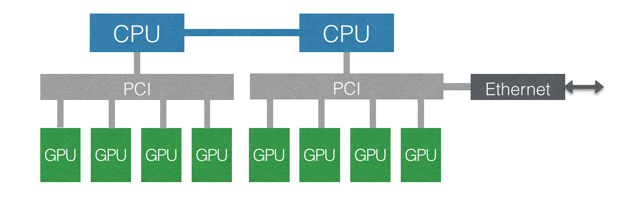
(a) Server without NVLink

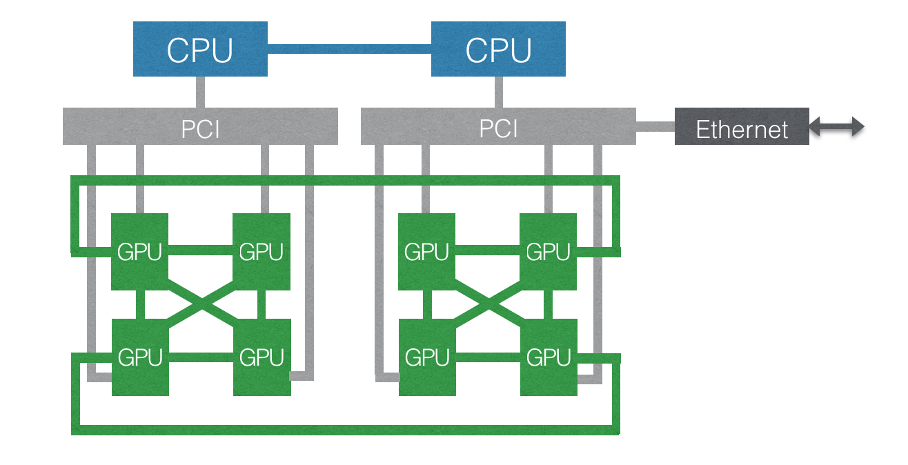
(b) Server with NVLink

Figure 1: System Infrastructure.

Figure 1 shows the basic server configurations in the AI cluster. There are typically two types of multi-GPU servers, equipped with/without NVLink [30]. The NVLink technology provides high-speed interconnect across multiple GPUs with a ‘hybrid mesh grid’ topology, as show in Fig. 1(b), to resolve the bandwidth bottleneck of PCIe interconnect among the GPUs. Due to cost issue, servers in some sub-clusters of PAI are equipped with NVLink, while others are not yet.

The basic server configuration where we collect the workload traces is shown in Table I. The servers are interconnected via bi-directional 25Gbps Ethernet. We will further discuss the impact of the system configurations through varying the configuration settings in Sec. III-C.

TABLE I: System Settings.

GPU	FLOPs	11 TFLOPs
	Memory	1 TB / second
Bandwidth	Ethernet	25 Gb / second
	PCI	10 GB / second
	NVLink	50 GB / second

II-A2 System Architecture

More than 85% computation resources on our cluster are used by distributed training workloads. DL training workloads can be parallelized via data parallelism, model parallelism and also hybrid parallelism [31]. While model parallelism and hybrid parallelism enable training neural networks which a single processor cannot support, they usually require significant human efforts for efficient model partition. Data parallelism is more model agnostic, and has been the most widely used paradigm for parallelizing neural network training [32]. We focus on data-parallel training jobs in this work.

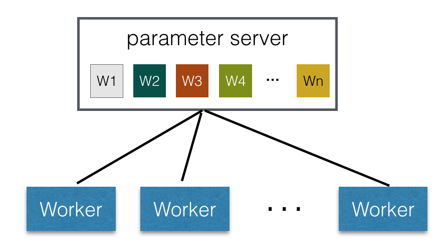
(a) PS/Worker

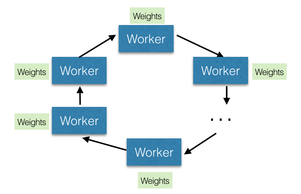
(b) AllReduce

Figure 2: System Architecture.

There are two types of system architectures, centralized and decentralized, for synchronizing weights/gradients among distributed training replicas. In a (parameter) centralized architecture, represented by the parameter server (PS) architecture [33], one or multiple parameter servers manage the gradient aggregation, and each worker holds a training replica, pulling variables from the PSs at the beginning in each training step and pushing gradients back to them at the end of each step. In a (parameter) decentralized architecture, the global parameters are placed replicated or partitioned on all training nodes; each training node exchanges the gradients via an AllReduce operation at the end of each training iteration. This architecture can benefit from the NVIDIA Collective Communications Library (NCCL) [34] for high-speed multi-node/multi-GPU communication. In this paper, we have implemented a new decentralized parallel training strategy called PEARL to handle large embedding weights. The detailed discussions about PEARL are showed in Sec. IV-C.

Currently, representative deep learning frameworks such as TensorFlow, Pytorch and MXNet mainly support the decentralized architecture in the replica mode: all model parameters are replicated to each device and data parallelism is used with the AllReduce algorithnm. In our cluster, roughly 29% jobs are running using the PS architecture and less than 1% using AllReduce, as we adopt AllReduce only after our cluster are equipped with NVLink.

II-A3 DL Training Workloads

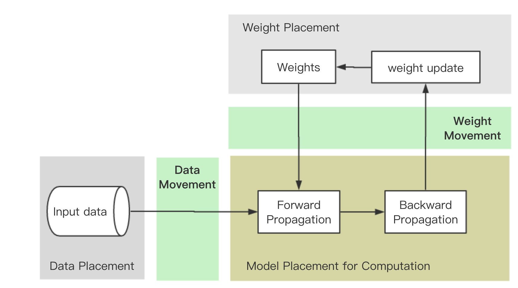
Figure 3: Data Flow of A Typical DL Training Step.

A DL training job always runs in an iterative fashion. Fig. 3 shows the basic workflow in a typical training step. We study impact of placement of the input data, model computation and weight update on runtime behavior of a training job. Weight movement refers to data transfer related to trainable parameters, including variable reading/gradient aggregation, respectively, in forward/backward stages. The data movement involves storage I/O, i.e., feeding training samples. For GPU workloads, the main computation is placed on GPUs while the data is in the CPU memory; therefore, input data I/O involves traffic on the CPU-GPU interconnect, i.e., PCIe.

Previous workload characterization work [16, 17] mainly focus on measuring the relationship between model computation and weight movement traffic, while ignoring the data part. However, we found that data I/O is a non-negligible factor for the runtime performance, especially for single-node training workloads.

We denote the non-distributed training workloads as 1w1g (single-worker-single-GPU), and classify our distributed training workloads into four types:

• 1wng: centralized training placed locally within a single server. Typically the parameters are placed on CPU while the computation model is replicated across multiple GPUs.

• PS/Worker: PS training framework with each worker/PS node being placed on a separate server.

• AllReduce-Local: AllReduce workloads in the local mode, running on individual servers equipped with NVLink to exploit the high-speed multi-GPU interconnect.

• AllReduce-Cluster: AllReduce workloads running across multiple servers.

TABLE II: Summary of five types of workloads in our cluster.

	System	System	Weight
	Architecture	Configuration	Movement
1w1g	-	Local	-
1wng	Centralized	Local	PCIe
PS/Worker	Centralized	Cluster	Ethernet & PCIe
AllReduce-Local	Decentralized	Local	NVLink
AllReduce-Cluster	Decentralized	Cluster	Ethernet & NVLink

Table II summarizes the basic features for each type of workloads. The common features among different types of workloads are not listed. For example, for all types model computation is placed on GPUs and the input data I/O is via PCIe from CPU to GPUs.

II-B Workload Characterization Framework

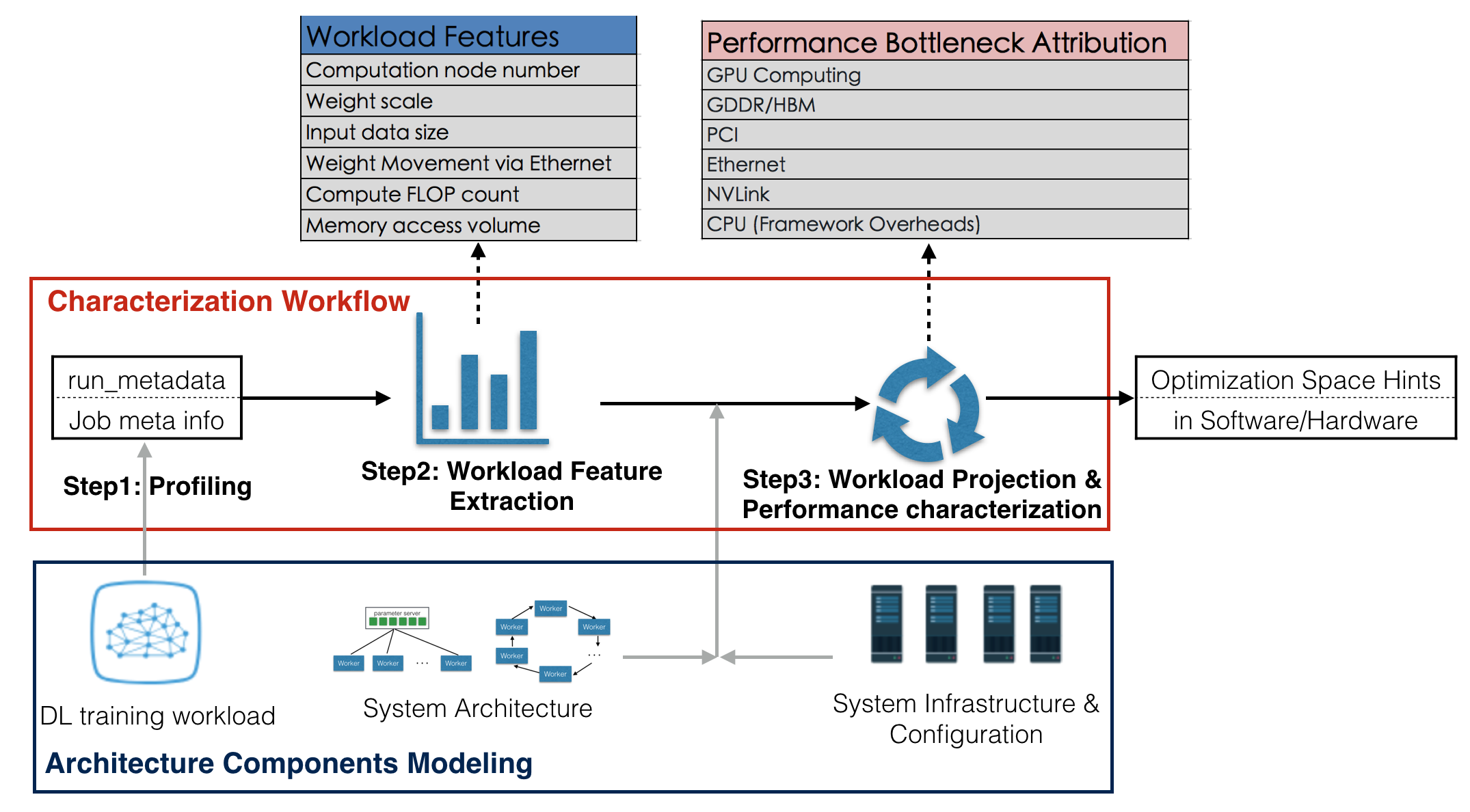
Figure 4: Workload Characterization Framework.

To analyze workload performance on our cluster, we established a workload characterization framework, as shown in Fig. 4.

II-B1 Runtime Profiling

TensorFlow provides a basic profiling tool, tf.RunMetadata() [35], which can trace the runtime information including device placement, operation attributes, kernel launch & execution time, and tensor attributes (data type, shape, allocation time and liveness, etc).

We further collect the job meta information, which mainly includes the resource allocation information in the entire job. For example, for a distributed training job in the PS/Worker architecture, run_metadata provides behavior of a single computation node (using one GPU device), and the job meta information provides supplementary information such as how many workers the job uses. Data collected through run_metadata and the job meta information constitute the raw data for our workload analysis.

II-B2 Workload Feature Extraction

We extract workload features from the fine-grained information collected, which characterize the execution requirements of each job in computation, I/O and weight/gradient transfer. Our workload feature schema is shown in Fig. 4.

II-B3 Performance Breakdown

For a given training job, we are interested in the composition of its execution time: input data I/O time ($T_{d}$), computation time ($T_{c}$) and weight/gradient communication time ($T_{w}$). In practice, sophisticated optimizations are possible to overlap computation and data transfer [36, 37]. Our goal is not to precisely model the total execution time, but to characterize the relative time consumption among computation, input I/O and weight/gradient communication. Therefore, potential overlap is not considered in our analysis and summation of all parts is used as the prediction of the total execution time for one training iteration/step: $T_{total}=T_{d}+T_{c}+T_{w}$.

Input data I/O time. $T_{d}$ measures the transport efficiency to load the input data, computed as $T_{d}=\frac{S_{d}}{B_{d}}$, where $S_{d}$ is the input data size and $B_{d}$ is the bandwidth for input data transfer.

Weight movement time. $T_{w}$ can be estimated using $T_{w}=\frac{S_{w}}{B_{w}}$, where $S_{w}$ denotes the weight size to be transferred across different model replicas within a training step, and $B_{w}$ is the bandwidth of the communication medium.

Computation time. The operations in DL workloads are divided into compute-bound and memory-bound ones. FLOP count, denoted as $\#FLOPs$, is adopted to measure the computation requirements by compute-bound operations (e.g., convolution and MatMul). The memory-bound operations, known as element-wise operations, spend more time on memory access, and thus the amount of memory access is used as their resource requirement. Let $S_{mem\_access}$ represent the total data size of memory access. The computation time can be computed as the sum of the two parts:

$$T_{c}=\frac{\#FLOPs}{peak\_FLOPs}+\frac{S_{mem\_access}}{B_{mem\_access}},$$ (1)

where $peak\_FLOPs$ and $B_{mem\_access}$ denote computation capacity and memory access bandwidth of the GPU, respectively. In practice, $peak\_FLOPs$ and $B_{mem\_access}$/$B_{d}$/$B_{w}$ are usually not fully used by a workload. Therefore, we use 70% of the actual capacities in the denominators when computing $T_{c}$/$T_{d}$/$T_{w}$ in our analysis. How to measure the utilization more precisely will be part of our future work.

The time percentage of each component is further computed by dividing the time of each component by the total time, e.g., percentage of the input data I/O time is $\frac{T_{d}}{T_{total}}$.

III Performance Characterization: Collective Behaviors

In this section, we conduct statistical analysis of tens of thousands of jobs running on PAI within the period of Dec. 1st, 2018 to Jan. 20th, 2019. The workloads are run on our internal TensoFlow framework, which is compatible with community TensorFlow 1.8. Due to the small amount of AllReduce jobs within this period, we focus on the analysis of 1w1g, 1wng and PS/Worker workloads from our cluster, and will further explore how much potential improvement can be achieved if using the AllReduce-based decentralized architecture.

III-A Overview of the Workloads

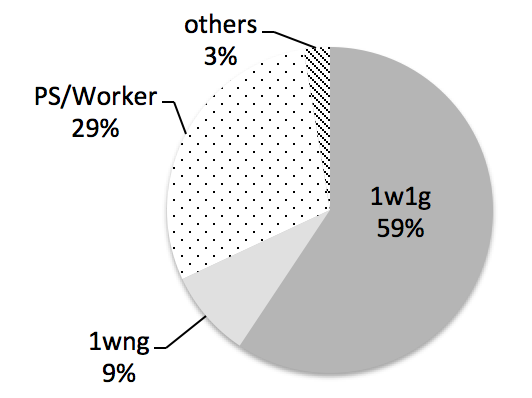
(a) job-level

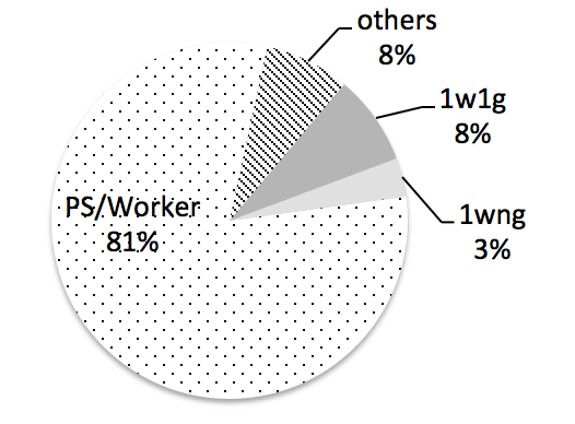
(b) cNode-level

Figure 5: Constitution of Workloads.

Composition of different types of workloads is shown in Fig. 5. Besides job numbers, we also count the numbers of computation nodes. A computation node, or cNode, is a GPU device holding a single computation model replica. At job-level, 1w1g dominates the job types; after taking the cNodes number in jobs into consideration, PS/Worker jobs consume the largest portion of resources, up to 81%.

(a) computation scale

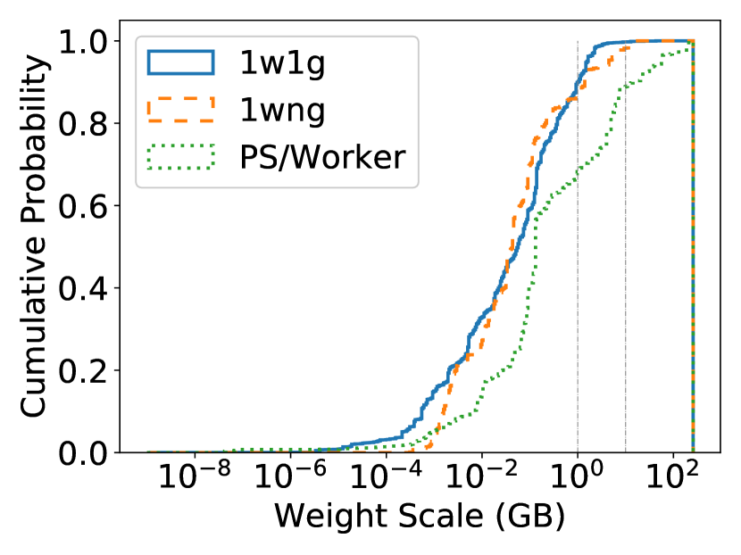
(b) weight size

Figure 6: Workload Scale Distribution.

We further show the cumulative distribution function (CDF) of the cNode number in each type of workloads in Fig. 6(a). For 1w1g workloads, the number of cNode is always 1; 1wng workloads are placed within a physical server typically, the number of cNodes is no more than 8; about half of PS/Worker workloads are placed on more than 8 cNodes, while a small fraction of jobs on more than 128 cNodes. This can help explain why there is only 29% workloads using the PS/Worker architecture, but the percentage of cNodes they consume is up to 81%.

The amount of computation resources consumed by a job can reflect the problem scale and may also indicate the commercial value of the workload. In our cluster, commodity embedding, search and recommendation workloads have large training datasets and may exploit hundreds to thousands of workers to achieve high throughput on the huge training dataset. Notably, such extra large-scale workloads always have significant commercial impact on the company’s business; however, they are often not included in DL workload benchmarks [16, 22]. We find that they are non-negligible: only 0.7% of all workloads have more than 128 cNodes; however, they consume more than 16% computation resource on our cluster. In the following Sec. IV, we will explore the characteristics of such large-scale workloads using two example jobs in detail.

The model size in a job is a key factor to decide what system architecture is best for the job. For example, for small to medium scale models that can fit into the GPU memory entirely, the AllReduce-Local configuration can be adopted, with better performance while using less system resources. When the weight size is large (ranging from tens to hundreds of GB), PS/Worker architecture should be adopted to partition the variables among multiple PS nodes (note that only weight-replica mode is supported in AllReduce implementation in representation DL frameworks). Fig. 6(b) illustrates the weight size distribution. We can observe that, within PS/Worker workloads, some jobs have large weight size, more than 10 GB or even 100 GB; however lots of them have quite small model sizes. So why do they choose to adopt the PS/Worker architecture? Can they be further optimized using a better model placement and system architecture? We will answer these questions in Sec. III-C.

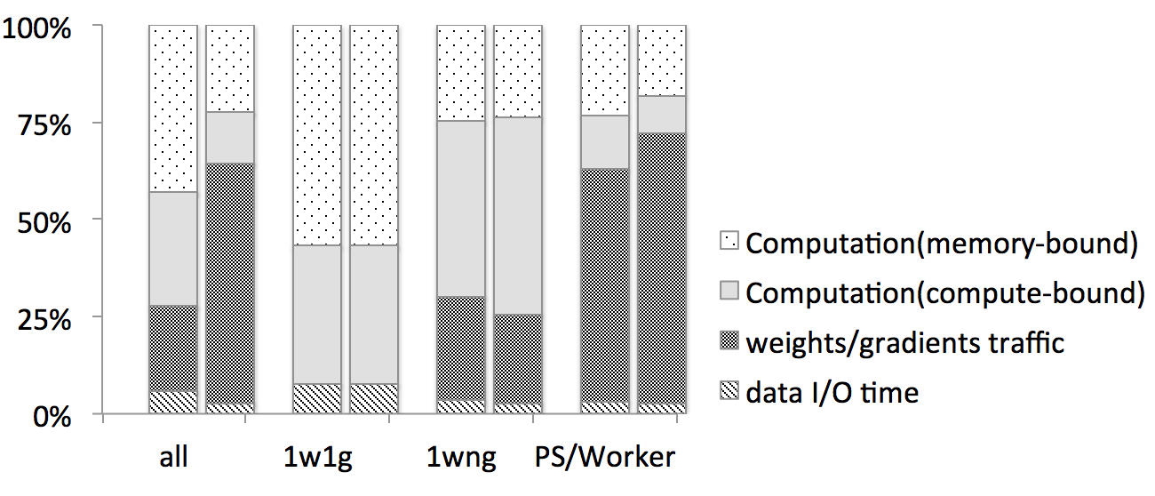
Figure 7: Average percentage of different parts of workload execution time. Left column: job-level, Right column: cNode-level.

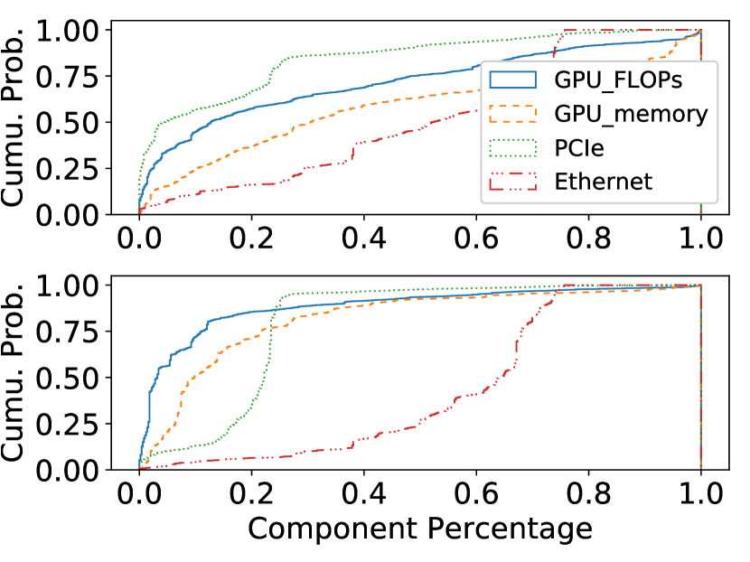
(a) all

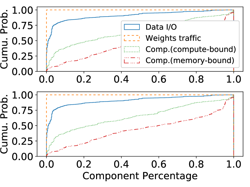
(b) 1w1g

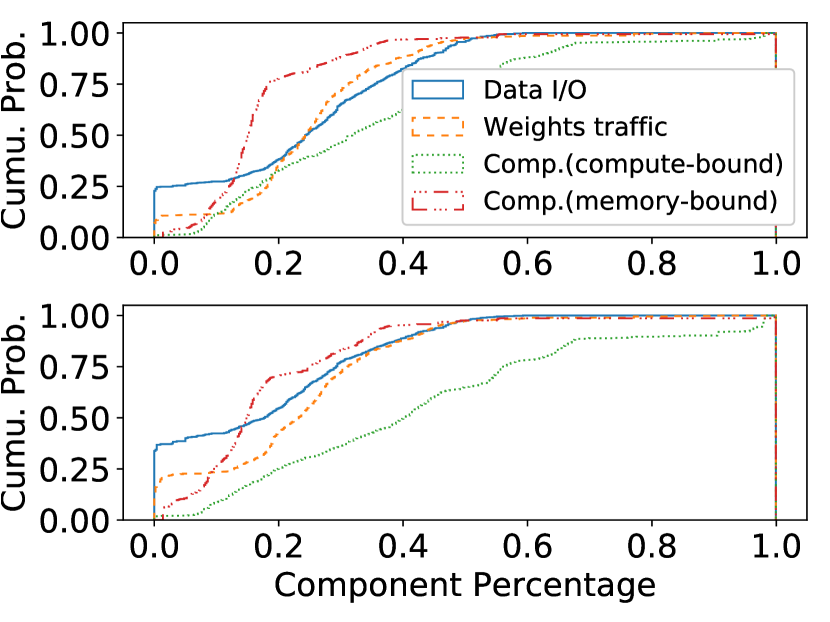
(c) 1wng

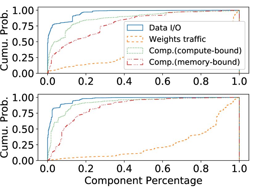
(d) PS/Worker

Figure 8: CDF of each component of the execution time among different workloads. Top: CDF at job-level, down: cNode-level.

III-B Performance Breakdown

Figure 7 shows the execution time breakdown for various workloads, including time for input data I/O, weight/gradient transfer and computation. The cNode-level percentages are computed as weighted sum of the job-level percentages, with the weight being the cNode number of each job over the overall cNode number. Please note that 1w1g jobs do not need weight/gradient communication. Figure 8 shows the detailed CDF of each component of the execution time, among the jobs. As the mapping from execution time components to hardware differs in different types of workloads (such as the weight movement is carried out via different hardware as shown in Table II), we summarize the overall time breakdown according to time spent on different hardware components and show the results in Fig. 8(a).

Input Data I/O. Figure 8 shows that for 1wng and PS/Worker workloads, input data movement time can be nearly ignored, approximately about 3% on average, partially because the weight/gradient transfer time is too large. One thing to note is that when such workloads are mapped to another system architecture or using a different hardware configuration, the bottleneck may shift, exposing the data I/O part, which will be illustrated in Sec. III-C.

For 1w1g workloads, the data I/O part is about 10% on average. Especially, there are about 5% of the workloads spending more than 50% time on input data movement, in which case the data I/O load on PCIe becomes the bottleneck.

Weight/Gradient Transfer. On average, weight/gradient communication contributes approximately 22% to the total execution time. When evaluating the percentage in the cNode-level, the proportion will be more than 60%, indicating that workloads with larger cNode numbers are more likely to suffer from the communication bottleneck. This can also be shown from the CDF of time breakdown of PS/Worker workloads in Fig. 8(d). The PS/Worker workloads always involve large numbers of cNodes with large proportions of time spent on weight/gradient transfer. Specifically, more than 40% PS/Worker jobs spend more than 80% time in communication via Ethernet and/or PCIe. Given the high communication overhead, a potential improvement to expedite model training is to upgrade the network facility or to vary the system configuration by porting the PS/Worker workloads to AllReduce-Local for leveraging the high communication efficiency introduced by NVLink.

Computation. Computation can be further decomposed into memory-bound and compute-bound computation. We can see that memory-bound computation time is larger than compute-bound operation time in all types of workloads. This indicates that the workloads in our cluster involve more memory access. In this case, XLA may provide powerful optimization for element-wise operations (major contribution for memory access). XLA is a domain-specific compiler for linear algebra that optimizes TensorFlow computation, which can fuse pipelined operations to reduce the memory overhead.

Additionally, for compute-bound operations, mixed-precision computation can also be introduced to exploit the computation power provided by TensorCore [23], which provides up to 8X higher peak FLOPS on Tesla V100, as compared to using standard FP32 operations on V100.

III-C Exploring the Optimization Space

Previously we showed a holistic execution profile for all workloads. But how would this execution profile change under different system settings? For instance, what can we get by upgrading the network bandwidth from 25Gbps to 100Gbps? Is there any further end-to-end performance speed-up by boosting the GPU peak computing power to 64 or 256 TFLOPS? Will the performance bottleneck shift to data movement by increasing GPU memory bandwidth to 4TB per second? In addition, what if we use AllReduce-Local or AllReduce-Cluster to run the PS jobs?

Next, we analytically evaluate potential performance impact by switching the PS workloads to AllReduce and by changing system configurations for different types of workloads. Especially, we estimate how the performance will be like when GPUs are upgraded to more powerful ones, and interconnections are varied among PCIe (for CPU-GPU/GPU-GPU communication), Ethernet (for cross-server communication), and NVLink (for high-speed inter-GPU communication within a single machine), by changing the values of $S_{d}$/$S_{w}$/$S_{mem_{access}}$/$peak_{FLOPs}$ in the analytical models in Sec. II-B, respectively. Tallent et al. [38] compared workload performance for GPU interconnect with NVLink and Cirrascale GX8 PCIe, and their results show that DGX-1 with NVLink has superior performance except on ResNet-type of workloads. We would like to investigate how much the high-speed NVLink interconnect can outperform PCIe/Ethernet with our workloads.

III-C1 Performance Impact of AllReduce

Figure 7 shows that communication consumes an important portion of the execution time in PS/Worker workloads, which may partially be due to the limited bandwidth of Ethernet/PCIe. We estiamte the performance when PS workloads training small to medium scale models (that can be fit into the GPU memory entirely) are ported to the AllReduce architectures, to exploit the high-speed NVLink. In addition to single node performance, we further evaluate the overall throughput of a training job, which can be computed as

$$throughput=\frac{\#cNode}{T_{total}}\times batch\_size$$ (2)

Here $\frac{\#cNode}{T_{total}}$ is the number of steps the job can train in unit time with all its computation nodes. Considering that $batch\_size$ remains the same in each computation node, the throughput is related to 1) single-node performance $T_{total}$ and 2) the number of cNodes $\#cNode$.

We map the PS/Worker workloads to the AllReduce-Local architecture as follows, since an AllReduce-Local job can have at most 8 $\#cNodes$: for a PS/Worker job with $\#cNodes>8$, the number of cNodes is reduced to 8; for those with $\#cNodes\leq 8$, the cNode numbers will remain unchanged. To map the PS/Worker workloads to the AllReduce-Cluster architecture, we retain the original number of cNodes in the jobs. In addition to the speedup of all workloads, we select workloads whose throughput cannot be improved by AllReduce-Local and show the performance acceleration with AllReduce-Cluster.

(a) AllReduce-Local

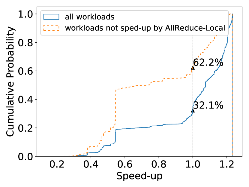
(b) AllReduce-Cluster

Figure 9: Improvement by mapping the workloads to AllReduce.

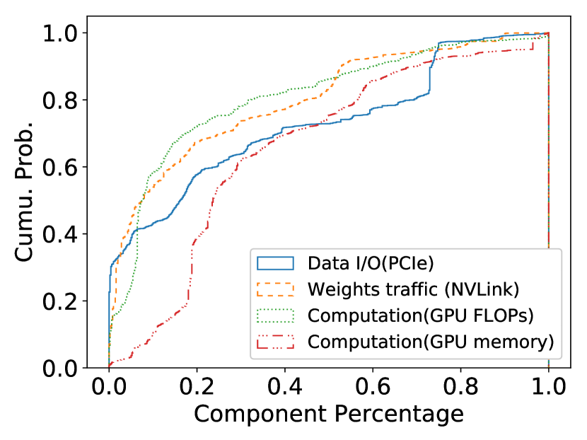
(a) CDF

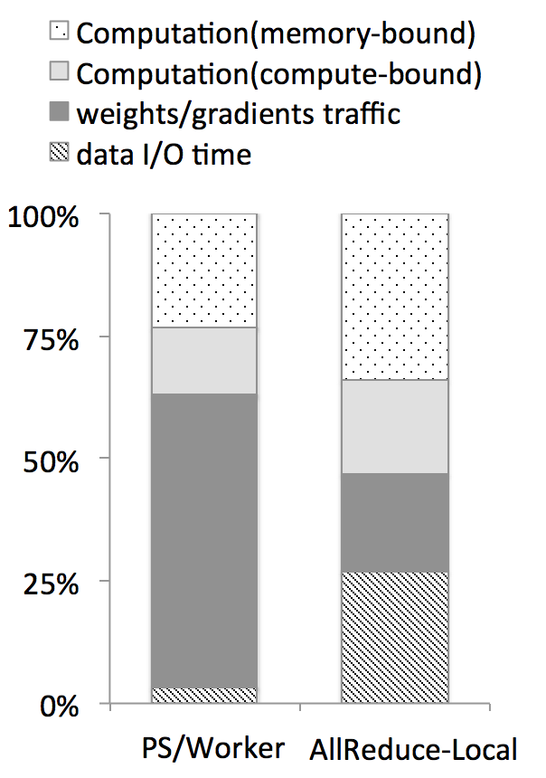
(b) Average Breakdown

Figure 10: Performance breakdown of PS/Worker workloads after being mapped to AllReduce-Local.

Fig. 9 shows that by shifting the communication medium from PCIe/Ethernet to the high speed NVLink interconnect with AllReduce-Local, most of the workloads can be accelerated at different levels. Considering the potential reduction of $\#cNode$ in projection, about 60% workloads still achieve speedup in the overall throughput. This indicates that AllReduce-Local architecture equipped with NVLink can potentially boost performance for most of the PS/Worker workloads, while at the same time saving system resources significantly (as the number of cNodes after projection will be no more than 8, which can be much larger before projection as shown in Fig. 6(a)). We also note that about 22.6% PS/Worker workloads cannot benefit from switching to the AllReduce-Local architecture. With the switching, all workloads experience acceleration of the weight/gradient transfer, as well as slow-down of input data I/O, due to the competition for PCIe bandwidth (as input data are transferred from CPU to multiple GPUs within a server simultaneously); whether a workload is sped up or slowed down relies on which part dominates.

To demonstrate the bottleneck shift effect, we further illustrate the execution time breakdown of the AllReduce-Local workloads in Fig. 10. As compared to the CDF shown in Fig. 8(d), we can observe that the weight/gradient communication part is vastly reduced, while the other parts, including computation and the data I/O fraction, become more important. Especially, based on Fig. 10(b), we can see that the portion of data I/O via PCIe increases the most, indicating the shift of bottlenecks with different architectures.

When workloads are shifted from PS/Worker to AllReduce-Cluster, the main speedup is due to the change of weight/gradient movement medium from Ethernet&PCIe to Ethernet&NVLink. However, in both sets of configurations, Ethernet is the main bottleneck for data transfer, and thus the speedup is quite limited, at most 1.2X based on Table I. On average, 67.9% workloads can be sped up. Furthermore, among the workloads that cannot be improved by AllReduce-Local, about 37.8% can be sped up with AllReduce-Cluster.

TABLE III: Hardware Configuration Variations

	Candidates
Ethernet/Gbps	{10, 25, 100}
PCI/GB	{10, 50}
GPU peak FLOPs/T	{8, 16, 32, 64}
GPU memory/TB	{1, 2, 4}

III-C2 Performance Impact of Hardware Evolution

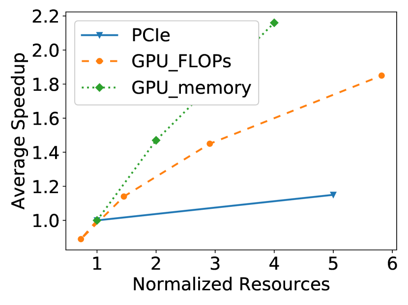
(a) 1w1g

(b) 1wng

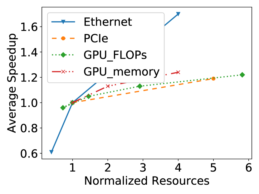
(c) PS/Worker

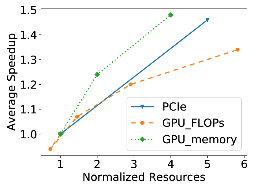
(d) AllReduce-Local

Figure 11: Speedup with different hardware configurations.

We next investigate how the workloads perform with different hardware configurations, as shown in Table III. We show normalized resource values in Fig. 11 according to the basic settings in Table I, to facilitate result comparison. For example, the Ethernet bandwidth is normalized using 25Gbps as the basic unit, and PCIe bandwidth is normalized by 10GB/s. We evaluate both the original workloads with 1w1g, 1wng and PS/Worker architectures, and also the mapped AllReduce-Local workloads from the PS/Worker workloads.

In Fig. 11, the speedup is computed using the performance achieved with the new configuration of the respective resource. Different workloads exhibit different behaviors: 1w1g workloads are most sensitive to GPU memory bandwidth, 1wng ones vary most with the variation of PCIe bandwidth, and the PS/Worker type relies most on the Ethernet bandwidth. The observations are consistent with the performance breakdown results in Fig. 7 and Fig. 8. For example, PS/Worker workloads spend the most time on weight/gradient transfer via Ethernet and they achieve the highest speedup by improvement of the Ethernet bandwidth.

Comparison between Fig. 11(c) and (d) shows the bottleneck shift effect: performance of PS/Worker workloads varies most when varying the Ethernet bandwidth, and they are accelerated quite a bit when the GPU memory bandwidth improves; when the workloads are projected to AllReduce-Local, GPU memory bandwidth has the largest impact on performance.

III-D Summary of Key Observations

We make several interesting observations based on the above:

$\triangleright$ On PAI, distributed training jobs dominate resource consumption, with PS/Worker jobs consuming 81% of overall computation resources.

$\triangleright$ 90% jobs train small-scale models, i.e., model size less than 10GB, while there exist also large-scale models(100-300GB) which are trained in large-scale distributed mode and consumes large amounts of resources.

$\triangleright$ On average weight/gradient communication takes almost 62% of the total execution time for all workloads. For PS/Worker jobs, more than 40% workloads spend more than 80% time in weight/gradient communication. As to the computation portion which is the focus of previous studies [16, 39], on average it only contributes 35% of the total training time, with compute-bound part contributing 13% and memory-bound part 22%.

$\triangleright$ Throughput of 60% PS/Worker workloads can be improved when they are ported to the AllReduce-Local architecture, which can leverage the high-speed NVLink for GPU interconnect.

$\triangleright$ Workloads show different levels of sensitivity for hardware evolution and the performance bottleneck may shift with the change of system architecture. PS/Worker workloads are most sensitive to Ethernet bandwidth; after projected to AllReduce-Local, they benefit the most from the improvement of GPU memory access bandwidth.

IV Performance Characterization: Case Studies

In this section, we zoom into the training of several production DL models in detail, to further detect their performance bottlenecks and evaluate several optimization techniques.

We run the selected training workloads in an experimental testbed of 64 servers. Each server is equipped with one 96-core Intel Xeon Platinum 8163 CPU, eight Tesla V100 GPUs, 128GB RAM, 10GB PCIe and 50GB NVLink. The servers are connected through 25Gbps bi-directional Ethernet. We extensively investigate data preprocessing time and the framework overhead (mostly due to CPU runtime scheduling and GPU kernel launch time), which are not considered in Sec. III as they are not fundamental resource demands of workloads and can be optimized to be ignorable using different technologies. With our testbed experiments, we will show the impact of the framework overhead and discuss techniques to minimize it.

IV-A Selected Workloads

Table IV summarizes the six models used for our case studies, selected from different application domains and with different scales of parameter size.

ResNet50. Residual networks have been proven to be powerful and widely applied in multiple domains [2, 40].

NMT. In our production system, NMT model [41] has been applied to translation for e-commerce business and others.

Speech. Neural acoustic models [42] have been useful in speech recognition and widely adopted in commercial acoustic applications. The model we evaluate is composed of CNN followed by Long Short-Term Memory (LSTM) architecture with layer normalization.

BERT. BERT [6] is one of the most commonly used models for language understanding, and has been applied to a few business domains in our company.

Multi-Interests. Multi-interest model [43, 44] based recommender systems are widely used in our service platform, to capture users’ various interests.

GCN. GCN (Graph Convolutional neural Network) [9, 10] is based on a well-known graph embedding framework. The item embeddings are employed to compute pairwise similarities between all items to facilitate recommendation.

TABLE IV: Model Scale

	Domain	Dense	Embedding	System
		weights	weights	Architecture
ResNet50	CV	204MB	0MB	AllReduce-Local
NMT	Translation	706MB	819MB	AllReduce-Local
BERT	QA	1GB	284MB	AllReduce-Local
Speech	Speech recognition	416MB	0MB	1w1g
Multi-Interests	Recommender	1.19MB	239.45GB	PS/Worker
GCN	Recommender	207MB	54GB	PEARL

Table IV summarizes the parameter sizes for the models, including dense weights and embedding weights [9]. Note that the parameter sizes include both the trainable variables and the optimization-related variables, such as momentums [45]. For models with small weight size (such as ResNet50, NMT and BERT), all parameters can concurrently reside in the GPU memory; hence AllReduce-Local architecture is adopted for their training, to leverage GPU-direct technology (NVLink). For models with large-scale weights (such as Multi-Interests), only the PS/Worker architecture is suitable, as the weight size supported by the current AllReduce frameworks is limited by single GPU’s memory size.

In our testbed, we train each model using the system architecture indicated in Table IV. The Speech model evaluated is only trained on a small dataset, so does not require distributed training and is trained using 1w1g. For GCN with a large model size, we will show that the limited Ethernet bandwidth becomes the bottleneck when PS/worker architecture is used, and we will design a new system architecture (PEARL) for its training. Table V shows the basic workload features.

TABLE V: Basic Workload Features

	Batch Size	FLOP count	Memory access	Memory Copy(PCIe)	Network Traffic
Multi-Interests	2048	105.8G	100.4GB	261MB	122MB
ResNet50	64	1.56T	31.9GB	38MB	357MB
NMT	6144	2.5T	101.6GB	22KB	1.33GB
BERT	12	2.1T	107.3GB	46KB	1.5GB
Speech	32	7.9T	20.4GB	804MB	728MB
GCN	512	330.7G	25.79GB	1.2MB	3GB

IV-B Model Validation

We first compare the execution time breakdown estimated using the analytical models in Sec. II-B and the actual measurement results. For example, ResNet50 involves 1.56T FLOPs, while the peak computing FLOPs provided by Tesla V100 in our testbed is 15 TFLOPs; thus, the compute-bound computation time is predicted via $\frac{1.56}{15*70\%}=0.149s$, where 70% is the basic assumption for hardware utilization efficiency. The actual measured time for this part is 0.126s. Similar estimation method is used to other parts, including data I/O, weight/gradient traffic time, etc. The estimated time and the actual measurement time, and even the time composition, are used in comparison for model validation.

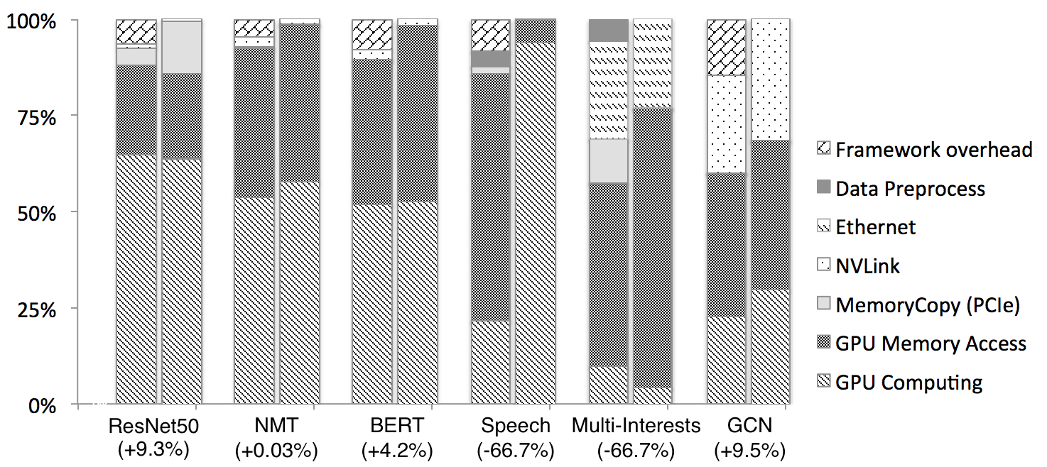
Figure 12: Time Breakdown Comparison. Left: actual measurement, right: estimation.

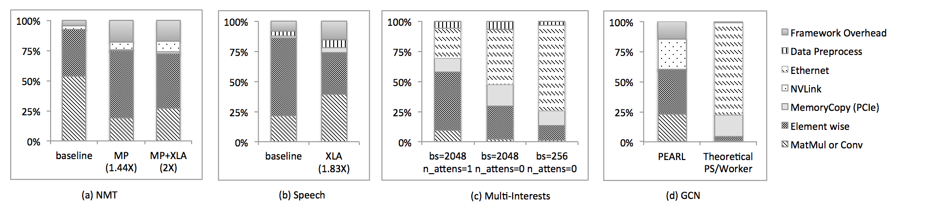
Figure 13: Performance Breakdown with Different Optimization Techniques.

In Fig. 12, the percentage in the parentheses indicates the time difference, computed as $\frac{T_{predict}-T_{actual}}{T_{actual}}$, where $T_{predict}$ is the total time we estimated and $T_{actual}$ is the actual measured time. The difference is less than 10% in most cases, and the estimated time breakdown can quite accurately reflect the relative portions of computation and data transfer in the entire execution time. For the Speech model, the difference is more than 66.7%. Our estimation inaccuracy is due to the actual low usage of GPU memory access bandwidth at only 3%, much smaller than the 70% assumption when we do the estimation. We seek how to further improve memory access efficiency as a future direction, while adopting possible optimization such as XLA to reduce the memory-access volume by operation fusion, to accelerate training of the Speech model.

IV-C PEARL Architecture

Used in the domain of e-commerce, search and recommendation models have very large and sparse commodity-embedding parameters. When the model size (ranging from tens to hundreds of GB) is too large to fit into the GPU memory entirely, the PS/Worker architecture should be adopted to partition and store the variables in the CPU memory among multiple PS nodes. However, synchronizing a large variable among the PS and GPUs of the workers requires significant ethernet and PCIe bandwidth, and also consumes many CPU clocks.

Parameters of such models can be classified into dense and sparse weights, depending on how their elements are accessed. Treating the whole model as dense is inefficient, since naïvely communicating all elements of a large sparse variable, even though only a small subset is accessed, results in relatively low scalability.

We propose and implement PEARL (Partitioned Embedding And RepLicated), a new distribution strategy that optimizes the efficiency of data transfer by taking the sparsity of variables into account.

As shown in Fig. 14, PEARL applies a hybrid approach that partitions the large sparse variables and distributes them in the GPU memory of workers, and adopts the AllReduce architecture to process dense variables.

All workers synchronize variables via collective communication operations such as AllReduce and AllGatherv. AllReduce aggregates gradients from all GPUs for the dense weights, while AllGatherv gathers the embedding weights and corresponding gradients from all GPUs for the partitioned weights. The AllGatherv operation is implemented on top of NCCL [34] primitives such as Broadcast and Reduce, that are optimized to leverage high-speed inter-GPU NVLink.

Experiments show that PEARL built atop TensorFlow achieves good scalability in terms of training throughput with the increase of computation resources, on both dense and sparse models.

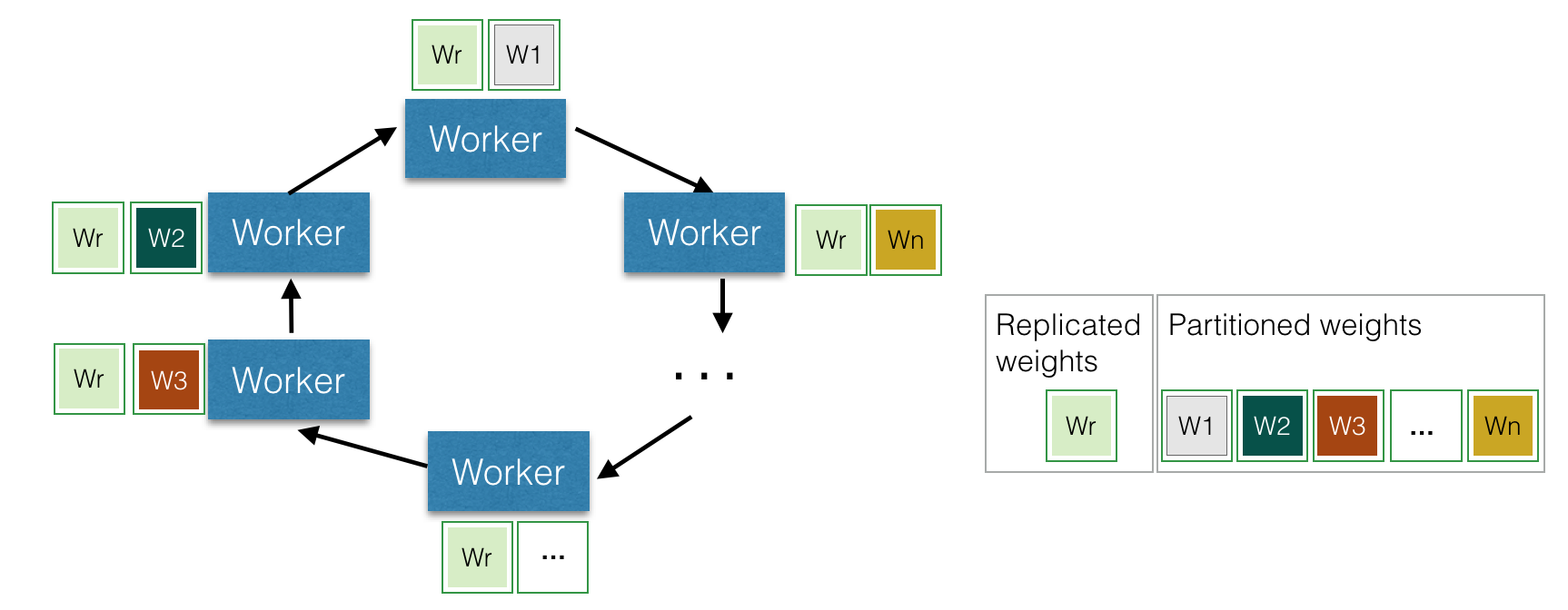
Figure 14: Architecture of PEARL.

IV-D Effectiveness of Optimization Techniques

As shown in Fig. 12, behavior of ResNet50, NMT and BERT is quite similar: 1) the actual time measurements and the model-based estimation are close, indicating that the hardware usage efficiency is quite high, around the basic assumption of 70%. 2) the computation part contributes the most to the total running time, which shows that the communication part of time is reduced quite well by using NVLink.

We next investigate how to further improve the computation efficiency. Fig. 13(a) compares the results obtained using the default setting, with mixed-precision (MP) matrix multiplication in FP16 [46] enabled (which is available with TensorCore in Volta architecture, potentially achieving up to 8X speedup compared to the default multiply-and-addition in FP32), and with XLA enforced. We observe 1.44X end-to-end speedup and 2.8X for MatMul when mixed-precision optimization is in use. With the powerful tool XLA (operation fusion and code generation), element-wise operation time can be reduced, as operation fusion exploits GPU’s high-speed cache to reduce the framework scheduling overhead. We observe 2X speedup with both MP and XLA in place (1.76X with only XLA).

Fig. 13(b) shows that when using XLA when training the Speech model, 3.43X speedup can be achieved for element-wise operations and 1.83X for the end-to-end performance.

Figure 13(c) presents the time breakdown of Multi-Interests model training under three different training configurations (batch size and the number of attention layers). With the same model, performance bottlenecks in case of different configurations vary significantly. Larger batch size is more friendly to GPU with element-wise operations being the bottleneck, whose computation time can be reduced by operation fusion at the runtime. With the third configuration, communication becomes the bottleneck. A Multi-Interests model has a large weight size of more than 200GB; the weights cannot be entirely stored in the GPU memory. Therefore, we cannot apply the AllReduce architecture to leverage the high-speed NVLink (since current AllReduce frameworks only support weight-replica mode). Similarly, GCN has large-scale embedding weights, and PS/Worker framework should be used. However, large-volume communication via Ethernet and PCIe may become the bottleneck. In these cases, PEARL is applied, which can use NVLink to transfer the weights/gradients for large-scale models, is in need.

With PEARL, the large-scale weights, such as embeddings, are partitioned among multiple GPUs, while the variable/gradient aggregation is performed using a PS/Worker like protocol, using AllGather and ReduceScatter operations [34]; all other small-scale weights are replicated and AllReduce is used for gradient exchange. Fig. 13(d) presents the time breakdown of GCN model when trained using PEARL. We see that with the high-speed interconnect, the communication part via NVLink consumes 25% of the total time. Using our analytical approach, we can also estimate the time breakdown when using PS/Worker with Ethernet & PCIe for training, which is shown in the second bar in Fig. 13(d). The communication part with Ethernet & PCIe contributes to almost 95% of the total time, which is much more than what we can achieve with PEARL.

V Discussions

In our proposed workload characterization framework, there are several assumptions that may affect the results. In this section, we discuss the effects when the assumptions shift.

V-A Hardware efficiency assumption

As described in Sec. II-B, the hardware efficiencies of computation (GPU) and communication (PCIe/Ethernet/NVLink) parts are both assumed to be 70%. To find out whether the assumption is reasonable, we conduct cross-validation in two ways. First, we measure the hardware efficiency in each case analyzed in Sec. IV. Next, as it is sophisticated to establish a system to precisely measure the hardware utility efficiency for each workload, instead we try to analyze how the results will shift if the assumption is not followed.

Table VI shows the actual measured hardware efficiency for each workload. 70% is about the average level. In detail, we can observe that, the efficiency of GPU computation/ memory access is a bit higher than 70%, while that of data traffic (PCIe/Ethernet/NVlink) is lower.

TABLE VI: Resource Efficiency for Each Workload

	GPU TOPS	GDDR	PCIe	Network (Ethernet/NVLink)
Multi-Interests	32.71%	95%	86.47%	69.21%
ResNet50	82.55%	78.9%	35.1%	49.4%
NMT	82.8%	79.1%	0.1%	35.2%
BERT	81.6%	95%	0.42%	47.1%
Audio	60.86%	3.1%	77.73%	40.5%
GCN	88.2%	69.9%	86.2%	27.35%

For the collective behavior, we explore how the conclusion will change if the assumption is violated. Taking PS/Worker workloads as example, we evaluate how the weight traffic’s portion in the end-to-end training time varies when the hardware efficiency in computation/communication changes. As shown in Fig. 15, as expected, when the actual hardware efficiency in communication (PCIe/Ethernet) is lower than 70%, the PS/Worker workloads will spend more time on weight traffic, and vice versa. What should be noted is that even when the hardware efficiency in computation is only 25% (quite lower than the 70% assumption), the PS/Worker workloads still spend more time on weight traffic on average.

To give a precise estimation on the fundamental bottleneck in the cluster using our proposed framework, it is still important to establish a better methodology to measure the utilization efficiency of each hardware component, which will be an important direction in our future work.

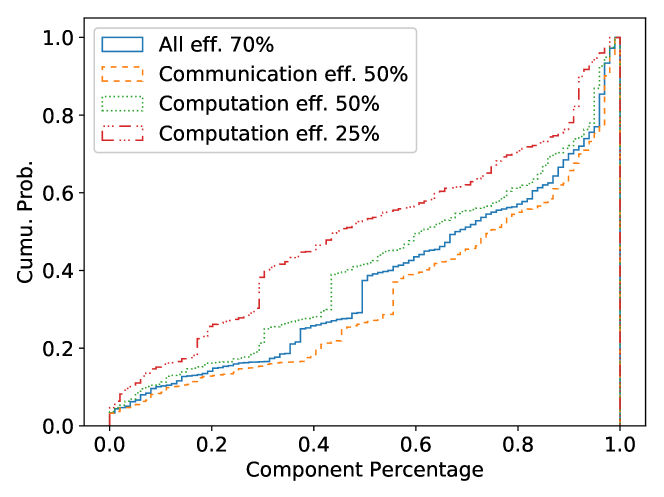
Figure 15: Shift Effect in Weight Traffic Percentage When Hardware Efficiency Changes.

V-B Computation/communication overlap assumption

There are various ways to overlap computation and data transfer [36, 37] in DL workloads. Although the purpose of this work is to expose the fundamental performance bottlenecks, which will not change due to the overlap issue, several speedup results may change if the non-overlap assumption is violated. As how to achieve computation and communication overlap is still an open question in deep learning design, it is not easy to quantify the actual overlap potential for each workload. Instead, we use an ideal overlap case to give an estimation for comparison. In this case, the total time changes from $T_{total}=T_{d}+T_{c}+T_{w}$ (used in our framework in Sec. II-B) to $T_{total}=\max\{T_{d},T_{c},T_{w}\}$.

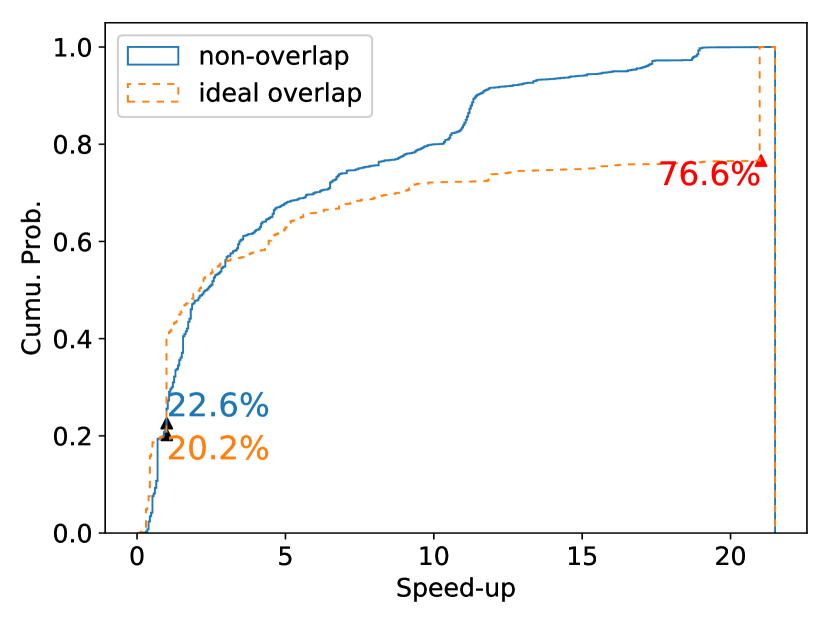
Figure 16: Shift Effect Under Different Overlap States. Left: weight traffic percent, right: speedup when mapping to AllReduce-Local

Fig. 16 shows the comparison results of PS/Worker workloads under different overlap states: totally none-overlap VS ideal-overlap. It can be observed that when computation and communication ideally overlap, the weight traffic part is heavily exposed as the performance bottleneck, as it consumes the longest time among $\{T_{d},T_{c},T_{w}\}$. As to the speedup analysis when mapping PS/Worker workloads to the AllReduce-Local architecture, we can observe that the ratio of sped-up workloads remains similar as the none-overlap results, 22.6% VS 20.2%. It can be noted that there are 23.4% workloads achieving 21X speedup, which are actually the workloads bound by the weight traffic part either before or after the architecture projection. For such workloads, the speedup ratio can be computed as:

$$\frac{\frac{S_{w}}{25Gb\times 70\%}+\frac{S_{w}}{10GB\times 70\%}}{\frac{S_{w}}{10GB\times 70\%}}=21$$ (3)

where $S_{w}$ denotes the weight traffic volume.

The comparison further illustrates that the assumption of computation/communication overlap may affect the detailed analytical results, such as speedup ratio or running time constitution; however, it does not change the conclusion as to what is the fundamental bottleneck for the workloads in our cluster. At last, it is worth noting that the purpose of our analysis framework is not to precisely predict practical performance of workloads, but to expose the fundamental bottlenecks in hardware components or system architecture for collective behavior of workloads in our cluster.

VI System Implications

Based on previous results, we now summarize important implications on how to optimize training frameworks (e.g. TensorFlow) and how to properly provision system resources.

VI-A Implications on Framework Optimization

VI-A1 System Architecture

In the PAI cluster, we identified plenty of DL models that are not suitable to be trained using either PS/Worker or AllReduce, e.g., models with one large sparse embedding and many relatively small dense weights (such as GCN in Section IV). The weight sizes within such workloads are too large to be resident in GPU memory. On the other hand, such workloads always incur heavy weight/gradient traffic, for which the Ethernet connections with limited bandwidth will be the bottleneck. For such workloads, we proposed a new strategy PEARL, as inspired by our characterization of collective behavior in the cluster, catering to the resource requirements of such workloads.

Our simple analytical model can predict the time breakdown of jobs on different architectures, facilitating system architecture selection. Though our model does not take potential framework overhead into consideration, experiments show that its estimation is quite close to real measurements for representative workloads. A more comprehensive prediction method is one of our future directions to explore.

VI-A2 Compilation: Operation Fusion and Code Generation

Statistical results in Sec. III show that, within the computation part, the time spent on memory-bound operations is no less than that of computation-bound ones. TensorFlow XLA is a solid compilation framework for operation fusion and code generation to reduce the memory accesses. We have shown that XLA is powerful enough to handle practical training workloads. As shown in Sec. IV, different workloads have drastically different computation profiles. For ResNet50, NMT and BERT, memory-access time takes at most 40% of execution time. In large-scale recommendation models (Multi-Interests, GCN), it takes up to 60%. For all these workloads, compilation using XLA is helpful in reducing CPU launch overhead and improving GPU computation efficiency.

XLA is known to have several limitations. For example, it cannot deal well with workloads with dynamic shapes, the operation fusion algorithm is designed as rule-based and cannot be generalized well, the code generation mechanism still needs to be improved to generate highly optimized kernels [47]. The community is calling for a powerful, robust compilation infrastructure that is able to handle rapidly changing training workloads in the future.

VI-A3 Framework Overhead

Frameworks like TensorFlow use a flexible and general enough CPU runtime to do computation scheduling. If the main part of the computation graph consists of very fine-grained operations, CPU scheduling may incur non-negligible overheads, especially in busy CPU/GPU clusters with a mixture of workloads deployed.

Most of our workloads have regular computation structures, and carry out repetitive iterations during the training process. Through compilation (discussed above), it is possible to allow a larger portion of the computation graph to be scheduled to the GPU altogether.

VI-B Implications on Hardware Configurations

VI-B1 Interconnect Bandwidth

There are two types of interconnects for distributed training in our cluster: NVLink and Ethernet, with notable gap w.r.t. the communication bandwidth. We have shown the performance gain of high speed interconnects for weight/gradient communication in numerous medium scale ($<$50GB) workloads. For large models (e.g. Multi-Interests model in Sec. IV), weight/gradient communication over the Ethernet can take up to more than 50% of execution time per iteration. High-bandwidth interconnects will definitely help such communication-bound workloads, as shown in Fig. 11.

VI-B2 PCIe Bandwidth

In our system settings, PCIe is mainly dedicated for data transfer between CPU and GPU. In distributed training, PCIe traffic normally consists of two portions: sample data input, and weight/gradient communication. As shown in Sec. III, in most workloads, the sample input volume is negligible, and weight/gradient transfer is usually bound by network rather than PCIe.

However, this does not mean that PCIe bandwidth is less important for performance. As shown in Fig. 10, the bottleneck may be shifted to PCIe after the network bandwidth usage is optimized. Additionally, high-speed PCIe interconnects can enable exciting new optimization opportunities for some mission critical applications. The basic idea is to push as much work as possible, from CPU to GPU, in order to allow more operations in the computation graph to be processed in GPU as a whole and minimize CPU intervention.

VI-B3 GPU Computing Power and Memory Bandwidth

Computing power and memory bandwidth of GPUs are essential for DL workloads. Important as they are, we have shown in Sec. III that weight/gradient communication renders the biggest performance bottleneck in our cluster. More careful model distribution and system architecture selection are necessary to mitigate communication overhead in order to fully exploit the computation power.

VII Related Work

There have recently been several studies conducting cluster-level machine learning workload characterization, aiming to improve resource utilization and workload performance in the ML cluster [20, 48, 49]. Park et al. [20] analyze the inference workloads in a Facebook data center, pointing out limitations of the current ML infrastructure [19] and providing suggestions for future general-purpose/accelerated inference hardware. Jeon et al. [48] present a detailed workload characterization of a two-month trace from a multi-tenant GPU cluster, and focused on resource utilization and scheduling.

Some other work aim to establish the performance benchmark [22, 16, 50, 18]. Fathom [16] establishes a set of reference implementation for eight archetypal DL jobs. Guignard et al. [51] adopt the eight types of workloads from Fathom to evaluate the performance of the IBM “Minsky” platform. A micro-benchmark is designed in [52] to measure reads in TensorFlow and a burst buffer is implemented to improve the I/O performance. Gao et al. [50, 18] establish a proxy benchmark for AI workloads by identifying eight data motifs.

Several studies have focused on predicting the performance of a job using a mathematical model [39, 15, 53, 54]. PALEO [39] establishes a performance model by extracting the basic computational requirements and mapping them to a specific point within the design space of software, hardware and communication strategies. DeepProf [15] is a tool that can automatically process GPU traces and generate performance reports for deep learning applications, which can perform diagnosis to identify the runtime bottleneck. The above two work both aim to break down the execution time of a workload, with the former analyzing from the theoretical perspective and the latter using runtime traces. Ernest [53] builds a performance model from the workload observation on small datasets and predicts the performance on larger datasets in bigger clusters. Justus et al. [55] predict execution time of one part in the entire DL network; execution time of the sub-graph constitutes a basic unit for predicting the end-to-end performance.

Different from the existing work that aim at precisely predicting practical performance of a given workload, our work focuses on characterization of currently deployed jobs on our large cluster and extracting their fundamental resource requirements, in order to expose the potential hardware/software optimization directions at the cluster scale. From our observations, we extract fundamental execution bottlenecks and identify latent, useful directions for training framework optimization or system configuration improvement.

VIII Conclusion

This paper presents a characterization framework to enable performance analysis over diversified production workloads running on Alibaba-PAI. The framework features a lightweight technique to collect runtime profiling metrics of workloads. Based on collected job statistics, we build a workload model to extract key features and project them to different system configurations in order to analytically predict the performance behavior. We characterize collective behavior of a large volume of workloads, as well as zoom into representative workloads for investigating impact of different system architectures and hardware configurations. We discuss potential technical directions for improving training performance of the workloads. As future work, we seek to characterize inference workloads in our cluster using a similar methodology.

References

- [1] Alex Krizhevsky, Ilya Sutskever, and Geoffrey E Hinton. Imagenet classification with deep convolutional neural networks. In Advances in neural information processing systems, pages 1097–1105, 2012.
- [2] Kaiming He, Xiangyu Zhang, Shaoqing Ren, and Jian Sun. Identity mappings in deep residual networks. In European conference on computer vision, pages 630–645. Springer, 2016.
- [3] Andrej Karpathy, George Toderici, Sanketh Shetty, Thomas Leung, Rahul Sukthankar, and Li Fei-Fei. Large-scale video classification with convolutional neural networks. In Proceedings of the IEEE conference on Computer Vision and Pattern Recognition, pages 1725–1732, 2014.
- [4] Karen Simonyan and Andrew Zisserman. Two-stream convolutional networks for action recognition in videos. In Advances in neural information processing systems, pages 568–576, 2014.
- [5] Dzmitry Bahdanau, Kyunghyun Cho, and Yoshua Bengio. Neural machine translation by jointly learning to align and translate. arXiv preprint arXiv:1409.0473, 2014.
- [6] Jacob Devlin, Ming-Wei Chang, Kenton Lee, and Kristina Toutanova. Bert: Pre-training of deep bidirectional transformers for language understanding. arXiv preprint arXiv:1810.04805, 2018.
- [7] Alex Graves, Abdel-rahman Mohamed, and Geoffrey Hinton. Speech recognition with deep recurrent neural networks. In 2013 IEEE international conference on acoustics, speech and signal processing, pages 6645–6649. IEEE, 2013.
- [8] Jan K Chorowski, Dzmitry Bahdanau, Dmitriy Serdyuk, Kyunghyun Cho, and Yoshua Bengio. Attention-based models for speech recognition. In Advances in neural information processing systems, pages 577–585, 2015.
- [9] Jizhe Wang, Pipei Huang, Huan Zhao, Zhibo Zhang, Binqiang Zhao, and Dik Lun Lee. Billion-scale commodity embedding for e-commerce recommendation in alibaba. In Proceedings of the 24th ACM SIGKDD International Conference on Knowledge Discovery & Data Mining, pages 839–848. ACM, 2018.
- [10] Rex Ying, Ruining He, Kaifeng Chen, Pong Eksombatchai, William L Hamilton, and Jure Leskovec. Graph convolutional neural networks for web-scale recommender systems. In Proceedings of the 24th ACM SIGKDD International Conference on Knowledge Discovery & Data Mining, pages 974–983. ACM, 2018.
- [11] Chenyi Chen, Ari Seff, Alain Kornhauser, and Jianxiong Xiao. Deepdriving: Learning affordance for direct perception in autonomous driving. In Proceedings of the IEEE International Conference on Computer Vision, pages 2722–2730, 2015.
- [12] David Silver, Aja Huang, Chris J Maddison, Arthur Guez, Laurent Sifre, George Van Den Driessche, Julian Schrittwieser, Ioannis Antonoglou, Veda Panneershelvam, Marc Lanctot, et al. Mastering the game of go with deep neural networks and tree search. nature, 529(7587):484, 2016.
- [13] Barret Zoph and Quoc V Le. Neural architecture search with reinforcement learning. arXiv preprint arXiv:1611.01578, 2016.
- [14] Shaohuai Shi, Qiang Wang, Pengfei Xu, and Xiaowen Chu. Benchmarking state-of-the-art deep learning software tools. In 2016 7th International Conference on Cloud Computing and Big Data (CCBD), pages 99–104. IEEE, 2016.
- [15] Jiazhen Gu, Huan Liu, Yangfan Zhou, and Xin Wang. Deepprof: Performance analysis for deep learning applications via mining gpu execution patterns. arXiv preprint arXiv:1707.03750, 2017.
- [16] Robert Adolf, Saketh Rama, Brandon Reagen, Gu-Yeon Wei, and David Brooks. Fathom: Reference workloads for modern deep learning methods. In 2016 IEEE International Symposium on Workload Characterization (IISWC), pages 1–10. IEEE, 2016.
- [17] Ang Li, Shuaiwen Leon Song, Jieyang Chen, Xu Liu, Nathan Tallent, and Kevin Barker. Tartan: Evaluating modern gpu interconnect via a multi-gpu benchmark suite. In 2018 IEEE International Symposium on Workload Characterization (IISWC), pages 191–202. IEEE, 2018.
- [18] Wanling Gao, Jianfeng Zhan, Lei Wang, Chunjie Luo, Zhen Jia, Daoyi Zheng, Chen Zheng, Xiwen He, Hainan Ye, Haibin Wang, et al. Data motif-based proxy benchmarks for big data and ai workloads. In 2018 IEEE International Symposium on Workload Characterization (IISWC), pages 48–58. IEEE, 2018.
- [19] Kim Hazelwood, Sarah Bird, David Brooks, Soumith Chintala, Utku Diril, Dmytro Dzhulgakov, Mohamed Fawzy, Bill Jia, Yangqing Jia, Aditya Kalro, et al. Applied machine learning at facebook: a datacenter infrastructure perspective. In 2018 IEEE International Symposium on High Performance Computer Architecture (HPCA), pages 620–629. IEEE, 2018.
- [20] Jongsoo Park, Maxim Naumov, Protonu Basu, Summer Deng, Aravind Kalaiah, Daya Khudia, James Law, Parth Malani, Andrey Malevich, Satish Nadathur, et al. Deep learning inference in facebook data centers: Characterization, performance optimizations and hardware implications. arXiv preprint arXiv:1811.09886, 2018.
- [21] Shaohuai Shi, Qiang Wang, and Xiaowen Chu. Performance modeling and evaluation of distributed deep learning frameworks on gpus. In 2018 IEEE 16th Intl Conf on Dependable, Autonomic and Secure Computing, 16th Intl Conf on Pervasive Intelligence and Computing, 4th Intl Conf on Big Data Intelligence and Computing and Cyber Science and Technology Congress (DASC/PiCom/DataCom/CyberSciTech), pages 949–957. IEEE, 2018.
- [22] Hongyu Zhu, Mohamed Akrout, Bojian Zheng, Andrew Pelegris, Anand Jayarajan, Amar Phanishayee, Bianca Schroeder, and Gennady Pekhimenko. Benchmarking and analyzing deep neural network training. In 2018 IEEE International Symposium on Workload Characterization (IISWC), pages 88–100. IEEE, 2018.
- [23] NVIDIA. Nvidia tesla v100 gpu architecture. https://images.nvidia.com/content/volta-architecture/pdf/volta-architecture-whitepaper.pdf, 2017.
- [24] The XLA Team. Xla – tensorflow compiled. post in the google developers blog. https://developers.googleblog.com/2017/03/xla-tensorflow-compiled.html, 2017.
- [25] Martín Abadi, Paul Barham, Jianmin Chen, Zhifeng Chen, Andy Davis, Jeffrey Dean, Matthieu Devin, Sanjay Ghemawat, Geoffrey Irving, Michael Isard, et al. Tensorflow: A system for large-scale machine learning. In 12th USENIX Symposium on Operating Systems Design and Implementation (OSDI 16), pages 265–283, 2016.
- [26] Yangqing Jia, Evan Shelhamer, Jeff Donahue, Sergey Karayev, Jonathan Long, Ross Girshick, Sergio Guadarrama, and Trevor Darrell. Caffe: Convolutional architecture for fast feature embedding. In Proceedings of the 22nd ACM international conference on Multimedia, pages 675–678. ACM, 2014.
- [27] Adam Paszke, Sam Gross, Soumith Chintala, Gregory Chanan, Edward Yang, Zachary DeVito, Zeming Lin, Alban Desmaison, Luca Antiga, and Adam Lerer. Automatic differentiation in pytorch. 2017.
- [28] Tianqi Chen, Mu Li, Yutian Li, Min Lin, Naiyan Wang, Minjie Wang, Tianjun Xiao, Bing Xu, Chiyuan Zhang, and Zheng Zhang. Mxnet: A flexible and efficient machine learning library for heterogeneous distributed systems. arXiv preprint arXiv:1512.01274, 2015.
- [29] Dong Yu, Adam Eversole, Mike Seltzer, Kaisheng Yao, Zhiheng Huang, Brian Guenter, Oleksii Kuchaiev, Yu Zhang, Frank Seide, Huaming Wang, et al. An introduction to computational networks and the computational network toolkit. Microsoft Technical Report MSR-TR-2014–112, 2014.
- [30] Nvlink. https://www.nvidia.com/en-gb/data-center/nvlink/.
- [31] Ruben Mayer and Hans-Arno Jacobsen. Scalable deep learning on distributed infrastructures: Challenges, techniques and tools. arXiv preprint arXiv:1903.11314, 2019.
- [32] Christopher J Shallue, Jaehoon Lee, Joe Antognini, Jascha Sohl-Dickstein, Roy Frostig, and George E Dahl. Measuring the effects of data parallelism on neural network training. arXiv preprint arXiv:1811.03600, 2018.
- [33] Mu Li, David G Andersen, Jun Woo Park, Alexander J Smola, Amr Ahmed, Vanja Josifovski, James Long, Eugene J Shekita, and Bor-Yiing Su. Scaling distributed machine learning with the parameter server. In 11th USENIX Symposium on Operating Systems Design and Implementation (OSDI 14), pages 583–598, 2014.
- [34] NVIDIA. Nvidia collective communications library. https://github.com/NVIDIA/nccl, May 2018.
- [35] Peter Goldsborough. A tour of tensorflow. arXiv preprint arXiv:1610.01178, 2016.
- [36] Hao Zhang, Zeyu Zheng, Shizhen Xu, Wei Dai, Qirong Ho, Xiaodan Liang, Zhiting Hu, Jinliang Wei, Pengtao Xie, and Eric P Xing. Poseidon: An efficient communication architecture for distributed deep learning on GPU clusters. In 2017 USENIX Annual Technical Conference (USENIXATC 17), pages 181–193, 2017.
- [37] Sayed Hadi Hashemi, Sangeetha Abdu Jyothi, and Roy H Campbell. Tictac: Accelerating distributed deep learning with communication scheduling. arXiv preprint arXiv:1803.03288, 2018.
- [38] Nathan R Tallent, Nitin A Gawande, Charles Siegel, Abhinav Vishnu, and Adolfy Hoisie. Evaluating on-node gpu interconnects for deep learning workloads. In International Workshop on Performance Modeling, Benchmarking and Simulation of High Performance Computer Systems, pages 3–21. Springer, 2017.
- [39] Hang Qi, Evan R Sparks, and Ameet Talwalkar. Paleo: A performance model for deep neural networks. 2016.
- [40] Jifeng Dai, Yi Li, Kaiming He, and Jian Sun. R-fcn: Object detection via region-based fully convolutional networks. In Advances in neural information processing systems, pages 379–387, 2016.
- [41] Ashish Vaswani, Noam Shazeer, Niki Parmar, Jakob Uszkoreit, Llion Jones, Aidan N Gomez, Łukasz Kaiser, and Illia Polosukhin. Attention is all you need. In Advances in neural information processing systems, pages 5998–6008, 2017.
- [42] Taesup Kim, Inchul Song, and Yoshua Bengio. Dynamic layer normalization for adaptive neural acoustic modeling in speech recognition. arXiv preprint arXiv:1707.06065, 2017.
- [43] Paul Covington, Jay Adams, and Emre Sargin. Deep neural networks for youtube recommendations. In Proceedings of the 10th ACM Conference on Recommender Systems, pages 191–198. ACM, 2016.
- [44] Jason Weston, Ron J Weiss, and Hector Yee. Nonlinear latent factorization by embedding multiple user interests. In Proceedings of the 7th ACM Conference on Recommender Systems, pages 65–68. ACM, 2013.
- [45] Sebastian Ruder. An overview of gradient descent optimization algorithms. arXiv preprint arXiv:1609.04747, 2016.
- [46] Paulius Micikevicius, Sharan Narang, Jonah Alben, Gregory Diamos, Erich Elsen, David Garcia, Boris Ginsburg, Michael Houston, Oleksii Kuchaiev, Ganesh Venkatesh, et al. Mixed precision training. arXiv preprint arXiv:1710.03740, 2017.
- [47] Guoping Long, Jun Yang, Kai Zhu, and Wei Lin. Fusionstitching: Deep fusion and code generation for tensorflow computations on gpus. arXiv preprint arXiv:1811.05213, 2018.
- [48] Myeongjae Jeon, Shivaram Venkataraman, Junjie Qian, Amar Phanishayee, Wencong Xiao, and Fan Yang. Multi-tenant gpu clusters for deep learning workloads: Analysis and implications. Technical report, MSR-TR-2018, 2018.
- [49] Eli Cortez, Anand Bonde, Alexandre Muzio, Mark Russinovich, Marcus Fontoura, and Ricardo Bianchini. Resource central: Understanding and predicting workloads for improved resource management in large cloud platforms. In Proceedings of the 26th Symposium on Operating Systems Principles, pages 153–167. ACM, 2017.
- [50] Wanling Gao, Jianfeng Zhan, Lei Wang, Chunjie Luo, Daoyi Zheng, Fei Tang, Biwei Xie, Chen Zheng, Xu Wen, Xiwen He, et al. Data motifs: a lens towards fully understanding big data and ai workloads. arXiv preprint arXiv:1808.08512, 2018.
- [51] Mauricio Guignard, Marcelo Schild, Carlos S Bederián, Nicolás Wolovick, and Augusto J Vega. Performance characterization of state-of-the-art deep learning workloads on an ibm” minsky” platform. In Proceedings of the 51st Hawaii International Conference on System Sciences, 2018.
- [52] Steven WD Chien, Stefano Markidis, Chaitanya Prasad Sishtla, Luis Santos, Pawel Herman, Sai Narasimhamurthy, and Erwin Laure. Characterizing deep-learning i/o workloads in tensorflow. arXiv preprint arXiv:1810.03035, 2018.
- [53] Shivaram Venkataraman, Zongheng Yang, Michael Franklin, Benjamin Recht, and Ion Stoica. Ernest: efficient performance prediction for large-scale advanced analytics. In 13th USENIX Symposium on Networked Systems Design and Implementation (NSDI 16), pages 363–378, 2016.
- [54] Ali Bakhoda, George L Yuan, Wilson WL Fung, Henry Wong, and Tor M Aamodt. Analyzing cuda workloads using a detailed gpu simulator. In 2009 IEEE International Symposium on Performance Analysis of Systems and Software, pages 163–174. IEEE, 2009.
- [55] Daniel Justus, John Brennan, Stephen Bonner, and Andrew Stephen McGough. Predicting the computational cost of deep learning models. In 2018 IEEE International Conference on Big Data (Big Data), pages 3873–3882. IEEE, 2018.