Ultra-luminous quasars at redshift $z>4.5$ from SkyMapper

Abstract

The most luminous quasars at high redshift harbour the fastest-growing and most massive black holes in the early Universe. They are exceedingly rare and hard to find. Here, we present our search for the most luminous quasars in the redshift range from $z=4.5$ to $5$ using data from SkyMapper, Gaia and WISE. We use colours to select likely high-redshift quasars and reduce the stellar contamination of the candidate set with parallax and proper motion data. In $\sim$12,500 deg² of Southern sky, we find 92 candidates brighter than $R_{p}=18.2$. Spectroscopic follow-up has revealed 21 quasars at $z\geq 4$ (16 of which are within $z=[4.5,5]$), as well as several red quasars, BAL quasars and objects with unusual spectra, which we tentatively label OFeLoBALQSOs at redshifts of $z\approx 1$ to $2$. This work lifts the number of known bright $z\geq 4.5$ quasars in the Southern hemisphere from 10 to 26 and brings the total number of quasars known at $R_{p}<18.2$ and $z\geq 4.5$ to 42.

1 Introduction

Quasars at high redshift point to the most extreme supermassive black holes (SMBHs) in the early Universe. They are centres of early galaxy and star formation and provide the first evidence for heavy chemical elements not created by Big Bang nucleosynthesis. They are interesting objects in their own right as they showcase the existence of extreme black holes, whose formation we struggle to understand (Bromm & Loeb, 2003; Volonteri & Bellovary, 2012; Pacucci, Volonteri & Ferrara, 2015). They are beacons of high luminosity that shine through assemblies of matter, which are otherwise virtually impossible to detect, let alone characterise; through that they support studies of the buildup of chemical elements and early structure in the universe (e.g. Ryan-Weber et al., 2009; Simcoe et al., 2011; Díaz et al., 2014).

Traditionally, high-redshift quasars have been hard to find, as they are very rare. Unsurprisingly, the field was propelled from an aspirational undertaking into a mainstream science by the advent of the first truly wide-area deep multi-band survey, the Sloan Digital Sky Survey (SDSS; York et al., 2000), as evidenced by a series of works from Fan et al. (2001) to Jiang et al. (2016). One frontier of this work is to push searches to higher redshifts (Mortlock et al., 2011; Bañados et al., 2018), while the other is to push to the highest and rarest luminosities (Wu et al., 2015; Wolf et al., 2018b).

High-redshift quasars are proverbial needles in the haystack, even more so as we look for the rarest, most luminous specimens. Quasars at high redshift appear star-like and their colours are to some extent similar to those of cool stars in the Milky Way. True quasars are vastly outnumbered by cool stars, and as we move towards the highest and most interesting potential luminosities, the fraction of true quasars in any candidate sample reaches zero.

Searches for luminous high-redshift quasars have identified samples of them in parts of colour space, where contamination by stars is modest. E.g., Wang et al. (2016) used SDSS, which covers a large fraction of the Northern sky, in combination with data from the all-sky Widefield Infrared Survey Explorer (WISE; Wright et al., 2010) and found 72 new quasars at redshifts $z>4.5$, bringing their total number known at the time to 795.

Further work has ventured into the regions in redshift where contamination by stars is a serious problem, finding a smaller number of objects despite strong efforts (Yang et al., 2017; Wang et al., 2017). Many searches have also added near-infrared data from the UKIRT Deep Infrared Sky Survey (UKIDSS; Warren et al., 2007), the UKIRT Hemisphere Survey (UHS; Dye et al., 2018), and the VISTA Hemisphere Survey (VHS; McMahon et al., 2013) to improve the selection at various redshifts (Schindler et al., 2018, 2019a, 2019b; Yang et al., 2018b, 2019b).

At all redshifts the luminosity function of quasars is known to be very steep such that quasars of very high luminosity are extremely rare. E.g., among 1054 quasars at redshift $z\geq 4.5$ listed in the MILLIQUAS catalogue (Flesch, 2015, version 6.2 from May 2019), only 18 are brighter than $R_{p}=18$ mag as measured by the Gaia mission (Gaia Collaboration et al., 2018) of the European Space Agency (ESA). By now, the Gaia mission has provided a true all-sky survey with homogeneous calibration in the optical wavelength regime. Among the very brightest objects, where every candidate is a priori expected to be a star, there are still hidden surprises such as the ultra-luminous quasar J0010+2802, which harbours a black hole of 12 billion solar masses (Wu et al., 2015).

The Southern sky has only recently seen the publication of a hemispheric digital survey, i.e. the SkyMapper Southern Survey (Wolf et al., 2018a; Onken et al., 2019). By combining SkyMapper with WISE, a similar search for high-redshift quasars has become possible across the whole Southern sky. This search has also revealed a surprise, in the form of the intrinsically most luminous quasar found so far (J2157-3602; Wolf et al., 2018b). As the object appears not to be gravitationally lensed, it is expected to harbour the fastest-growing black hole we currently know.

This paper presents our first stage of searching for high-z quasars in the Southern sky. Besides SkyMapper and WISE, we use data from the Gaia satellite, which measures parallaxes and proper motions for the more nearby stars in our Milky Way and thus identifies by far most of the common cool dwarf stars that may look similar to high-redshift quasars. Our search here aims at the most luminous quasars we can find, where the previously staggering contamination by stars made spectroscopic confirmation unaffordable. Owing to the release of Gaia DR2 (Gaia Collaboration et al., 2018), this section of parameter space can now be tackled with confidence.

In Section 2, we describe data and methods used to select our candidate sample and in Section 3 our spectroscopic results, before we close with a summary. We adopt a flat $\Lambda$CDM cosmology with $\Omega_{\Lambda}=0.7$ and $H_{0}=70$ km s^-1 Mpc^-1. We use Vega magnitudes for Gaia and infrared data and AB magnitudes for SkyMapper passbands (where $i_{\rm AB}-i_{\rm Vega}=0.40$ and $z_{\rm AB}-z_{\rm Vega}=0.52$).

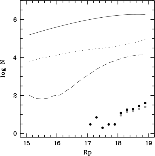
Figure 1: Differential number counts of objects with red Gaia/ WISE colours in the range covered by $z>4.5$ quasars. Solid line: all objects satisfying criteria specified in Sect. 2.1. Dotted line: sample after removing objects with parallaxes or proper motions identifying them as Milky Way stars. Dashed line: the sample after removing objects without parallax and proper motion measurements. Symbols: known high-redshift quasars before (black) and after (grey) removing those excluded by the dashed-line rule.

2 Data

In this section, we describe how we select candidates for high-redshift quasars in the Southern hemisphere from survey catalogues using information on spectral energy distributions (SEDs) and on apparent motions that can be seen for nearby stars. Quasars at high redshift are characterised by three features in their SEDs that help differentiate them from other objects:

1. At wavelengths shorter than the Ly $\alpha$ emission line the intrinsic quasar light is strongly attenuated by intergalactic absorption, creating a red colour between passbands located on either side of the line (e.g. at $z\approx 4.8$ the Ly $\alpha$ line appears at 700 nm).

2. At wavelengths just longer than the Ly $\alpha$ emission line the typical quasar continuum is bluer than most other objects.

3. Relative to stars, the optical-minus-mid-infrared colours of high-redshift quasars are redder. Colours such as $z-W1$ capture mostly the blue Rayleigh-Jeans tail in the spectra of cool stars, while the accretion disk continuum in quasar SEDs comprises black-body contributions across a range in temperature, and given the high redshift we do not see their tails.

Following the example of Wang et al. (2016), we use optical as well as mid-infrared photometry to select quasar candidates. Mid-infrared photometry from WISE has been immensely helpful for selecting quasars with high completeness across the whole range of redshifts from $z\approx 0$ to beyond $z\approx 4$ (e.g. Wu et al., 2012; Pâris et al., 2018). It is just at redshifts $z>4$ that the contamination by cool stars has traditionally been a challenge, which is here addressed with data from Gaia.

2.1 Parallax and proper motion information from Gaia

The Data Release 2 (DR2) of the Gaia mission (Gaia Collaboration et al., 2018) is the first and currently only release with parallax and proper motion measurements for objects as faint as we are targeting in this work. The release also contains photometry in two very broad passbands that cover roughly the wavelength range from 330 to 660 nm ($B_{p}$) and 630 to 1000 nm ($R_{p}$), respectively.

How useful parallaxes are for differentiating Galactic and extragalactic sources depends on the colours of the selected sources, hence it is not useful to consider a random subsample of Gaia sources. Instead we consult the sample of 795 quasars at $z>4.5$ collated by Wang et al. (2016) to learn what range of Gaia/ WISE colours they occupy and to quantify how much Gaia helps to reduce the contamination of candidate samples for high-z quasars specifically. The vast majority of known quasars at $z>4.5$ are fainter than 19 mag in SDSS $i$/$z$ bands. Some are too faint to be detected by Gaia, and at the highest redshifts we expect that their dominant flux is redshifted beyond the $R_{p}$ passband. However, the 111 brightest objects in the Wang et al. (2016) compilation, with either $i_{\rm AB}<19.2$ or $z_{\rm AB}<18.8$, all have a counterpart in Gaia DR2. Six of those 111 have $G$ band but no $B_{p}$ and $R_{p}$ photometry, while only one of them is bright enough to be missing from our later selection due to this issue.

At this point, we use only simple colour selections, as the Gaia argument does not depend on details. The detailed colour selection for this first candidate list among our works on high-redshift quasars will only be finalised in Sect. 2.4. Wang et al. (2016) show that $z>4.5$ quasars cover the interval $W1-W2=[0,2]$, although their own search is constrained to $W1-W2>0.5$ to avoid the dramatic stellar contamination below this threshold; this argument is based both on empirically found quasars as well as on the colour tracks of simulated quasars. They use further cuts, such as red colours in $z_{\rm SDSS}-W1$, for their candidates, and here we like to replace the SDSS filters with Gaia photometry as the latter is available for the whole sky. Using dereddened colours (see Sect. 2.4 for details), we find that the selection $(B_{p}-R_{p})_{0}>1.8$, $(R_{p}-W1)_{0}>2$, $W1-W2>0$ retains all of their $z>4.5$ quasars at $R_{p}<19$ except for one at $R_{p}=18.99$. We further select objects at galactic latitude $|b|>20\degr$ to avoid the denser star fields of the Galaxy, leaving a sky area of $\sim 26\,000$ deg². In Fig. 1 we show the number counts of Gaia objects satisfying these criteria: the solid line represents the whole sample of objects satisfying the simple colour cuts above. At $R_{p}<18$, the full object sample contains $\sim 11$ million objects. The symbols represent quasars from MILLIQUAS v6.2 (Flesch, 2015), which at $R_{p}<18$ contains only 18 objects. Down to $R_{p}<19$, the numbers are 135 known quasars out of $\sim 20$ million objects in total.

We then remove objects with parallaxes or proper motions suggestive of Milky Way stars from this sample. At $R_{p}\la 18$, Gaia measures parallaxes with an error of $\sim 0.35$ milli-arcsec (mas) per year and proper motions with $\sim 0.5$ milli-arcsec (mas) per year in each coordinate axis. We thus choose to remove objects with a parallax of $>1$ mas per year and those with a proper motion of $\sqrt{{\rm pmra}^{2}+{\rm pmdec}^{2}}>\sqrt{2}$ mas per year. At $R_{p}<18$ this leaves $\sim$300,000 objects, whose number counts are shown as the dotted line. Hence, 97.3% of the initial sample have been removed based on positive evidence of star-like motions.

An optional, more stringent, step is to remove objects for which Gaia does not provide any parallax and proper motion measurements in DR2. This will produce a purer candidate list at the risk of introducing incompleteness. Adding this criterion shrinks the sample to only 21,923 objects at $R_{p}<18$ or 1 part in $\sim$500 of the original sample (dashed line in Fig. 1).

Using MILLIQUAS we estimate the incompleteness caused by applying cuts based on Gaia’s motion data, which is appropriate since the previously known quasars were found before Gaia data had become available, and used only colour criteria. At $R_{p}<18$ all 18 known quasars pass the motion cuts, but incompleteness sets in when going fainter, mostly because the errors on Gaia’s proper motion measurements increase significantly. Fig. 1 shows the known quasars passing the stringent motion-based cuts as grey symbols. At $R_{p}=[18,18.5]$ and $R_{p}=[18.5,19]$, the cuts lose $\sim$20% and $\sim$33% of the quasars, respectively. Of course, a more complete and efficient selection function could take motion errors into account on a per-object basis, which will be advisable when exploring fainter magnitudes, but as this is beyond the scope of this paper, we continue with the selection motivated above.

We summarise here that, before further colour selections are made, we reduced a list of $\sim$11 million objects at $R_{p}=[15,18]$ to $\sim$22,000 objects based on Gaia’s motion data. This list covers 26,000 deg² of sky, in which 18 high-redshift quasars had been listed in MILLIQUAS, although not the whole area had been searched systematically before SkyMapper data became available.

2.2 The SkyMapper Southern Survey

SkyMapper is a 1.3m-telescope at Siding Spring Observatory near Coonabarabran in New South Wales, Australia (Keller et al., 2007). It started a digital survey of the whole Southern hemisphere in 2014. The survey provides photometric data in six optical passbands. The only two SkyMapper bands we use in this work are the $i$ and $z$ bands, which have transmission curves that are similar to those of the eponymous SDSS filters. Differences in width and central wavelength are below 30 nm, and the SkyMapper passbands can be approximated by $(\lambda_{\rm cen}/{\rm fwhm})$ of (779/140) and (916/84) for $i$ and $z$, respectively.

When the first release of the SkyMapper Southern Survey (DR1; Wolf et al., 2018a) became available in 2017, we started our search for high-redshift quasars, finding two of the objects reported here. When Gaia DR2 was released in April 2018, we accelerated our efforts, which led within a couple of days to the discovery of the quasar with the highest UV-optical luminosity known to date (Wolf et al., 2018b) and further objects.

Recently, the second release (DR2) became available to Australian astronomers (Onken et al., 2019). It mostly supersedes the first in sky coverage, depth and calibration quality, but also drops some of the older images by applying stricter quality limits. While DR1 was complete to $i\approx 18.2$, DR2 goes to $i\approx 19.5$ mag on nearly 90% of the Southern hemisphere. DR2 includes many more images, but its production was more selective in terms of image quality. As a result, 1% of the sky area in DR1 has no $i$ or $z$ photometry in DR2. We note that two of the quasars we found before DR2 are in this lost area. One lacks photometry in the $z$ band, and the other is not in the DR2 catalogue at all.

Although our work was started with DR1, we choose to report our results based on data from the superior DR2. For the two objects without $z$ band photometry in DR2, we borrow their photometry from DR1 for the purpose of estimating their luminosity. Calibration differences between the two releases are small enough, such that if their $i$/$z$ magnitudes had been available in DR2, they would still have been selected as candidates. We expect the next release from SkyMapper to contain twice as many Main-Survey images and include those two objects again.

2.3 Sample selection and quality flags

The master table in the SkyMapper data release has cross-matches to Gaia and AllWISE. We consider SkyMapper objects that have a Gaia match within $2^{\prime\prime}$ (to accommodate centroid shifts when SkyMapper blends sources that are close together) as well as a WISE match within $4^{\prime\prime}$ distance. We also require photometric errors in WISE of ${\rm W1sigmpro}<0.1$ and ${\rm W2sigmpro}<0.2$, while we make no such requirements for Gaia and SkyMapper since cuts in these bands are less critical when $R_{p}\la 18$. We find that $\sim$50% of Gaia sources at $|b|>20$ deg and $R_{p}<18$ have SkyMapper counterparts, driven by the survey footprint: SkyMapper covers nearly exactly the Southern hemisphere while Gaia is all-sky. Requiring a counterpart from the AllWISE all-sky table reduces the sample by $\sim 5$%; the lost objects are most likely stars, which have bluer optical/mid-infrared colours than high-redshift quasars and thus the latter would be bright enough to be all retained by this rule.

We exclude two regions centred on the two Magellanic Clouds with an area of $\sim 190$ deg². This leaves an effective search area of approx. 12,500 deg², as shown in Fig. 3. Finally, we remove 0.05% of objects, whose SkyMapper DR2 flags indicate that their photometry is not reliable (${\rm flags}>3$). SkyMapper flags up to value 255 come from Source Extractor (Bertin & Arnouts, 1996), but we also use bespoke flags with higher values to indicate sources that are likely affected by either scattered light from nearby bright stars (with $i<6$ mag or $z<5$ mag), or possibly by uncorrected cosmic rays as indicated by higher light concentration than is allowed for a point source (for details see Onken et al., 2019).

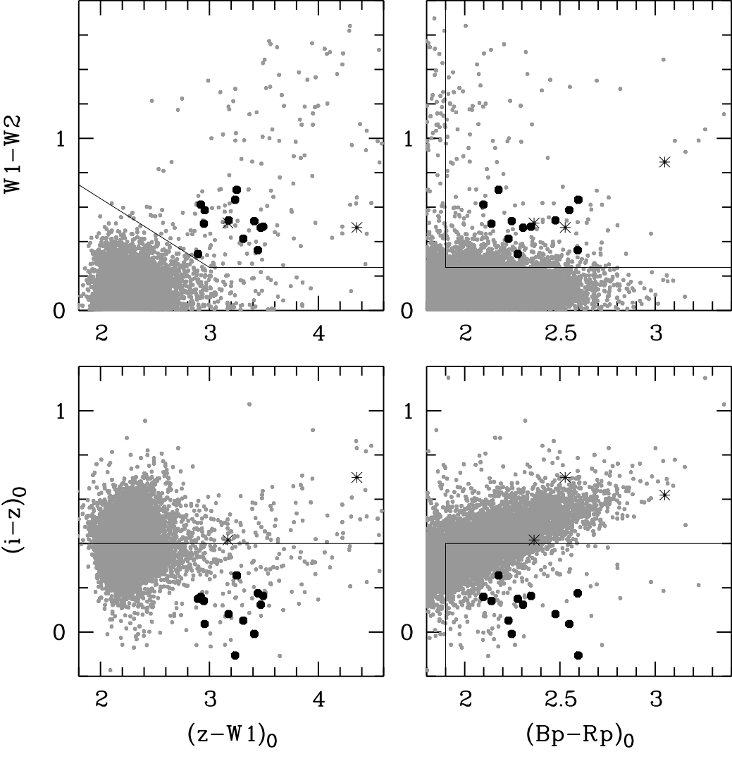
Figure 2: Colour-colour diagrams of objects with red Gaia/ WISE colours and magnitude $R_{p}=[15,18.2]$ after applying motion cuts. Small grey symbols are all objects, round black symbols are known $z\ga 4.5$ quasars and asterisks are known Carbon stars. Lines indicate the selection cuts.

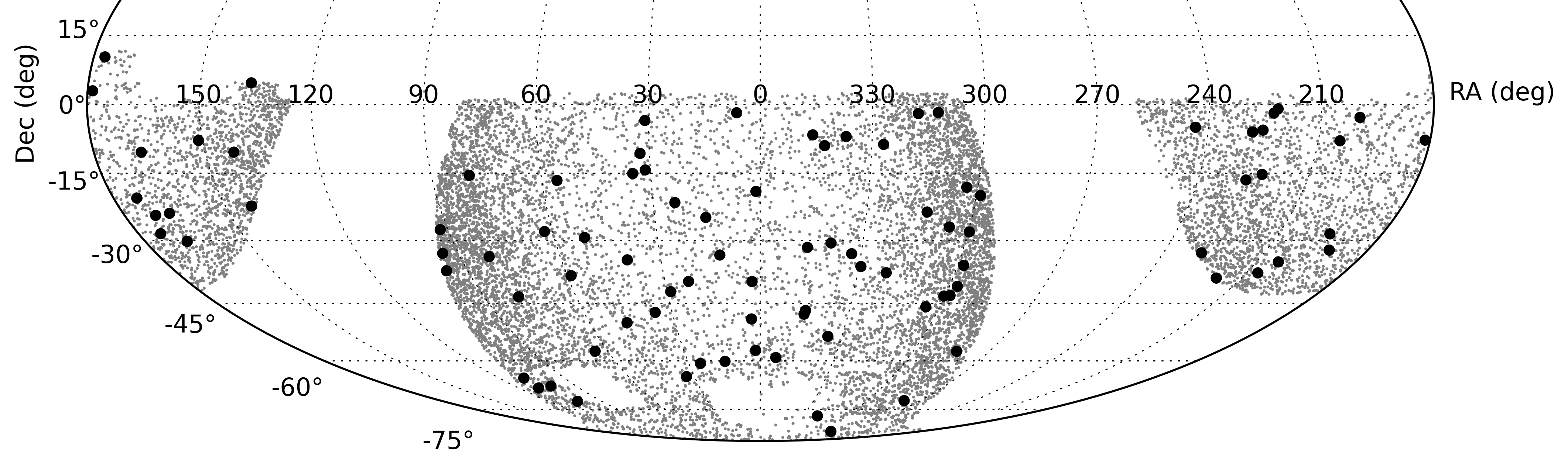
Figure 3: Sky map of objects with red Gaia/ WISE colours in the magnitude range $R_{p}=[15,18.2]$ after applying motion cuts. Small grey symbols are all 13 362 objects from $\sim$12 500 deg² of effective search area, and large black symbols show our 92 final candidates selected by the cuts illustrated in Fig. 2.

2.4 Colour selection

We explore colour criteria for selecting high-redshift candidates using Gaia $B_{p}$ and $R_{p}$, SkyMapper $i$ and $z$, and WISE W1 and W2 bands. We start with a sample of objects that is expected to contain nearly all $z=[4.5,5.2]$ quasars with typical SEDs, using dereddened colour cuts of $(B_{p}-R_{p})_{0}>1.8$, $(R_{p}-W1)_{0}>2$ and $W1-W2>0$, as already motivated and chosen in Sect. 2.1.

We corrected SkyMapper and Gaia magnitudes for interstellar extinction using the reddening maps by Schlegel, Finkbeiner, & Davis (1998, hereafter SFD), while leaving WISE data unchanged given the long wavelength. We adopt reddening coefficients from Wolf et al. (2018a), whose $R_{i}=1.582$ and $R_{z}=1.2$ are used with $A=R\times E(B-V)_{\rm SFD}$, and for Gaia from Casagrande & VandenBerg (2018), whose $R_{B_{p}}=3.374$ and $R_{R_{p}}=2.035$ are used with $A=R\times 0.86E(B-V)_{\rm SFD}$.

We search a magnitude range of $R_{p}=[15,18.2]$, given that the brightest known objects at $z>4$ have $R_{p}\approx 17$, and that we are interested in the brightest possible quasars in this first step of our work (in future work, we will reach deeper magnitudes as more telescope time for follow-up becomes available). Finally, we apply the stringent motion cuts from Section 2.1. The resulting 13 362 objects are shown in colour-colour diagrams in Fig. 2.

The black round symbols mark twelve high-z quasars in our sample that were already known when we started this work. Four of these are at $z\approx 4.4$, just outside the notional redshift interval we are aiming for, but equally relevant. Three further objects with known spectra are Carbon stars, marked by asterisk symbols. The latter can have extremely red optical/mid-infrared colours, and some are known at $(z-W1)_{0}=[5,8]$, beyond our diagrams.

In the next step, we deselect the dense clump of Milky Way stars and define a candidate list for spectroscopic follow-up using further and tighter colour cuts. We aim for discovering our first batch of ultra-luminous high-redshift quasars and won’t yet apply Bayesian selection approaches, but use conservative cuts aimed for purity; the spectroscopic follow-up of this candidate list is done with observations of one candidate at a time. In the near future, we will be able to follow up vastly larger candidate lists as ancillary science targets embedded in the Taipan Survey (da Cunha et al., 2017); then we will aim for a complete sample by penetrating the stellar locus. For now, however, we define candidates using the following criteria:

$$(B_{p}-R_{p})_{0}>1.9~{}~{}{\rm,}~{}~{}W1-W2>0.25~{}~{}{\rm,}~{}~{}(i-z)_{0}<0.4$$ (1)

$$~{}~{}{\rm and}~{}~{}W1-W2>0.25+0.4\times(3-(z-W1)_{0})$$ (2)

These criteria selected 92 candidates with $R_{p}<18.2$ for spectroscopic follow-up. None of the known $z>4.5$ quasars would be missed by these criteria, even if we pushed as faint as $R_{p}=18.8$, except for the object without $R_{p}$ data. Only at $R_{p}>18.8$ would we miss objects, presumably due to colour scatter from higher photometric errors. Results are discussed in Tab. 1 and Sect. 3. Without the motion cuts another 3 478 candidates would have been selected, so the Gaia data allowed us to compress the candidate list by a factor of $\sim$40 even in this part of colour space that is away from the main stellar locus.

Table 1: High-redshift quasars in our candidate sample. Four of the sources are radio-loud and detected in the radio survey NVSS; one of them (J052506.17-334305.6) is also detected in SUMSS. Errors on $R_{p}$, $z_{\rm PSF}$ and W1 range from 0.01 to 0.03 mag, well below the intrinsic variability of quasars. The average error on W1$-$W2 is 0.05 mag, but ranges from 0.04 to 0.09 mag. We only quote errors for the $H$ band, which are less homogenous.

object	redshift	$R_{p}$	$z_{\rm PSF}$	$H$	W1	W1$-$W2	$M_{145}$	$M_{300}$	Comments
		(Vega)	(AB)	(Vega)	(Vega)	(Vega)	(AB)	(AB)
Quasars observed in this work
J000500.21-185715.3	4.56	18.050	18.33	$16.72\pm 0.06$	15.43	0.35	$-27.85$	$-28.14$
J000736.56-570151.8	4.25	16.989	17.21	$15.73\pm 0.03$	14.72	0.55	$-28.88$	$-29.03$
J001225.00-484829.8	4.59	17.541	17.59	$16.01\pm 0.02$	14.46	0.51	$-28.33$	$-28.86$	$z_{\rm PSF}$ only in SMSS DR1
J013539.28-212628.2	4.94	17.886	17.73	$15.84\pm 0.15$	14.14	0.70	$-28.59$	$-29.27$	NVSS $25.3\pm 0.9$ mJy
J022306.73-470902.5	4.95	18.079	18.04	$15.94\pm 0.01$	14.55	0.59	$-28.34$	$-29.06$
J040914.87-275632.9	4.45	17.552	17.86	$16.20\pm 0.03$	14.68	0.49	$-28.32$	$-28.64$	Schindler et al. (2019b)
J051508.92-431853.7	4.61	18.064	18.06	$16.25\pm 0.04$	14.60	0.40	$-28.03$	$-28.64$
J065522.86-721400.3	4.34	18.106	18.40	$16.65\pm 0.07$	14.87	0.39	$-27.84$	$-28.19$
J072011.68-675631.7	4.70	17.966	17.88	$16.22\pm 0.04$	14.29	0.53	$-28.33$	$-28.77$
J093032.57-221207.7	4.86	18.045	18.06	$16.49\pm 0.05$	15.43	0.55	$-28.37$	$-28.50$
J110848.48-102207.2	4.45	17.989	18.21	$16.48\pm 0.03$	15.16	0.50	$-27.95$	$-28.37$	Schindler et al. (2019b)
J111054.69-301129.9	4.80	17.334	17.27	$15.55\pm 0.04$	14.27	0.52	$-29.05$	$-29.41$	Yang et al. (2018b)
J151204.27-055508.4	4.00	18.188	18.30	$16.45\pm 0.02$	14.91	0.38	$-27.40$	$-28.22$
J151443.82-325024.8	4.81	17.758	17.83	$15.82\pm 0.03$	13.99	0.67	$-28.96$	$-29.34$
J211920.80-772252.9	4.52	17.399	17.56	$16.03\pm 0.04$	14.77	0.50	$-28.58$	$-28.87$	only in SMSS DR1
J215728.21-360215.1	4.75	17.136	17.10	$14.80\pm 0.03$	13.10	0.51	$-29.30$	$-30.15$	Wolf et al. (2018b)
J221111.55-330245.8	4.64	18.099	18.16	$15.94\pm 0.01$	13.85	0.61	$-27.99$	$-28.98$
J222759.64-065524.0	4.50	17.908	18.02	$16.44\pm 0.02$	14.76	0.42	$-28.30$	$-28.42$
J230349.19-063343.0	4.68	18.044	17.96	$15.96\pm 0.02$	14.55	0.47	$-28.13$	$-28.97$
J230429.88-313426.9	4.84	17.653	17.79	$16.13\pm 0.01$	14.62	0.61	$-28.61$	$-28.85$
J233505.85-590103.1	4.50	17.267	17.45	$15.92\pm 0.01$	14.43	0.45	$-28.79$	$-28.92$
Quasars known previously
J002526.83-014532.5	5.07	17.990	18.07	$16.26\pm 0.03$	14.80	0.64	$-28.41$	$-28.83$
J030722.86-494548.3	4.78	17.371	17.36	$15.69\pm 0.01$	14.38	0.58	$-28.96$	$-29.25$
J032444.28-291821.0	4.62	17.607	17.76	$16.29\pm 0.01$	14.84	0.33	$-28.43$	$-28.60$	NVSS $236.5\pm 7.1$ mJy
J035504.86-381142.5	4.58	17.232	17.42	$15.59\pm 0.10$	13.94	0.48	$-28.75$	$-29.27$
J041950.93-571612.9	4.46	18.132	18.44	$16.67\pm 0.04$	15.01	0.52	$-27.80$	$-28.16$
J052506.17-334305.6	4.42	18.011	18.18	$16.31\pm 0.04$	14.90	0.70	$-27.80$	$-28.51$	NVSS $188.3\pm 5.7$ mJy
J071431.39-645510.6	4.44	17.741	17.91	$16.33\pm 0.04$	14.85	0.50	$-28.27$	$-28.53$	gravitationally lensed
J090527.39+044342.3	4.40	17.812	18.24	$16.27\pm 0.03$	14.70	0.49	$-27.84$	$-28.55$	blended in SMSS DR2 table
J120523.14-074232.6	4.69	17.853	17.92	$16.22\pm 0.03$	14.70	0.52	$-28.37$	$-28.70$
J130031.13-282931.0	4.71	18.022	18.05	$16.35\pm 0.04$	14.51	0.35	$-28.23$	$-28.62$
J145147.04-151220.1	4.76	17.016	17.10	$15.35\pm 0.01$	13.69	0.42	$-29.29$	$-29.63$	NVSS $28.5\pm 1.0$ mJy
J211105.60-015604.1	4.85	18.007	17.96	$16.39\pm 0.03$	15.02	0.61	$-28.48$	$-28.61$
J214725.70-083834.5	4.59	17.795	17.97	$16.38\pm 0.04$	15.00	0.61	$-28.22$	$-28.51$
J223953.66-055220.0	4.56		17.71	$15.90\pm 0.02$	14.09	0.47	$-28.46$	$-28.98$	no Gaia $R_{p}$ measurement

2.5 Spectroscopy at the ANU 2.3m-telescope

We took spectra of the candidates with the Wide Field Spectrograph (WiFeS; Dopita et al., 2010) on the ANU 2.3m-telescope at Siding Spring Observatory. We used 18 nights, most of which were useful (2018 April 29, Sep 16 to 18, Dec 4, 5; 2019 March 11 to 13, 30, April 1, June 30, July 1 to 5, Aug 29). Two quasars were identified already with earlier observations on 2017 December 21 during a pilot search that had not yet benefited from Gaia data.

We used the WiFeS B3000 and R3000 gratings in the blue and red arm, which between them cover the wavelength range from 3600 Å to 9800 Å at a resolution of $R=3000$. Exposure times ranged from 600 sec to 1 800 sec, and observing conditions varied significantly in terms of cloud cover and seeing.

The data were reduced using the Python-based pipeline PyWiFeS (Childress et al., 2014). PyWiFeS calibrates the raw data with bias, arc, wire, internal-flat and sky-flat frames, and performs flux calibration and telluric correction with standard star spectra. Flux densities were calibrated using several standard stars throughout the year, which are usually observed on the same night. We then extract spectra from the calibrated 3D cube using a bespoke algorithm for fitting and subtracting the sky background after masking sources in a white-light stack of the 3D cube.

We obtained spectra with for all candidates except the objects reported in the literature. Reduced spectra were visualised with the MARZ software (Hinton et al., 2016) and quasar templates were overplotted to aid the redshift determination. We estimate redshifts from broad Si iv and C iv lines where available, and consider the blue edge of the Ly $\alpha$ line when necessary. We estimate that redshift uncertainties range from 0.01 to $\sim$0.05 for the weak-lined objects. Despite good signal, four of the 92 candidates from our sample remain currently unclassified. Their spectra are unlike anything we have seen before, and we deem them unlikely to be high-redshift quasars.

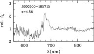
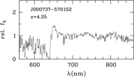
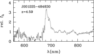
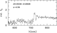
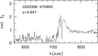
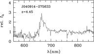
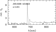
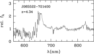
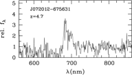
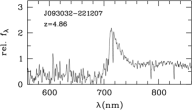
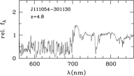
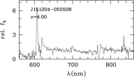
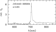
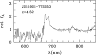
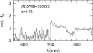
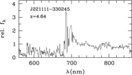
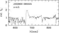
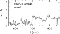
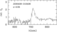
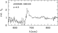
Figure 4: Gallery of 21 quasar spectra with $z\geq 4$ observed by us. The two quasars with weak emission lines have clearly visible Lyman forests in the 2D spectra. Example spectra from the 24 red or unusual quasars at lower redshift are shown in Fig. 6.

Figure 5: Ultra-luminous high-redshift quasars with $R_{p}<18.2$, known before this work (grey) and identified in this work (black, see Table 1). Our sample improves especially in the regime of high bolometric luminosity, for which $M_{300}$ is a useful proxy.

3 Results

3.1 High-redshift quasars among the candidates

The spectroscopy revealed 21 ultra-luminous quasars at $z\geq 4$ (see Fig. 4), of which 18 are newly identified. The most luminous object among the new 18 was already reported in Wolf et al. (2018b). Three more objects in our sample were independently observed by other teams and published in the literature only after our observations were done: Yang et al. (2018b) revealed a $z=4.8$ quasar and Schindler et al. (2019b) found two more quasars at $z=4.45$. Three of the newly identified objects are at slightly lower redshifts of $z=4$, $z=4.25$ and $z=4.34$, while the others are at $z\geq 4.5$ as expected.

In the bottom part of Table 1 we list 13 further high-redshift quasars in our sample, and one outside our sample, that were known already when our observations commenced: ten of them are in the target redshift window of $z=[4.5,5.2]$ and four more at slightly lower redshifts. Altogether then, 34 objects out of 92 candidates with good spectra are quasars at high redshifts of $z\geq 4$.

As a result of this work, we have lifted the number of known bright ($R_{p}<18.2$) $z\geq 4.5$ quasars in the Southern hemisphere from ten objects prior to our observations to 26 now.

We derive luminosities in two restframe bands, $M_{145}$ centred at 145 nm and $M_{300}$ at 300 nm, and show the impact of our work on the luminosity-redshift space of known quasars in Fig. 5. For previously discovered quasars, authors most often listed $M_{145}$ as it is constrained by the $i$ and $z$ passbands in which the optical discovery is made, and usually also covered in the spectrum, so it can be determined while avoiding influence from the broad emission lines. Also, $M_{145}$ is the best available proxy for the ionising flux from the quasar. Measuring $M_{300}$, in contrast, requires $HK$ photometry, which has previously been available only for the most extreme objects that were bright enough to be detected by the 2 Micron All-Sky Survey (2MASS; Skrutskie et al., 2006). $M_{300}$ is a better predictor of the bolometric luminosity of quasars as it is closer to the peak in their spectral energy distribution. Now, the much deeper VISTA Hemisphere Survey (VHS) and the VIKING survey (Edge et al., 2013) are available, at least in the Southern hemisphere, and provide very precise photometry for most quasars in our sample.

We estimate $M_{145}$ first for all objects in Table 1 with a simple linear interpolation of the SkyMapper $i$ and $z$ band photometry. For the subset of objects with spectra from the 2.3m-telescope, we also measure $M_{145}$ from the spectra after normalising them to the photometry. As we find no differences larger than $\pm 0.05$ mag, we report the simpler measure of $M_{145}$ that is available for all objects consistently. We do not report errors as they are smaller than the intrinsic long-term stochastic variability of quasars.

We measure $M_{300}$ in the best case from $H,K_{s}$ photometry in the VHS; these objects have $H$ band errors up to $0.03$. For a few objects, VHS currently has $J,K_{s}$ photometry but no $H$ band, and for these we estimate $H$ magnitudes from $J,K_{s}$ photometry. For most objects, we have all three near-infrared magnitudes, $J,H,K_{s}$, and for those we find that $(H-K_{s})/(J-K_{s})=0.41\pm 0.028$. We apply this tight relation to derive $H(J,K_{s})$ and combine the measurement and relation errors; the resulting $H$ band errors range from $0.03$ to $0.07$. Five objects have no VHS coverage but we find three of them in VIKING (J032444-291821, J221111-330245 and J230429-313426), one in UKIDSS (J090527+044342), and for the final one (J013539-212628) we resort to 2MASS photometry, which has a larger $H$ band error of $0.15$ mag. However, we stress that all these errors are smaller than the intrinsic long-term variability of quasars.

3.2 Radio detections

None of the listed objects is detected in the 1.4 GHz VLA survey ”Faint Images of the Radio Sky at Twenty-Centimeters” (FIRST; Becker et al., 1995), mostly due to its mostly Northern sky coverage. The 1.4 GHz NRAO-VLA Sky Survey (NVSS; Condon et al., 1998) covers the sky at $\delta>-40\degr$ with a flux limit of 2.5 mJy; it contains four of the quasars; one of these, J052506.17-334305.6, is also detected by the 843 MHz Sydney University Molonglo Southern Survey (SUMSS; Bock et al., 1999), which covers the polar half of the Southern hemisphere at $\delta<-30\degr$ with a limit of 5 mJy. Its fluxes of $183.8\pm 5.9$ at 843 MHz and $188.3\pm 5.7$ at 1.4 GHz suggest that it is a flat-spectrum radio quasar (FSRQ; Urry & Padovani, 1995).

We use the radio-to-optical ratio $R=f_{\nu,\rm 6cm}/f_{\nu,B}$ defined by Kellermann et al. (1989) to label objects as radio-loud ($R>10$) or radio-quiet ($R<1$); in that work the ratio is based on the flux density at 6 cm and 440 nm wavelength for a sample with average redshift of $\sim 0.5$, but for our objects these bands are redshifted on average ($z=4.75$) to $\sim 23$ cm, which is approximately the NVSS wavelength, and 1700 nm, which is in the NIR $H$ band. A sensitivity limit of $f<2.5$ mJy in the NVSS corresponds to $R<10$ for $H=16.6$, the typical magnitude of the faintest sources in this work, and $R<2$ for the $H=14.8$ of the brightest source.

The four sources detected by NVSS and SUMSS range from $R\approx 40$ to $R\approx 300$ and are thus clearly radio-loud. Of these four, one is newly discovered and three have been known as quasars before. This is consistent with the fact that the fraction of radio-loud quasars is generally small, while known quasars in the Southern hemisphere have previously often been discovered by optical follow-up of radio source catalogues. All except one of the newly discovered quasars are thus radio-quiet.

3.3 Gravitationally lensed quasars?

Gravitationally lensed quasars are intrinsically very rare, but their fraction is higher among quasars of brighter apparent magnitude, as their brightness is boosted by the lensing. When quasars are lensed, they show multiple magnified images and hence their luminosity is overestimated. We thus look for signs of multiplicity among the objects in the Gaia catalogue, which is known to be incomplete at separations of $<2$ arcsec. We find just one object that has a Gaia neighbour within 5 arcsec, J090527.39+044342.3. There, we actually see two objects in the SkyMapper image coincident with two Gaia sources separated by 4 arcsec. The catalogued SkyMapper source is a blend of the two objects, with the centroid location close to the brighter of the two. The SDSS DR14 has separate photometry for the two sources and shows the fainter source to have colours that are different from the first and typical for a star. Hence, these are not expected to be two images of one object. The SkyMapper PSF magnitudes are 0.2 mag fainter than the SDSS measurements of the (brighter) quasar source; this is either a consequence of long-term variability, or the blending causes the SkyMapper PSF magnitude and the luminosity to be underestimated here.

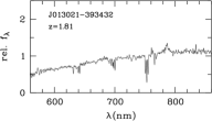
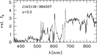
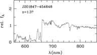
Figure 6: Gallery of three lower-redshift quasar spectra. Left: a generally red continuum. Centre: a BALQSO. Right: an OFeLoBAL QSO.

3.4 Contaminants in candidate sample

Most contaminants in our candidate sample turn out to be cool stars and include a few carbon stars and long-period variables. But we also identify 24 quasars at lower redshift. Typical quasars at those lower redshifts are firmly excluded by our selection cuts, and the spectra reveal that these quasars are unusual. They fall into three categories (see Fig. 6 for example spectra):

1. Five quasars at $z=0.5$ to $z=2$ have atypically red continua; Richards et al. (2003) found that 6% of quasars in a large SDSS sample fall into this category, which would be missed by surveys for quasars with typical, blue, colours.

2. Three quasars at $z\approx 2.6$ to $3.3$ have strong broad absorption lines (BALQSOs; Weymann et al., 1991; Scaringi et al., 2009), which render the emission lines nearly invisible. They are not easily separated from the other objects without resorting to spectra. Richards et al. (2003) also find that BALs are more common among red quasars.

3. 16 objects have extremely wide absorption troughs at nearly full depth, such that it is very challenging to determine any redshift at all. Objects with qualitatively similar spectra have been found in the past and typed as OFeLoBALQSOs (Overlapping Iron Low-Ionisation Broad-Absorption line QSOs) by Hall et al. (2002) and Zhang et al. (2015). Their spectra are believed to be nearly fully absorbed bluewards of the Mg ii line, which suggest a rough redshift based on the assumption that the unabsorbed continuum starts around 280 nm wavelength. If this is true, the objects we found would all reside at redshift $z\approx 1$ to $2$. This category of objects will be discussed in a separate publication.

The number of lower-$z$ quasars with unusual SEDs is roughly as large as the number of true high-$z$ quasars and may come as a surprise when compared to earlier surveys. They also reach $\sim$1 mag brighter in $R_{p}$ than the $z>4.5$ quasars. It seems clear, how the lower-$z$ OFeLoBALQSOs are confused with $z>4.5$ quasars: the strong suppression bluewards of the Mg ii line simply mimics the effect of Lyman forest. But why are they more common than in previous searches? We believe, this is because we target high-$z$ quasars of such high and rare luminosity that we run out of objects, while the interlopers appear still with their natural abundance.

We note that nearly all the $z<2.5$ quasars, whether those with generally red continua or the OFeLoBALQSOs with extreme absorption bluewards of the Mg ii line, have WISE colours of $W1-W2\approx[1,1.5]$, which are typical for quasars at $z<2$ (see Fig. 7). In contrast, all of the high-redshift ($z\geq 4$) quasars in this work have $W1-W2=[0.3,0.75]$ (see Fig. 7), with a mean colour of $0.52$; the RMS scatter of $0.11$ appears to be mostly intrinsic, as the average error on the W1$-$W2 colour is $0.053$. The conclusion is, however, that we could distinguish low-redshift interlopers from high-redshift objects using appropriate ranges in $W1-W2$ colour. We note that the high-redshift quasars reported in Wang et al. (2016) include objects with $W1-W2$ colours as red as $\sim$1.7 despite moderate errors on the WISE photometry, although these are all fainter than our search regime. Either the errors of their WISE photometry is underestimated or high-redshift quasars with red mid-infrared colours are intrinsically rare at the highest luminosity studied here, so that none show up in our sample.

Figure 7: Confirmed quasars in our selected sample: at $z=[4,5]$ they have $W1-W2=[0.3,0.75]$, while lower-redshift quasars are redder. They are in our sample because of red continua, strong BAL features, or extreme absorption bluewards of the Mg ii line as in the case of OFeLoBAL QSOs.

4 Summary

We used data from SkyMapper DR1 and DR2, from Gaia DR2 and from AllWISE to search for quasar candidates at $z>4.5$ in the Southern hemisphere. We focus on the bright end of the quasar distribution, where true quasars are outnumbered by cool stars to the most extreme degree possible.

The role of Gaia DR2 is primarily to remove the vast majority of objects in the search space, which are cool stars in our own Milky Way that show noticeable parallax or proper motion. The Gaia data allow us to reduce the target density by a factor of $\sim$40 now and several hundred in the future.

In this paper, we focus on very likely quasars and suppress stellar contamination further with a colour-based selection. In an area of $\sim$12 500 deg², we find 92 high-redshift candidates with a brightness of $R_{p}<18.2$, among which were 13 already known high-redshift quasars. We take spectra of the others and identify 21 more quasars, three of which have been identified and published independently since our observations.

This new sample increases the number of Southern $z\geq 4.5$ quasars at $R_{p}<18.2$ from 10 to 26, and takes the number in the whole sky to 42. The new quasars are mostly in the luminosity range of $M_{145}\approx[-29,-28]$. At this point we refrain from investigating luminosity functions, because our search for more quasars will continue into more challenging parts of search space; those have been avoided in the past due to the abundance of cool stars that appear with similar colour to quasars and dramatically inflate the candidate samples. However, this area of search space is critical for assembling complete samples of quasars and will soon become accessible, owing to Gaia DR2 and because spectroscopic follow-up of many thousand targets at low sky density is becoming affordable with projects such as the Taipan Survey.

We also find among our candidates 24 lower-redshift quasars with unusual red spectra, most of which appear to be OFeLoBALQSOs. These are particularly prevalent in our sample relative to $z>4.5$ quasars, because we target a magnitude range where high-redshift quasars are truly rare, shifting the balance in favour of unusual low-$z$ objects. However, they can easily be distinguished using mid-infrared colours: while the rule $W1-W2<0.75$ retains all our high-redshift objects, it removes most low-redshift interlopers.

In the future, we will venture into the stellar locus with massive spectroscopic follow-up, and revisit also part of the Northern sky with this approach, taking advantage of the Gaia motion measurements. We will also go deeper and to redshifts $z>5$. Finally, we will pursue measurements of black-hole masses for our sample.

References

- Bañados et al. (2018) Bañados E. et al., 2018, Nature, 553, 473
- Becker et al. (1995) Becker, R. H., White, R. L., & Helfand, D. J. 1995, ApJ, 450, 559
- Bertin & Arnouts (1996) Bertin, E., Arnouts, S., 1996, A&AS, 117, 393
- Bock et al. (1999) Bock, D. C.-J., Large, M. I., & Sadler, E. M. 1999, AJ, 117, 1578
- Bromm & Loeb (2003) Bromm, V., & Loeb, A. 2003, ApJ, 596, 34
- Casagrande & VandenBerg (2018) Casagrande L., VandenBerg D. A., 2018, MNRAS, 479, L102
- Childress et al. (2014) Childress, M. J., Vogt, F. P. A., Nielsen, J., & Sharp, R. G. 2014, Ap&SS, 349, 617
- Condon et al. (1998) Condon, J. J., Cotton, W. D., Greisen, E. W., et al. 1998, AJ, 115, 1693
- da Cunha et al. (2017) da Cunha, E., Hopkins, A. M., Colless, M. et al. 2017, PASA, 34, e047
- Díaz et al. (2014) Díaz, C. G., Koyama, Y., Ryan-Weber, E. V. et al. 2014, MNRAS, 442, 946
- Dopita et al. (2010) Dopita, M., Rhee, J., Farage, C. et al. 2010, Ap&SS, 327, 245
- Dye et al. (2018) Dye S. et al., 2018, MNRAS, 473, 5113
- Edge et al. (2013) Edge A., Sutherland W., Kuijken K., Driver S., McMahon R., Eales S., Emerson J. P., 2013, ESO Messenger, 154, 32
- Fan et al. (2001) Fan X. et al., 2001, AJ, 121, 31
- Fitzpatrick (1999) Fitzpatrick, E. L., 1999, PASP, 111, 63
- Flesch (2015) Flesch E. W., 2015, PASA, 32, e010
- Gaia Collaboration et al. (2016) Gaia Collaboration, Prusti, T., de Bruijne, J. H. J. et al. 2016, A&A, 595, A1
- Gaia Collaboration et al. (2018) Gaia Collaboration, Brown, A. G. A., Vallenari, A. et al. 2018, arXiv:1804.09365
- Hall et al. (2002) Hall P. B., et al., 2002, ApJS, 141, 267
- Hinton et al. (2016) Hinton S. R., Davis T. M., Lidman C., Glazebrook K., Lewis G. F., 2016, Astronomy & Computing, 15, 61
- Jiang et al. (2016) Jiang L. et al., 2016, ApJ, 833, 222
- Keller et al. (2007) Keller, S. C., Schmidt, B. P., Bessell, M. S. et al. 2007, PASA, 24, 1
- Kellermann et al. (1989) Kellermann, K. I., Sramek, R., Schmidt, M., Shaffer, D. B., & Green, R. 1989, AJ, 98, 1195
- McMahon et al. (2013) McMahon, R. G., Banerji, M., Gonzalez, E. et al. 2013, The Messenger, 154, 35
- Mortlock et al. (2011) Mortlock D. J. et al., 2011, Natur, 474, 616
- Onken et al. (2019) Onken, C. A., Wolf, C., Shao, L., Luvaul, L. C. et al. 2019, PASA, 36, 33
- Pacucci, Volonteri & Ferrara (2015) Pacucci F., Volonteri M., Ferrara A., 2015, MNRAS, 452, 1922
- Pâris et al. (2018) Pâris I. et al., 2018, A&A, 613, A51
- Richards et al. (2003) Richards G. T., et al., 2003, AJ, 126, 1131
- Ross et al. (2015) Ross N. P., et al., 2015, MNRAS, 453, 3932
- Ryan-Weber et al. (2009) Ryan-Weber E. V., Pettini M., Madau P., Zych B. J., 2009, MNRAS, 395, 1476
- Scaringi et al. (2009) Scaringi S., Cottis C. E., Knigge C., Goad M. R., 2009, MNRAS, 399, 2231
- Schindler et al. (2018) Schindler J.-T. et al., 2018, ApJ, 863, 144
- Schindler et al. (2019a) Schindler J.-T. et al., 2019, ApJ, 871, 258
- Schindler et al. (2019b) Schindler J.-T. et al., 2019, arXiv e-prints, arXiv:1905.04069
- Schlegel, Finkbeiner, & Davis (1998) Schlegel D. J., Finkbeiner D. P., Davis M., 1998, ApJ, 500, 525
- Simcoe et al. (2011) Simcoe, R. A., Cooksey, K. L., Matejek, M. et al. 2011, ApJ, 743, 21
- Skrutskie et al. (2006) Skrutskie, M. F., Cutri, R. M., Stiening, R., Weinberg, M. D., et al. 2006, AJ, 131, 1163
- Urry & Padovani (1995) Urry, C. M., & Padovani, P. 1995, PASP, 107, 803
- Volonteri & Bellovary (2012) Volonteri M., Bellovary J., 2012, RPPh, 75, 124901
- Wang et al. (2016) Wang, F., Wu, X.-B., Fan, X. et al. 2016, ApJ, 819, 24
- Wang et al. (2017) Wang F. et al., 2017, ApJ, 839, 27
- Warren et al. (2007) Warren S. J. et al., 2007, MNRAS, 375, 213
- Weymann et al. (1991) Weymann R. J., Morris S. L., Foltz C. B., Hewett P. C., 1991, ApJ, 373, 23
- Wolf et al. (2018a) Wolf, C., Onken, C. A., Luvaul, L. C. et al. 2018, PASA, 35, 10 (doi: 10.4225/41/593620ad5b574)
- Wolf et al. (2018b) Wolf, C., Bian, F., Onken, C. A., Schmidt, B. P., Tisserand, P. et al. 2018, PASA, 35, 24
- Wright et al. (2010) Wright, E. L., Eisenhardt, P. R. M., Mainzer, A. K. et al. 2010, AJ, 140, 1868
- Wu et al. (2012) Wu X.-B., Hao G., Jia Z., Zhang Y., Peng N., 2012, AJ, 144, 49
- Wu et al. (2015) Wu, X.-B., Wang, F., Fan, X. et al. 2015, Nature, 518, 512
- Yang et al. (2017) Yang J. et al., 2017, AJ, 153, 184
- Yang et al. (2018b) Yang J. et al., 2019, ApJ, 871, 199
- Yang et al. (2019b) Yang J. et al., 2019, AJ, 157, 236
- York et al. (2000) York, D. G., Adelman, J., Anderson, J. E., Jr. et al. 2000, AJ, 120, 1579
- Zhang et al. (2015) Zhang S., et al., 2015, ApJ, 803, 58