Edge of chaos and avalanches in neural networks with heavy-tailed synaptic weight distribution
Abstract
We propose an analytically tractable neural connectivity model with power-law distributed synaptic strengths. When threshold neurons with biologically plausible number of incoming connections are considered, our model features a continuous transition to chaos and can reproduce biologically relevant low activity levels and scale-free avalanches, i.e. bursts of activity with power-law distributions of sizes and lifetimes. In contrast, the Gaussian counterpart exhibits a discontinuous transition to chaos and thus cannot be poised near the edge of chaos. We validate our predictions in simulations of networks of binary as well as leaky integrate-and-fire neurons. Our results suggest that heavy-tailed synaptic distribution may form a weakly informative sparse-connectivity prior that can be useful in biological and artificial adaptive systems.
Scale-free neuronal avalanches, commonly associated with criticality, have been observed in cortical networks in various settings, including cultured and acute slices from rat somatosensory cortex Beggs and Plenz (2003), eye-attached ex vivo preparation of turtle visual cortex Shew et al. (2015), visual cortex in anesthetized rats Fontenele et al. (2019), primary visual cortex in anesthetized monkeys Fontenele et al. (2019), and premotor, motor, and somatosensory cortex in awake monkeys Petermann et al. (2009). Criticality implies the existence of a continuous transition between two distinct collective phases. In the context of neuronal avalanches, most commonly studied transitions are between quiescent and active states Beggs and Plenz (2003); Haldeman and Beggs (2005); Kinouchi and Copelli (2006) or synchronuous and asynchronuous states di Santo et al. (2018); Fontenele et al. (2019). In addition to providing a plausible generating mechanism for the neuronal avalanches, the existence of a continuous transition would have important functional implications, as it has been shown that computation is most efficient around a critical point Kinouchi and Copelli (2006); Stoop and Gomez (2016); Munoz (2018), often associated with the edge of chaos Langton (1990); Bertschinger and Natschläger (2004); Legenstein and Maass (2007); Toyoizumi and Abbott (2011); Schuecker et al. (2018). However, the relation between neuronal avalanches, criticality, and edge of chaos is not fully understood Benayoun et al. (2010); Beggs and Timme (2012); Munoz (2018).
Different scenarios of the transition to chaos in randomly connected neural networks were extensively studied over the last years Sompolinsky et al. (1988); Molgedey et al. (1992); Amit and Brunel (1997); Brunel (2000); Rajan et al. (2010); Massar and Massar (2013); Stern et al. (2014); Aljadeff et al. (2015); Kadmon and Sompolinsky (2015); Wainrib and Galtier (2016); Crisanti and Sompolinsky (2018); Schuecker et al. (2018). According to the prevailing assumption rooted in the central limit theorem, the total synaptic input current of each neuron can be modeled as a Gaussian random variable (Gaussian assumption). Here we argue that the Gaussian assumption cannot account for some of the experimentally observed features of neuronal circuits.
In particular, the continuous nature of the phase transition observed in the conventional models is sensitive to theoretical assumptions that are not biologically grounded. Most works that study transition to chaos employ rate models with continuous non-thresholded activation functions, often of a sigmoidal shape Sompolinsky et al. (1988); Molgedey et al. (1992); Rajan et al. (2010); Stern et al. (2014); Aljadeff et al. (2015); Crisanti and Sompolinsky (2018); Schuecker et al. (2018). Sometimes thresholds are introduced, but often the analysis is restricted to the suprathreshold regime Kadmon and Sompolinsky (2015); Harish and Hansel (2015). But most neurons in the brain spike only when driven by strong enough excitatory synaptic input above a threshold Dayan and Abbott (2001); Häusser and Monsivais (2003); Gerstner et al. (2014). Thus, we model a self-sustained (autonomous) activity in a network of individually subthreshold neurons. Other models exhibiting continuous transition to chaos Bertschinger and Natschläger (2004) or neuronal avalanches Kinouchi and Copelli (2006); Millman et al. (2010) rely on extremely sparse ( connections per neuron) networks. However, many neurons in the vertebrate brain receive a large number of inputs from other cells () Dayan and Abbott (2005). We observed that the transition to chaos becomes discontinuous when densely connected subthreshold units are used in tandem with the Gaussian assumption (Fig. 3) Brunel (2000); Marshel et al. (2019). This discontinuous character of the transition makes it hard for the network to robustly exhibit the edge of chaos, low activity levels, or avalanches. Although a discontinuous transition can be smoothed by noise, leading again to critical behavior away from the edge of chaos if the noise level is appropriate Scarpetta et al. (2018), such noise-induced criticality requires extra fine-tuning. We explore instead the possibility that an autonomous network exhibits critical behavior at the edge of chaos.
To fix this issue, we draw on the experimental works reporting heavy-tailed distributions of synaptic weights in various areas of the brain Sayer et al. (1990); Feldmeyer et al. (1999); Song et al. (2005); Lefort et al. (2009); Ikegaya et al. (2012); Loewenstein et al. (2011). Multiple theoretical mechanisms have been suggested to realize such distributions, e.g. modified spike-timing-dependent plasticity (STDP) rule Gilson and Fukai (2011) or STDP combined with homeostatic plasticity Zheng et al. (2013). Notably, recent studies have suggested that experimentally observed activity-independent intrinsic spine dynamics can straightforwardly explain the heavy-tailed distributions of synaptic weights Yasumatsu et al. (2008); Nagaoka et al. (2016); Humble et al. (2019); Ishii et al. (2018); Okazaki et al. (2018).
Although extensively studied, the computational role of synaptic heavy tails is still not fully understood. A log-normal distribution is often assumed and the results are obtained by means of computer simulations Teramae et al. (2012); Ikegaya et al. (2012); Buzsáki and Mizuseki (2014); Teramae and Fukai (2014); Omura et al. (2015). Unfortunately, the log-normal distribution is not a stable distribution Feller (1971). Consequently, the corresponding distribution of the membrane potential depends in a nontrivial way on the details of the connectivity, including number of incoming connections. Moreover, if the number of incoming connections is scaled linearly with the number of neurons, the Gaussian assumption is recovered in the thermodynamic limit. This hinders theoretical approaches to study the effects of heavy-tails in these models. Therefore, a simple model that robustly predicts the effects of synaptic heavy tails is needed. We fill this gap by assuming random, power-law distributed synaptic weights.
Our aim is to inspect how the distribution of synaptic efficacies, modulated by the activation function, affects the transition to chaos and the associated avalanches. To this end, in our calculations we focus on the network effects and hence simplify the dynamics of individual neurons by considering the following discrete-time network dynamics
| (1) |
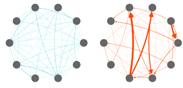
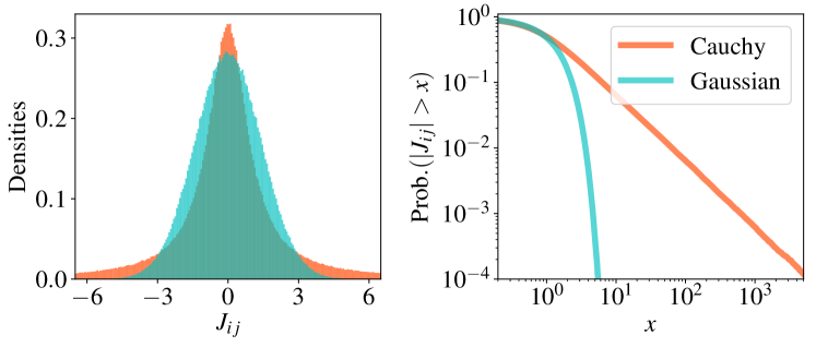
where is the activation function, assumed to be identical across the network, and is the connectivity matrix. The network is fully connected and the synaptic weights are independently drawn from the common Cauchy distribution (Fig. 1)
| (2) |
with the characteristic function
| (3) |
where defines the width of the distribution. We refer to the model prescribed by (1) and (2) as the Cauchy network.
Due to the generalized central limit theorem Feller (1971), in the thermodynamic limit of results obtained for the Cauchy model are applicable to networks with connections drawn independently from any symmetric distribution with tails that are scaled with the number of neurons as . In contrast, in the more commonly used Gaussian networks, the synaptic weights are independently drawn from the normal distribution . In the thermodynamic limit this corresponds to connectivity matrices with entries independently drawn from any distribution with zero mean and a finite variance, as long as the weights are scaled as .
The natural order parameter in the system at hand is the mean network activity, defined as
| (4) |
The state at time depends on and . We fix the activity vector at time and treat as a function of , which allows us to characterize the distribution of using as
| (5) |
The activity of a neuron at time , as a function of synaptic weights, is a Cauchy random variable whose width depends on the activity at time only through its mean value.
To proceed we assume self-averaging, i.e. that the mean activity is the same for each realization of the network. Since in our model synaptic weights are statistically the same for all neurons, in the limit of the mean activity can alternatively be expressed as
| (6) |
We use the result of (5), i.e. that averaged over is a Cauchy variable with , together with (6) and arrive at the evolution of the mean activity in a simple integral form
| (7) |
where denotes that the integral is calculated with respect to the standard Cauchy measure. The steady-state mean activity can be obtained from (7) in a self-consistent manner.
We are now in the position to analyze the dependence of the dynamics of the Cauchy network on the activation function. For , the integral on the right-hand side (RHS) of (7) diverges, suggesting that the network is unstable. Indeed, it is easy to understand why this is the case. For linear networks the dynamics is fully determined by the eigenvalues of the connectivity matrix . It is known that, in contrast to random matrices with Gaussian entries, a Cauchy random matrix features an unbounded support of the eigenvalues density, even in the limit of Cizeau and Bouchaud (1994); Burda et al. (2002); Gudowska-Nowak et al. (2020). Thus, we can conclude that, regardless of the value of the , the dynamics of a Cauchy neural network is in this case divergent. For the same reason, any that is linear around and grows sufficiently slow for large leads to a self-sustained, active dynamics for any SI . However, in the biologically relevant regime neurons exhibit saturation and thresholding at, respectively, large and low values of total synaptic input. The corresponding Cauchy network generically exhibits two phases: quiescent and active, and an associated transition between them SI . In general the nature of the active phase will depend on the details of the activation function.
To further simplify the calculations and to simultaneously model edge of chaos and avalanches, in the following we focus our attention on the binary activation function , where denotes the Heaviside function and denotes the threshold. In this case the mean-field equation (7) simplifies to
| (8) |
The stability of the trivial fixed point can be checked by expanding the RHS of (8) around : . The fixed point at , corresponding to the quiescent phase, is unstable for . Since is saturating and concave for all , another stable fixed point close to appears, through the supercritical pitchfork bifurcation, exactly when the trivial fixed point loses its stability ( near the transition point). Due to the quenched, asymmetric disorder of the connectivity matrix we can expect this fixed point to represent a chaotic attractor of the network 111 In the binary case the system has a finite number of states for any finite and the attractor has to be periodic. Thus, formally, irregular aperiodic behavior can only be observed in the limit of . Chaos-like signatures can nonetheless be observed for finite , e.g. the typical lengths of transients and cycles rapidly change around the predicted transition point, and grow exponentially with in the “chaotic” phase Vreeswijk and Sompolinsky (1998); Luque and Solé (2000). , with a large sensitivity to small perturbations. Our computer simulations confirm this prediction SI .
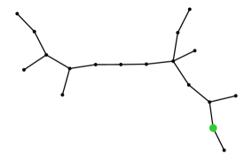
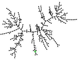
The transition from the quiescent to the chaotic phase can be understood from the underlying structure of connections. Due to the power-law connectivity density, we can expect that only a small fraction of the connections contribute to the activity profile of the network. Indeed, as we show in the following, the transition to chaos is driven by the percolation transition of autocrat connections for which , i.e. an active pre-synaptic neuron will activate the post-synaptic neuron in the absence of other inputs. Around the critical point the mean activity of the network is infinitesimal and thus the higher order interaction events (e.g. two neurons activating another neuron) are negligible. In other words, to a good approximation, a neuron can only be activated by another single neuron through an autocrat connection, independently from other neurons. This suggests that the transition to chaos in the neural network model is related to the critical branching processes Harris (2002) (Fig. 1).
In the Cauchy case the probability that a given connection is an autocrat reads
| (9) |
For a given neuron, the number of outgoing (or incoming) autocrat connections is a binomial random variable with trials and the probability of success given by (9). In the limit of it converges to the Poisson random variable with intensity
| (10) |
Now, let the initial state of the network be such that only a single neuron (seed) is active. The number of active neurons (descendants) in the next step is given by the Poisson distribution and the mean number of active neurons is given by (10). The theory of branching processes predicts that the population will eventually die out almost surely for and has a finite survival probability for . At the process is critical and features scale-free avalanches. The critical point predicted by the branching process formulation of the network dynamics, , is the same as the mean-field critical point predicted by (8).
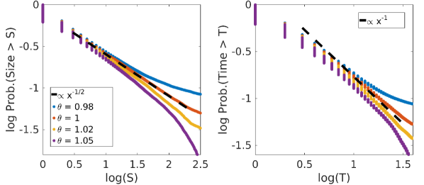
The mapping to the branching process explains many features of the Cauchy neural network around the critical point. Below the critical point the steady state is quiescent and a bit-flip perturbation corresponds to a single neuron (seed) being activated. The local expansion rate of such perturbation is given by . Above the critical point () each bit-flip contributes in the same manner as a single seed and, additionally, interacts with other active neurons to activate and deactivate other descendants. Thus, in the vicinity of the transition point gives a lower bound on the local expansion rate of a perturbation in the steady state, and for the network is expected to be chaotic in the thermodynamic limit SI . Moreover, the transition to chaos belongs to the mean-field directed percolation universality class Alstrøm (1988); Munoz et al. (1999); Ódor (2004). The propagation of the corresponding avalanches is characterized by SI power-law distributed sizes : , and power-law distributed lifetimes : . These theoretical predictions were corroborated by our computer simulations of the Cauchy network, as shown in Fig. 2.
For a comparison, we have also studied Gaussian networks of threshold units with a fixed number of connections per neuron SI ; Derrida et al. (1987). While extremely sparsely connected Gaussian networks () behave qualitatively similar to the Cauchy network, the transition to chaos becomes discontinuous in the biologically relevant regime of . With a biologically realistic and finite , the network activity jumps between two metastable states near the transition point, and cannot be robustly posed at the edge of chaos. The discontinuous property is due to the emergence of a metastable active state by the saddle-node bifurcation as increases.
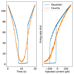
Importantly, although our theoretical predictions were derived assuming simplistic threshold neural units, they translate directly to networks of more biologically plausible leaky integrate-and-fire (LIF) neurons. The difference of continuous and discontinuous transition is confirmed by the presence or absence of a hysteresis loop in more realistic networks of LIF neurons (Fig. 3). Hence, unlike the Gaussian networks with realistic , Cauchy networks demonstrate critical phenomena and can reproduce experimentally observed scale-free avalanches at the critical point. Moreover, a large Cauchy network can exhibit arbitrarily low, self-sustained activity levels. In contrast, the lowest possible activity level that can be achieved by the Gaussian network with realistic is about in the binary case and in the LIF case (Fig. 3).
For clarity we chose to limit our presentation to the Cauchy distribution of , but our results naturally extend to other power-law distributions. Indeed, let the synaptic efficacy density asymptotically behave like a power-law 222 Note that we scale with the number of neurons as , which assures the existence of a non-trivial limit . For another choice is to scale the synaptic strengths as , which in the limit of corresponds to the Gaussian network. . We then have , which holds for large enough . The branching parameter is calculated as in (10) and reads . A continuous transition takes place at and its features are, as before, described by the directed percolation universality class.
The connectivity in the current model is unstructured. It would be interesting to combine power-law synaptic weight distributions with structured networks, for example, with hierarchical modules Friedman and Landsberg (2013) or oscillations Poil et al. (2012); di Santo et al. (2018); Fontenele et al. (2019).
Incidentally, the same Cauchy distribution of membrane potential was found in the quadratic integrate and fire neuron model Montbrió et al. (2015) due to single-neuron dynamics. Nontrivial effects may arise from a combination of single-neuron- and network-driven heavy-tail statistics.
Power-law distributions of synaptic weights feature many very weak synapses, that do not directly contribute to the computation. Even though this may seem wasteful, we think that such architectures are not only biologically plausible Cossell et al. (2015) but may be beneficial. One possibility is that even weak connections can activate a neuron once contextual input from another part of the brain increases the baseline membrane potential close to its spiking threshold. Such contextual input can also raise the spiking probability of nearby neurons so that synchronous activation of weak connections is more likely. Weak synapses have also been reported to play a role in unsupervised features extraction Huang (2018). In the context of reservoir computing Jaeger (2001); Maass et al. (2002) high computational capabilities were achieved using non-biologically sparse connectivity Büsing et al. (2010). Our model provides a more biologically plausible solution that the connectivity can be anatomically dense but effectively sparse due to heavy-tailed synaptic weight distribution. More generally, the optimal degree of sparsity depends on the role of a given brain structure and the type of the employed plasticity Litwin-Kumar et al. (2017). Power-law distributed synaptic weights may in this context provide a weakly informative Gelman et al. (2008); Van Dongen (2006) sparse-connectivity prior, with weak and effectively silent synapses providing a pool of potential connections that can be recruited when and if needed, as observed in the brain during development Liao et al. (1995); Kerchner and Nicoll (2008).
Our results demonstrate that the shape of the synaptic weight distribution can dramatically affect dynamics of neural networks. A biological distribution of synaptic weights can give distinct predictions from the frequently assumed Gaussian distribution. The proposed mathematical framework with power-law synaptic weights can easily be adapted to other scenarios in future studies.
Acknowledgements.
We thank Francesco Fumarola and anonymous referees for invaluable discussions and comments on the manuscript. Supported by RIKEN Center for Brain Science, Brain/MINDS from AMED under Grant Number JP20dm020700, and JSPS KAKENHI Grant Number JP18H05432.References
- Beggs and Plenz (2003) J. M. Beggs and D. Plenz, Journal of neuroscience 23, 11167 (2003).
- Shew et al. (2015) W. L. Shew, W. P. Clawson, J. Pobst, Y. Karimipanah, N. C. Wright, and R. Wessel, Nature Physics 11, 659 (2015).
- Fontenele et al. (2019) A. J. Fontenele, N. A. de Vasconcelos, T. Feliciano, L. A. Aguiar, C. Soares-Cunha, B. Coimbra, L. Dalla Porta, S. Ribeiro, A. J. Rodrigues, N. Sousa, et al., Physical review letters 122, 208101 (2019).
- Petermann et al. (2009) T. Petermann, T. C. Thiagarajan, M. A. Lebedev, M. A. Nicolelis, D. R. Chialvo, and D. Plenz, Proceedings of the National Academy of Sciences 106, 15921 (2009).
- Haldeman and Beggs (2005) C. Haldeman and J. M. Beggs, Physical review letters 94, 058101 (2005).
- Kinouchi and Copelli (2006) O. Kinouchi and M. Copelli, Nature physics 2, 348 (2006).
- di Santo et al. (2018) S. di Santo, P. Villegas, R. Burioni, and M. A. Muñoz, Proceedings of the National Academy of Sciences 115, E1356 (2018).
- Stoop and Gomez (2016) R. Stoop and F. Gomez, Physical review letters 117, 038102 (2016).
- Munoz (2018) M. A. Munoz, Reviews of Modern Physics 90, 031001 (2018).
- Langton (1990) C. G. Langton, Physica D: Nonlinear Phenomena 42, 12 (1990).
- Bertschinger and Natschläger (2004) N. Bertschinger and T. Natschläger, Neural computation 16, 1413 (2004).
- Legenstein and Maass (2007) R. Legenstein and W. Maass, New directions in statistical signal processing: From systems to brain , 127 (2007).
- Toyoizumi and Abbott (2011) T. Toyoizumi and L. Abbott, Physical Review E 84, 051908 (2011).
- Schuecker et al. (2018) J. Schuecker, S. Goedeke, and M. Helias, Physical Review X 8, 041029 (2018).
- Benayoun et al. (2010) M. Benayoun, J. D. Cowan, W. van Drongelen, and E. Wallace, PLoS computational biology 6, e1000846 (2010).
- Beggs and Timme (2012) J. M. Beggs and N. Timme, Frontiers in physiology 3, 163 (2012).
- Sompolinsky et al. (1988) H. Sompolinsky, A. Crisanti, and H.-J. Sommers, Physical review letters 61, 259 (1988).
- Molgedey et al. (1992) L. Molgedey, J. Schuchhardt, and H. G. Schuster, Physical review letters 69, 3717 (1992).
- Amit and Brunel (1997) D. J. Amit and N. Brunel, Cerebral cortex (New York, NY: 1991) 7, 237 (1997).
- Brunel (2000) N. Brunel, Journal of computational neuroscience 8, 183 (2000).
- Rajan et al. (2010) K. Rajan, L. Abbott, and H. Sompolinsky, Physical Review E 82, 011903 (2010).
- Massar and Massar (2013) M. Massar and S. Massar, Physical Review E 87, 042809 (2013).
- Stern et al. (2014) M. Stern, H. Sompolinsky, and L. Abbott, Physical Review E 90, 062710 (2014).
- Aljadeff et al. (2015) J. Aljadeff, M. Stern, and T. Sharpee, Physical review letters 114, 088101 (2015).
- Kadmon and Sompolinsky (2015) J. Kadmon and H. Sompolinsky, Physical Review X 5, 041030 (2015).
- Wainrib and Galtier (2016) G. Wainrib and M. N. Galtier, Neural Networks 76, 39 (2016).
- Crisanti and Sompolinsky (2018) A. Crisanti and H. Sompolinsky, Physical Review E 98, 062120 (2018).
- Harish and Hansel (2015) O. Harish and D. Hansel, PLoS computational biology 11 (2015).
- Dayan and Abbott (2001) P. Dayan and L. F. Abbott, (2001).
- Häusser and Monsivais (2003) M. Häusser and P. Monsivais, Neuron 40, 449 (2003).
- Gerstner et al. (2014) W. Gerstner, W. M. Kistler, R. Naud, and L. Paninski, Neuronal dynamics: From single neurons to networks and models of cognition (Cambridge University Press, 2014).
- Millman et al. (2010) D. Millman, S. Mihalas, A. Kirkwood, and E. Niebur, Nature physics 6, 801 (2010).
- Dayan and Abbott (2005) P. Dayan and L. F. Abbott, Theoretical Neuroscience: Computational and Mathematical Modeling of Neural Systems (The MIT Press, 2005).
- Marshel et al. (2019) J. H. Marshel, Y. S. Kim, T. A. Machado, S. Quirin, B. Benson, J. Kadmon, C. Raja, A. Chibukhchyan, C. Ramakrishnan, M. Inoue, et al., Science 365, eaaw5202 (2019).
- Scarpetta et al. (2018) S. Scarpetta, I. Apicella, L. Minati, and A. de Candia, Physical Review E 97, 062305 (2018).
- Sayer et al. (1990) R. Sayer, M. Friedlander, and S. Redman, Journal of Neuroscience 10, 826 (1990).
- Feldmeyer et al. (1999) D. Feldmeyer, V. Egger, J. Lübke, and B. Sakmann, The Journal of physiology 521, 169 (1999).
- Song et al. (2005) S. Song, P. J. Sjöström, M. Reigl, S. Nelson, and D. B. Chklovskii, PLoS biology 3, e68 (2005).
- Lefort et al. (2009) S. Lefort, C. Tomm, J.-C. F. Sarria, and C. C. Petersen, Neuron 61, 301 (2009).
- Ikegaya et al. (2012) Y. Ikegaya, T. Sasaki, D. Ishikawa, N. Honma, K. Tao, N. Takahashi, G. Minamisawa, S. Ujita, and N. Matsuki, Cerebral Cortex 23, 293 (2012).
- Loewenstein et al. (2011) Y. Loewenstein, A. Kuras, and S. Rumpel, Journal of Neuroscience 31, 9481 (2011).
- Gilson and Fukai (2011) M. Gilson and T. Fukai, PloS one 6, e25339 (2011).
- Zheng et al. (2013) P. Zheng, C. Dimitrakakis, and J. Triesch, PLoS computational biology 9, e1002848 (2013).
- Yasumatsu et al. (2008) N. Yasumatsu, M. Matsuzaki, T. Miyazaki, J. Noguchi, and H. Kasai, Journal of Neuroscience 28, 13592 (2008).
- Nagaoka et al. (2016) A. Nagaoka, H. Takehara, A. Hayashi-Takagi, J. Noguchi, K. Ishii, F. Shirai, S. Yagishita, T. Akagi, T. Ichiki, and H. Kasai, Scientific reports 6, 26651 (2016).
- Humble et al. (2019) J. Humble, K. Hiratsuka, H. Kasai, and T. Toyoizumi, Frontiers in Computational Neuroscience 13, 38 (2019).
- Ishii et al. (2018) K. Ishii, A. Nagaoka, Y. Kishida, H. Okazaki, S. Yagishita, H. Ucar, N. Takahashi, N. Saito, and H. Kasai, eNeuro 5 (2018).
- Okazaki et al. (2018) H. Okazaki, A. Hayashi-Takagi, A. Nagaoka, M. Negishi, H. Ucar, S. Yagishita, K. Ishii, T. Toyoizumi, K. Fox, and H. Kasai, Neuroscience letters 671, 99 (2018).
- Teramae et al. (2012) J.-n. Teramae, Y. Tsubo, and T. Fukai, Scientific reports 2, 485 (2012).
- Buzsáki and Mizuseki (2014) G. Buzsáki and K. Mizuseki, Nature Reviews Neuroscience 15, 264 (2014).
- Teramae and Fukai (2014) J.-n. Teramae and T. Fukai, Proceedings of the IEEE 102, 500 (2014).
- Omura et al. (2015) Y. Omura, M. M. Carvalho, K. Inokuchi, and T. Fukai, Journal of Neuroscience 35, 14585 (2015).
- Feller (1971) W. Feller, An introduction to probability and its applications, Vol. II (Wiley, New York, 1971).
- Cizeau and Bouchaud (1994) P. Cizeau and J.-P. Bouchaud, Physical Review E 50, 1810 (1994).
- Burda et al. (2002) Z. Burda, R. A. Janik, J. Jurkiewicz, M. A. Nowak, G. Papp, and I. Zahed, Physical Review E 65, 021106 (2002).
- Gudowska-Nowak et al. (2020) E. Gudowska-Nowak, M. A. Nowak, D. R. Chialvo, J. K. Ochab, and W. Tarnowski, Neural Computation 32, 395 (2020).
- (57) See Supplementary Material for details, which includes Refs. Goles (1986); Bezanson et al. (2017); Linssen et al. (2018).
- Note (1) In the binary case the system has a finite number of states for any finite and the attractor has to be periodic. Thus, formally, irregular aperiodic behavior can only be observed in the limit of . Chaos-like signatures can nonetheless be observed for finite , e.g. the typical lengths of transients and cycles rapidly change around the predicted transition point, and grow exponentially with in the “chaotic” phase Vreeswijk and Sompolinsky (1998); Luque and Solé (2000).
- Harris (2002) T. E. Harris, The theory of branching processes (Courier Corporation, 2002).
- Alstrøm (1988) P. Alstrøm, Physical Review A 38, 4905 (1988).
- Munoz et al. (1999) M. A. Munoz, R. Dickman, A. Vespignani, and S. Zapperi, Physical Review E 59, 6175 (1999).
- Ódor (2004) G. Ódor, Reviews of modern physics 76, 663 (2004).
- Derrida et al. (1987) B. Derrida, E. Gardner, and A. Zippelius, EPL (Europhysics Letters) 4, 167 (1987).
- Note (2) Note that we scale with the number of neurons as , which assures the existence of a non-trivial limit . For another choice is to scale the synaptic strengths as , which in the limit of corresponds to the Gaussian network.
- Friedman and Landsberg (2013) E. J. Friedman and A. S. Landsberg, Chaos: An Interdisciplinary Journal of Nonlinear Science 23, 013135 (2013).
- Poil et al. (2012) S.-S. Poil, R. Hardstone, H. D. Mansvelder, and K. Linkenkaer-Hansen, Journal of Neuroscience 32, 9817 (2012).
- Montbrió et al. (2015) E. Montbrió, D. Pazó, and A. Roxin, Physical Review X 5, 021028 (2015).
- Cossell et al. (2015) L. Cossell, M. F. Iacaruso, D. R. Muir, R. Houlton, E. N. Sader, H. Ko, S. B. Hofer, and T. D. Mrsic-Flogel, Nature 518, 399 (2015).
- Huang (2018) H. Huang, Journal of Physics A: Mathematical and Theoretical 51, 08LT01 (2018).
- Jaeger (2001) H. Jaeger, Bonn, Germany: German National Research Center for Information Technology GMD Technical Report 148, 13 (2001).
- Maass et al. (2002) W. Maass, T. Natschläger, and H. Markram, Neural computation 14, 2531 (2002).
- Büsing et al. (2010) L. Büsing, B. Schrauwen, and R. Legenstein, Neural computation 22, 1272 (2010).
- Litwin-Kumar et al. (2017) A. Litwin-Kumar, K. D. Harris, R. Axel, H. Sompolinsky, and L. Abbott, Neuron 93, 1153 (2017).
- Gelman et al. (2008) A. Gelman, A. Jakulin, M. G. Pittau, Y.-S. Su, et al., The Annals of Applied Statistics 2, 1360 (2008).
- Van Dongen (2006) S. Van Dongen, Journal of Theoretical Biology 242, 90 (2006).
- Liao et al. (1995) D. Liao, N. A. Hessler, and R. Malinow, Nature 375, 400 (1995).
- Kerchner and Nicoll (2008) G. A. Kerchner and R. A. Nicoll, Nature Reviews Neuroscience 9, 813 (2008).
- Goles (1986) E. Goles, Discrete Applied Mathematics 13, 97 (1986).
- Bezanson et al. (2017) J. Bezanson, A. Edelman, S. Karpinski, and V. B. Shah, SIAM review 59, 65 (2017).
- Linssen et al. (2018) C. Linssen, M. E. Lepperød, J. Mitchell, J. Pronold, J. M. Eppler, C. Keup, A. Peyser, S. Kunkel, P. Weidel, Y. Nodem, D. Terhorst, R. Deepu, M. Deger, J. Hahne, A. Sinha, A. Antonietti, M. Schmidt, L. Paz, J. Garrido, T. Ippen, L. Riquelme, A. Serenko, T. Kühn, I. Kitayama, H. Mørk, S. Spreizer, J. Jordan, J. Krishnan, M. Senden, E. Hagen, A. Shusharin, S. B. Vennemo, D. Rodarie, A. Morrison, S. Graber, J. Schuecker, S. Diaz, B. Zajzon, and H. E. Plesser, “Nest 2.16.0,” (2018).
- Vreeswijk and Sompolinsky (1998) C. v. Vreeswijk and H. Sompolinsky, Neural computation 10, 1321 (1998).
- Luque and Solé (2000) B. Luque and R. V. Solé, Physica A: Statistical Mechanics and its Applications 284, 33 (2000).
See pages ,1,,2,,3,,4,,5,,6,,7 of SM.pdf