Constraining the magnetic field structure in collisionless relativistic shocks with a radio afterglow polarization upper limit in GW 170817

Abstract

Gamma-ray burst (GRB) afterglow arises from a relativistic shock driven into the ambient medium, which generates tangled magnetic fields and accelerates relativistic electrons that radiate the observed synchrotron emission. In relativistic collisionless shocks the postshock magnetic field B is produced by the two-stream and/or Weibel instabilities on plasma skin-depth scales $(c/\omega_{p})$, and is oriented predominantly within the shock plane ($B_{\perp}$; transverse to the shock normal, $\hat{\textbf{{n}}}_{\rm{sh}}$), and is often approximated to be completely within it ($B_{\parallel}\equiv\hat{\textbf{{n}}}_{\rm{sh}}\,\cdot\,\textbf{{B}}=0$). Current 2D/3D particle-in-cell simulations are limited to short timescales and box sizes $\lesssim 10^{4}(c/\omega_{p})\ll R/\Gamma_{\rm{sh}}$ much smaller than the shocked region’s comoving width, and hence cannot probe the asymptotic downstream B structure. We constrain the latter using the linear polarization upper limit, $|\Pi|<12\%$, on the radio afterglow of GW 170817 / GRB 170817A. Afterglow polarization depends on the jet’s angular structure, our viewing angle, and the B structure. In GW 170817 / GRB 170817A the latter can be tightly constrained since the former two are well-constrained by its exquisite observations. We model B as an isotropic field in 3D that is stretched along $\hat{\textbf{{n}}}_{\rm{sh}}$ by a factor $\xi\equiv{}B_{\parallel}/B_{\perp}$, whose initial value $\xi_{f}\equiv{}B_{\parallel,f}/B_{\perp,f}$ describes the field that survives downstream on plasma scales $\ll{}R/\Gamma_{\rm{sh}}$. We calculate $\Pi(\xi_{f})$ by integrating over the entire shocked volume for a Gaussian or power-law core-dominated structured jet, with a local Blandford-McKee self-similar radial profile (used for evolving $\xi$ downstream). We find that independent of the exact jet structure, B has a finite, but initially sub-dominant, parallel component: $0.57\lesssim\xi_{f}\lesssim 0.89$, making it less anisotropic. While this motivates numerical studies of the asymptotic B structure in relativistic collisionless shocks, it may be consistent with turbulence amplified magnetic field.

1 Introduction

There is good evidence that synchrotron radiation is the dominant emission mechanism in most GRB afterglows (e.g., Mészáros & Rees 1997; Waxman 1997; Sari et al. 1998, and see Piran 2004; Kumar & Zhang 2015 for a review). However, it depends on the rather poorly understood physics of relativistic collisionless shocks, in particular the microphysical processes that accelerate particles into a non-thermal energy distribution and generate near-equipartition tangled magnetic fields just behind the shock. These uncertainties are generally parameterized using the microphysical parameters, $\epsilon_{e}=\langle\gamma_{e}\rangle\rho_{e}c^{2}/e$ and $\epsilon_{B}=B^{2}/8\pi e$, that define the fraction of the total comoving internal energy density behind the afterglow shock, $e$, given to non-thermal relativistic electrons, with mean energy per unit rest-mass energy $\langle\gamma_{e}\rangle\gg 1$ and comoving rest-mass density $\rho_{e}$, and to the magnetic field of strength $B$, respectively (where all of these quantities are measured in the downstream comoving rest frame, and $c$ is the speed of light). Detailed works comparing this synchrotron shock model with GRB afterglow observations find $\epsilon_{e}\sim 10^{-1}$ and a wide range for $\epsilon_{B}\sim 10^{-5}-10^{-1}$ (e.g., Wijers & Galama 1999; Panaitescu & Kumar 2002; however also see Santana et al. 2014 who find $\epsilon_{B}$ values smaller by at least a factor of $10^{-2}$). These represent the emissivity-weighted mean values of the microphysical parameters assuming a uniform emission region, and do not account for their possible variation within the shocked region.

The leading theoretical explanation for magnetic field generation at the collisionless relativistic forward shock posits that when the upstream plasma into which the shock is expanding is weakly magnetized or unmagnetized (with a magnetization parameter $\sigma=B^{2}/4\pi\rho c^{2}\lesssim 10^{-3}$), magnetic fields are produced by the relativistic two-stream and/or Weibel (filamentation) instabilities (Weibel, 1959; Gruzinov & Waxman, 1999; Medvedev & Loeb, 1999; Bret, 2009; Keshet et al., 2009; Nakar et al., 2011). The shock-accelerated supra-thermal particles that escape into the upstream plasma and propagate ahead of the shock excite micro-instabilities in a spatially extended region called the precursor. These micro-instabilities (e.g. the Weibel-filamentation) generate a magnetic barrier at the proton skin-depth scales of $c/\omega_{p}=2.3\times 10^{7}n_{0}^{-1/2}\,$cm, where $c$ is the speed of light, $\omega_{p}$ is the proton plasma frequency, and $n_{0}=n/(1~{}{\rm cm}^{-3})$ is the upstream particle number density, which grows to near-equipartition with $\epsilon_{B}\sim 10^{-2}-10^{-1}$ and isotropizes the incoming plasma (Moiseev & Sagdeev 1963; see, e.g. Sironi et al. 2015 for a review). The generated field is randomly oriented but lies predominantly in the plane transverse to the direction of shock propagation. Since the size of the emission region (below the cooling frequency) in the comoving frame $\Delta_{\rm sh}^{\prime}$ is much larger, with $(c/\omega_{p})\ll\Delta_{\rm sh}^{\prime}\sim R/\Gamma_{\rm sh}=10^{14}R_{15}\Gamma_{\rm sh,1}^{-1}\,$cm where $R$ and $\Gamma_{\rm sh}$ are, respectively, the radial distance and Lorentz factor (LF) of the shock, the field must be able to survive much deeper downstream of the shock (Piran, 2005) without completely decaying due to particle phase-space mixing (Gruzinov, 2001).

Numerical simulations and analytic works show that the coherence scale of the magnetic field grows beyond the skin-depth scales via the formation of current filaments (Silva et al., 2003; Frederiksen et al., 2004; Medvedev et al., 2005). However, these may be subject to pressure-driven instabilities, e.g. the kink instability, which would destroy the filamentary structure, thermalize the particles, and cause the field to decay in the shocked region (Milosavljević & Nakar, 2006). 2D $e^{\pm}$-pair plasma PIC simulations (Chang et al., 2008; Spitkovsky, 2008a) and 2.5D electron-ion PIC simulations (Spitkovsky, 2008b) have also found that the filaments break up into clumps surrounded by a highly isotropic plasma and the magnetic field rapidly decays after $\sim$few$\,\times\,100\,(c/\omega_{p,e})$, with $\omega_{p,e}$ being the electron plasma frequency, and $\sim 20(c/\omega_{p})$, respectively. Many of these results are derived from the short-term evolution of the shock structure and the downstream magnetic field. Long-term PIC simulations (e.g., Keshet et al., 2009) instead find that at times $t>10^{3}\omega_{p,e}^{-1}$ the properties of the shock and current filaments in the precursor region are gradually modified by shock-accelerated energetic particles. This causes a gradual increase in the level of magnetization and the magnetic field coherence scale in the upstream. Consequently, as the magnetic field advects into the downstream, the decay rate of the postshock magnetic field slows down, its coherence length grows, and $\epsilon_{B}$ approaches $\sim 10^{-2}$ on length scales up to $\sim 10^{3}c/\omega_{p,e}$ downstream of the shock transition.

Synchrotron radiation is partially linearly polarized, and therefore, measurement of linear polarization of GRB afterglows is an invaluable tool to study the asymptotic structure of the postshock magnetic field. However, the emergent polarization depends not only on the magnetic field structure but also on the structure of the jet and the observer’s line-of-sight (LOS), leading to considerable degeneracy for an off-axis ($\theta_{\rm obs}>0$) observer. To break the degeneracy between the magnetic field structure, the jet structure and $\theta_{\rm obs}$, it is important to first independently model the latter two using the afterglow lightcurve and image on the plane of the sky. In this work, we use the exquisite broadband afterglow observations of GW 170817 / GRB 170817A and the semi-analytic model fits (from afterglow data up to $t_{\rm obs}\sim 600\,$ days) obtained by Gill & Granot (2018); Gill et al. (2019) for axi-symmetric core-dominated jet angular structures. These models for the jet’s angular structure and $\theta_{\rm obs}$ are then used to predict the degree of linear polarization for different tangled postshock magnetic fields, which are naturally symmetric with respect to $\hat{\textbf{{n}}}_{\rm sh}$. Finally, our model predictions are compared to the polarization upper limit for GW 170817 / GRB 170817A to constrain the postshock magnetic field structure.

The rest of the paper is organized as follows. In §2, we first present a general discussion of how linear polarization is produced in axisymmetric flows from different magnetic field configurations and jet structures. Then, we briefly discuss how afterglow observations of GW 170817 / GRB 170817A were used to constrain the jet structure and $\theta_{\rm obs}$. In §3 we describe the jet structure and dynamics used in this work, which features an angular structure given by two semi-analytic models of core-dominated structured jets with local spherical dynamics (see Gill & Granot, 2018, for more details) superimposed with a Blandford & McKee (1976) radial profile for the postshock flow. In §4, in order to calculate the linear polarization, we model the postshock magnetic field B and parameterize its degree of anisotropy through $\xi\equiv{}B_{\parallel}/B_{\perp}$, whose initial value $\xi_{f}\equiv{}B_{\parallel,f}/B_{\perp,f}$ describes the field that survives downstream on plasma scales $\ll{}R/\Gamma_{\rm{sh}}$. Since each fluid element is stretched more along the shock normal direction $\hat{\textbf{{n}}}_{\rm sh}$ than in the two perpendicular directions as it flows downstream, $\xi$ grows with the distance behind the shock. In §5 we obtain strong constraints on the shock-generated field anisotropy just behind the shock (namely $0.57\lesssim\xi_{f}\lesssim 0.89$) by comparing the predicted degree of polarization to the radio upper limit. Finally, in §6 we discuss the important implications that this result may have for the magnetic fields generated in relativistic collisionless shocks. Our results strongly suggest that the shock-generated field must have a component parallel to the shock normal and it cannot be only in the plane transverse to it, as suggested in earlier works (e.g., Medvedev & Loeb, 1999). We find the postshock field to be less anisotropic, which may be consistent with a turbulence amplified magnetic field.

Throughout this work, the notation $Q_{x}$ denotes the value of the quantity $Q$ in units of $10^{x}$ times its (cgs) units.

2 Linear polarization of GRB afterglows: magnetic field and jet structures

Here we summarize the different ways in which net linear polarization is obtained in GRB afterglows. We point out the degeneracy between different magnetic field configurations that can potentially lead to similar levels of polarization. This is further complicated by the degeneracy between the magnetic field configuration, jet structure and viewing angle $\theta_{\rm obs}$, where off-axis viewing ($\theta_{\rm obs}>0$) breaks the symmetry of the image for an axisymmetric flow, leading to net polarization.

Since GRBs are cosmological sources and their images on the plane of the sky are generally unresolved, any measurement of linear polarization effectively averages the local polarization over the entire image. As a result, linear polarization from shock-generated fields, which are on average symmetric around the local shock normal direction, $\hat{\textbf{{n}}}_{\rm{sh}}$ (as it is the only relevant preferred direction locally), would average out for a spherical flow and produce no net polarization (as there would be no global preferred direction). Therefore, in order to detect any residual polarization, the symmetry of the image must be broken. For a spherical flow this can occur if different weight is given to different parts of the image, e.g. through microlensing (Loeb & Perna, 1998), radio scintillations (Medvedev & Loeb, 1999), clumps in the external medium (Granot & Königl, 2003), or angular inhomogeneities in the jet (“patchy shell”, Kumar & Piran, 2000; Ioka & Nakamura, 2001; Granot & Königl, 2003; Nakar & Oren, 2004; Yamazaki et al., 2004). However, these are expected to occur only in some fraction of GRB afterglow, and would be accompanied by temporal variability in the afterglow lightcurve that was not observed in GRB 170817A.

A more robust and therefore also more popular way of breaking the symmetry of the afterglow image is through an axisymmetric flow (i.e. a jet) observed off-axis (from $\theta_{\rm obs}>0$, where $\theta_{\rm obs}$ is measured from the jet’s symmetry axis). This can occur in two ways: (i) if the emission arises from a relativistic (with LF $\Gamma\gg 1$) uniform jet with sharp edges at an initial half-opening angle $\theta_{0}$ (i.e. a “top-hat” jet), an off-axis observer within the jet’s aperture ($0<\theta_{\rm{obs}}<\theta_{0}$) sees the edge of the jet near the time of the jet break in the lightcurve, when the flow decelerates so that the beaming cone of the emission widens to $1/\Gamma\gtrsim(\theta_{0}-\theta_{\rm obs})$ (Ghisellini & Lazzati, 1999; Sari, 1999). This results in incomplete cancellation of polarization which yields finite residual polarization when averaged over the GRB image; (ii) If the flow is structured and its properties, e.g. the energy per unit solid angle and/or Lorentz factor, vary with polar angle $\theta$ from the jet symmetry axis (i.e. a “structured” jet, e.g. Kumar & Granot, 2003), the gradient in the polarized intensity in the observed region again leads to incomplete cancellation of polarization (Rossi et al., 2004; Gill & Granot, 2018).

Alternatively, net polarization is obtained if the shocked region is permeated by an ordered magnetic field component in addition to the shock-generated random field (Granot & Königl, 2003), or if the emission region consists of coherent magnetic field patches (Gruzinov & Waxman, 1999) of angular scale $\theta_{B}<1/\Gamma$, such that the image (i.e. the observed region of angle $\sim 1/\Gamma$ around our line of sight) contains $N\sim(\Gamma\theta_{B})^{2}$ patches. In these two cases, the symmetry is broken by the ordered field component, for which the local maximum polarization is $0.5\leq[\Pi_{\max}=(\alpha+1)/(\alpha+5/3)]\lesssim 0.75$ where $\alpha=-d\log F_{\nu}/d\log\nu$ is the spectral index. In the $N$-patches model, since the emission arises from $N$ intrinsically coherent but mutually incoherent patches, the net polarization is reduced to $\Pi\sim\Pi_{\max}/\sqrt{N}$ due to partial cancellation (the $\sqrt{N}$ suppression factor arising from random walk in the Stokes parameters ($U,\,Q$) plane).

Measurement of $\Pi\sim 1\%-3\%$ in the optical and NIR afterglow of several GRBs (e.g., Covino et al. 1999; Wijers et al. 1999, also see Covino & Gotz 2016 for a review) confirmed the synchrotron origin of the emission. Such low levels of polarization readily ruled out an ordered magnetic field with coherence angular scale $\theta_{B}\gtrsim 1/\Gamma$. Instead, they suggested either ordered fields with much smaller coherence length scales, as in the $N$-patches scenario, or shock-generated tangled fields. In the latter case, however, the magnetic field must have some level of anisotropy if the flow is uniform or the GRB image must be inhomogeneous owing to the fact that the observer is off-axis and the jet either has a sharp edge or a core-dominated angular structure. Granot & Königl (2003) parameterized the postshock tangled magnetic field anisotropy using $b\equiv 2\langle B_{\parallel}^{2}\rangle/\langle B_{\perp}^{2}\rangle$, the ratio of the radially averaged energy densities of the two field components. Note that $b=1$ for a field that is isotropic in 3D and gives zero local polarization, so the closer $b$ is to one the lower the local and global degrees of polarizations. Using the observed levels of afterglow polarization $\Pi\sim 1\%-3\%$ around several hours to a few days, which were relatively close to the jet break time around which the polarization is expected to peak, and assuming emission from an infinitely thin relativistic spherical shell, Granot & Königl (2003) constrained $b$ to be approximately within the range $0.5\lesssim b\lesssim 2$. This involved a statistical argument about the distribution of $\theta_{\rm obs}$ between the different GRBs within the modest sized sample with afterglow polarization measuremants that was available in 2003. Nevertheless, it already suggested that the postshock magnetic field must be at least mildly anisotropic.

Still, considerable degeneracy remains between the scenarios mentioned above and one way to break that is by the observation of the temporal evolution of the polarization position angle (PA), $\theta_{p}$. In the $N$-patches case, $\theta_{p}$ is expected to vary randomly and $\Pi$ fluctuates and gradually decreases, both over timescales $\Delta t\sim t$, as the visible region grows and encompasses more patches. Interestingly, both of these tell-tale signatures were recently observed by ALMA at $97\;$GHz in the reverse-shock emission (from the shocked original GRB ejecta) of GRB 190114C between 2.2 and 5.2 hours after the GRB, implying $\theta_{B}\sim 10^{-3}\;$rad (Laskar et al., 2019). On the other hand, for a mildly anisotropic shock generated magnetic field, $\theta_{p}$ flips by $90^{\circ}$ as $\Pi$ momentarily vanishes, around the time of the jet-break for a top-hat jet viewed off-axis (Ghisellini & Lazzati, 1999; Sari, 1999; Granot & Königl, 2003); for a structured jet viewed off-axis $\theta_{p}$ remains unchanged (Rossi et al., 2004).

Since $\theta_{\rm obs}$, the jet angular structure and the degree of anisotropy of the shock-generated magnetic field, all affect the observed polarization, it becomes important to model the angular structure of the flow, and constrain $\theta_{\rm{obs}}$. Almost all GRBs, whether of the long-soft or short-hard classes, have been observed at cosmological distances, which guarantees that the observer’s LOS lies within the beaming cone of the compact core of half-opening angle $\theta_{c}$, such that $\theta_{\rm obs}-\theta_{c}\lesssim\rm{few}\times\Gamma^{-1}$ for core-dominated jets where the emission sharply drops at $\theta>\theta_{c}$. This makes it challenging to draw any useful inferences on the jet structure and on our viewing angle $\theta_{\rm obs}$.

The afterglow of the short-hard GRB 170817A (Abbott et al., 2017b), associated to the first-ever detection of a binary neutron star merger gravitational wave source GW 170817 (Abbott et al., 2017a), has provided a golden opportunity to study the structure of outflows that power short-hard GRBs. The broadband afterglow, detected after $8.9\,$days in X-rays (Troja et al., 2017) and $16.4\,$days in the radio (Hallinan et al., 2017), showed an unusually long-lasting flux rise, as $F_{\nu}(t_{\rm{obs}})\propto\nu^{-0.6}t_{\rm{obs}}^{0.8}$, up to the peak at $t_{\rm{obs,pk}}\sim 150\,$days post merger (e.g. Lyman et al., 2018; Margutti et al., 2018; Mooley et al., 2018a), followed by a sharp decay as $F_{\nu}\propto{}t_{\rm{obs}}^{a}$ where $a\simeq-2$ (Mooley et al., 2018b; van Eerten et al., 2018; Hajela et al., 2019; Lamb et al., 2019). Several numerical and semi-analytic works modeled the afterglow as arising from a successful (i.e. bore its way through the merger dynamical ejecta rather than being chocked within it) off-axis core-dominated structured jet, whose angular profile is consistent with either a (quasi-) Gaussian or a narrow core with sharp power-law wings (Alexander et al., 2018; Lamb & Kobayashi, 2018; Lazzati et al., 2018; Nynka et al., 2018; Troja et al., 2017; D’Avanzo et al., 2018; Gill & Granot, 2018; Lyman et al., 2018; Margutti et al., 2018; Resmi et al., 2018; Troja et al., 2018; Hajela et al., 2019; Lamb et al., 2019). Later radio VLBI observations measured an apparent superluminal motion of the afterglow flux centroid with $\varv_{\rm app}\approx 4c$ (Mooley et al., 2018b), and constrained the angular size of the afterglow image on the plane of the sky to $\lesssim 2\,$mas (Ghirlanda et al., 2019; Mooley et al., 2018b). The apparent superluminal motion firmly established the fact that the outflow had a narrow relativistic compact core surrounded by low energy wings, which is consistent with the upper limit on its angular size.

Using VLA radio observations at $2.8\;$GHz an upper limit of $|\Pi|<12\%$ ($99\%$ confidence) was obtained on the afterglow linear polarization at $t_{\rm obs}\approx 244\,$days (Corsi et al., 2018). Comparison with detailed predictions for the linear polarization from semi-analytic models of core-dominated structured jets that explained the afterglow lightcurve and image size of GW 170817/GRB 170817A (Gill & Granot, 2018), revealed that $0.7\lesssim b\lesssim 1.5$, suggesting that the postshock magnetic field must be at most mildly anisotropic with a finite magnetic field component in the direction of the shock normal that is comparable to the components in the two perpendicular directions (Corsi et al., 2018; Gill et al., 2018). Having constrained the jet structure and viewing angle from the afterglow lightcurve and image properties of GW 170817 / GRB 170817A , this new tighter constraint on $b$ was free of any model degeneracy due to the jet structure and provided a robust estimate of the radially averaged magnetic field anisotropy. This severely constrained models of Weibel-instability-generated fields at collisionless shocks, where the field lies completely in the plane transverse to the shock normal. However, the calculation in Gill & Granot (2018) did not account for the radial structure of the flow and it effects on the magnetic field structure, since they adopted the thin-shell approximation. Therefore, the upper limit on linear polarization could only be used to constrain the radially averaged degree of anisotropy.

The GW 170817 / GRB 170817A  broadband afterglow spectrum was explained by a single power law segment (PLS) of synchrotron emission – PLS G (Granot & Sari, 2002) with spectral index $\alpha=(p-1)/2$ (with $F_{\nu}\propto\nu^{-\alpha}$ and power-law relativistic electron distribution $N(\gamma)\propto\gamma^{-p}$). In PLS G the emission is from slow-cooling electrons and hence it arises from the entire shocked volume behind the forward shock. Therefore, in this work we obtain the afterglow linear polarization by integrating over the entire emitting volume behind the forward shock.

3 Core-dominated angular structured flow with Blandford-McKee radial profile

We consider a core-dominated structured jet (e.g., Mészáros et al., 1998) with energy per unit solid angle, $\mathcal{E}(\theta)\equiv dE(\theta)/d\Omega$, and initial bulk $\Gamma_{0}(\theta)$ of the shocked material just behind the shock front, both declining with the polar angle $\theta$ from the jet symmetry axis (see Fig. 1). Here we consider two distinct angular profiles: (i) A Gaussian jet (GJ) for which both $\mathcal{E}(\theta)$ and the initial kinetic energy per unit rest mass, $\Gamma_{0}(\theta)-1$, have a Gaussian profile (Zhang & Mészáros, 2002; Kumar & Granot, 2003; Rossi et al., 2004) with a floor at $\theta=\theta_{*}$ corresponding to $\beta_{0}=\beta_{\rm min}=0.01$,

$$({\rm GJ})\quad\quad\frac{\mathcal{E}(\theta)}{\mathcal{E}_{c}}=\frac{\Gamma_{0}(\theta)-1}{\Gamma_{c}-1}=\exp\left[-\frac{1}{2}\left(\frac{\min\{\theta,\,\theta_{*}\}}{\theta_{c}}\right)^{2}\right]~{},$$ (1)

where $\mathcal{E}_{c}$ and $\Gamma_{c}$ represent the core values, and (ii) a Power-law jet (PLJ) for which both $\mathcal{E}(\theta)$ and $\Gamma_{0}(\theta)-1$ decline as a power law outside of the core,

$$({\rm PLJ})\quad\ \ \frac{\mathcal{E}(\theta)}{\mathcal{E}_{c}}=\Theta^{-a},\quad\ \ \frac{\Gamma_{0}(\theta)-1}{\Gamma_{c}-1}=\Theta^{-b},\quad\ \ \Theta=\sqrt{1+\left(\frac{\theta}{\theta_{c}}\right)^{2}}~{},$$ (2)

with their respective power law indices, $a$ and $b$.

For the dynamics, we neglect sideways expansion (or any temporal evolution of $\mathcal{E}(\theta)$), and assume that each point on the shock front expands locally only radially as part of a spherical flow with the local value of $\mathcal{E}(\theta)$. The rest mass density of the circumburst medium (CBM) is assumed to vary as a power-law with the radial distance $r$ from the central source, $\rho_{k}(r)=m_{p}n(r)=A_{k}r^{-k}$, where $k=0$ for a uniform density interstellar medium (ISM) and $k=2$ for a steady wind medium, $n(r)$ is the CBM particle number density, and $m_{p}$ is the proton mass. When the forward shock reaches a radius $r$, the corresponding spherical flow would have swept up a mass $m(r)=[4\pi A/(3-k)]r^{3-k}$, and since $m(r)$ increase with $r$ this decelerates the shock. A wind-like environment ($k=2$) is only relevant for GRBs of the long-soft class, where quasi-steady mass loss due to stellar winds from the progenitor star may be expected. In the case of BNS mergers, which is relevant for this work, a uniform ISM-like CBM ($k=0$) is expected.

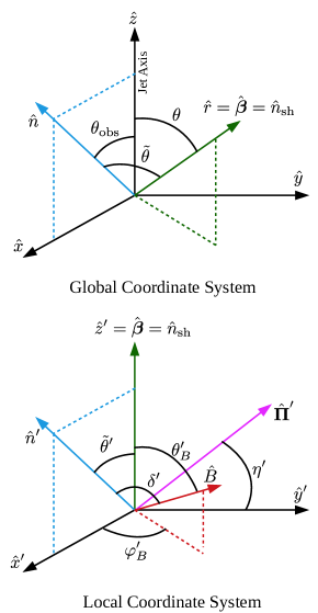
Figure 1: The global (lab-frame) and local (comoving-frame) coordinate systems, where the former is used to describe the structure of the jet, and the latter is used to describe the local magnetic field and is used in the calculation of linear polarization.

At an early stage, the shell is assumed to coast at a constant proper velocity $u_{0}(\theta)=\Gamma_{0}(\theta)\beta_{0}(\theta)$ until the deceleration radius, which is expressed as

$$R_{d}(\theta)=\left[\frac{(3-k)E_{\rm k,iso}(\theta)}{4\pi Ac^{2}u_{0}^{2}(\theta)}\right]^{1/(3-k)}~{}.$$ (3)

At the deceleration radius most of the isotropic equivalent energy of the blast wave, $E_{\rm k,iso}(\theta)=4\pi\mathcal{E}(\theta)$, is used up to accelerate the swept up mass to $u\approx u_{0}(\theta)$, and also to heat it up to a similar thermal proper velocity, so that $m[r_{d}(\theta)]u_{0}(\theta)c^{2}=E_{\rm k,iso}(\theta)$. Beyond this radius, the shell starts to decelerate as it continues to sweep up more mass and its dynamical evolution becomes self-similar, such that $u(\theta)\propto r^{-(3-k)/2}$, which is valid not only in the relativistic phase but also in the Newtonian Sedov-Taylor phase. During this deceleration phase, the dynamically averaged bulk LF of the postshock material can be expressed as (Panaitescu & Kumar, 2000; Gill & Granot, 2018)

$$\tilde{\Gamma}(\theta,\tilde{r})=\frac{\Gamma_{0}(\theta)+1}{2\,\tilde{r}^{\,3-k}}\left[\sqrt{1+\frac{4\Gamma_{0}(\theta)}{\Gamma_{0}(\theta)+1}\tilde{r}^{\,3-k}+\left(\frac{2\tilde{r}^{\,3-k}}{\Gamma_{0}(\theta)+1}\right)^{2}}-1\right]~{},$$ (4)

where $\tilde{r}=R/R_{d}(\theta)$. This estimate is particularly useful when the radiating electrons in the shocked material are fast cooling so that the lab-frame size of the emission region is much smaller than the width of the shocked region, $\Delta_{\gamma}\ll\Delta_{\rm sh}\sim R/\Gamma_{\rm sh}^{2}$. In this case, the emission region is generally approximated as being infinitely thin with bulk LF of the shell given by Eq. (4). From the Blandford & McKee (1976, BM76 hereafter) solution, the LF of the material just behind the shock is given by $\Gamma_{f}=[(17-4k)/4(3-k)]^{1/2}\tilde{\Gamma}$. Here and what follows, the subscript $f$ indicates the magnitude of any quantity just behind the shock front. So that the expression for $\Gamma_{f}$ remains valid in the non-relativistic regime as well, we use more generally $u_{f}=\Gamma_{f}\beta_{f}=(\Gamma_{f}^{2}-1)^{1/2}=[(17-4k)/4(3-k)]^{1/2}\tilde{u}$, where $\tilde{u}=\tilde{\Gamma}\,\tilde{\beta}$. The LF of the shock front is then given by (BM76)

$$\Gamma_{\rm sh}^{2}=\frac{(\Gamma_{f}+1)[\hat{\gamma}_{f}(\Gamma_{f}-1)+1]^{2}}{\hat{\gamma}_{f}(2-\hat{\gamma}_{f})(\Gamma_{f}-1)+2}\approx 2\Gamma_{f}^{2}\quad{\rm for}\quad\Gamma_{f}\gg 1\,,$$ (5)

where the adiabatic index $\hat{\gamma}_{f}=4/3~{}(5/3)$ for a relativistic (Newtonian) shock.

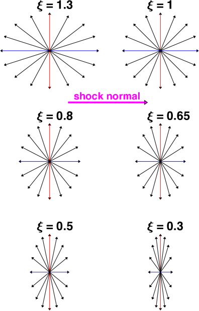
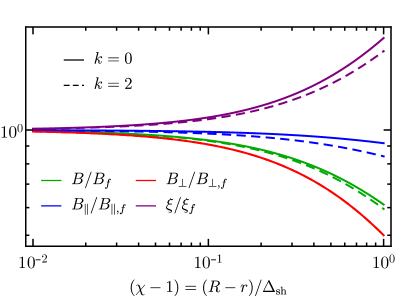
Figure 2: Top: Schematic of postshock magnetic field geometry for different values of the anisotropy parameter $\xi=B_{\parallel}/B_{\perp}=\xi_{f}\,\chi^{(7-2k)/(8-2k)}$. Bottom: Magnetic field radial profile shown as a function of the radial distance behind the shock, $(R-r)$, normalized by the lab-frame width of the shocked region, $\Delta_{\rm sh}\equiv R/[2(4-k)\Gamma_{\rm sh}^{2}]$. Here $r$ is the radial coordinate and $R$ is the radial distance of the shock front. All quantities are normalized by their value immediately behind the shock.

When the postshock electrons that dominate the emission in the observed frequency range are slow cooling (i.e. cool on a timescale larger than the dynamical time), then the emission is no longer limited to a very thin layer behind the forward shock. Instead, it arises from a larger volume of the shocked region, containing most of the energy and swept-up mass. In this case, it becomes important to know the properties of the emitting material downstream of the shock. It was shown by BM76 that at $R>R_{d}$ the dynamics of a spherical blast wave become self-similar, such that the radial profile of the postshock fluid can be described using a similarity variable

$$\chi=1+2(4-k)\Gamma_{\rm sh}^{2}(1-y)~{},$$ (6)

where $y=r/R$ is the fractional radius and $r$ is the radial distance from the central source. For an adiabatic blast wave with impulsive energy injection, the proper mass and energy densities, and the proper velocity of the downstream shocked material evolve with $\chi$, such that (e.g. BM76; Granot & Sari, 2002; De Colle et al., 2012)

$$\rho = 2^{3/2}\rho_{k}(r)\Gamma_{\rm sh}\chi^{-(10-3k)/[2(4-k)]}$$ (7)

$$e = 2\rho_{k}(r)c^{2}\Gamma_{\rm sh}^{2}\chi^{-(17-4k)/[3(4-k)]}$$ (8)

$$u = \Gamma\beta=u_{f}\chi^{-1/2}~{}.$$ (9)

The downstream electron proper number density is equal to that of the protons, $n_{e}=n=\rho/m_{p}$. The radial dependence of $u$ in Eq. (9), which is derived from the radial dependence of $\Gamma$ for the BM76 solution, strictly holds only in the ultrarelativistic regime, with $u\approx\Gamma\gg 1$. Here we assume that the same dependence also holds in the transrelativistic regime as well. As shown below, this approximation has very little affect on the final result since the flux at the relevant times is dominated by the relativistic core where the BM76 solution still holds.

4 Postshock Magnetic Field Structure

Immediately behind the forward shock, the energy density imparted to the magnetic field can be parameterized in the standard way, where a fraction $\epsilon_{B}$ of the total internal energy density $e$ goes to the magnetic field. Then, downstream of the shock the strength of the comoving magnetic field would evolve with the similarity variable, such that

$$\frac{B}{B_{f}}=\left(\frac{\epsilon_{B}}{\epsilon_{B,f}}\frac{e}{e_{f}}\right)^{1/2}=\left(\frac{\epsilon_{B}}{\epsilon_{B,f}}\right)^{1/2}\chi^{-(17-4k)/(24-6k)}$$ (10)

at a given lab frame time $t$ or shock radius $R$. For convenience it is typically assumed that $\epsilon_{B}=\epsilon_{B,f}$, but nothing guarantees that this holds in the entire downstream region. Furthermore, apart from the above scaling it is less clear how the structure of the magnetic field evolves downstream of the shock.

Further insight can be gained by making the assumption, without loss of generality, that the magnetic field just behind the shock has a component parallel ($B_{\parallel,f}$) and transverse ($B_{\perp,f}$) to the unit vector in the direction of the shock normal $\hat{\textbf{{n}}}_{\rm sh}$, which is identified here with the radial velocity unit vector $\hat{\textbf{{v}}}=\hat{\textbf{{r}}}=\hat{\textbf{{n}}}_{\rm sh}$. Here we follow the parameterization of the postshock magnetic field in Granot et al. (1999a) who considered a spherical flow, for which the parallel direction is the radial direction. Under the “frozen field” approximation, and for a radially expanding flow, the two components of the magnetic field would evolve with $\chi$, so that

$$B_{\parallel}(\chi)=B_{\parallel,f}\,\chi^{-1/(8-2k)}\quad{\rm and}\quad B_{\perp}(\chi)=B_{\perp,f}\,\chi^{-1}~{}.$$ (11)

We provide further details on the evolution of the magnetic field downstream of the shock in appendix (A).

In general, the magnetic field can also have an angular distribution. Sari (1999) provided a general description of the magnetic field anisotropy, allowing for a dependence of the (comoving) magnetic field strength of the (comoving) angle $\theta^{\prime}_{B}=\arccos(\hat{\textbf{{B}}}\cdot\hat{\textbf{{n}}}_{\rm sh})$ from the shock normal $\hat{\textbf{{n}}}_{\rm sh}$, $B=B(\theta^{\prime}_{B})$, as well as a probability per unit solid angle $f(\theta^{\prime}_{B})$ for the magnetic field to be inclined by an angle $\theta^{\prime}_{B}$ (see Fig. 1 for the local coordinate system used to describe the magnetic field geometry and to calculate linear polarization). He further suggested a useful realization, which we adopt here, that takes an isotropic field and multiplies the component along $\hat{\textbf{{n}}}_{\rm sh}$ by a factor $\xi$, i.e. $B_{\parallel}=\textbf{{B}}\cdot\hat{\textbf{{n}}}_{\rm sh}\to\xi B_{\parallel}$, which leads to

$$B(\theta_{B}^{\prime})\propto(\xi^{2}\sin^{2}\theta_{B}^{\prime}+\cos^{2}\theta_{B}^{\prime})^{-1/2}\quad{\rm and}\quad f(\theta_{B}^{\prime})\propto B^{3}(\theta_{B}^{\prime})~{}.$$ (12)

Here the two magnetic field components are described as $B_{\parallel}=\xi\bar{B}_{\parallel}\propto\xi\cos\theta_{B}^{\prime}$ and $B_{\perp}=\bar{B}_{\perp}\propto\sin\theta_{B}^{\prime}$, where the $B_{\parallel}$ component is scaled with respect to the unscaled component ($\bar{B}_{\parallel}$) by $\xi$, the parameter that controls the degree of anisotropy. The $B_{\perp}$ component is left unscaled. This implies that when $\xi\gg 1$ ($\xi\ll 1$), $B_{\parallel}\gg B_{\perp}$ ($B_{\parallel}\ll B_{\perp}$) and $\xi=1$ produces a completely isotropic field.

Since the magnitude of the two field components evolves downstream of the shock, the total field anisotropy must also depend on the similarity variable $\chi$. The scaling of $\xi$ from an initial value of $\xi_{f}$ just behind the shock can be derived by taking the ratio of the two field components given in Eq. (11), which yields

$$\xi=\frac{B_{\parallel}(\chi)}{B_{\perp}(\chi)}=\xi_{f}\chi^{\frac{7-2k}{8-2k}}~{},\quad\quad\xi_{f}=\frac{B_{\parallel,f}}{B_{\perp,f}}~{}.$$ (13)

The comoving magnetic field strength depends both on its inclination angle $\theta^{\prime}_{B}$ and on its radial distance behind the shock (through $\chi$) in addition to $\xi_{f}$, $B=B(\xi_{f},\chi,\theta_{B}^{\prime})$, as does its angular probability distribution according to Eq. (12), $f=f(\xi_{f},\chi,\theta_{B}^{\prime})\propto B^{3}(\xi_{f},\chi,\theta_{B}^{\prime})$.

In the top panel of Fig. 2, we schematically show the geometry of the magnetic field and how it varies with the anisotropy parameter $\xi$. In the bottom panel, we show the radial profile of the magnetic field and its anisotropy in the shocked region, as a function of the distance $(R-r)$ from the forward shock.

The radial structure of the two magnetic field components from Eq. (11) can now be used, along with Eq. (10 & 13), to express the radial scaling of the magnetic field microphysical parameter in the downstream region (Granot et al. 1999a, b; also see appendix (A) for derivation),

$$\frac{\epsilon_{B}}{\epsilon_{B,f}}=\frac{2+\xi_{f}^{2}\chi^{\frac{7-2k}{4-k}}}{\left(2+\xi_{f}^{2}\right)\,\chi^{\frac{7-2k}{3(4-k)}}}\longrightarrow\left\{\begin{array}[]{cc}\chi^{-\frac{7-2k}{3(4-k)}}\ \ {\rm for}&\xi_{f}=0\ \ (B=B_{\perp})\ ,\\ \chi^{\frac{2(7-2k)}{3(4-k)}}\ \ {\rm for}&\xi_{f}=\infty\ \ (B=B_{\parallel})\ .\end{array}\right.$$ (14)

Figure 3 shows $\epsilon_{B}(\chi)/\epsilon_{B,f}$ for several values of $\xi_{f}$. For $\xi_{f}>1$, $\epsilon_{B}$ monotonically increases with $\chi$ (and hence with the distance behind the shock), while for $\xi_{f}<1$, $\epsilon_{B}$ first decreases with $\chi$ until reaching $\xi=1$ and then increases with $\chi$.

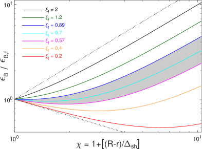
Figure 3: The evolution of the magnetic field equipartition parameter, $\epsilon_{B}$, with the distance behind the shock, according to Eq. (14). The value of $\epsilon_{B}$ normalized by that just after the shock is shown as a function of the Blandford & McKee (1976) self-similar variable $\chi=1+[(R-r)/\Delta_{\rm sh}]$ where $\Delta_{\rm sh}=R/[2(4-k)\Gamma_{\rm sh}^{2}]$, for several different values of the magnetic field anisotropy parameter just behind the shock, $\xi_{f}=0,\,0.2,\,0.4,\,0.57,\,0.7,\,0.89,\,1.2,\,2,\,\infty$ (from bottom to top). The two extreme values of $\xi_{f}=0,\,\infty$ are shown as dotted (straight) lines and correspond to power laws in $\chi$, as given in Eq. (14). The light-gray shaded region corresponds to the allowed range that we find in this work, $0.57\lesssim\xi_{f}\lesssim 0.89$.

5 Linear Polarization

To calculate the linear polarization averaged over the entire afterglow image on the plane of the sky, we start by first expressing the flux density measured by an off-axis observer whose LOS points in the direction of the unit vector $\hat{\textbf{{n}}}^{\prime}$ that makes an angle $\theta_{\rm obs}$ with the jet symmetry axis.

Here we consider synchrotron emission produced by relativistic electrons (or $e^{\pm}$-pairs) that are accelerated at the forward shock into a power law energy distribution, with $dN/d\gamma\propto\gamma^{-p}$ for $\gamma_{m}\leq\gamma\leq\gamma_{M}$. The comoving synchrotron emission coefficient (emitted energy per unit volume, time, frequency and solid angle) from a point-like region is given by

$$j^{\prime}_{\nu^{\prime}}=j^{\prime}_{\nu^{\prime},0}\nu^{\prime-\alpha}\langle[B(\theta_{B}^{\prime})\sin\delta^{\prime}]^{\epsilon}\rangle~{},$$ (15)

where it depends on the spectral index $\alpha$ and the component of the magnetic field perpendicular to the observer’s LOS, $B\sin\delta^{\prime}$, raised to some power $\epsilon=1+\alpha$ (Laing, 1980). Here $\delta^{\prime}$ is the angle between the local comoving magnetic field unit vector $\hat{\textbf{{B}}}$ and the direction to the observer, $\hat{\textbf{{n}}}^{\prime}\cdot\hat{\textbf{{B}}}=\cos\delta^{\prime}$, and it depends on the angle between the direction to the observer and the shock normal, given by $\tilde{\theta}^{\prime}=\arccos(\hat{\textbf{{n}}}^{\prime}\cdot\hat{\textbf{{n}}}_{\rm sh})$. The normalization, $j^{\prime}_{\nu^{\prime},0}=j^{\prime}_{\nu^{\prime},0}(\theta,y,R)$, depends on the energy density and number density of the radiating electrons (see, e.g., Gill & Granot, 2018). Since the magnetic field is tangled up in 3D with some anisotropy, the emissivity from a point-like region must be obtained by averaging over the different directions of the magnetic field, as indicated by the $\langle\rangle$ brackets, such that

$$\langle[B(\theta_{B}^{\prime})\sin\delta^{\prime}]^{\epsilon}\rangle=\frac{\int[B(\theta_{B}^{\prime})\sin\delta^{\prime}]^{\epsilon}f(\theta_{B}^{\prime})d\Omega_{B}^{\prime}}{\int f(\theta_{B}^{\prime})d\Omega_{B}^{\prime}}~{},$$ (16)

where the solid angle $d\Omega_{B}^{\prime}=\sin\theta_{B}^{\prime}d\theta_{B}^{\prime}d\varphi_{B}^{\prime}$ and $\varphi_{B}^{\prime}$ is the azimuthal angle. Since the magnetic field distribution is symmetric around $\hat{\textbf{{n}}}_{\rm sh}$, this average would depend only on the angle $\tilde{\theta}^{\prime}$ in addition to $\epsilon$ and $\xi$ (and these dependencies carry through to $j^{\prime}_{\nu^{\prime}}$). The flux density measured by an off-axis observer from a distant source at redshift $z$, corresponding to a luminosity distance $d_{L}$, is given by integrating over the volume of the emission region (e.g. Granot et al., 1999a),

$$F_{\nu}(t_{\rm obs},\theta_{\rm obs},\nu)=\frac{(1+z)}{d_{L}^{2}}\int_{0}^{2\pi}d\tilde{\varphi}\int_{-1}^{1}d\tilde{\mu}\int_{0}^{1}dy\left|\frac{dr}{dy}\right|\frac{(yR)^{2}j^{\prime}_{\nu^{\prime}}}{[\Gamma(1-\beta\tilde{\mu})]^{2}}\,,$$ (17)

where $\Gamma$ is the LF of the radiating fluid element, $\tilde{\mu}=\cos\tilde{\theta}=\hat{\textbf{{n}}}\cdot\hat{\bm{\beta}}=\hat{\textbf{{n}}}\cdot\hat{\textbf{{r}}}$, and $\tilde{\theta}$ and $\tilde{\varphi}$ are, respectively, the polar angle measured from and the azimuthal angle measured around the observer’s LOS.

Figure 4: Mapping between the two parameters, $b$ and $\xi_{f}$, that characterize the degree of anisotropy in the postshock magnetic field, shown at $t_{\rm obs}=244\,$days. This mapping is not constant in time. The $b=2\langle B_{\parallel}^{2}\rangle/\langle B_{\perp}^{2}\rangle$ parameter averages over both the radial profile and the local direction and strength distribution of the field and is used in 2D integrals of the emission region, which is assumed to be an infinitely thin shell. The $\xi_{f}$ parameter characterizes the anisotropy of the magnetic field just behind the shock and is used in 3D volume integrals of the emission region. The scaling of the local effective field anisotropy ($\xi_{\rm eff}$) with $b$ is also shown (also see the dotted lines in Fig 6).

The measured linear polarization ($V=0$) is obtained from the ratio of the polarized intensity to the total intensity, $\Pi=\sqrt{Q^{2}+U^{2}}/I$, where $I,Q,U,V$ are the Stokes parameters. Due to the assumed axisymmetry of the flow, $U$ vanishes, and the frequency independent polarization is therefore given by

$$\Pi(t_{\rm obs},\theta_{\rm obs})=\frac{Q}{I}=\frac{\int dF_{\nu}\cos(2\tilde{\varphi})\Pi^{\prime}}{\int dF_{\nu}}~{},$$ (18)

with $\Pi^{\prime}$ being the local polarization. When $\Pi<0$ ($\Pi>0$) the polarization vector on the plane of the sky is expected to be along (normal to) the direction of motion of the flux centroid. To obtain the local polarization $\Pi^{\prime}$ from a point-like region averaging over the different magnetic field directions is again performed, which yields (Sari, 1999)

$$\frac{\Pi^{\prime}}{\Pi_{\max}}=\frac{\int\cos(2\eta^{\prime})[B(\theta_{B}^{\prime})\sin\delta^{\prime}]^{\epsilon}f(\theta_{B}^{\prime})d\Omega_{B}^{\prime}}{\int[B(\theta_{B}^{\prime})\sin\delta^{\prime}]^{\epsilon}f(\theta_{B}^{\prime})d\Omega_{B}^{\prime}}~{},$$ (19)

where $\eta^{\prime}$ is the angle between the direction of the local polarization unit vector $\hat{\bm{\Pi}}^{\prime}=(\hat{\textbf{{n}}}^{\prime}\times\hat{\textbf{{B}}})/|\hat{\textbf{{n}}}^{\prime}\times\hat{\textbf{{B}}}|$ and the direction perpendicular to the plane containing $\hat{\textbf{{n}}}^{\prime}$ and $\hat{\bm{\beta}}$. When $\Pi^{\prime}>0$ ($\Pi^{\prime}<0$) the direction of the local polarization vector is along (normal to) the direction of $\hat{\textbf{{n}}}\times\hat{\textbf{{n}}}_{\rm sh}$. Again, because of the magnetic field’s symmetry around $\hat{\textbf{{n}}}_{\rm sh}$, this ratio depends only on $\tilde{\theta}^{\prime}$, $\epsilon$ and $\xi$. For $\epsilon=2$ (with $\alpha=1$), the expression for the polarization becomes particularly simple, and Eq. (19) yields (Gruzinov, 1999; Sari, 1999)

$$\frac{\Pi^{\prime}(\tilde{\theta}^{\prime})}{\Pi_{\max}}=\frac{(b-1)\sin^{2}\tilde{\theta}^{\prime}}{2+(b-1)\sin^{2}\tilde{\theta}^{\prime}}\quad\quad\quad(\epsilon=2)~{},$$ (20)

where $\cos\tilde{\theta}^{\prime}\equiv\tilde{\mu}^{\prime}=(\tilde{\mu}-\beta)/(1-\beta\tilde{\mu})$. Here $b\equiv 2\langle B_{\parallel}^{2}\rangle/\langle B_{\perp}^{2}\rangle$ is another way to parameterize the anisotropy of the magnetic field (Granot & Königl, 2003), where the average is taken over the radial profile of the flow downstream of the shock and the local direction and strength distribution of the magnetic field. This choice of parameterization is most useful when considering emission from an infinitely thin region behind the shock (see, e.g., Granot & Königl, 2003), for which the degree of polarization is obtained from

$$\Pi_{\rm 2D}=\frac{Q}{I}=\frac{\int\delta_{D}^{3}L^{\prime}_{\nu^{\prime}}\langle[B(\theta_{B}^{\prime})\sin\delta^{\prime}]^{2}\rangle\Pi^{\prime}\cos(2\tilde{\varphi})d\tilde{\Omega}}{\int\delta_{D}^{3}L^{\prime}_{\nu^{\prime}}\langle[B(\theta_{B}^{\prime})\sin\delta^{\prime}]^{2}\rangle d\tilde{\Omega}}\quad(\epsilon=2)~{},$$ (21)

where $d\tilde{\Omega}=d\tilde{\mu}d\tilde{\varphi}$ and $L^{\prime}_{\nu^{\prime}}$ is the isotropic equivalent (locally anisotropic) synchrotron spectral power (see Gill & Granot, 2018, for further details). Averaging over different magnetic field directions follows from Eq. (16), which yields

$$\langle[B(\theta_{B}^{\prime})\sin\delta^{\prime}]^{2}\rangle\propto 2+(b-1)\sin^{2}\tilde{\theta}^{\prime}\quad\quad\quad(\epsilon=2)~{}.$$ (22)

In Fig. 4 we show the mapping between $b$ and $\xi_{f}$ that was obtained by comparing the degree of polarization in the two cases for the two different jet structures at $t_{\rm obs}=244\,$days. Note that applying the local definition of $b$ to our local magnetic field model that is defined by $\xi$ alone yields the simple relation $b\equiv 2\langle B_{\parallel}^{2}\rangle/\langle B_{\perp}^{2}\rangle=\xi^{2}$ (see appendix (A)). This local relation largely carries through to the global mapping between $b$ and $\xi_{f}$ shown in Fig. 4, when accounting for the fact that since $\xi$ increases with the distance behind the shock, its effective value that can be defined as $\xi_{\rm eff}=b^{1/2}$ is somewhat higher than that just behind the shock ($\xi_{f}$).

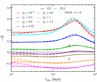
Figure 5: Temporal evolution of the degree of linear polarization ($\Pi$), obtained from a volume integration of the flow, shown for different values of the magnetic field anisotropy parameter, $\xi_{f}$, just behind the shock. The two arrows mark the polarization upper limit, $|\Pi|<12\%$. Comparison is made between two jet structures – a gaussian jet (GJ) and a power law jet (PLJ). The result from Gill & Granot (2018, GG18), which assumed an infinitely thin shell geometry as well as locally isotropic synchrotron spectral emissivity (see footnote 2), is also shown for the magnetic field anisotropy parameter $b=0$. The jet and afterglow model parameters are the same as assumed in GG18.

We present the temporal evolution of the linear polarization for different $\xi_{f}$ parameter values and the two jet structures in Fig. 5. The polarization curve obtained from the 2D surface integral for $b=0$ in GG18 is also shown for comparison. As shown in GG18, the peak of the polarization occurs at $\sim 2t_{\rm obs,pk}$, where $t_{\rm obs,pk}\approx 150\,$days is the peak of the lightcurve when the compact relativistic core of the outflow becomes visible to the off-axis observer. This remains true for $\xi_{f}<1$. As the two parameters are increased above zero the degree of anisotropy of the magnetic field begins to decline, until the field becomes completely isotropic, which occurs at $b=1$ and $\xi_{f}\approx 0.72$ (corresponding to $\xi_{\rm eff}=1$) in the two cases. This also marks the point when the polarization vanishes and the polarization position angle undergoes a $90^{\circ}$ flip. Prior to this point, as the magnetic field anisotropy decreases the level of polarization also declines. The trend reverses post this point, when the $B_{\parallel}$ components starts to dominate over the $B_{\perp}$ component and as the field again becomes increasingly anisotropic.

An upper limit on the degree of linear polarization of $|\Pi|<12\%$ ($99\%$ confidence) was measured by Corsi et al. (2018) from the radio afterglow of GW 170817 / GRB 170817A  using the VLA at $t_{\rm obs}\approx 244\,$days and $\nu=2.8\;$GHz. Since the polarization angle could not be constrained, the upper limit, shown as two black arrows in Fig. 5, constrains the absolute value of the true degree of polarization. We use this upper limit to constrain the value of both $0.66\lesssim b\lesssim 1.49$ and $0.57\lesssim\xi_{f}\lesssim 0.89$ in Fig. 6, where we show the degree of polarization at $t_{\rm obs}=244\,$days as a function of $b$ and $\xi_{f}$ for the two jet structures. The postshock field anisotropy ($\xi_{f}$) may have some dependence on the shock compression ratio, $\rho_{f}/\rho_{k}(r)=2^{3/2}\Gamma_{\rm sh}=4\Gamma_{f}$ (see Eq. (7); where the last equality is true when $\Gamma_{\rm sh}\gg 1$). The corresponding ranges for the flux-weighted mean of the two LFs and for the two jet structures are: (GJ) $4.26\leq\langle\Gamma_{\rm sh}\rangle\leq 4.59$; $3.31\leq\langle\Gamma_{f}\rangle\leq 3.59$, (PLJ) $3.98\leq\langle\Gamma_{\rm sh}\rangle\leq 4.24$; $3.10\leq\langle\Gamma_{f}\rangle\leq 3.30$. The dotted lines in Fig. 5 show $\Pi(\xi_{f}^{2})$ that have the same trend as $\Pi(b)$. This similarity results from the local scaling (averaged over the field’s angular distribution) where $b=\xi^{2}$. It is preserved in the global 3D integration where the effective anisotropy of the postshock field scales as $\xi_{\rm eff}=b^{1/2}$.

6 Discussion

The upper limit of $|\Pi|<12\%$ measured for the afterglow linear polarization for GW 170817 / GRB 170817A  has important implications for the postshock magnetic field structure, in particular for its degree of anisotropy. In the case of Weibel instability-generated magnetic fields just behind the forward shock, the theoretically expected value (e.g., Medvedev & Loeb, 1999) of the anisotropy parameter is $\xi_{f}=0$ (corresponding to $b=0$ in the 2D case). As shown in Fig. 6, this case is ruled out and the constrained value of $0.57\lesssim\xi_{f}\lesssim 0.89$ suggests that the magnetic field just behind the shock must have a finite but sub-dominant $B_{\parallel}$ component. In terms of the parameter $b$, which is more suitable for a 2D thin emitting shell, we obtain $0.66\lesssim b\lesssim 1.49$. This is a significant improvement compared to the previous rough estimate of $0.5\lesssim b\lesssim 2$ made by Granot & Königl (2003) based on the low measured values ($\Pi\lesssim\;$few % in the optical/NIR) of afterglow linear polarization in the first several GRB afterglows (which were available at that time), which involved a statistical argument since the jet angular structure and $\theta_{\rm obs}$ were not known for those GRBs.

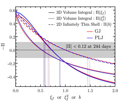
Figure 6: Linear polarization ($\Pi$) as a function of the magnetic field anisotropy parameter just behind the shock $\xi_{f}$ for a 3D volume integral or the anisotropy paremeter $b$ for a 2D infinitely thin shell (Gill & Granot, 2018). The upper limit on $|\Pi|$ measured by Corsi et al. (2018) at $t_{\rm obs}\approx 244\,$days post merger is shown as the gray shaded region. This constrains $0.57\lesssim\xi_{f}\lesssim 0.89$ and $0.66\lesssim b\lesssim 1.49$ for both the Gaussian jet (GJ; $0.57\lesssim\xi_{f}\lesssim 0.89$, $0.66\lesssim b\lesssim 1.49$) and power law jet (PLJ; $0.59\lesssim\xi_{f}\lesssim 0.89$, $0.68\lesssim b\lesssim 1.46$). The dotted lines show $\Pi(\xi_{f}^{2})$ having the same shape as $\Pi(b)$ demonstrating that, since locally $b=\xi^{2}$, a global 3D integration preserves the same scaling for an effective anisotropy parameter, $\xi_{\rm eff}=b^{1/2}$.

On the other hand, 3D PIC simulations of two counterstreaming unmagnetized relativistic electron-ion (or even electron-positron) plasmas find that the magnetic field just behind the shock is predominantly transverse, with a finite component parallel to the shock normal having, on average, $|B_{\parallel}|/|B|\lesssim 10^{-2}$ (e.g., Frederiksen et al., 2004; Ardaneh et al., 2015; Ardaneh et al., 2016). Expressing this ratio in terms of the anisotropy parameter, we find $|B_{\parallel,f}|/|B_{f}|=\xi_{f}(1+\xi_{f}^{2})^{-1/2}\simeq 0.50-0.66$ for $0.57\lesssim\xi_{f}\lesssim 0.89$, which suggests that the field anisotropy just behind the shock is significantly smaller as compared to that found in those PIC simulations. Furthermore, due to the larger stretching of the flow in the radial direction (compared to the two transverse directions) $|B_{\parallel,f}|/|B_{f}|$ grows with the distance behind the shock (however this occurs on the dynamical scales where the planar symmetry of the PIC simulations breaks down and the shock’s radius of curvature becomes important). Since PIC simulations are generally limited to box-sizes that span at most $\lesssim 10^{4}(c/\omega_{p,e})$ (see, e.g., Spitkovsky, 2008a; Keshet et al., 2009, for 2D simulations), which is still much smaller than the width of the postshock region, the decline in field anisotropy over larger scales remains unconstrained.

In modeling the afterglow, we have explicitly made the assumption that $\epsilon_{B}$ (with $\epsilon_{B,f}=5.5\times 10^{-4}$ in this work, though it is still subject to degeneracies with other model parameters, e.g. Gill et al. 2019) depends on the radial profile of the flow in the shocked region. PIC simulations show that the two-stream/Weibel instability amplifies the magnitude of small scale shock-generated magnetic field to near-equipartition ($\epsilon_{B}\sim 0.1$) in the shock transition region that separates the upstream and downstream flows. However, many 2D PIC simulations find that due to particle phase-space mixing the field decays rapidly downstream within few $\times\,100(c/\omega_{p,e})$ (e.g., Kato, 2007; Chang et al., 2008; Spitkovsky, 2008a). The long-term evolution of both electron-ion (Takamoto et al., 2018) and $e^{\pm}$-pair plasma (Keshet et al., 2009) PIC simulations does seem to suggest that the magnetic field decay saturates at $\epsilon_{B}\sim 10^{-2}$ for comoving distances $\gtrsim 10^{2}(c/\omega_{p,e})$ from the shock transition region. However, due to the small dynamical scales probed in these simulations and the assumption of planar symmetry, the radial stretching of fluid elements is not observed. Therefore, a self-consistent treatment assuming flux freezing once plasma effects saturate and $\xi_{f}$ with the corresponding $\epsilon_{B,f}$ is established, would require $\epsilon_{B}$ to evolve with $\chi$ according to Eq. (14).

Early 2D PIC simulations that showed a gradual power law decay of $\epsilon_{B}$ prompted the consideration of decaying magnetic fields in the bulk of the shocked region for afterglow modeling (Rossi & Rees, 2003; Lemoine et al., 2013; Lemoine, 2015) and also in models of prompt emission from internal shocks (Pe’er & Zhang, 2006; Derishev, 2007). Moreover, afterglow modeling of many GRBs in the optical band revealed a wide distribution with a rather low value of the radially averaged magnetic field in the shocked region with $10^{-8}\lesssim\langle\epsilon_{B}\rangle\lesssim 10^{-2}$ under the explicit assumption that the circumburst density $n=1\,{\rm cm}^{-3}$ (Santana et al., 2014). Therefore, even though long-term PIC simulations might hint at saturation of the field, as mentioned above, more realistic simulations for the GRB afterglow shock should show its evolution with $\xi$ in the downstream.

Instead of generating magnetic field in the shock upstream via microscopic plasma instabilities (e.g., two-stream/Weibel), it has been argued (Sironi & Goodman, 2007; Couch et al., 2008; Goodman & MacFadyen, 2008) and demonstrated using MHD simulations (Zhang et al., 2009; Inoue et al., 2011; Mizuno et al., 2011) that macroscopic turbulence can amplify the feeble ($\epsilon_{B}\sim 10^{-9}$) ISM magnetic field to $\epsilon_{B}\sim\Gamma^{-1}\gtrsim 10^{-2}$, with $\Gamma\lesssim{\rm few}\times 10^{2}$ for GRB afterglows, via vorticity generation at the shock transition due to density inhomogeneities in the shock upstream. As the cold density clumps pass through the shock transition, vortical eddies are created in the downstream that twist and stretch the seed magnetic field. This leads to amplification of the field strength over the eddy turn-over time due to the dynamo mechanism. The density clumps in the upstream can arise either from preexisting density inhomogeneities in the stellar wind (relevant only to long-soft GRBs) or can be self-generated due to partial charge separation between the shock accelerated non-thermal ions and electrons in the upstream (Couch et al., 2008). The advantage of turbulence amplified magnetic field is that its coherence length is much larger than plasma skin-depth scales, making it less susceptible to decay due to particle phase space mixing. Moreover, the postshock field tends to be more isotropic, which is consistent with the findings of this work.

7 Conclusions

In this work, we have used the upper limit on the linear polarization, $|\Pi|<12\%$ at $t_{\rm obs}\approx 244\,$ days, of the radio afterglow of GW 170817 / GRB 170817A  to constrain the anisotropy of the shock-generated tangled magnetic field. The structure of the outflow was modeled using the best-fit solution (from afterglow data up to $t_{\rm obs}\sim 600\,$days) obtained in Gill & Granot (2018); Gill et al. (2019) for a Gaussian and a power-law jet with locally spherical dynamics and no sideways spreading. Since the flux at the time of polarization measurement was dominated by the relativistic core, with $\Gamma(t_{\rm obs}=244\,{\rm days})\approx 4.1(t_{\rm obs}/150\,{\rm days})^{-3/8}=3.4$, the assumption of no sideways spreading, which is important when the flow becomes non-relativistic (e.g., van Eerten & MacFadyen, 2012), should still remain reasonably valid. As suggested by the broadband (X-ray/Optical/Radio) afterglow synchrotron emission, which maintained a single power law with $\nu_{m}<\nu<\nu_{c}$, the shock-heated relativistic power-law electrons were slow cooling. This necessitated the need for integrating over the entire shocked volume, rather than assuming an infinitely thin emission region behind the shock, to calculate the observed linear polarization. In order to do that, we have modeled the radial profile of the postshock magnetic field using the BM76 relativistic spherical self-similar solution. Under the frozen-field approximation, this causes the magnetic field to become increasingly radial since the farther downstream the flow is the more radially (as compared to the transverse direction) stretched a given fluid element becomes.

Our main conclusion is that the shock-generated tangled magnetic field cannot lie only in the plane of the shock (perpendicular to the shock normal, $B_{\perp}$), as posited by some theoretical works (e.g., Medvedev & Loeb, 1999) and also shown in some PIC simulations (e.g., Chang et al., 2008). We find that the field just behind the shock must have a finite, albeit mildly sub-dominant, component parallel to the shock normal, $B_{\parallel}$, which is radial in our case. Moreover, the initial field anisotropy parameter must be in the range $0.57\lesssim(\xi_{f}=B_{\parallel,f}/B_{\perp,f})\lesssim 0.89$, and $\xi=B_{\parallel}/B_{\perp}=\xi_{f}\chi^{(7-2k)/(8-2k)}$ grows downstream with the distance behind the shock. This presents a mismatch between our results and that obtained both from analytic arguments and current PIC simulations of relativistic collisionless shocks, suggesting that larger scale and long-term simulations are needed to better constrain the asymptotic structure of the postshock magnetic field. At the same time, the lower degree of polarization of afterglow emission that reflects the inherent higher level of isotropy of the postshock magnetic field may be consistent with turbulence amplified magnetic field.

Appendix A Magnetic field evolution as it is advected downstream of the shock

Here we derive the evolution of the magnetic field as it is advected downstream of the shock, assuming a local (i.e. at each given angle $\theta$ from the jet symmetry axis) Blandford & McKee (1976) radial dynamics. Let a subscript “0” denote the value of a quantity when the fluid element that is currently (at a local shock radius $R$) at $\chi=1+2(4-k)\Gamma_{\rm sh}^{2}(R)[(R-r)/R]$, just crossed the shock (and was at $\chi=1$ when the shock radius was $R_{0}$), while a subscript “$f$” denotes the current (at a shock radius $R$) value of a quantity just behind the shock (at $\chi=1$). We have (Granot et al., 1999a; Granot & Sari, 2002) $\chi=(R/R_{0})^{4-k}$ while the proper internal energy density scales as

$$\frac{e}{e_{0}}=\chi^{-\frac{2(13-2k)}{3(4-k)}}\ ,\quad\quad\frac{e_{f}}{e_{0}}=\chi^{-\frac{3}{4-k}}\ .$$ (23)

The comoving length of a fluid element in the direction parallel to the shock normal $\hat{\textbf{{n}}}_{\rm sh}$ and the two directions perpendicular to it scale as (Granot et al., 1999a; Granot & Königl, 2003)

$$\frac{L_{\parallel}}{L_{\parallel,0}}=\chi^{\frac{9-2k}{2(4-k)}}\ ,\quad\quad\frac{L_{\perp}}{L_{\perp,0}}=\frac{R}{R_{0}}=\chi^{\frac{1}{4-k}}\ .$$ (24)

Assuming flux freezing as the fluid element is advected downstream, the two corresponding components of the comoving magnetic field scale as

$$\frac{B_{\parallel}}{B_{\parallel,0}}=\frac{L_{\perp,0}^{2}}{L_{\perp}^{2}}=\chi^{-\frac{2}{4-k}}\ ,\quad\quad\frac{B_{\perp}}{B_{\perp,0}}=\frac{L_{\perp,0}L_{\parallel,0}}{L_{\perp}L_{\parallel}}=\chi^{-\frac{11-2k}{2(4-k)}}\ .$$ (25)

Now, in order to calculate the evolution of $\epsilon_{B}=\langle{B^{2}}\rangle/8\pi e$ we need to calculate the mean of the square of the magnetic field. In our formalism the magnetic field is derived from an isotropic distribution that we will denote by a bar, with constant magnetic field strength $\bar{B}$ and angular probability density $\bar{f}=1/4\pi$ so that $\int\bar{f}d\bar{\Omega}^{\prime}_{B}=1$ where $d\bar{\Omega}^{\prime}_{B}=d\bar{\varphi}^{\prime}_{B}d\bar{\mu}$ and $\bar{\mu}=\cos\bar{\theta}^{\prime}_{B}$. Since the field is symmetric with respect to $\hat{\textbf{{n}}}_{\rm sh}$, i.e. $\bar{f}=f(\hat{\theta}^{\prime}_{B})$, then we can integrate over $\bar{\varphi}^{\prime}_{B}$ and switch from $\bar{f}d\bar{\Omega}^{\prime}_{B}$ to $\bar{f}_{\mu}d\bar{\mu}$ where $\bar{f}_{\mu}=\frac{1}{2}$ is normalized such that $\int_{-1}^{1}\bar{f}_{\mu}d\bar{\mu}=1$. The magnetic field is derived from this distribution by stretching the component parallel to $\hat{\textbf{{n}}}_{\rm sh}$ by a factor $\xi$ while the perpendicular component remains unchanged,

$$\xi=\frac{B_{\parallel}}{\bar{B}_{\parallel}}=\frac{B\mu}{\bar{B}\bar{\mu}}\ ,\quad\quad 1=\frac{B_{\perp}}{\bar{B}_{\perp}}=\frac{B}{\bar{B}}\sqrt{\frac{1-\mu^{2}}{1-\bar{\mu}^{2}}}\ .$$ (26)

This implies the relation

$$\bar{\mu}=\left[1+\xi^{2}(\mu^{-2}-1)\right]^{-1/2}\ ,$$ (27)

and therefore the post-stretching magnetic field strength as a function of $\mu=\cos\theta^{\prime}_{B}=\hat{\textbf{{n}}}_{\rm sh}\cdot\hat{\textbf{{B}}}$ is

$$\frac{B}{\bar{B}}=\sqrt{\frac{B_{\parallel}^{2}+B_{\perp}^{2}}{\bar{B}^{2}}}=\frac{\xi}{\sqrt{\xi^{2}(1-\mu^{2})+\mu^{2}}}\ .$$ (28)

The implied post-stretching angular probability distribution is

$$f_{\mu}(\mu)=\bar{f}_{\mu}\frac{d\bar{\mu}}{d\mu}=\frac{\xi^{2}}{2}\left(\frac{\bar{\mu}}{\mu}\right)^{3}=\frac{1}{2\xi}\left(\frac{B}{\bar{B}}\right)^{3}=\frac{\frac{1}{2}\xi^{2}}{\left[\xi^{2}(1-\mu^{2})+\mu^{2}\right]^{3/2}}\ .$$ (29)

Now it is straightforward to calculate the mean of any quantity $Q$ over the magnetic field as $\langle{Q}\rangle=\int_{-1}^{1}d\mu f_{\mu}(\mu)\,Q$. Note that more generally, when $Q$ also depends on $\varphi=\varphi^{\prime}_{B}$, one needs to evaluate $\langle{Q}\rangle=\int_{0}^{2\pi}d\varphi\int_{-1}^{1}d\mu f(\mu)\,Q(\mu,\varphi)$ where $f(\mu)=f_{\mu}(\mu)/2\pi$. In particular, the mean of the square of the parallel and perpendicular field components, normalized by their post-stretching values, are

$$\frac{\langle{B_{\parallel}^{2}}\rangle}{\langle{\bar{B}^{2}}\rangle}=\frac{\xi^{2}}{3}\ ,\quad\quad\frac{\langle{B_{\perp}^{2}}\rangle}{\langle{\bar{B}^{2}}\rangle}=\frac{2}{3}\ ,\quad\quad\frac{\langle{B^{2}}\rangle}{\langle{\bar{B}^{2}}\rangle}=\frac{\langle{B_{\perp}^{2}}\rangle+\langle{B_{\parallel}^{2}}\rangle}{\langle{\bar{B}^{2}}\rangle}=\frac{2+\xi^{2}}{3}\ .$$ (30)

This result can be understood in a simple way. Before the stretching the field is isotropic so each of the three directions holds $\frac{1}{3}$ of $\langle{\bar{B}^{2}}\rangle=\bar{B}^{2}$, and since there are two perpendicular directions and one parallel direction then $\langle{\bar{B}_{\perp}^{2}}\rangle=\frac{2}{3}\langle{\bar{B}^{2}}\rangle$ and $\langle{\bar{B}_{\parallel}^{2}}\rangle=\frac{1}{3}\langle{\bar{B}^{2}}\rangle$. Since the perpendicular component remains unchanged ($B_{\perp}=\bar{B}_{\perp}$) so does the mean of its square, and since the parallel component changes by a factor of $\xi$ then its square changes by a factor of $\xi^{2}$ everywhere, and so does its mean value. This result immediately gives us the local value of the parameter $b$,

$$b\equiv\frac{2\langle{B_{\parallel}^{2}}\rangle}{\langle{B_{\perp}^{2}}\rangle}=\xi^{2}\ ,\quad\quad b(\,\chi)=\xi^{2}(\,\chi)=\xi_{f}^{2}\,\chi^{\frac{7-2k}{4-k}}\ .$$ (31)

In our formalism, the local pre-stretching magnetic field strength corresponds to $\bar{B}\to B_{\perp,\rm{max}}=B(\mu=0)$. According to Eq. (25), $B_{\perp,\rm{max}}^{2}/B_{\perp,\rm{max},0}^{2}=\chi^{-(11-2k)/(4-k)}$, and therefore

$$\frac{\langle{B^{2}}\rangle}{\langle{B_{0}^{2}}\rangle}=\frac{2+\xi^{2}}{2+\xi_{0}^{2}}\frac{B_{\perp,\rm{max}}^{2}}{B_{\perp,\rm{max},0}^{2}}=\frac{2+\xi_{f}^{2}\,\chi^{\frac{7-2k}{4-k}}}{2+\xi_{f}^{2}}\,\chi^{-\frac{11-2k}{4-k}}\ .$$ (32)

We assume here for simplicity that both $\xi$ and $\epsilon_{B}$ have a universal value just behind the shock (at $\chi=1$), so that $\xi_{0}\equiv\xi(R_{0},\chi=1)=\xi(R,\chi=1)\equiv\xi_{f}$ and $\epsilon_{B,0}\equiv\epsilon_{B}(R_{0},\chi=1)=\epsilon_{B}(R,\chi=1)\equiv\epsilon_{B,f}$. This in not obvious since $\epsilon_{B,f}$ may vary with $\Gamma_{\rm sh}$ in the mildly relativistic regime, while $\xi_{f}$ may even vary in the ultra-relativistic regime, if e.g. it depends on the shock compression ratio. Anyway, under our assumptions, using Eqs. (23) and (32) the evolution of $\epsilon_{B}$ is given by

$$\frac{\epsilon_{B}}{\epsilon_{B,f}}=\frac{\epsilon_{B}}{\epsilon_{B,0}}=\frac{\langle{B^{2}}\rangle}{\langle{B_{0}^{2}}\rangle}\frac{e_{0}}{e}=\frac{2+\xi_{f}^{2}\,\chi^{\frac{7-2k}{4-k}}}{\left(2+\xi_{f}^{2}\right)\,\chi^{\frac{7-2k}{3(4-k)}}}\ .$$ (33)

Similarly, the magnetic field just behind the shock is given by $B_{\perp,\rm{max},f}^{2}/B_{\perp,\rm{max},0}^{2}=\epsilon_{B,f}e_{f}/\epsilon_{B,0}e_{0}=e_{f}/e_{0}=\chi^{-\frac{3}{4-k}}$, so that

$$\frac{B_{\perp,\rm{max}}}{B_{\perp,\rm{max},f}}=\frac{B_{\perp,\rm{max}}}{B_{\perp,\rm{max},0}}\frac{B_{\perp,\rm{max},0}}{B_{\perp,\rm{max},f}}=\chi^{-1}\ ,$$ (34)

$$\frac{\langle{B_{\parallel}^{2}}\rangle}{\langle{B_{f}^{2}}\rangle}=\frac{\xi^{2}\chi^{-2}}{2+\xi_{f}^{2}}=\frac{\xi_{f}^{2}}{2+\xi_{f}^{2}}\,\chi^{-\frac{1}{4-k}}\ ,\quad\quad\frac{\langle{B_{\perp}^{2}}\rangle}{\langle{B_{f}^{2}}\rangle}=\frac{2\,\chi^{-2}}{2+\xi_{f}^{2}}\ .$$ (35)

$$\frac{\langle{B^{2}}\rangle}{\langle{B_{f}^{2}}\rangle}=\frac{2+\xi^{2}}{2+\xi_{f}^{2}}\,\chi^{-2}=\frac{2+\xi_{f}^{2}\,\chi^{\frac{7-2k}{4-k}}}{(2+\xi_{f}^{2})\,\chi^{2}}\ .$$ (36)

References

- Abbott et al. (2017a) Abbott B. P., et al., 2017a, Physical Review Letters, 119, 161101
- Abbott et al. (2017b) Abbott B. P., et al., 2017b, ApJ, 848, L13
- Alexander et al. (2018) Alexander K. D., et al., 2018, ApJ, 863, L18
- Ardaneh et al. (2015) Ardaneh K., Cai D., Nishikawa K.-I., Lembége B., 2015, ApJ, 811, 57
- Ardaneh et al. (2016) Ardaneh K., Cai D., Nishikawa K.-I., 2016, ApJ, 827, 124
- Blandford & McKee (1976) Blandford R. D., McKee C. F., 1976, Physics of Fluids, 19, 1130
- Bret (2009) Bret A., 2009, ApJ, 699, 990
- Chang et al. (2008) Chang P., Spitkovsky A., Arons J., 2008, ApJ, 674, 378
- Corsi et al. (2018) Corsi A., et al., 2018, ApJ, 861, L10
- Couch et al. (2008) Couch S. M., Milosavljević M., Nakar E., 2008, ApJ, 688, 462
- Covino & Gotz (2016) Covino S., Gotz D., 2016, Astronomical and Astrophysical Transactions, 29, 205
- Covino et al. (1999) Covino S., et al., 1999, A&A, 348, L1
- D’Avanzo et al. (2018) D’Avanzo P., et al., 2018, A&A, 613, L1
- De Colle et al. (2012) De Colle F., Granot J., López-Cámara D., Ramirez-Ruiz E., 2012, ApJ, 746, 122
- Derishev (2007) Derishev E. V., 2007, Ap&SS, 309, 157
- Frederiksen et al. (2004) Frederiksen J. T., Hededal C. B., Haugbølle T., Nordlund Å., 2004, ApJ, 608, L13
- Ghirlanda et al. (2019) Ghirlanda G., et al., 2019, Science
- Ghisellini & Lazzati (1999) Ghisellini G., Lazzati D., 1999, MNRAS, 309, L7
- Gill & Granot (2018) Gill R., Granot J., 2018, MNRAS, 478, 4128
- Gill et al. (2018) Gill R., Granot J., Kumar P., 2018, arXiv e-prints, p. arXiv:1811.11555
- Gill et al. (2019) Gill R., Granot J., De Colle F., Urrutia G., 2019, arXiv:1902.10303, e-prints,
- Goodman & MacFadyen (2008) Goodman J., MacFadyen A., 2008, Journal of Fluid Mechanics, 604, 325
- Granot & Königl (2003) Granot J., Königl A., 2003, ApJ, 594, L83
- Granot & Sari (2002) Granot J., Sari R., 2002, ApJ, 568, 820
- Granot et al. (1999a) Granot J., Piran T., Sari R., 1999a, ApJ, 513, 679
- Granot et al. (1999b) Granot J., Piran T., Sari R., 1999b, ApJ, 527, 236
- Gruzinov (1999) Gruzinov A., 1999, ApJ, 525, L29
- Gruzinov (2001) Gruzinov A., 2001, ApJ, 563, L15
- Gruzinov & Waxman (1999) Gruzinov A., Waxman E., 1999, ApJ, 511, 852
- Hajela et al. (2019) Hajela A., et al., 2019, arXiv e-prints, p. arXiv:1909.06393
- Hallinan et al. (2017) Hallinan G., et al., 2017, Science, 358, 1579
- Inoue et al. (2011) Inoue T., Asano K., Ioka K., 2011, ApJ, 734, 77
- Ioka & Nakamura (2001) Ioka K., Nakamura T., 2001, ApJ, 554, L163
- Kato (2007) Kato T. N., 2007, ApJ, 668, 974
- Keshet et al. (2009) Keshet U., Katz B., Spitkovsky A., Waxman E., 2009, ApJ, 693, L127
- Kumar & Granot (2003) Kumar P., Granot J., 2003, ApJ, 591, 1075
- Kumar & Piran (2000) Kumar P., Piran T., 2000, ApJ, 535, 152
- Kumar & Zhang (2015) Kumar P., Zhang B., 2015, Phys. Rep., 561, 1
- Laing (1980) Laing R. A., 1980, MNRAS, 193, 439
- Lamb & Kobayashi (2018) Lamb G. P., Kobayashi S., 2018, MNRAS, 478, 733
- Lamb et al. (2019) Lamb G. P., et al., 2019, ApJ, 870, L15
- Laskar et al. (2019) Laskar T., et al., 2019, ApJ, 878, L26
- Lazzati et al. (2018) Lazzati D., Perna R., Morsony B. J., Lopez-Camara D., Cantiello M., Ciolfi R., Giacomazzo B., Workman J. C., 2018, Physical Review Letters, 120, 241103
- Lemoine (2015) Lemoine M., 2015, Journal of Plasma Physics, 81, 455810101
- Lemoine et al. (2013) Lemoine M., Li Z., Wang X.-Y., 2013, MNRAS, 435, 3009
- Loeb & Perna (1998) Loeb A., Perna R., 1998, ApJ, 495, 597
- Lyman et al. (2018) Lyman J. D., et al., 2018, Nature Astronomy, 2, 751
- Margutti et al. (2018) Margutti R., et al., 2018, ApJ, 856, L18
- Medvedev & Loeb (1999) Medvedev M. V., Loeb A., 1999, ApJ, 526, 697
- Medvedev et al. (2005) Medvedev M. V., Fiore M., Fonseca R. A., Silva L. O., Mori W. B., 2005, ApJ, 618, L75
- Mészáros & Rees (1997) Mészáros P., Rees M. J., 1997, ApJ, 476, 232
- Mészáros et al. (1998) Mészáros P., Rees M. J., Wijers R. A. M. J., 1998, ApJ, 499, 301
- Milosavljević & Nakar (2006) Milosavljević M., Nakar E., 2006, ApJ, 641, 978
- Mizuno et al. (2011) Mizuno Y., Pohl M., Niemiec J., Zhang B., Nishikawa K.-I., Hardee P. E., 2011, ApJ, 726, 62
- Moiseev & Sagdeev (1963) Moiseev S. S., Sagdeev R. Z., 1963, Journal of Nuclear Energy, 5, 43
- Mooley et al. (2018a) Mooley K. P., et al., 2018a, Nature, 554, 207
- Mooley et al. (2018b) Mooley K. P., et al., 2018b, Nature, 561, 355
- Nakar & Oren (2004) Nakar E., Oren Y., 2004, ApJ, 602, L97
- Nakar et al. (2011) Nakar E., Bret A., Milosavljević M., 2011, ApJ, 738, 93
- Nynka et al. (2018) Nynka M., Ruan J. J., Haggard D., Evans P. A., 2018, ApJ, 862, L19
- Panaitescu & Kumar (2000) Panaitescu A., Kumar P., 2000, ApJ, 543, 66
- Panaitescu & Kumar (2002) Panaitescu A., Kumar P., 2002, ApJ, 571, 779
- Pe’er & Zhang (2006) Pe’er A., Zhang B., 2006, ApJ, 653, 454
- Piran (2004) Piran T., 2004, Reviews of Modern Physics, 76, 1143
- Piran (2005) Piran T., 2005, in de Gouveia dal Pino E. M., Lugones G., Lazarian A., eds, American Institute of Physics Conference Series Vol. 784, Magnetic Fields in the Universe: From Laboratory and Stars to Primordial Structures.. pp 164–174 (arXiv:astro-ph/0503060), doi:10.1063/1.2077181
- Resmi et al. (2018) Resmi L., et al., 2018, ApJ, 867, 57
- Rossi & Rees (2003) Rossi E., Rees M. J., 2003, MNRAS, 339, 881
- Rossi et al. (2004) Rossi E. M., Lazzati D., Salmonson J. D., Ghisellini G., 2004, MNRAS, 354, 86
- Santana et al. (2014) Santana R., Barniol Duran R., Kumar P., 2014, ApJ, 785, 29
- Sari (1999) Sari R., 1999, ApJ, 524, L43
- Sari et al. (1998) Sari R., Piran T., Narayan R., 1998, ApJ, 497, L17
- Silva et al. (2003) Silva L. O., Fonseca R. A., Tonge J. W., Dawson J. M., Mori W. B., Medvedev M. V., 2003, ApJ, 596, L121
- Sironi & Goodman (2007) Sironi L., Goodman J., 2007, ApJ, 671, 1858
- Sironi et al. (2015) Sironi L., Keshet U., Lemoine M., 2015, Space Sci. Rev., 191, 519
- Spitkovsky (2008a) Spitkovsky A., 2008a, ApJ, 673, L39
- Spitkovsky (2008b) Spitkovsky A., 2008b, ApJ, 673, L39
- Takamoto et al. (2018) Takamoto M., Matsumoto Y., Kato T. N., 2018, ApJ, 860, L1
- Troja et al. (2017) Troja E., et al., 2017, Nature, 551, 71
- Troja et al. (2018) Troja E., et al., 2018, MNRAS, 478, L18
- Waxman (1997) Waxman E., 1997, ApJ, 485, L5
- Weibel (1959) Weibel E. S., 1959, Phys. Rev. Lett., 2, 83
- Wijers & Galama (1999) Wijers R. A. M. J., Galama T. J., 1999, ApJ, 523, 177
- Wijers et al. (1999) Wijers R. A. M. J., et al., 1999, ApJ, 523, L33
- Yamazaki et al. (2004) Yamazaki R., Ioka K., Nakamura T., 2004, ApJ, 607, L103
- Zhang & Mészáros (2002) Zhang B., Mészáros P., 2002, ApJ, 571, 876
- Zhang et al. (2009) Zhang W., MacFadyen A., Wang P., 2009, ApJ, 692, L40
- van Eerten & MacFadyen (2012) van Eerten H. J., MacFadyen A. I., 2012, ApJ, 751, 155
- van Eerten et al. (2018) van Eerten E. T. H., Ryan G., Ricci R., Burgess J. M., Wieringa M., Piro L., Cenko S. B., Sakamoto T., 2018, arXiv e-prints,