Künneth Formulae in Persistent Homology
Abstract.
The classical Künneth formula in algebraic topology describes the homology of a product space in terms of that of its factors. In this paper, we prove Künneth-type theorems for the persistent homology of the categorical and tensor product of filtered spaces. That is, we describe the persistent homology of these product filtrations in terms of that of the filtered components. In addition to comparing the two products, we present two applications in the setting of Vietoris-Rips complexes: one towards more efficient algorithms for product metric spaces with the maximum metric, and the other recovering persistent homology calculations on the -torus.
Key words and phrases:
Persistent homology, Künneth formula, homological algebra, topological data analysis2010 Mathematics Subject Classification:
Primary 55N99, 68W05; Secondary 55U991. Introduction
Persistent homology is an algebraic and computational tool from topological data analysis [37]. Broadly speaking, it is used to quantify multiscale features of shapes and some of its applications to science and engineering include coverage problems in sensor networks [22], recurrence detection in time series data [36, 38, 40], the identification of spaces of fundamental features from natural scenes [15], inferring spatial properties of unknown environments via biobots [24], and more. Some of the underlying ideas of persistence are also starting to permeate pure mathematics, most notably symplectic geometry [41, 46].
The successes of persistent homology stem in part from a strong theoretical foundation [52, 23, 35] and a focus on efficient algorithmic implementations [5, 6, 9, 20, 48]. That said, the inherent algorithmic problems are far from being solved—see [34] for a recent survey—and current theoretical approaches to abstract computations are limited to very specific cases [1, 2, 3]. Our goal in this paper is to add to the toolbox of techniques for abstract computations of persistent homology when the input can be described in terms of (a product of) simpler components.
To be more specific, the simplest input to a persistent homology computation is a collection of topological spaces so that each inclusion is continuous. This is called a filtration. Taking singular homology in dimension with coefficients in a field yields a diagram
| (1) |
of vector spaces and linear maps between them. Here is the linear transformation induced by the inclusion . A theorem of Crawley-Boevey [21] implies that if each is finite dimensional—this is called being pointwise finite—then there exists a set of possibly repeating intervals (i.e., a multiset), which uniquely determines the isomorphism type of (1). The resulting multiset—this is the output of the persistent homology computation—is denoted , or just if there is no ambiguity, and it is called the barcode of (1). An interval corresponds to a class which is not in the image of , and so that is either , or the smallest integer greater than for which . Either way, is the persistence of the homological feature , the index is its birth-time, and is its death-time. Our goal is to understand diagrams like (1), and their barcodes, for the case when the input is the product of two filtrations.
What do we mean by product filtrations? We consider two answers, one categorical/computational and the other algebraic. The categorical/computational answer is to let be the filtration or said more succinctly,
| (2) |
This answer is categorical in the sense that if and are objects in a category with all finite products, and the indices are objects in a small category , then (2) is the product (i.e., it satisfies the appropriate universal property) in the category of functors from to (see Proposition 3.2). Thus, we call the categorical product of the filtrations and . This answer is also computational in the sense that it is relevant to persistent homology algorithms: if is a metric space and is its -Rips complex—that is, the abstract simplicial complex whose simplices are the finite nonempty subsets of with diameter less than —then (see Lemma 3.8)
| (3) |
where is the maximum metric
| (4) |
and the product of Rips complexes on the right hand side of (3) takes place in the category of abstract simplicial complexes (see 3.6 and 3.7 for definitions).
The second answer to seeking an appropriate notion of product filtration is algebraic in a sense which will be clear below (equation (6)). For now, let us just define what it is: the tensor product of and is the filtration
| (5) |
The simplest versions of the persistent Künneth formulae we prove in this paper (Theorems 4.4 and 5.12) can be stated as follows:
Theorem 1.1.
Let and be pointwise finite filtrations. Then, the barcodes of the categorical product are given by the (disjoint) union of multisets
Similarly, the barcodes for the tensor product filtration satisfy
where and denote, respectively, the left and right endpoints of the interval .
It is worth noting that this theorem also holds true for filtrations of (ordered) simplicial complexes, simplicial sets, simplicial homology, and products in the appropriate categories. In particular, it implies the following corollary (4.6) for the Rips persistent homology of product metric spaces:
Corollary 1.2.
Let be finite metric spaces and let be the barcode of the Rips filtration . Then,
for all , if is the maximum metric (4).
We envision for this type of result to be used in abstract persistent computations, as well as in the design of new and more efficient persistent homology algorithms.
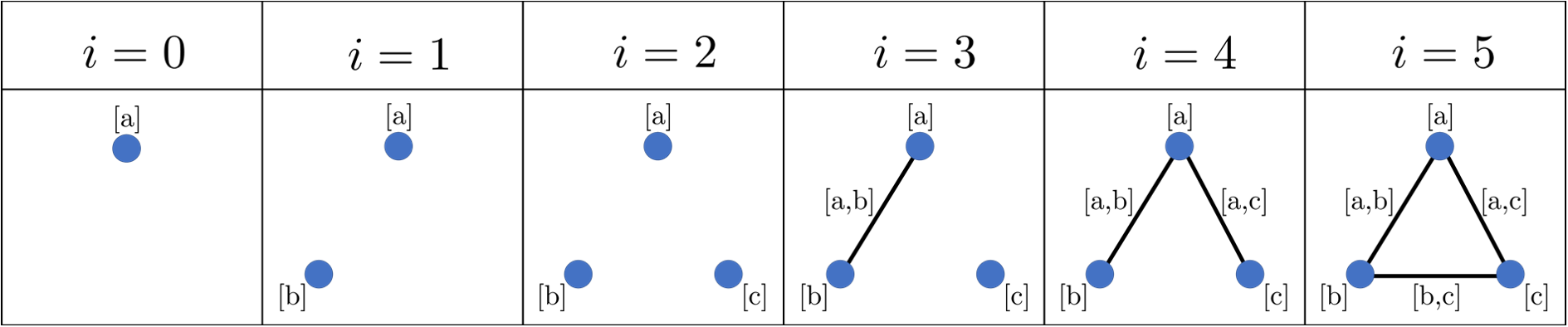
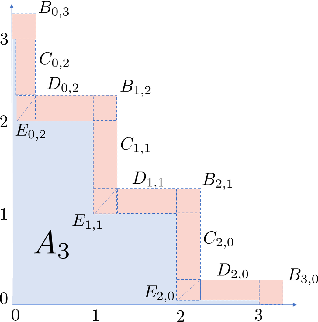
Let us see an example illustrating Theorem 1.1 and contrasting the categorical and tensor product filtrations. Indeed, consider the filtered simplicial complexes and shown in Figure 1.
The two filtrations and are shown in Figure 2. The products are computed in the category of ordered simplicial complexes using the order (see 3.9 and 3.10 for definitions).
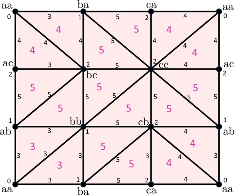
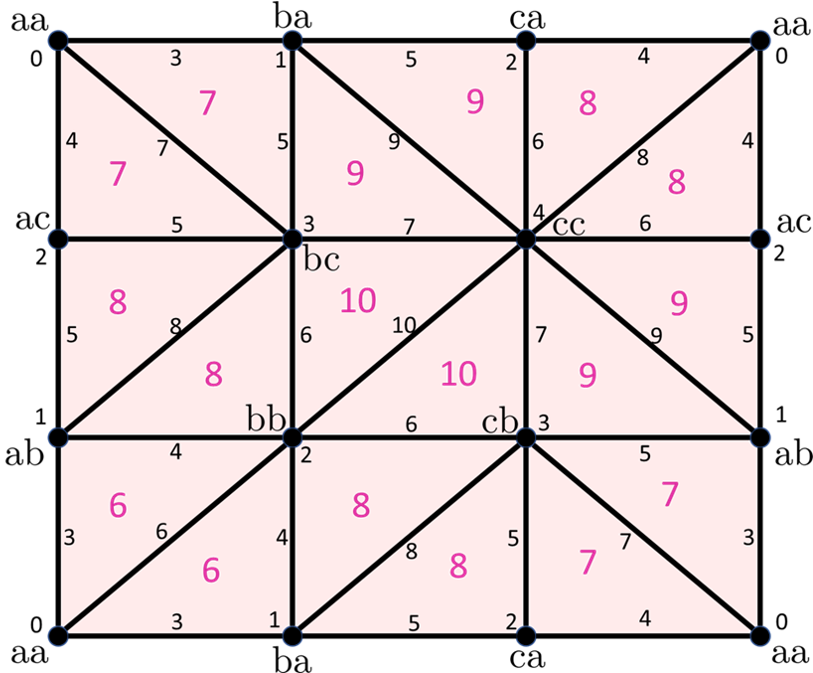
When comparing and , the first thing to note is the heterogeneity of indices in . This suggests that the tensor product filtration has more short-lived birth-death events than the categorical product, which is supported by the formulas in Theorem 1.1. That is, the barcodes of are expected to be “noisier” (i.e., with more short intervals) than those of . The barcodes for and from Figure 2, over any field , are shown in Figure 3.
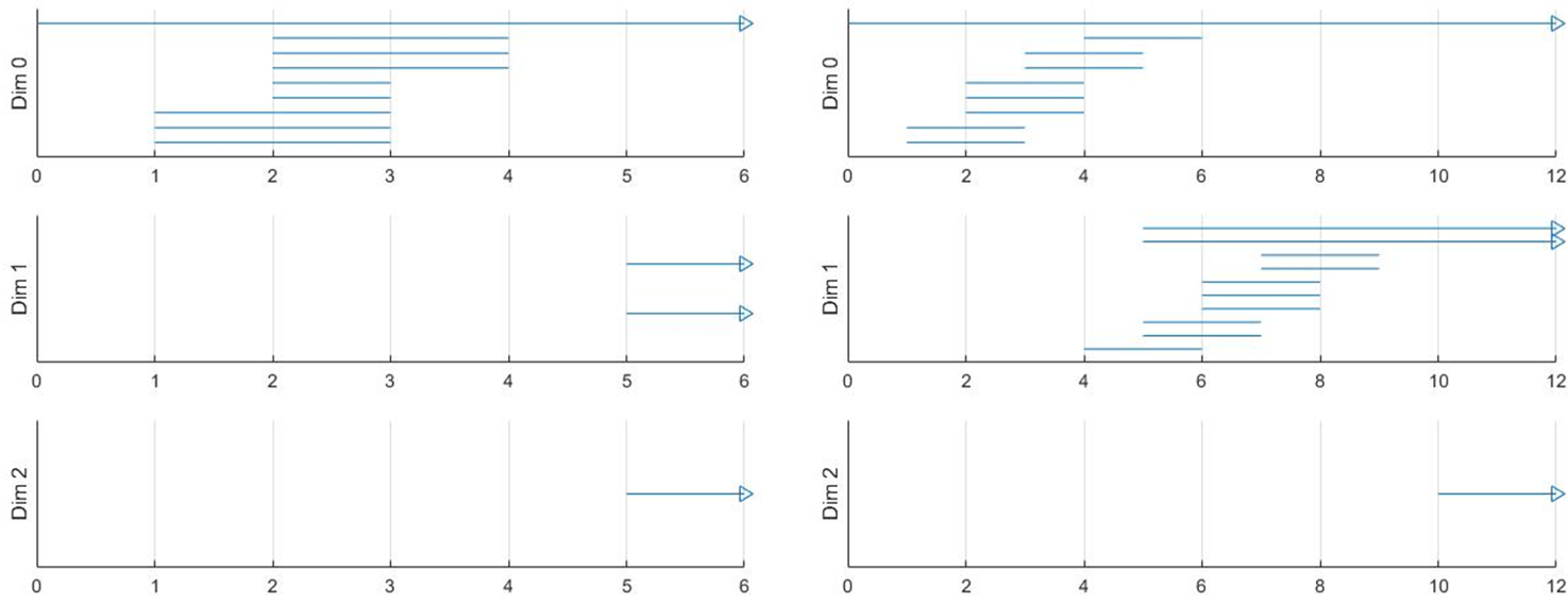
As described in Theorem 1.1, these barcodes are related to those of the complexes and , , where the subscripts denote homological dimension, as shown in Tables 2 and 2.
1.1. Sketch of proof
In establishing the formulae, the categorical product is the simpler of the two. Given two diagrams of topological spaces and continuous maps
indexed by a separable toally ordered set — e.g., the reals — so that is the identity of and for (similarly for ), we let . The classical topological Künneth theorem implies that the induced -indexed diagram
is isomorphic to
and a barcode computation, in the pointwise finite case, yields the result.
The tensor product of and requires a bit more work. Define the persistent homology of as
This object has the structure of a graded module over the polynomial ring in one variable , where the product of with a homogeneous element of degree reduces to applying the linear transformation induced by the inclusion . For purely algebraic reasons—specifically the algebraic Künneth theorem for chain complexes of flat modules over a PID—and a new persistent version of the Eilenberg-Zilber theorem (Theorem 5.10), one obtains a natural short exact sequence
| (6) | ||||
which splits, though not naturally. This is why we think of as the algebraic answer to asking what an appropriate notion of product filtration is: unlike , the tensor product fits into the type of short exact sequence one would expect in a Künneth theorem for persistent homology. The barcode formula in Theorem 1.1 follows, in the pointwise finite case, from the existence of graded -isomorphisms
with the convention that , using that (6) splits, and computing the tensor and Tor -modules explicitly in terms of operations on intervals.
We further establish that (6) still holds when the inclusions and are replaced by continuous maps and , respectively. In this case is replaced by a generalized tensor product , equivalent to for inclusions, and defined as follows: the space is the homotopy colimit of the functor from the poset to sending to , and to the map . The map is the one induced at the level of homotopy colimits by the inclusion of indexing posets.
1.2. Organization of the paper
Section 2 is devoted to the algebraic background needed for the paper; it takes a categorical viewpoint and introduces notions such as persistent homology, the classical Künneth theorems, and homotopy colimits. In section 3 we define products of (diagrams of) spaces and study their properties, while sections 4 and 5 contain the proofs of our persistent Künneth formulae for the categorical and generalized tensor products, respectively. In section 6 we present two applications of the Künneth formula for the categorical product in the setting of Vietoris-Rips complexes. The first application is to faster computations of the persistent homology of , and the second application revisits theoretical results about the Rips persistent homology of the -torus.
1.3. Related work
Different versions of the algebraic Künneth theorem in persistence have appeared in the last two years. In [42, Proposition 2.9], the authors prove a Künneth formula for the tensor product of filtered chain complexes, while [12, Section 10] establishes Künneth theorems for the graded tensor product and the sheaf tensor product of persistence modules. In [14], the authors prove a Künneth formula relating the persistent homology of metric spaces to the persistence of their cartesian product equipped with the (sum) metric , for homological dimensions . The persistent Künneth theorems proven here are the first to start at the level of filtered spaces, identifying the appropriate product filtrations and resulting barcode formulas. Compared to the sum metric [14], we remark that our results for the maximum metric hold in all homological dimensions.
2. Preliminaries
This section deals with the necessary algebraic background for later portions of the paper. We hope this will make the presentation more accessible to a broader audience, though experts should feel free to skip to Section 3 and come back as necessary. We provide a brief review of persistent homology, the rank invariant, the algebraic Künneth formula for the tensor product of chain complexes of modules over a Principal Ideal Domain (PID), as well as an explicit model for the homotopy colimit of a diagram of topological spaces. For a more detailed treatment we refer the interested reader to the references therein.
2.1. Persistent homology
The framework we use here is that of diagrams in a category (see also [13]). Besides the definitions and the classification via barcodes, the main point from this section is that the persistent homology of a diagram of spaces is isomorphic to the standard homology of the associated persistence chain complex (see [52] and Theorem 2.21).
Definition 2.1.
If and are categories, with small (i.e., so that its objects form a set), then we denote by the category whose objects are functors from to , and whose morphisms are natural transformations between said functors. The objects of the functor category are often referred to in the literature as -indexed diagrams in . Two diagrams are said to be isomorphic, denoted , if they are naturally isomorphic as functors.
Here is an example describing the main type of indexing category we will consider throughout the paper.
Example 2.2.
Let be a partially ordered set (i.e., a poset). Let denote the category whose objects are the elements of , and a unique morphism for each pair in . We call the poset category of .
As for the target category , we will mostly be interested in spaces and their algebraic invariants.
Example 2.3.
If Top is the category of topological spaces and continuous maps, and is a thin category (i.e., with at most one morphism between any two objects), then each object of is a collection of topological spaces , and continuous maps for each morphism in satisfying: is the identity of , and for any . Similarly, a morphism from to is a family of maps such that for every .
Example 2.4.
Let with its usual (total) order, and let be its poset category. -indexed diagrams in arise in Topological Data Analysis (TDA) as follows. Let be a metric space, let be a subspace and let be finite. In applications is the data one observes (e.g., images, text documents, molecular compounds, etc), obtained by sampling from/around (the ground truth, which is unknown in practice), both sitting in an ambient space . With the goal of estimating the topology of from , one starts by letting be the union of open balls in of radius centered at points of . Hence provides a—perhaps rough—approximation to the topology of for each , and any discretization of yields an object in as follows: , and the inclusion is the map associated to . Such objects allow one to avoid optimizing the choice of a single , leading to several recovery theorems and algorithms for topological inference [35].
Remark 2.5.
If each in is an inclusion, e.g. as in Example 2.4, then defines a filtered topological space. Specifically, the union of the ’s. Recall that a filtered topological space consists of a space together with a filtration .
This observation motivates the following definition.
Definition 2.6.
We call a filtered space if all its maps are inclusions. The collection of all filtered spaces forms a full subcategory of denoted FTop.
Example 2.7.
Let , and let be the functor defined as follows. For , let be the mapping telescope of
Explicitly, is the quotient space
It readily follows that whenever , and therefore defines an object in called the telescope filtration of .
As is typical in algebraic topology, one is interested in the interplay between diagrams of spaces and diagrams of algebraic objects.
Example 2.8.
Let be a commutative ring with unity, and let be the category of (left) -modules and -morphisms. The typical objects in one encounters in TDA arise from objects by fixing and taking singular homology in dimension with coefficients in . Indeed, is an -module for each , and for each morphism in , the map induces—in a functorial manner—a well-defined -morphism from to . The resulting object in will be denoted .
Definition 2.9.
Let , and let be the functor sending to , and each morphism in to
We say that is indecomposable if only when either or is the zero functor. Similarly, let be the functor sending to and to , where the tensor product is the usual one for -modules and -morphisms.
Example 2.10.
Recall that an interval in a poset is a set for which and always imply . An interval defines an object in as follows: for in , let
The ’s are called interval diagrams, and if is totally ordered, then they are indecomposable in [13, Lemma 4.2]. Moreover, if are intervals, then the tensor product of the corresponding interval diagrams satisfies
Indeed, if , and if , where the last isomorphism is given by multiplication in . Since applying and then multiplying equals multiplying and then applying , the result follows.
Interval diagrams are fundamental building blocks in [21, Theorem 1.1]:
Theorem 2.11.
Let be a field and let be a totally ordered set. Suppose that is separable with respect to the order topology, and that satisfies for all . Then, there exists a multiset of intervals called the barcode of , denoted , and so that
Moreover, only depends on—and uniquely determines—the isomorphism type of .
Remark 2.12.
An object satisfying the condition for all is said to be pointwise finite.
Definition 2.13.
Let and be as in Theorem 2.11, and let be so that is pointwise finite. The barcode of , denoted , is the unique multiset of intervals in such that
It follows that provides a succinct description of the isomorphism type of . The design of algorithms for the computation of barcodes, at least in the -indexed case, leverages a more concrete description of which we describe next.
Definition 2.14.
For an object in , let
| (7) |
is called the persistence module associated to .
The word module stems from the following observation: if , then is a graded module over , the graded ring of polynomials in a variable . Indeed, the -module structure is defined through multiplication by as follows: for let
and extend the action to in the usual way. The graded nature of the multiplication comes from noticing that for every .
If is a morphism in , then it can be readily checked that is a graded -morphism, and that defines a functor satisfying:
Theorem 2.15 (Correspondence).
Let denote the category of graded -modules and graded -morphisms. Then, is an equivalence of categories.
Remark 2.16.
Let in , and let be the resulting interval diagram. Then,
as graded -modules, with the convention . These are called interval modules.
Let —for instance, encoding multiscale approximations to the topology of an underlying unknown space (see Example 2.4). Applying as in Example 2.8 yields an object in , and applying the functor from the Correspondence Theorem (2.15) defines a graded -module. Explicitly:
Definition 2.17.
Given an object , its -dimensional persistent homology with coefficients in is the persistence module ,
Remark 2.18.
If is a field and is pointwise finite, then
as graded -modules. A graded version of the structure theorem for modules over a PID implies that if is finitely generated over , then can be recovered from the (graded) invariant factor decomposition of . This is how the first general persistent homology algorithms were implemented [52].
Thus far we have described persistent homology in terms of barcodes and -graded modules. The next, and final description, is in terms of the standard homology of the persistence chain complex. Indeed, let denote the category of (-graded) chain complexes of -modules, and chain maps. Recall that given two chain complexes and , their direct sum is given by
Definition 2.19.
Let be an object in . That is, each is a chain complex of -modules, and the ’s are chain maps. Then, the persistence chain complex of is
where each , and therefore is an object in the category of chain complexes of graded -modules.
Remark 2.20.
Since homology commutes with direct sums of chain complexes, then
as modules.
For , let denote the chain complex of singular chains in with coefficients in . Then, given , composition of functors yields an object in . The associated persistence chain complex is thus an object in and its homology—by Remark 2.20—recovers the persistent homology of . In other words,
Theorem 2.21 ([52]).
Let . Then, its persistent homology is isomorphic over to the homology of :
| (8) |
For a general (small) indexing category the barcode is no longer available as a discrete invariant for pointwise finite objects in [17]. However, it is always possible to consider the rank invariant:
Definition 2.22.
Let . The rank invariant of is the function on morphisms of given by . For an object we let .
2.2. The Classical Künneth Theorems
The classical Künneth theorem in algebraic topology relates the homology of the product of two spaces to the homology of its factors. The relation is via a split natural short exact sequence, and the proof is a combination of the algebraic Künneth formula for chain complexes, and the Eilenberg-Zilber theorem. Both theorems are stated next, but first here are two relevant definitions:
Definition 2.24.
Let be a commutative ring, and let . The tensor product chain complex consists of -modules and boundary morphisms
Definition 2.25.
An -module is called flat, if for every short exact sequence of -modules, the induced sequence
is also exact. In particular, free modules are flat.
Theorem 2.26 (The Algebraic Künneth Formula).
If is a PID and at least one of the chain complexes is flat (i.e., the constituent modules are flat), then for each there is a natural short exact sequence
which splits but not naturally.
See for instance [32, Chapter 5, Theorem 2.1]. As it is well known, when and are the singular chain complexes of two topological spaces and , then the Eilenberg-Zilber theorem [28] provides a link between the algebraic Künneth theorem and the homology of :
Theorem 2.27 (Eilenberg-Zilber).
For topological spaces and , there is a natural chain equivalence , and thus
for all .
The existence of is in fact an application of the acyclic models theorem of Eilenberg and MacLane [26]. This theorem provides conditions under which two functors to the category of chain complexes produce naturally isomorphic homology theories. Later on we will use the machinery of acyclic models to prove a persistent Eilenberg-Zilber theorem (Theorem 5.10), which then yields our persistent Künneth formula for the tensor product (Theorem 5.12). For now, here is the topological Künneth theorem:
Corollary 2.28 (The topological Künneth formula).
Let be topological spaces and let be a PID. Then, there exists a natural short exact sequence
| (9) | ||||
which splits, though not naturally.
2.3. Homotopy Colimits
The machinery of homotopy colimits will be used in Section 3 to define the generalized tensor product appearing in Theorem 5.12. We provide here a basic review, but direct the interested reader to [25] or [49] for a more comprehensive presentation. If is a category, then will denote its opposite category, and will denote its classifying space—i.e., the geometric realization of the nerve of .
Definition 2.29.
The undercategory of , denoted , is the category whose objects are pairs consisting of an object and a morphism in . A morphism from to is a morphism in such that .
Remark 2.30.
If is a morphism in , then composing with induces covariant functors and .
Definition 2.31.
Let be a family of objects in a category . The product of this family, if it exists, is an object along with morphisms such that for any and any collection of morphisms , there exists a unique morphism so that for each . The product, since when it exists it is unique up to isomorphism, will be denoted . The existence of for any and any , is referred to as the universal property defining the categorical product.
The dual notion of coproduct of is the object , when it exists, along with morphisms such that for any any object and any collection of morphisms , there exists a unique morphism such that for each . The coproduct of is denoted , and the existence of is the universal property defining it.
Example 2.32.
If , then the product is the space whose underlying set is the Cartesian product endowed with the product topology, while the coproduct is their disjoint union.
Definition 2.33.
Let be morphisms in a category . The coequalizer of and , denoted if it exists, is an object with a morphism such that . Moreover, if there is another pair such that , then there is a unique such that .
Example 2.34.
If are two morphisms in , then is the quotient space .
Definition 2.35.
Let be a functor. The colimit of is defined as:
| (10) |
where the top map sends to itself via the identity, the bottom map sends to via , and the first coproduct is indexed over all morphisms in . Similarly, the homotopy colimit of is defined as:
| (11) |
The top map is times the identity, while the bottom map is the identity of times the map on classifying spaces induced by .
It is worth noting that if , then any morphism induces (functorially) a map , and that if and , then induces a natural map called the change of indexing category. Moreover, [25]
Proposition 2.36.
Let , and be functors. Then .
While both the colimit and the homotopy colimit of a diagram of spaces yield methods for functorially gluing spaces along maps, only the latter preservers homotopy equivalences. Indeed [49, Proposition 3.7],
Theorem 2.37.
Let . If is a natural (weak) homotopy equivalence—i.e. each is a (weak) homotopy equivalence—then the induced map is a (weak) homotopy equivalence.
When the indexing category has a terminal object, that is, a unique object such that for all there is a unique morphism , then the homotopy colimit is particulary simple [25, Lemma 6.8],
Theorem 2.38.
Suppose that has a terminal object . Then for all , the collapse map is a weak homotopy equivalence.
Notice that by collapsing the classifying spaces and in the definition of homotopy colimit to a point, we recover the definition of the colimit. Next, we will see specific conditions under which this collapse defines a homotopy equivalence from to . In order to state the result, we recall the notion of a cofibration.
Definition 2.39.
A continuous map is called a cofibration if it satisfies the homotopy extension property with respect to all spaces . That is, given a homotopy and a map such that , then there is a homotopy such that for all . If is a closed subset of , then is called a closed cofibration.
Remark 2.40.
The telescope filtration of satisfies that is a closed cofibration for all [10, Chapter VII, Theorem 1.5].
Here is one situation where and provide similar answers,
Lemma 2.41 (Projection Lemma).
Let be a partially ordered set and its poset category. Let be such that is a closed cofibration for each pair in . Then the collapse map
is a homotopy equivalence.
Proof.
See [49, Proposition 3.1]. ∎
3. Products of Diagrams of Spaces
With the necessary background in place, we now move towards the main results of the paper. Given a category of spaces (e.g., topological, metric, simplicial, etc) and a small indexing category , our first objective is to identify relevant products between -indexed diagrams . For a particular product, the goal is to describe its persistent homology in terms of the persistent homologies of and . This is what we call a persistent Künneth formula. Let us begin with the first product construction: the categorical product in .
Definition 3.1.
Let be a category having all pairwise products (e.g., finitely complete), let , and let be the functor taking each object to the (categorical) product , and each morphism in to the unique morphism making the following diagram commute:
| (12) |
The existence of follows from the universal property defining .
We have the following observation:
Proposition 3.2.
Let be a category with all pairwise products. Then, is the categorical product of .
Proof.
First, note that the existence of and follows from that of and for each , and the commutativity of (12) for each .
Let , and let , be morphisms. For each , let be the unique morphism so that and . It readily follows that , given by , is the unique morphism of -indexed diagrams such that , and . ∎
Let us describe in more detail the categories we have in mind for , as well as what the categorical products are in each case.
Example 3.3 (Topological spaces).
Recall that denotes the category of topological spaces and continuous maps. For , their Cartesian product equipped with the product topology is the categorical product of and in .
Example 3.4 (Metric Spaces).
Let denote the category of metric spaces and non-expansive maps. That is, its objects are pairs —a set and a metric— and its morphisms are functions so that for all .
Definition 3.5.
Given , let denote the Cartesian product of the underlying sets, and let be the maximum metric on :
Since the coordinate projections and are non-expansive, it readily follows that is the categorical product of and in .
Example 3.6 (Simplicial Complexes).
Recall that a simplicial complex is a collection of finite nonempty sets—called simplices—so that if and , then . Let be the collection of simplices of with elements—these are called -simplices and we write instead of . A function between simplicial complexes is called a simplicial map if for every . Let be the category of simplicial complexes and simplicial maps.
Definition 3.7.
For , let be the smallest simplicial complex containing all Cartesian products , for and .
In other words, if and only if there exist and with . Let and be the projection maps onto the first and second coordinate, respectively. Since , then , and similarly . Hence and define simplicial maps , and it readily follows that is the categorical product of and in .
As mentioned in the Introduction, the Rips complex at scale is a simplicial complex which can be associated to any metric space . It is widely used in TDA—when is the observed data set—and it is defined as
| (13) |
Notice that any non-expansive function between metric spaces extends to a simplicial map , and thus defines a functor from to . This functor is in fact compatible with the categorical products:
Lemma 3.8.
Let , be metric spaces, and let . Then,
Proof.
See the proof of Proposition 10.2 in [1]. ∎
One drawback of the categorical product in is that it is not well-behaved with respect to geometric realizations. Indeed, recall that the geometric realization of a simplicial complex —denoted —is the collection of all functions so that , and for which . Moreover, if , then
defines a metric on . Every simplicial map induces a function given by
which, as one can check, is non-expansive. In other words, geometric realization defines a functor . To see the incompatibility of and the product in , let . It follows that is (homeomorphic to) the geometric 3-simplex , while is the unit square . Hence, is in general not equal, nor homeomorphic to . This leads one to consider other alternatives; specifically, the category of ordered simplicial complexes.
Example 3.9 (Ordered Simplicial Complexes).
If comes equipped with a partial order so that each simplex is totally ordered, then we say that is an ordered simplicial complex. A simplicial map between ordered simplicial complexes is said to be order-preserving, if it is so between 0-simplices. Let denote the resulting category. For data analysis applications, and particularly for the Rips complex construction, is perhaps more relevant than . Indeed, a data set stored in a computer comes with an explicit total order on . If , with partial orders , respectively, and , , then the Cartesian product has a partial order given by if and only if and .
Definition 3.10.
For , let be defined as follows: if and only if there exist and so that is a totally ordered subset of , with respect to .
Just like for simplicial complexes, the coordinate projections and induce order-preserving simplicial maps and . Moreover,
Lemma 3.11.
Let and be ordered simplicial complexes. Then,
-
(1)
is their categorical product in .
-
(2)
, where the right hand side is the categorical product in . Moreover, is a deformation retract of .
-
(3)
The product map is a homeomorphism.
Proof.
See [27], specifically Definitions 8.1, 8.8 and Lemmas 8.9, 8.11. ∎
The above are the categories of spaces and the products we will consider moving forward. Going back to diagrams in , recall that a CW-complex is a topological space together with a CW-structure. That is, a filtration of , so that has the discrete topology, is obtained from by attaching -dimensional cells via continuous maps , and so that the topology on coincides with the weak topology induced by . It follows that . In this context, a cellular map between CW-complexes—i.e. a continuous function so that for all —is exactly a morphism in . Thus, if denotes the category of locally compact CW-complexes (we will see in a moment why this restriction) and cellular maps, then is a full subcategory of .
If and are CW-complexes, then their topological product can also be written as a union of cells. Specifically, the -cells of are the products with , for an -cell of , and a -cell of . Thus, if
| (14) |
then will be a CW-structure for provided the product topology coincides with the weak topology induced by (14). If either or are locally compact, then this will be the case (see Theorem A.6 in [31]).
In summary: the categorical product in does not recover the usual product of CW-complexes, which suggests the existence of other useful (non-categorial) products in and . The product of CW-complexes suggests the following definition,
Definition 3.12.
If , then their tensor product is the filtered space
The tensor product of filtered spaces is sometimes regarded in the literature as the de facto product filtration; see for instance [8, 11, 43] or [44, Chapter 27]. For general objects in —e.g., when the internal maps are not inclusions—taking the union of, say, and does not make sense. Instead, the corresponding operation would be to glue these spaces along the images of the product maps
Here is where the machinery of homotopy colimits comes in as a means to defining a generalized tensor product in :
Definition 3.13.
For , let be the poset category of with its usual product order, and for , let
be the functor sending to , and to . The generalized tensor product of and is the object given by
| (15) | ||||
where the latter is the continuous map associated to the change of indexing categories induced by the inclusion .
Remark 3.14.
The definition of the generalized tensor product can be extended to diagrams indexed by other subcategories of . For example, to the poset categories of , (the set of non negative reals) and (the set of positive reals). In general, for , , , or , we let and define as in (15). Although and are different for each choice of , we will use the same notation for aesthetic purposes. The choice will be clear from the context as we will specify the in .
We have the following relation between and ,
Lemma 3.15.
Let , and let be their telescope filtrations. Then, is naturally homotopy equivalent to .
Proof.
We will show that there is a morphism , so that each map , , is a homotopy equivalence. Indeed, since deformation retracts onto , then each inclusion is a homotopy equivalence, and thus (by Theorem 2.37) so is the induced map
Since each inclusion is a closed cofibration (Remark 2.40), then the projection Lemma 2.41 implies that the collapse map
is a homotopy equivalence. Moreover, since all the maps in are inclusions, and the colimit of such a diagram is essentially the union of the spaces, then there is a natural homeomorphism
which completes the proof. ∎
It follows that,
Corollary 3.16.
If , then as graded -modules.
Later on—when studying the persistent singular chains of —it will be useful to have Proposition 3.17 below. The setup is as follows: observe that if and , then
is an open neighborhood of in , which deformation retracts onto . Indeed, any element can be written uniquely as where either and , or for and . In these coordinates , and a deformation retraction can be defined as
| (16) |
Let be and . Then,
Proposition 3.17.
If and , then formation retracts onto , and deformation retracts onto .
Proof.
Given , our goal is to define a deformation retraction
To this end, we subdivide as follows: For , let
We further write where (sim. ) if and only if (sim. ). Figure 4 below visually represents the subsets defined above for .
Let us now define the map . Let be the projection onto the first coordinate. On each we define
where are given by (16). For elements in , takes to
And finally, for elements in , takes to
Continuity readily follows by construction. Furthermore, the marginal function is the identity everywhere and . This finishes the proof. ∎
3.1. A comparison theorem
Next we show that the persistent homology of the categorical and generalized tensor products are interleaved in the log scale. While a full characterization of stability for each product filtration is beyond the scope of this paper, this section showcases some of the techniques one can employ when addressing this question.
Definition 3.18.
For , the -shift functor is defined as follows: For , let be the functor sending to , and to . For a morphism , we get a morphism , and if , then there is a morphism satisfying
for all . We call the -transition morphism.
The notion of interleavings, first introduced in [18], allows one to compare objects in . Specifically:
Definition 3.19.
Let and . A -interleaving between and consists of morphisms and so that and . We define the interleaving distance between and as:
If there are no interleavings between and , we say that .
Let denote the poset category associated to the set of positive reals, , and define the logarithm functor as
Then,
Theorem 3.20.
If , then
Proof.
For each , let . We have inclusions and , and thus by Proposition 2.36, the triangles in the diagram
| (17) |
commute. Since has a terminal object, namely , then the natural map
is a weak homotopy equivalence (Theorem 2.38). Such maps induce isomorphisms at the level of homology [31, Theorem 4.21], and thus applying followed by turns (17) into a -interleaving of the desired objects in . ∎
If are pointwise finite, then—in addition to their interleaving distance —one can compute the bottleneck distance between and as follows. A matching between two multisets and is a multiset bijection between some and . Given , we say that and are matched, and all other elements of are called unmatched. Let . A matching between and is called a -matching if the following conditions hold:
-
(1)
If and are matched, then
Recall that and are, respectively, the left and right endpoints of the interval .
-
(2)
If is unmatched, then .
The bottleneck distance between and is defined as:
If no -matchings exist, then the bottleneck distance is .
The Isometry Theorem [7] implies that if are pointwise finite, then
The following corollary is a direct consequence of the above equality and Theorem 3.20.
Corollary 3.21.
Let be so that and are pointwise finite. Then
-
(1)
If under a matching realizing —which exists by [19, Theorem 5.12]—we have that is matched to , then
-
(2)
If is unmatched, then
4. A Persistent Künneth formula for the categorical product
Let be a small indexing category and let be any of the categories of spaces from Section 3 (that is = , , , or ). In this section we relate the rank invariants of two objects in to that of their categorical product, and prove the persistent Künneth formula for the categorical product in , where is the poset category of a separable totally ordered poset .
Remark 4.1.
Recall that the topological Künneth formula (Corollary 2.28) holds for objects and singular homology. Every can be viewed as a topological space via the metric topology, and since the maximum metric induces the product topology, then the Künneth formula holds for . Let , and let be the geometric realization functor. From the homeomorphism and the natural isomorphism between singular and simplicial homology, the formula holds in . Using (2) of lemma 3.11, the formula also holds for .
Let be a field and let and be objects in . Using the topological Künneth formula and the observation that and are vector spaces for each , , we obtain isomorphisms
Using naturality, this yields an isomorphism in between and , where
| (18) |
and the homomorphism is the sum of the ones induced between tensor products by the maps and . In other words, and using the notation of tensor product and direct sum of objects in (see Definition 2.9), we obtain the following:
Lemma 4.2.
If , then for every and every field
in .
An immediate consequence is the following calculation at the level of rank invariants (see Definition 2.22):
Proposition 4.3.
Let and let , be their rank invariants. Then
for every in , with the convention that .
Proof.
This follows by direct inspection of the homomorphism
for each . Indeed, since , then the result follows from the fact that the dimension of the tensor product of two vector spaces equals the product of the dimensions. ∎
We are now ready to prove the main result of this section: the Künneth formula for the categorical product .
Theorem 4.4.
Let be the poset category of a separable (with respect to the order topology) totally ordered set. Let be -indexed diagrams of spaces, and assume that and are pointwise finite for each . Then is pointwise finite, and its barcode satisfies:
where the union on the right is of multisets (i.e., repetitions may occur).
Proof.
The fact that is pointwise finite follows directly from Lemma 4.2. As for the barcode formula, and removing the field from the notation, we have the following sequence of isomorphisms
The direct sum distributes with respect to the tensor product in since it does so in . The last isomorphism is the one from Example 2.10, and the theorem follows from the uniqueness of the barcode. ∎
This result generalizes to the product of objects in by inductively using and to compute :
Corollary 4.5.
Let . Assume that for each , , is pointwise finite. Then
The result which is perhaps most relevant to persistent homology computations with Rips complexes is as follows:
Corollary 4.6.
Let be finite metric spaces and let be the barcode of the Rips filtration . Then,
for all , if is the maximum metric.
5. A Persistent Künneth formula for the generalized tensor product
We will now establish the Künneth formula for the generalized tensor product of two objects . We start with a brief discussion on the grading of the tensor product and Tor of two graded modules over a graded ring . The discussion then specializes to in order to establish the -isomorphisms
| (19) | ||||
for . We end with a persistent Eilenberg-Zilber theorem, from which the aforementioned persistent Künneth theorem will follow.
5.1. The tensor product and Tor of graded modules
Recall that a commutative ring with unity is called graded if it can be written as where each is an additive subgroup of and for every . Similarly, an -module is graded if it can be written as , where the ’s are subgroups of and for all . An element (resp. in ) is called homogeneous of degree if (resp. in ), and we will use the shorthand .
Let be graded modules over a graded ring . Our first goal is to describe a direct sum decomposition of the -module inducing the structure of a graded -module. Indeed, since and are -modules for all , then so are and we have the -isomorphism
Fix and let be the -submodule of generated by elements of the form , where , and are homogeneous elements with . It follows that is a submodule of
and thus if . Let . Any homogeneous element of degree induces a well-defined -homomorphism
and therefore
| (20) |
inherits the structure of a graded -module.
The inclusion induces an -epimorphism with . Indeed, the elements of are exactly the relations missing between and when defining the latter as a quotient module. It follows that induces an isomorphism
of -modules, and the grading on the codomain induced by (20) turns into a graded isomorphism of graded -modules. We summarize this analysis as follows:
Proposition 5.1.
Let be graded modules over a graded ring . Then decomposes as the direct sum of the subgroups
and for all . In other words, is a graded -module.
And now we prove the proposition for :
Proposition 5.2.
If are graded -modules, then so is .
Proof.
Fix a graded free resolution
defined inductively as follows. Let be the free -module generated by the homogeneous elements of , and define for each the additive subgroup
Then , and with this decomposition, the natural map is a surjective graded homomorphism of graded -modules. In particular, the kernel of this homomorphism is a graded -submodule of . We proceed inductively by letting be the graded free -module generated by the homogeneous elements in the kernel of .
Taking the tensor product with over yields
and we note that:
-
(1)
Each is a graded -module, by Proposition 5.1, and each is a graded -homomorphism.
-
(2)
decomposes as the direct sum
and similarly, decomposes as
with the image being a graded -submodule of the kernel.
-
(3)
inherits the structure of a graded -module from the decomposition
finishing the proof. ∎
We now specialize to the case and present explicit computations for interval modules. For , let denote the graded -module . For brevity, we will drop the subscript if it is . That is, we will use to denote . Then, and .
Proposition 5.3.
Let , . Then and .
Proof.
There is a graded -isomorphism , which takes the generator to . Since and are quotient modules of and respectively, their tensor product is isomorphic to a quotient module of , say for some appropriate . The isomorphism takes to and the action of gives . The left hand side is zero if either is zero in or if is zero in . This implies that if , then is zero in . The minimum of all such is and therefore, .
To compute , we fix a graded free resolution for :
Taking the tensor product of the sequence with gives us:
Using the definition of and the tensor product of intervals, we get that
where the last isomorphism is justified by the following argument: the element goes to where . The latter is zero if and only if , or said equivalently . This finishes the proof. ∎
Remark 5.4.
This last proposition recovers the formulas shown in (19). Moreover, using bilinearity, these isomorphisms can be used to compute the tensor product and Tor of any pair of finitely generated graded -modules.
5.2. The Graded Algebraic Künneth Formula
The Algebraic Künneth Formula for graded modules over a graded PID is proved in exactly the same way as Theorem 2.26, by noticing that all the steps can be carried out in a degree-preserving fashion. A few versions of this have appeared recently, see for instance [42, Proposition 2.9] or [12, Theorem 10.1], and we include it next for completeness:
Theorem 5.5.
Let and be two chain complexes of graded modules over a graded PID , and assume that one of is flat. Then, for each , there is a natural short exact sequence
which splits, though not naturally.
It is at this point that we depart from the existing literature on persistent Künneth formulas for the tensor product of filtered chain complexes. Indeed, next we will turn these algebraic results into theorems at the level of filtered topological spaces. We begin with the following result:
Theorem 5.6.
Let . Then, for all , we have a natural short exact sequence
which splits, but not naturally.
Proof.
Since and are filtered spaces, then and are chain complexes of free graded -modules, and hence flat. Now, each inclusion is a homotopy equivalence, and thus induces an isomorphism at the level of homology. One thing to note is that if , then
commutes only up to homotopy, but this is enough to conclude that induces natural isomorphisms , . The result follows from plugging and into Theorem 5.5, and using the natural -isomorphisms . ∎
5.3. A Persistent Eilenberg-Zilber theorem
Our next objective is to show that the chain complexes and have naturally isomorphic homology. The result follows, as we will show in Theorem 5.11, from applying the machinery of acyclic models [26] to the functors
Here is the full subcategory of comprised of those filtered spaces where is an open subset of for all , and is the graded -module whose degree- component is the sum of vector spaces
where each is regarded as a linear subspace of . The models in question are a family of objects from satisfying certain properties (Lemmas 5.7 and 5.8) implying our Persistent Eilenberg-Zilber Theorem 5.10. We start by defining .
For , let be the filtered space with the empty set at indices , and for :
Let be the standard geometric -simplex, and let be the set of objects in for . We have the following:
Lemma 5.7.
Each is both -acyclic and -acyclic. That is, the homology groups and are trivial for all .
Proof.
If , then
as chain complexes of graded -modules. Since is convex, then
for all , showing that is -acyclic.
To show that is -acyclic, notice that for , and that is a free graded -module. By the graded algebraic Künneth Theorem 5.5, with and , we get that
for all , since the tensor products and Tor modules in the short exact sequence are all zero. ∎
Lemma 5.8.
For each , the functors and are free with base in .
Proof.
Let . The functor (resp. ) being free with base in means that for all , the graded -module (resp. ) is freely generated over by some subset of
where ranges over all morphisms in from to .
Starting with , we will first construct a free -basis for
consisting of singular -simplices on the spaces . We proceed inductively as follows: Let be the collection of all singular -simplices , and assume that for a fixed and every we have constructed a set of simplices , , so that
is a basis, over , for
Since is an -submodule of and the latter is torsion free, then is an -linearly independent subset of . We claim that can be completed to an -basis of , consisting of singular -simplices , . Indeed, if is the collection of all sets of simplices , , so that is -linearly independent in and , then can be ordered by inclusion, and any chain in is bounded above by its union. By Zorn’s lemma has a maximal element , which yields the desired basis. If we let , then
is a free -basis for .
We claim that each is in the image of for some model and some morphism in . Indeed, since is of the form for some , then there are unique singular simplices and , so that if is the diagonal map , then . Let be the morphism in defined as the inclusion for , and as the composition for . Define in a similar fashion. Then, is a morphism in , and if
is the singular -simplex corresponding to the diagonal map , then
As for the freeness of
we note that each direct summand is freely generated over by elements which can be written as the tensor product of a homogeneous element from and a homogeneous element from . That is, by elements of the form , where and are singular simplices. We let and be defined as in the analysis of above. Let be the homogeneous element of degree corresponding to the identity of , and define in a similar fashion. Then, and
thus completing the proof. ∎
Lemma 5.9.
The functors and are naturally equivalent.
Proof.
Given , our goal is to define a natural isomorphism
The first thing to note is that the graded algebraic Künneth formula (Theorem 5.5) yields a natural isomorphism
Moreover, since each is open in , then the inclusion
is a chain homotopy equivalence (see [31, Proposition 2.21]), and thus
Therefore, it is enough to construct a natural isomorphism
and we will do so on each degree as follows. Recall that (see Proposition 5.1)
where is the linear subspace of generated by elements of the form with . Let
where (resp. ) is a path-connected component of (resp. ), , and is the unique path-connected component of containing . This definition on basis elements uniquely determines as an -linear map, and we claim that it is surjective with . Surjectivity follows from observing that if , then for some , and that if and are the path-connected components in and , respectively, so that , then path-connectedness of and maximality of imply .
The inclusion is immediate, since it holds true
for elements of the form
,
and these generate over .
In order to show that , we will
first establish the following:
Claim 1: If and are path-connected components, , such that , then
Indeed, let be a path with and . Since each is open in , then the Lebesgue’s number lemma yields a partition such that and for all . Let , and let be its path-connected component in . Since and , then it is enough to show that
Fix , assume that , and let (the argument is similar if ). Since the projection is a path in from to , then in . Similarly, the projection is a path in from to , and since , then in . This calculation shows that
and therefore . (end of Claim 1)
Let us now show that . To this end, let and write
where , and where the indices have been ordered such that there are integers , and distinct path-connected components of so that if , then for all . Since the ’s are linearly independent in , then implies
and therefore
where each summand is an element of , by Claim 1 above. Thus, , induces a natural -isomorphism
and letting completes the proof. ∎
We now move onto the main results of this section.
Lemma 5.10 (Persistent Eilenberg-Zilber).
For objects and coefficients in a field , there is a natural graded chain equivalence
with (Lemma 5.9), and unique up to a graded chain homotopy.
Proof.
The proof follows exactly that of Theorem 2.27 [28], using acyclic models [26] (see also the proof of Theorem 5.3 in [47] for a more direct comparison). Indeed, the functors in question are acyclic (Lemma 5.7), free (Lemma 5.8), and naturally equivalent at the level of zero-th homology (Lemma 5.9). ∎
Theorem 5.11.
If , then there is a natural -isomorphism
Proof.
Lemma 3.15 implies that , and Proposition 3.17 shows that if , then
Moreover, since , then the inclusion
is a graded chain homotopy equivalence (see [31, Proposition 2.21]), and thus Lemma 5.10 shows that
The can be removed since deformation retracts onto (Proposition 3.17), which completes the proof. ∎
Finally, we obtain
Theorem 5.12.
There is a natural short exact sequence of graded -modules
which splits, though not naturally.
Remark 5.13.
If is either , , , or , then following Remark 4.1 yields a similar Persistent Künneth theorem in each case.
5.4. Barcode Formulae
We now give the barcode formula for the generalized tensor product of objects in . Recall from Theorem 2.11 that pointwise finite objects in can be uniquely decomposed into interval diagrams. In Proposition 5.3, the tensor product and of the associated interval modules was computed, and the following is a consequence of Theorem 5.12.
Theorem 5.14.
Let . Assume that for , the diagrams and are pointwise finite. Then is pointwise finite with barcode
In the above formula, the first union of intervals is associated with the tensor part of the sequence in theorem 5.12, while the second union is associated with the part. The results are easy to generalize to -th persistent homology in the case of finite tensor product of objects in Top.
Corollary 5.15 (-th persistent homology).
Let , and assume that is pointwise finite for all . Let be the -dimensional barcode of , then
In other words, a bar in corresponding to bars, one from each , starts at the sum of the starting points and lives as long as the shortest one.
Topological inference deals with estimating the homology of a metric space from a finite point cloud , as discussed in Example 2.4. Usually, longer bars in a barcode represent significant topological features. The following corollary allows us to count the number of bars longer than a threshold in the barcode of the tensor product.
Corollary 5.16 (On high persistence).
For and , let and denote the number of bars with length exactly and at least respectively in . Assume that the lengths of longest bars in and are and respectively, then
and
| (21) |
By replacing with , the formula in equation 21 can be used to compute the number of bars with the longest length in .
6. Applications and Discussion
6.1. Application: Time series analysis
Time series are ubiquitous in data science and make for an important object of study. Recently, the problem of detecting recurrence in time varying-data has received increasing attention in the applied topology literature [38, 51]. Two types of recurrence that appear prominently are periodicity and quasiperiodicity. A function is said to be quasiperiodic on the -linearly independent frequencies if there exists so that each is periodic with frequency , and for all . Quasiperiodicity appears naturally in biphonation phenomena in mammals [50], and in transitions to chaos in rotating fluids [30].
The topological approach to recurrence detection starts with the sliding window embedding of , defined for each and parameters and , as
One then uses the barcodes for , as signatures; for if is periodic, then is a closed curve [40], and when is quasiperiodic then is dense in a high-dimensional torus [36, 29]. These ideas have been used successfully to find new periodic genes in biological systems [39], and to automatically detect biphonation in high-speed videos of vibrating vocal folds [45].
One of the main challenges in computing for a quasiperiodic time series is that if fills out the torus at a slow rate — requiring a potentially large — then the persistent homology computation becomes prohibitively large. We will see next how the categorical persistent Künneth formula (Corollary 4.6) can be used to address this. The general strategy will be illustrated with a computational example.
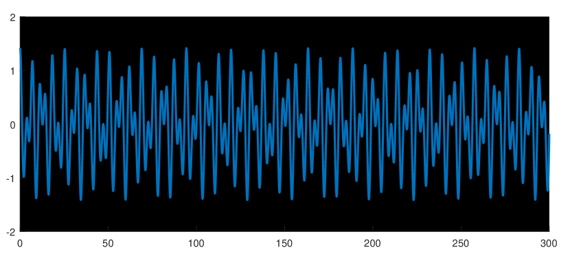
Let with , and let . If
then , where
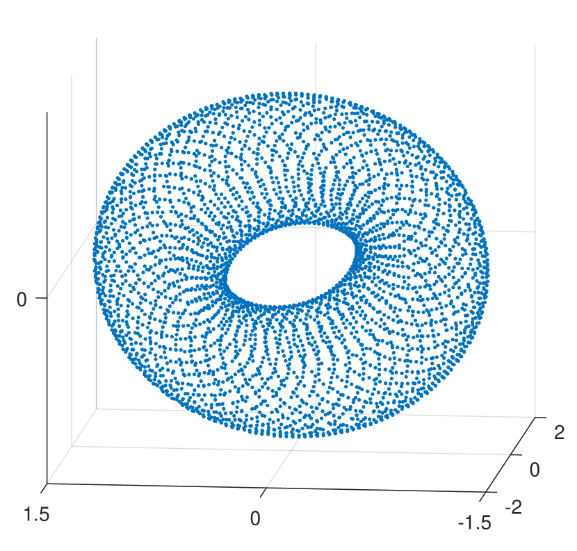
An elementary calculation shows that if and , then the columns of are orthonormal in . Fix , , as above, and . Figure 5 below shows the real part of (left), and a visualization (right) of the sliding window point cloud , , using Principal Component Analysis (PCA) [33].
Computing the exact barcodes , ,
for point clouds of this size is already prohibitively large (e.g., with Ripser [4]).
Thus, one strategy is to choose a smaller set of landmarks
and use the stability theorem [19]
to estimate the barcodes of using those of , up to an error (in the bottleneck sense) of twice the Gromov-Hausdorff distance between and . Specifically, if and satisfies , then there is a unique with , and thus
| (22) | ||||
In what follows we compare this landmark approximation procedure to a different strategy leveraging the categorical persistent Künneth theorem for the Rips filtration on the maximum metric (Corollary 4.6). Here is the setup:
- Landmarks:
-
We select a set of 400 landmarks ( of the data) using
maxminsampling. That is, is chosen at random and the rest of the landmarks are selected inductively asWe endow with the Euclidean distance in , and compute the barcodes , , directly using
Ripser[4]. - Künneth:
-
Let be the projections onto the first and second coordinate, respectively. We select two sets of landmarks, and with 70 points each using
maxminsampling, and endow the cartesian product with the maximum metric in . The barcodes of and are computed usingRipser, and we deduce those of for using Corollary 4.6.
6.1.1. Computational Results
Table 3 shows the computational times in each approximation strategy — i.e., via the landmark set and the persistent Künneth theorem applied to — as well as the number of data points in each case.
| Landmarks | Künneth | |
|---|---|---|
| Time (sec) | 15.22 | 0.20 |
| # of points | 400 | 4,900 |
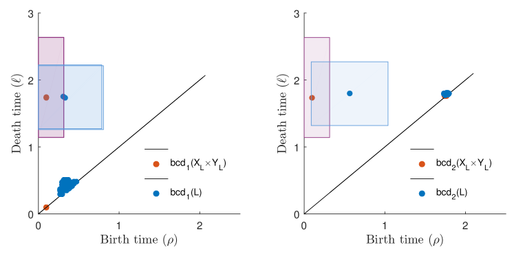
As these results show, the Künneth approximation strategy is almost two orders of magnitude faster that just taking landmarks, and as we will see below, it is also more accurate. Indeed, the inequalities in (22) can be used to generate a confidence region for the existence of an interval given a large enough interval . A similar region can be estimated from as follows. Since the columns of are orthonormal, then for every we have and thus
Moreover, (see 3.21) if satisfies
where is computed for subspaces of , then there exists a unique so that
| (23) | ||||
Figure 6 shows the resulting confidence regions for both approximation strategies. Each interval is replaced by a point , and the regions for (22) and (23) are shown in blue and red, respectively. We compare these regions by computing their area, and report the results in Table 4.
| Landmarks | Künneth | |
|---|---|---|
| 1 | 0.7677 | 0.4680 |
| 1 | 0.7480 | 0.4709 |
| 2 | 0.9072 | 0.4704 |
These results suggest that the Künneth strategy provides a tighter approximation than using landmarks. Moreover, both strategies can be used in tandem — improving the quality of approximation — via intersection of confidence regions.
6.2. Application: Vietoris-Rips complexes of -Tori
The main theorem in [1] implies that the Vietoris-Rips complex of a circle of radius (equipped with Euclidean metric) is homotopy equivalent to if
Consider the categorical product of Vietoris-Rips complexes on circles . We know it is homotopy equivalent to where equipped with the maximum metric. For its barcode in dimension , let be the subcollection of bars in that start at and end after . For each , the only two bars in that start at are the intervals and . Then
Let be the indicator function for the interval , that is, if and otherwise. Then the number of elements in is given by
This result was originally proved in [36, Proposition 2.7]. We can also compute the barcodes
in dimension , and
in dimension .
References
- [1] Adamaszek, M., and Adams, H. The vietoris–rips complexes of a circle. Pacific Journal of Mathematics 290, 1 (2017), 1–40.
- [2] Adamaszek, M., Adams, H., and Reddy, S. On vietoris–rips complexes of ellipses. Journal of Topology and Analysis (2017), 1–30.
- [3] Adams, H., Chowdhury, S., Quinn Jaffe, A., and Sibanda, B. Vietoris-Rips Complexes of Regular Polygons. arXiv e-prints (July 2018), arXiv:1807.10971.
- [4] Bauer, U. Ripser. URL: https://github.com/Ripser/ripser (2016).
- [5] Bauer, U., Kerber, M., and Reininghaus, J. Clear and compress: Computing persistent homology in chunks. In Topological methods in data analysis and visualization III. Springer, 2014, pp. 103–117.
- [6] Bauer, U., Kerber, M., and Reininghaus, J. Distributed computation of persistent homology. In 2014 proceedings of the sixteenth workshop on algorithm engineering and experiments (ALENEX) (2014), SIAM, pp. 31–38.
- [7] Bauer, U., and Lesnick, M. Induced matchings and the algebraic stability of persistence barcodes. Journal of Computational Geometry 6 (2015), 162–191.
- [8] Baues, H. J., and Brown, R. On relative homotogy groups of the product filtration, the james construction, and a formula of hopf. Journal of pure and applied algebra 89, 1-2 (1993), 49–61.
- [9] Boissonnat, J.-D., and Maria, C. Computing persistent homology with various coefficient fields in a single pass. Journal of Applied and Computational Topology 3, 1-2 (2019), 59–84.
- [10] Bredon, G. E. Topology and geometry, vol. 139. Springer Science & Business Media, 2013.
- [11] Brown, R. A new higher homotopy groupoid: the fundamental globular -groupoid of a filtered space. Homology, Homotopy and Applications 10, 1 (2008), 327–343.
- [12] Bubenik, P., and Milicevic, N. Homological algebra for persistence modules. arXiv preprint arXiv:1905.05744 (2019).
- [13] Bubenik, P., and Scott, J. A. Categorification of persistent homology. Discrete & Computational Geometry 51, 3 (2014), 600–627.
- [14] Carlsson, G., and Filippenko, B. Persistent homology of the sum metric. arXiv preprint arXiv:1905.04383 (2019).
- [15] Carlsson, G., Ishkhanov, T., De Silva, V., and Zomorodian, A. On the local behavior of spaces of natural images. International journal of computer vision 76, 1 (2008), 1–12.
- [16] Carlsson, G., Singh, G., and Zomorodian, A. Computing multidimensional persistence. In International Symposium on Algorithms and Computation (2009), Springer, pp. 730–739.
- [17] Carlsson, G., and Zomorodian, A. The theory of multidimensional persistence. Discrete & Computational Geometry 42, 1 (2009), 71–93.
- [18] Chazal, F., Cohen-Steiner, D., Glisse, M., Guibas, L. J., and Oudot, S. Y. Proximity of persistence modules and their diagrams. In Proceedings of the twenty-fifth annual symposium on Computational geometry (2009), ACM, pp. 237–246.
- [19] Chazal, F., De Silva, V., Glisse, M., and Oudot, S. The structure and stability of persistence modules. Springer, 2016.
- [20] Chen, C., and Kerber, M. Persistent homology computation with a twist. In Proceedings of the 27th European Workshop on Computational Geometry (2011), vol. 11, pp. 197–200.
- [21] Crawley-Boevey, W. Decomposition of pointwise finite-dimensional persistence modules. Journal of Algebra and its Applications 14, 05 (2015), 1550066.
- [22] De Silva, V., and Ghrist, R. Coverage in sensor networks via persistent homology. Algebraic & Geometric Topology 7, 1 (2007), 339–358.
- [23] De Silva, V., Morozov, D., and Vejdemo-Johansson, M. Dualities in persistent (co) homology. Inverse Problems 27, 12 (2011), 124003.
- [24] Dirafzoon, A., Bozkurt, A., and Lobaton, E. Geometric learning and topological inference with biobotic networks. IEEE Transactions on Signal and Information Processing over Networks 3, 1 (2016), 200–215.
- [25] Dugger, D. A primer on homotopy colimits. preprint available at http://pages.uoregon.edu/ddugger/ (2008).
- [26] Eilenberg, S., and MacLane, S. Acyclic models. American journal of mathematics 75, 1 (1953), 189–199.
- [27] Eilenberg, S., and Steenrod, N. Foundations of algebraic topology, vol. 2193. Princeton University Press, 2015.
- [28] Eilenberg, S., and Zilber, J. A. On products of complexes. American Journal of Mathematics 75, 1 (1953), 200–204.
- [29] Gakhar, H., and Perea, J. A. Sliding window embeddings of quasiperiodic functions. In preparation (2019).
- [30] Gollub, J. P., and Swinney, H. L. Onset of turbulence in a rotating fluid. Physical Review Letters 35, 14 (1975), 927.
- [31] Hatcher, A. Algebraic topology. Cambridge University Press, 2005.
- [32] Hilton, P. J., and Stammbach, U. A course in homological algebra, vol. 4. Springer Science & Business Media, 2012.
- [33] Jolliffe, I. Principal component analysis. Springer, 2011.
- [34] Otter, N., Porter, M. A., Tillmann, U., Grindrod, P., and Harrington, H. A. A roadmap for the computation of persistent homology. EPJ Data Science 6, 1 (2017), 17.
- [35] Oudot, S. Y. Persistence theory: from quiver representations to data analysis, vol. 209. American Mathematical Society Providence, RI, 2015.
- [36] Perea, J. A. Persistent homology of toroidal sliding window embeddings. In 2016 IEEE International Conference on Acoustics, Speech and Signal Processing (ICASSP) (2016), IEEE, pp. 6435–6439.
- [37] Perea, J. A. A brief history of persistence. Morfismos 23, 1 (2019), 1–16.
- [38] Perea, J. A. Topological time series analysis. Notices of the American Mathematical Society 66, 5 (2019).
- [39] Perea, J. A., Deckard, A., Haase, S. B., and Harer, J. Sw1pers: Sliding windows and 1-persistence scoring; discovering periodicity in gene expression time series data. BMC bioinformatics 16, 1 (2015), 257.
- [40] Perea, J. A., and Harer, J. Sliding windows and persistence: An application of topological methods to signal analysis. Foundations of Computational Mathematics 15, 3 (2015), 799–838.
- [41] Polterovich, L., and Shelukhin, E. Autonomous hamiltonian flows, hofer’s geometry and persistence modules. Selecta Mathematica 22, 1 (2016), 227–296.
- [42] Polterovich, L., Shelukhin, E., and Stojisavljević, V. Persistence modules with operators in morse and floer theory. Moscow Mathematical Journal 17, 4 (2017), 757–786.
- [43] Shilane, L. Filtered spaces admitting spectral sequence operations. Pacific Journal of Mathematics 62, 2 (1976), 569–585.
- [44] Strom, J. Modern classical homotopy theory, vol. 127. American Mathematical Society, 2011.
- [45] Tralie, C. J., and Perea, J. A. (quasi)-periodicity quantification in video data, using topology. SIAM Journal on Imaging Sciences 11, 2 (2018), 1049–1077.
- [46] Usher, M., and Zhang, J. Persistent homology and floer–novikov theory. Geometry & Topology 20, 6 (2016), 3333–3430.
- [47] Vick, J. W. Homology theory: an introduction to algebraic topology, vol. 145. Springer Science & Business Media, 2012.
- [48] Wagner, H., Chen, C., and Vuçini, E. Efficient computation of persistent homology for cubical data. In Topological methods in data analysis and visualization II. Springer, 2012, pp. 91–106.
- [49] Welker, V., Ziegler, G. M., and Živaljević, R. T. Homotopy colimits–comparison lemmas for combinatorial applications. Journal für die reine und angewandte Mathematik (Crelles Journal) 1999, 509 (1999), 117–149.
- [50] Wilden, I., Herzel, H., Peters, G., and Tembrock, G. Subharmonics, biphonation, and deterministic chaos in mammal vocalization. Bioacoustics 9, 3 (1998), 171–196.
- [51] Xu, B., Tralie, C. J., Antia, A., Lin, M., and Perea, J. A. Twisty takens: a geometric characterization of good observations on dense trajectories. Journal of Applied and Computational Topology (Aug 2019).
- [52] Zomorodian, A., and Carlsson, G. Computing persistent homology. Discrete & Computational Geometry 33, 2 (2005), 249–274.