Theory of Quantum Work in Metallic Grains

Abstract

We generalize Anderson’s orthogonality determinant formula to describe the statistics of work performed on generic disordered, non-interacting fermionic nanograins during quantum quenches. The energy absorbed increases linearly with time, while its variance exhibits a superdiffusive behavior due to Pauli’s exclusion principle. The probability of adiabatic evolution decays as a stretched exponential. In slowly driven systems, work statistics exhibits universal features, and can be understood in terms of fermion diffusion in energy space, generated by Landau-Zener transitions. This diffusion is very well captured by a Markovian symmetrical exclusion process, with the diffusion constant identified as the energy absorption rate. The energy absorption rate shows an anomalous frequency dependence at small energies, reflecting the symmetry class of the underlying Hamiltonian. Our predictions can be experimentally verified by calorimetric measurements performed on nanoscale circuits.

I Introduction

While energy transfer, heat, and work are fundamental concepts in thermodynamics and statistical physics, it is far from trivial to extend their concepts to generic non-equilibrium quantum systems workreview ; Hanggi , where energy becomes a fluctuating statistical quantity even in pure quantum states, and energy transfer can only be understood in terms of a precise measurement protocol. Recent experimental developments allow, however, the investigation of these notions in quantum systems ranging from individual molecules subject to mechanical forces bioreview ; molecule1 ; molecule2 , through nuclear spins in a magnetic field batalhao , to mesoscopic grains pekola ; pekola2 , and allow even to extract the full distribution of the energy transferred.

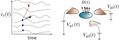
Figure 1: Quantum quenches for electrons in a generic disordered grain. (a) The non-interacting fermions occupy levels of a random Hamiltonian. (b) External time dependent gate voltages and fields move the levels and induce transitions between them. For slow changes, these happen through Landau-Zener transitions between neighboring levels (black arrow in panel (a)), while for faster changes electron-hole excitations between remote levels dominate (red dashed arrow in panel (a)).

Along with this amazing experimental progress, exact fluctuation theorems have been derived and experimentally verified workreview ; jarz ; crooks ; molecule1 ; molecule2 ; batalhao ; pekola ; pekola2 , links between energy transfer (work), Lochschmidt echo, and quantum information scrambling has been established otocGu ; otoc1 ; otocexp ; otocexp2 , and the full distribution of work has been investigated in many-body systems such as Luttinger liquids lutt ; FD ; FD1 ; FD2 ; liebliniger or systems close to quantum criticality gap1 ; gap2 . So far, however, only very few studies investigate the effect of randomness random1 ; random2 ; random3 , playing a crucial role in most nanosystems, and even these studies focus on sudden quenches and do not address quantum statistics and/or interactions.

In this work, we study the properties and universal aspects of quantum work produced in course of time dependent quantum quenches in generic, non-interacting, but disordered fermionic many-body nanosystems. These systems provide an ideal platform to study quantum thermodynamics and the interplay of quantum time evolution, disorder, and quantum statistics.

Generic noninteracting nanosystems obey random matrix statistics matrixreview ; RMreview , and can be described in terms of a Hamiltonian

$$\hat{H}(t)=\sum_{i,j=1}^{N}\hat{a}_{i}^{\dagger}\,\mathcal{H}_{ij}(t)\,\hat{a}_{j}\,,$$ (1)

with the $\hat{a}_{i}$ denoting fermionic annihilation operators, and $\mathcal{H}(t)$ an $N\times N$ random matrix. We assume that the system is in its $M$-particle ground state at time $t=0$, and then work is performed by changing external gate voltages or by applying time dependent magnetic fields mesobook (see Fig. 1). We describe this situation by performing a quench (ramp) at a constant pace, $v\equiv\langle\text{Tr}(\text{d}_{t}{\cal H}^{2})\rangle^{1/2}$, related to the frequency $\omega$ of external parameters, and investigate the distribution of the internal energy injected,

$$P_{t}(W)\equiv\Big{\langle}\Big{\langle}\delta\big{[}W-(\hat{H}(t)-E_{\text{GS}}(t))\big{]}\Big{\rangle}\Big{\rangle}_{\rm RM},$$ (2)

with the two averages referring to quantum and random matrix averages, respectively. Though work and heat cannot be quite disentangled in course of the quench process, throughout this paper we follow the standard practice workreview and refer to this internal energy change – directly related to calorimetric measurements in driven nanosystems calorimetry1 ; calorimetry2 – as work.

Following Ref. wilkinson2 , we apply a quench protocol, $\mathcal{H}(t)=\mathcal{H}_{1}\cos\lambda(t)+\mathcal{H}_{2}\sin\lambda(t)$, with $\dot{\lambda}$ set to constant, and $\mathcal{H}_{1,2}$ independent $N\times N$ matrices, drawn from a Gaussian random matrix ensemble matrixreview ; footnote_J , $\mathcal{P}\left(\mathcal{H}\right)\sim e^{-\beta\frac{N}{4}{\rm Tr}\mathcal{H}^{2}}$. Here we focus on Gaussian orthogonal ($\beta=1$) and Gaussian unitary ($\beta=2$) ensembles, corresponding to integer spin time reversal invariant systems, and systems with broken time reversal symmetry, respectively.

We first construct a determinant formula for the generating function of work in non-interacting fermionic systems. The determinant formula presented can be considered as the dynamical analogue of Anderson’s determinant formula for the orthogonality catastropheAnderson . However, while Anderson restricts himself to the probability of staying in the ground state after a local sudden quench (placing a scatterer at the origin), the determinant formula used here describes the response to any dynamical quench in a non-interacting fermionic many-body system, and describes all possible transitions and the corresponding overlaps.

We find that energy is absorbed by the system via hard core particle diffusion in energy space, and that the statistical properties of work depend crucially on the speed $v$ of the quench as well as on underlying symmetries. For slow, almost adiabatic changes, in particular, $P_{t}(W)$ displays a universal structure, with surprisingly large, superdiffusive work fluctuations, $\langle\delta W^{2}\rangle\sim\langle W\rangle^{3/2}$. Energy absorption at small frequencies, $\omega\sim v$, reflects the symmetry (universality class) of the Hamiltonian and is predicted to scale as, $\langle W\rangle\sim\omega^{1+\beta/2}$, with the random matrix parameter $\beta=1,2$ and $4$ corresponding to orthogonal, unitary, and symplectic symmetries.

The paper is organized as follows. We discuss the time dependent many-body wave function and present a determinant formula for the characteristic function of work in Sec. II. We study the full distribution of work in Sec. III. In Sec. IV we turn to the average work and show that it can be understood in terms of a diffusion in energy space. To shed more light on the dynamics, in Sec. V we show that the most important features of the work statistics can be captured by a classical symmetric exclusion process, and in Sec. VI we also present a simple mean field description allowing the derivation of analytical results. We summarize our main findings in Sec. VII. Technical details of the calculations, as well as additional numerical results for the Gaussian unitary ensemble are relegated to appendices.

II Many-body wave function

To compute the distribution (2), we first need to determine the many-body wave function of our electron system after the quench, $|\Psi(t)\rangle$. To do that, we exploit the fact that our Hamiltonian is non-interacting, and – the initial state of the system being a Slater determinant – the state $|\Psi(t)\rangle$ can also be expressed as a Slater determinant at any time in terms of the time-evolved single particle wave functions. Alternatively, $|\Psi(t)\rangle$ can be written as

$$|\Psi(t)\rangle=\prod_{m=1}^{M}\hat{c}_{m,t}^{\dagger}|0\rangle$$ (3)

with the operators $\hat{c}_{m,t}^{\dagger}$ creating single particles in the states ${\mbox{\boldmath$\varphi$}}^{m}(t)$; $\hat{c}_{m,t}^{\dagger}|0\rangle\equiv|\mbox{\boldmath$\varphi$}^{m}(t)\rangle$. Here the vectors $\mbox{\boldmath$\varphi$}^{m}(t)$ satisfy the single particle Schrödinger equation

$$i\,\partial_{t}\mbox{\boldmath$\varphi$}^{m}(t)={\cal H}(t)\mbox{\boldmath$\varphi$}^{m}(t)$$ (4)

with the boundary conditions $\varphi_{i}^{m}(0)=\delta^{m}_{i}$.

To solve Eq. (4), we use the adiabatic approach. We introduce the instantaneous eigenvectors of ${\cal H}(t)$, $\mbox{\boldmath$\eta$}_{\,t}^{m}$, satisfying ${\cal H}(t)\,\mbox{\boldmath$\eta$}_{\,t}^{m}=\varepsilon_{m}(t)\mbox{\boldmath$\eta$}_{\,t}^{m}$, and corresponding fermionic creation operators, $|\mbox{\boldmath$\eta$}_{\,t}^{m}\rangle\equiv\hat{b}_{m,t}^{\dagger}|0\rangle$. We then expand the $\mbox{\boldmath$\varphi$}^{m}(t)$’s in the instantaneous basis as

$$\mbox{\boldmath$\varphi$}^{m}(t)=\sum_{k}\alpha^{m}_{k}(t)\,\mbox{\boldmath$\eta$}^{k}_{t}\,,$$ (5)

and determine the expansion coefficients by solving the corresponding equation of motion,

$$i\,\dot{\alpha}_{k}(t)=\varepsilon_{k}(t)\alpha_{k}(t)+\sum_{l}A^{kl}(t)\,\alpha_{l}(t)$$ (6)

with $A^{kl}=-i\;\mbox{\boldmath$\eta$}^{k}_{t}\cdot\partial_{t}\mbox{\boldmath$\eta$}^{l}_{t}$ the Berry connection footnoteA (for details of the numerical calculation see Appendix B).

Since $\hat{c}^{\dagger}_{m,t}=\sum_{k}\alpha^{m}_{k}(t)\,\hat{b}^{\dagger}_{k,t}$, knowledge of the coefficients $\alpha^{m}_{k}(t)$ allows us to express the many-body state $|\Psi(t)\rangle$ in the instantaneous basis. Observing furthermore that the many-body Hamiltonian assumes a particularly simple form in the instantaneous basis, $\hat{H}(t)=\sum_{m}\varepsilon_{m}(t)\,\hat{b}_{m,t}^{\dagger}\hat{b}_{m,t}$, we can rewrite the expectation value $\langle\Psi(t)|\,e^{iu\hat{H}(t)}\,|\Psi(t)\rangle$ as

$$\langle\Psi(t)|\,e^{iu\hat{H}(t)}\,|\Psi(t)\rangle= \sum_{\begin{subarray}{c}\{k_{1},k_{2},...,k_{M}\},\\ \{k_{1}^{\prime},k_{2}^{\prime},...,k_{M}^{\prime}\}=1\end{subarray}}^{N}e^{iu\sum_{m=1}^{M}\varepsilon_{k_{m}}(t)}\;\prod_{m=1}^{M}\alpha_{k_{m}}^{m}(t)\left[\alpha_{k_{m}^{\prime}}^{m}(t)\right]^{*}\langle 0|\hat{b}_{k_{1}^{\prime},t}\hat{b}_{k_{2}^{\prime},t}...\hat{b}_{k_{M}^{\prime},t}\hat{b}_{k_{M},t}^{\dagger}...\hat{b}_{k_{2},t}^{\dagger}\hat{b}_{k_{1},t}^{\dagger}|0\rangle.$$ (7)

We can now evaluate the expectation values using Wick’s theorem and eliminate the summation over the labels $\{k_{1}^{\prime},k_{2}^{\prime},...,k_{M}^{\prime}\}$. Transferring furthermore the permutation operators from the lower index of the $\alpha_{k}^{m}$’s to their upper index and reordering sums and products yields

$$\langle e^{iu\hat{H}(t)}\rangle= \sum_{P}(-1)^{P}\prod_{m=1}^{M}\left[g_{t}(u)\right]^{m,Pm}$$ (8)

with $P$ running over all permutations of the $M$ occupied states, and the $M\times M$ matrix $g_{t}(u)$ incorporating all information on the overlap between initial and final single particle states,

$$\left[g_{t}(u)\right]^{mm^{\prime}}\equiv\sum_{k}[\alpha_{k}^{m}(t)]^{*}\,e^{i\,u\,\varepsilon_{k}(t)}\,\alpha_{k}^{m^{\prime}}(t).$$ (9)

This leads immediately to the dererminant formula,

$$G_{t}(u) =\big{\langle}\big{\langle}\Psi(t)|\,e^{iu\left(\hat{H}(t)-E_{\text{GS}}(t)\right)}\,|\Psi(t)\big{\rangle}\big{\rangle}_{\text{RM}}$$

$$=\big{\langle}e^{-i\,u\,\sum_{m=1}^{M}\varepsilon_{m}(t)}\,{\rm det}\,g_{t}(u)\big{\rangle}_{\text{RM}}\,.$$ (10)

Eq. (10) is one of the important results of this work: it establishes a connection between the work statistics of the many-body system and the time evolution of individual single particle states Poster ; FeiQuan . In the following, we shall use this formula to study the properties of quantum quenches in generic fermionic nano-systems described by random matrix theory.

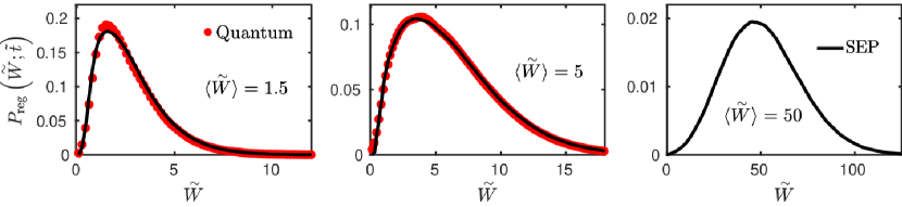
Figure 2: Time evolution of work statistics for the Gaussian orthogonal ensemble in the limit, $\tilde{v}\lesssim 1$. Circles: quantum results for the regular part, $P_{{\rm reg}}(\stackrel{{\scriptstyle\,\sim}}{{\smash{W}\rule{0.0pt}{5.59721pt}}};\tilde{t})$, for dimensionless velocity $\tilde{v}=0.8$ and $N=20$ levels. In the three panels, we used different dimensionless quench times $\tilde{t}=4.88,\,6.25$, and 162.5 (from (a) to (c)), corresponding to dimensionless average work $\langle\stackrel{{\scriptstyle\,\sim}}{{\smash{W}\rule{0.0pt}{5.59721pt}}}\rangle=1.5,\,5$, and 50, respectively footnoteB . Solid lines: SEP simulations. The distribution becomes more and more Gaussian-like as $\langle\stackrel{{\scriptstyle\,\sim}}{{\smash{W}\rule{0.0pt}{5.59721pt}}}\rangle$ increases.

III Quantum statistics of work

To determine the full distribution $P_{t}(W)$, we utilized Eqs. (6) and (10). We generated random matrices ${\cal H}_{1}$ and ${\cal H}_{2}$, determined the expansion coefficients $\alpha^{m}_{k}(t)$ and the determinant ${\rm det}\,g_{t}(u)$ numerically, averaged over the random matrix ensemble, and finally determined $P_{t}(W)$ by taking the Fourier transform of Eq. (10). In our numerical simulations, we focus on the half-filled case, $M=N/2$, though the results are independent of this assumption and carry over to any filling $M/N$. Our results are summarized in Figs. 2 and 3.

The function $P_{t}(W)$ can be disentangled into an adiabatic (ground state) and a regular part as

$$P_{t}(W)=P_{\text{GS}}(t)\,\delta(W)+P_{\rm reg}(W;t).$$ (11)

These functions depend not only on time, but also on the velocity $v$, by which we drag the Hamiltonian through the random matrix manifold, on the position of the Fermi level, and on the symmetry class, too. However, once expressed in terms of appropriate dimensionless quantities, $\stackrel{{\scriptstyle\,\sim}}{{\smash{W}\rule{0.0pt}{5.59721pt}}}\equiv W/{\hbox{\vbox{\hrule height=0.5pt\kern 1.29167pt\hbox{\kern-1.00006pt$\Delta$\kern-1.00006pt}}}}$, $\tilde{t}\equiv t\,\,{\hbox{\vbox{\hrule height=0.5pt\kern 1.29167pt\hbox{\kern-1.00006pt$\Delta$\kern-1.00006pt}}}}$, and $\tilde{v}\equiv{v}/{\hbox{\vbox{\hrule height=0.5pt\kern 1.29167pt\hbox{\kern-1.00006pt$\Delta$\kern-1.00006pt}}}}$, measured in units of the average single particle level spacing  $\Delta$ at the Fermi energy, they become universal functions in the limit $N\to\infty$, $P_{\rm reg}\to P_{\rm reg}(\stackrel{{\scriptstyle\,\sim}}{{\smash{W}\rule{0.0pt}{5.59721pt}}};\tilde{t})$ and $P_{\text{GS}}\to P_{\text{GS}}(\tilde{t})$, displayed in Figs. 2 and 3 for the orthogonal ensemble. They depend implicitly on $\tilde{v}$ but, supposedly, they are independent of all microscopic details, and depend just on the symmetry of the underlying Hamiltonian (see also Appendix C for data for the Gaussian unitary ensemble). Remarkably, these functions simplify even further in the slow quench limit, $\tilde{v}\lesssim 1$, and become functions only of the average work, $\langle\stackrel{{\scriptstyle\,\sim}}{{\smash{W}\rule{0.0pt}{5.59721pt}}}\rangle$, rather than time and velocity. This is demonstrated for the probability of adiabatic transitions in Fig. 3 within the orthogonal ensemble.

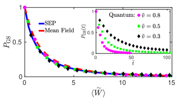
Figure 3: Probability of adiabaticity. Inset: Time evolution of the adiabatic process probability, $P_{{\rm GS}}$, for the orthogonal ensemble ($\beta=1$) for three different velocities, $\tilde{v}\lesssim 1$. Main panel: Symbols: same data as in inset, but plotted as functions of $\langle\stackrel{{\scriptstyle\,\sim}}{{\smash{W}\rule{0.0pt}{5.59721pt}}}\rangle$, collapsing all to a single curve. Solid line: classical SEP result. Dashed line: Eq. (16) obtained by mean field theory.

The functions $P_{\rm reg}(\stackrel{{\scriptstyle\,\sim}}{{\smash{W}\rule{0.0pt}{5.59721pt}}};\tilde{t})$ show a rather slow evolution towards a Gaussian distribution, as we increase $\langle\stackrel{{\scriptstyle\,\sim}}{{\smash{W}\rule{0.0pt}{5.59721pt}}}\rangle.$ As closer numerical investigation reveals, the work fluctuations follow a superdiffusive scaling, ${\delta\!\stackrel{{\scriptstyle\,\sim}}{{\smash{W}\rule{0.0pt}{5.59721pt}}}\!\!{}^{2}\sim\tilde{t}^{\,3/2}\sim\,\stackrel{{\scriptstyle\,\sim}}{{\smash{W}\rule{0.0pt}{5.59721pt}}}\!\!{}^{\,3/2}}$. The behavior of $P_{\text{GS}}(\tilde{t})$ is also somewhat unexpected: the probability of an adiabatic transition is found to decay as a stretched exponential, $P_{\text{GS}}(\tilde{t})\sim{\tilde{t}}^{\,1/4}\,e^{-C\sqrt{\tilde{t}}}$. As we discuss and demonstrate below, both are particular features of a symmetrical exclusion process which governs the dynamics in energy space.

IV Energy space diffusion and average work

Fig. 4 shows the average of the occupation of each level $f_{k}(t)\equiv\langle\langle\hat{n}_{k,t}\rangle\rangle_{\text{RM}}$.footnote_f_k The occupation profile exhibits a clear diffusive character, and is very precisely described by a diffusively broadened Fermi-sea,

$$f_{k}(t)\approx\left[1-{\rm erf}\left(\Delta k/(4\widetilde{D}\tilde{t})^{1/2}\right)\right]/2,$$ (12)

where $\Delta k\equiv k-M$ is the distance of level $k$ from the Fermi energy, and $\widetilde{D}$ denotes a dimensionless diffusion constant in energy space. The diffusive $\sim\sqrt{t}$ broadening of the Fermi surface immediately implies a linear internal energy absorption, $\sim t$,

$$\langle W(t)\rangle\approx{\hbox{\vbox{\hrule height=0.5pt\kern 1.29167pt\hbox{\kern-1.00006pt$\Delta$\kern-1.00006pt}}}}\,\,\widetilde{D}(\tilde{v})\;\tilde{t}\;,$$ (13)

as clearly demonstrated in the inset of Fig. 4. The diffusion constant $\widetilde{D}$ can thus be interpreted as an overall dimensionless energy absorption rate.

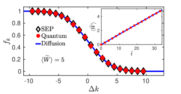
Figure 4: Diffusive broadening of the occupation profile $f_{k}(t)$ for the orthogonal ensemble, plotted as a function of $\Delta k=k-M$, for $\langle\stackrel{{\scriptstyle\,\sim}}{{\smash{W}\rule{0.0pt}{5.59721pt}}}\rangle=5$. Circles: quantum results for a dimensionless velocity $\tilde{v}=0.5$ and $N=20$. Diamonds: SEP simulations. Solid line: diffusive error function fit. Inset: time evolution of dimensionless average work, $\langle\stackrel{{\scriptstyle\,\sim}}{{\smash{W}\rule{0.0pt}{5.59721pt}}}\rangle$ (circles), as a function of the dimensionless time, $\tilde{t}$. Solid line: SEP simulation yielding ${\langle\stackrel{{\scriptstyle\,\sim}}{{\smash{W}\rule{0.0pt}{5.59721pt}}}\rangle\approx\widetilde{D}\,\tilde{t},}$ with a dimensionless diffusion constant $\widetilde{D}=0.145.$

The constant $\widetilde{D}$ depends on the universality class of the system as well as on the velocity, $\tilde{v}$. We can distinguish two distinct regimes: in the “fast limit”, $\tilde{v}\gg 1$, electron-hole transitions between remote levels dominate energy absorption, and we find $\widetilde{D}(\tilde{v})\sim\tilde{v}^{2}\sim\omega^{2}$, as expected in metals. However, in the “slow limit”, $\tilde{v}\lesssim 1$, nearest neighbor transitions mediated by Landau-Zener transitions dominate. The statistics of these latter have been studied thoroughly wilkinson1 ; wilkinson2 ; wilkinsondiff1 , and it has been shown that the parameters of Landau-Zener transitions display universal distributions (see also Appendix A for details). A simple calculation making use of this universal statistics then yields an energy absorption $\widetilde{D}(\tilde{v})\sim\tilde{v}^{1+\beta/2}\sim|\omega|^{1+\beta/2}$ for $\tilde{v}\lesssim 1$, as indeed confirmed by our detailed numerical simulations (see Appendix A).

V Markovian simulation and symmetrical exclusion process

In the slow limit, $\tilde{v}\lesssim 1$, dominated by Landau-Zener transitions, most features of the work statistics can be understood in terms of a simple, classical model, the symmetrical exclusion process (SEP) in energy space. In this approach, we consider the occupation of each level as a classical statistical variable, taking values $n_{k,t}=1$ and 0, and think of Landau-Zener transitions as random, Markovian events, transferring particles between neighboring levels with some probability $p_{\text{LZ}}$. The probabilities $P_{\{n_{k}\}}$ can then be obtained by performing Monte Carlo averaging. First we initialize the fermions on the $M$ lowest levels, then we apply a Markov process in the space of level occupations. During this process, the fermion configuration can only change by nearest neighbor transitions and each such transition happens with rate $\tilde{D}(\tilde{v})$. Note that this model uses a single parameter extracted from the full quantum simulation, the diffusion constant $\tilde{D}(\tilde{v})$ footnoteC . We then determine the work statistics as

$$P_{t}(W)=\Big{\langle}\sum_{\{n_{k}\}}P_{\{n_{k}\}}\,\delta\left[W-\big{(}E_{\{n_{k}\}}(t)-E_{\text{GS}}(t)\big{)}\right]\Big{\rangle}_{\rm RM}$$ (14)

with $E_{\{n_{k}\}}(t)=\sum_{k}\varepsilon_{k}(t)n_{k}(t)$, and the random matrix average performed only on the final eigenenergies, $\varepsilon_{k}(t)$.

As shown in Figs. 2, 3, and 4, apart from the very short time behavior where quantum mechanics rules, the simple SEP approach reproduces the results of our fully quantum mechanical computations with amazing accuracy for slow quenches. This result now allows us to use SEP computations to obtain predictions for the work distribution function in the regime of large injected work, $\langle\stackrel{{\scriptstyle\,\sim}}{{\smash{W}\rule{0.0pt}{5.59721pt}}}\rangle\gtrsim 20$, inaccessible to our quantum mechanical simulations. These results are shown in the rightmost panel of Fig. 2.

VI Mean field description

The SEP model thus provides an accurate description of energy absorption for the most interesting, universal regime, $\tilde{v}\lesssim 1$, but provides limited analytical understanding. We can construct, however, a simple mean field theory of work distribution, by assuming that the occupations $n_{k}$ are classical binary variables with expectation values $f_{k}(t)=\langle n_{k}\rangle$, and that they are independent – apart from overall particle number conservation. This simple mean field theory incorporates three important ingredients: Pauli principle, particle number conservation, and the diffusive character of Fermi surface broadening. Below we demonstrate that this approach can be used to obtain analytical assymptotic estimates for the probability of adiabaticity and for the variance of work.

VI.1 Probability of adiabaticity

Within the mean field approach, we consider each occupation number $n_{k}$ as a binary probability variable, having values $n_{k}=0$ and $1$. In the simplest classical approximation neglecting all correlations between different levels, at time $t$ we can assign the probabilities $f_{k}(t)$ and $1–f_{k}(t)$ to $n_{k}=1$ and $n_{k}=0$, respectively,

$$p_{k,t}(n_{k})=n_{k}\,f_{k}(t)+(1-n_{k})\big{(}1-f_{k}(t)\big{)}\;.$$ (15)

Here we set the expectation value of $n_{k}$, $f_{k}(t)$, in accordance with the diffusively broadened Fermi sea, Eq. (12). To incorporate correlations at the lowest order, we supplement Eq. (15) with a global constraint expressing particle number conservation, $\sum_{k}n_{k}=M$. For simplicity, here we focus on the half-filled case $M\equiv N/2$, though calculations can easily be extended to any value of $M$. We enforce the constraint by inserting a Kronecker $\delta$ function into the joint probability distribution,

$$P\left(\{n_{k}\}\right) =\dfrac{1}{\mathcal{N}_{t}}\prod_{k=1}^{N}p_{k,t}(n_{k})\;\delta_{N/2=\sum_{k}n_{k}}$$

$$=\dfrac{1}{\mathcal{N}_{t}}\int_{-\pi}^{\pi}\dfrac{{\rm d}\lambda}{2\pi}e^{i\lambda\sum_{k=1}^{N}\left(n_{k}-1/2\right)}\prod_{k=1}^{N}p_{k,t}(n_{k})\;.$$

Here ${\mathcal{N}_{t}}$ is a time dependent normalization factor, which can be estimated by first carrying out the summation over $\{n_{k}\}$, and then applying the saddle point approximation as

$$\mathcal{N}_{t} \approx\int_{-\pi}^{\pi}\dfrac{{\rm d}\lambda}{2\pi}\prod_{j>0}\left[\cos^{2}(\lambda/2)+\sin^{2}(\lambda/2)\mathrm{erf}^{2}\left(\frac{j}{\sqrt{4\widetilde{D}\tilde{t}}}\right)\right]$$

$$\approx\left(8\pi\widetilde{D}\tilde{t}\right)^{-1/4}\;.$$

The probability of staying in the ground state then reads

$$P_{\text{GS}} (t)=\dfrac{1}{\mathcal{N}_{t}}\prod_{k=1}^{N/2}f_{k}(t)\prod_{k=N/2+1}^{N}\big{(}1-f_{k}(t)\big{)}$$

$$\approx \dfrac{1}{\mathcal{N}_{t}}e^{2\sqrt{4\widetilde{D}\tilde{t}}\int_{0}^{\infty}\!{\rm d}x\log[(1+\mathrm{erf}(x))/2]}\;.$$

Here, again, an integral approximation has been made by assuming $\widetilde{D}\tilde{t}\approx\;\stackrel{{\scriptstyle\,\sim}}{{\smash{W}\rule{0.0pt}{5.59721pt}}}\,\gg 1$ and the saddle point approximation has been carried out, leading to the asymptotic estimate,

$$P_{\text{GS}}(t)=(8\pi\widetilde{D}\tilde{t})^{1/4}\,e^{-C\sqrt{\widetilde{D}\tilde{t}}}\;,$$ (16)

yielding an excellent fit for $\langle\stackrel{{\scriptstyle\,\sim}}{{\smash{W}\rule{0.0pt}{5.59721pt}}}\rangle>1$, as shown in Fig. 3.

VI.2 Variance of work

For $\stackrel{{\scriptstyle\,\sim}}{{\smash{W}\rule{0.0pt}{5.59721pt}}}\,\gg 1$, we can estimate the variance of the work by neglecting the fluctuations of the individual energy levels vonDelft_KondoBox_paper , $\varepsilon_{k}(t)\to{\hbox{\vbox{\hrule height=0.5pt\kern 1.29167pt\hbox{\kern-1.00006pt$\Delta$\kern-1.00006pt}}}}\,k$, while keeping track of the fluctuations of the occupation numbers. For a given realization of ${\cal H}(t)$, this yields the approximate expression

$$\delta\!\stackrel{{\scriptstyle\,\sim}}{{\smash{W}\rule{0.0pt}{5.59721pt}}}\!\!{}^{2}(t)\approx\Big{\langle}\big{(}\sum_{k=1}^{N}\Delta k\,\hat{n}_{k,t}\big{)}^{2}\Big{\rangle}-\Big{\langle}\sum_{k=1}^{N}\Delta k\,\hat{n}_{k,t}\Big{\rangle}^{2},$$

the average signs denoting here just quantum averages. By separating the ‘diagonal’ contributions, the average $\langle\delta\!\stackrel{{\scriptstyle\,\sim}}{{\smash{W}\rule{0.0pt}{5.59721pt}}}\!\!{}^{2}\rangle_{\rm RM}$ can be rewritten as

$$\langle\delta\!\stackrel{{\scriptstyle\,\sim}}{{\smash{W}\rule{0.0pt}{5.59721pt}}}\!\!{}^{2} (t)\rangle_{\rm RM}\approx\sum_{k}\Delta k^{2}\,\big{\langle}\big{\langle}\delta\hat{n}_{k,t}^{2}\big{\rangle}\big{\rangle}_{\rm RM}$$

$$+\sum_{k\neq k^{\prime}}\Delta k\,\Delta k^{\prime}\big{\langle}\big{\langle}\delta\hat{n}_{k,t}\delta\hat{n}_{k^{\prime},t}\big{\rangle}\big{\rangle}_{\rm RM}$$ (17)

with $\delta\hat{n}_{k,t}\equiv\hat{n}_{k,t}-\langle\hat{n}_{k,t}\rangle$ denoting the deviation of the occupation number. Since the $\hat{n}_{k,t}$ behave as binary variables, averages in the first term can be expressed as $\langle\langle\delta\hat{n}_{k,t}^{2}\rangle\rangle_{\rm RM}=f_{k}(t)\big{(}1-f_{k}(t)\big{)}$, with $f_{k}\left(t\right)\approx\big{(}1-{\rm erf}(\Delta k/\sqrt{4\widetilde{D}\tilde{t}}\,)\big{)}/2$. The correlators appearing in this equation can be expressed in terms of the amplitudes $\alpha^{m}(t)$ as $\langle\delta\hat{n}_{k,t}\delta\hat{n}_{k^{\prime},t}\rangle=-\big{|}\sum_{m=1}^{N/2}{\alpha_{k}^{m}(t)}^{*}\alpha_{k^{\prime}}^{m}(t)\big{|}^{2}$. Notice that this correction is negative, indicating that the level occupations are anticorrelated, as dictated by particle number conservation.

By neglecting for a moment these correlations and replacing sums by integrals, we obtain the estimate

$$\langle\delta\!\stackrel{{\scriptstyle\,\sim}}{{\smash{W}\rule{0.0pt}{5.59721pt}}}\!\!{}^{2}(t)\rangle_{\rm RM}\approx\int_{-\infty}^{\infty}{\rm d}x\,x^{2}\,\frac{1-{\rm erf}^{2}(x/\sqrt{4\widetilde{D}\tilde{t}})}{4}\sim\tilde{t}^{3/2}\,,$$

reproducing the superdiffusive scaling $\langle\delta\!\!\stackrel{{\scriptstyle\,\sim}}{{\smash{W}\rule{0.0pt}{5.59721pt}}}\!\!{}^{2}\rangle\sim\langle\stackrel{{\scriptstyle\,\sim}}{{\smash{W}\rule{0.0pt}{5.59721pt}}}\rangle^{3/2}$. We note that while neglecting the correlations explains the observed behavior of the work’s variance, it does not reproduce the correct prefactor. Indeed, a more careful mean field calculation along the lines of the previous subsection showsMF that correlations (the conservation of fermion number) cannot be entirely neglected, and they also give a similar but smaller $\sim\tilde{t}^{3/2}$ contribution to the variance – without changing the overall scaling.

VII Conclusions

We have derived and used a determinant formula to compute the distribution of work, $P_{t}(W)$, in course of a quantum quench in generic, disordered, fermionic nano-systems, and have shown that it displays a large degree of universality, especially in the slow quench limit. Even if a complete experimental characterization of $P_{t}(W)$ may still be challenging, many of our curious findings such as the diffusive broadening of the Fermi energy, the $\sim t^{3/2}$ scaling of the variance of the energy absorbed, or the low frequency $\sim\omega^{1+\beta/2}$ absorption rate, could be readily verified experimentally.

Our results also demonstrate that quantum work statistics in these systems is, after all, to a large extent classical. In the most interesting slow quench limit, we demonstrate a close connection to the symmetrical exclusion process (SEP), a classical diffusion of hard core particles in energy space. Quantum mechanics enters here through level collisions, giving rise to Landau-Zener transitions, the exclusion process, mirroring the Pauli principle and, finally, level statistics, reflecting the symmetry of the underlying quantum mechanical system.

Though diffusion in energy space and its relation to thermalization has been studied by several authors in different contextswilkinsondiff1 ; JarzynskiPRE1993 ; CohenPRL2013 , earlier works have not focused on the impact of quantum statistics on energy diffusion. In particular, here we find that energy absorption in this many-body system corresponds to diffusion of strongly interacting particles. This very strong interaction, captured at the classical level by the exclusion process, implies that while the total energy absorbed shows a clear drift in time, $\langle W\rangle\sim t$, its spread is non-diffusive but rather increases superdiffusively as $\langle\delta W^{2}\rangle\sim t^{3/2}$ during a quench.

Our investigations, focusing on $T=0$ temperature non-interacting systems, represent clearly only the first step. Inclusion of interactions, generalizations to the symplectic universality class as well as to finite temperatures and open systems are all exciting open questions for future research.

Appendix A Statistics of avoided level crossing

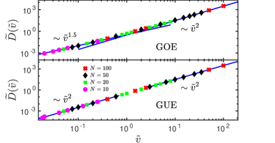
Figure 5: Universality of diffusion constants. Dimensionless diffusion constants plotted as the function of the dimensionless velocity of the quench, $\tilde{v}$, for (a) GOE and (b) GUE, using different matrix sizes $N$, with logarithmic scale on both axes. The data trace out a universal curve, scaling as $\widetilde{D}\sim\tilde{v}^{1+\beta/2}$ in the slow quench limit, $\tilde{v}\lesssim 1$. For fast quenches, $\tilde{v}\gg 1$, the statistical aspects of level repulsion lose their role and no longer govern the many-body dynamics, leading to $\widetilde{D}\sim\tilde{v}^{2}$ for both ensembles.

At small velocities, $\tilde{v}\lesssim 1$, Landau-Zener transitions dominate the energy absorption process. The statistical properties of these transitions are universal wilkinson3 ; wilkinsondiff2 and depend on the particular universality class considered. In practice, we consider motions within the random matrix manyfold along a ‘circle’,

$$\mathcal{H}(\lambda)=\mathcal{H}_{1}\cos\lambda+\mathcal{H}_{2}\sin\lambda,$$ (18)

and investigate the separation of neighboring levels, $\Delta(\lambda)\equiv\varepsilon_{k+1}(\lambda)-\varepsilon_{k}(\lambda)$. This function displays well-defined minima, $\Delta_{\rm min}$, at positions $\lambda_{0}$, close to which the level separation can be well-described in terms of an effective two-level Hamiltonian as

$$\Delta(\lambda)\approx\sqrt{\Delta_{\rm min}^{2}+\gamma^{2}(\lambda-\lambda_{0})^{2}}.$$ (19)

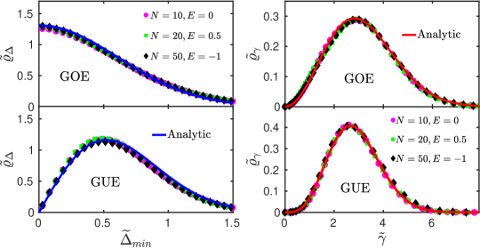
Figure 6: Universality of distribution of avoided level crossing parameters for the (a)-(b) Gaussian orthogonal (GOE) and (c)-(d) Gaussian unitary ensembles (GUE). (a),(c) The dimensionless Landau-Zener gap ${\widetilde{\Delta}}_{\text{min}}$, and (b),(d) slopes $\tilde{\gamma}$ display universal distributions, depending only on the symmetry class of $\cal H$, independent of its size, $N$, and the energy, $E$. Notice that $\tilde{\varrho}_{\Delta}({\widetilde{\Delta}}_{\text{min}})\sim{\widetilde{\Delta}}_{\text{min}}^{\beta-1}$, implying $\tilde{\varrho}_{\Delta}(0)=\text{finite}$ for GOE, $\beta=1$, and a breakdown of the adiabatic limit. Continuous lines denote analytical results of Refs. wilkinson3 ; wilkinsondiff2 .

The number of level crossings occurring between two selected neighboring levels is directly proportional to the distance covered within the random matrix manifold, $N_{\rm cross}\sim s_{\text{tot}}\sim\sqrt{N}\,{\rm d}\lambda$. Therefore, we can define the probability distribution of $\Delta_{\rm min}$ as

$${\rm d}N_{\rm cross}=\rho(\Delta_{\rm min})\,{\rm d}s\,{\rm d}\Delta_{\rm min}\;.$$ (20)

Here the density function $\rho(\Delta_{\rm min})$ depends implicitly on the size of the random matrices, $N$, as well as on the universality class considered footnoterho . The dependence on $N$, however, appears just in a trivial way in the large $N$ limit, through the level spacing  $\Delta$ at the energy of the Landau-Zener transitions. This dependence can be scaled out, yielding a universal distribution function,

$$\tilde{\varrho}(\widetilde{\Delta}_{\rm min})\equiv{{\hbox{\vbox{\hrule height=0.5pt\kern 1.29167pt\hbox{\kern-1.00006pt$\Delta$\kern-1.00006pt}}}}}\,\,{\rho}\left({\Delta}_{\rm min}\right),$$ (21)

with $\widetilde{\Delta}_{\rm min}=\Delta_{\rm min}/{\hbox{\vbox{\hrule height=0.5pt\kern 1.29167pt\hbox{\kern-1.00006pt$\Delta$\kern-1.00006pt}}}}$ denoting the dimensionless Landau-Zener gap.

Similarly, the distribution of the slopes $\gamma$ is also universal, provided we measure it in its natural unit,

$$\tilde{\gamma}=\gamma\sqrt{N}.$$

The numerically computed statistics of the distributions $\tilde{\varrho}(\widetilde{\Delta}_{\rm min})$ and $\tilde{\varrho}(\tilde{\gamma})$ are displayed for the Gaussian orthogonal ensemble (GOE, $\beta=1$) and Gaussian unitary ensemble (GUE, $\beta=2$) in Fig. 6. The numerically extracted distributions fit perfectly the analytical predictions of Ref. wilkinson3, . In particular, the distribution of the slopes has a peaked structure, i.e., there exist a typical value of $\tilde{\gamma}$, characterizing the transitions.

The distribution $\tilde{\varrho}(\widetilde{\Delta}_{\rm min})$ is, on the other hand, more peculiar. In particular, $\tilde{\varrho}(\widetilde{\Delta}_{\rm min})\sim\Delta_{\rm min}^{\beta-1}$, and scales as

$$\tilde{\varrho}(\widetilde{\Delta}_{\rm min}\ll 1)\approx\begin{cases}\pi^{3/2}/\sqrt{18}&\text{for $\beta=1$, }\\ {2\,\pi^{3/2}}\,\,\widetilde{\Delta}_{\rm min}/3&\text{for $\beta=2$, }\end{cases}$$

in the orthogonal and unitary universality classes, investigated here in detail footnote_pi . This curious behavior implies that avoided level crossings with very small gap are abundant in the orthogonal class, which leads to a breakdown of adiabatic perturbation theory for $\beta=1$.

The probability $p_{\rm LZ}$ of a Landau-Zener transition between two neighboring levels depends on the velocity at which the transition is approached, and is known analytically LZ1 ; LZ2 ,

$$p_{\rm LZ}=\exp\left(-\dfrac{\pi^{2}}{2}\dfrac{\widetilde{\Delta}_{\rm min}^{2}}{\tilde{v}\,\tilde{\gamma}}\right)\,.$$ (22)

Given the exponential sensitivity to $\Delta_{\rm min}$, small Landau-Zener gap transitions dominate in the limit of small velocities, $\tilde{v}\ll 1$. This leads to the estimate

$$\widetilde{D} \sim\big{\langle}{\rm d}_{t}N_{\rm cross}\,\,p_{\rm LZ}\big{\rangle}=\tilde{v}\int{\rm d}\widetilde{\Delta}_{\rm min}\,\tilde{\varrho}_{\beta}(\widetilde{\Delta}_{\rm min})\,\langle p_{\rm LZ}\rangle_{\gamma}$$

$$\sim\tilde{v}^{1+\beta/2}.$$ (23)

Figure 7: Comparison of the regular part of the work statistics, $P_{\rm reg}(\stackrel{{\scriptstyle\,\sim}}{{\smash{W}\rule{0.0pt}{5.59721pt}}};\tilde{t})$ for (a)-(c) the orthogonal (GOE) and (d)-(f) the unitary matrix ensembles (GUE), with $\stackrel{{\scriptstyle\,\sim}}{{\smash{W}\rule{0.0pt}{5.59721pt}}}$ and $\tilde{t}$ referring to dimensionless work and time. Symbols: regular part for different values of the dimensionless average work, $\langle\stackrel{{\scriptstyle\,\sim}}{{\smash{W}\rule{0.0pt}{5.59721pt}}}\rangle=1.5$, $3$, and $5$, and a dimensionless quench velocity, $\tilde{v}=0.8$, for two different matrix sizes, $N=20$ and $N=50$. The distributions show universal behavior and collapse into a single curve independent of the system size, $N$. Arrows indicate the positions of the first neighboring levels at $\stackrel{{\scriptstyle\,\sim}}{{\smash{W}\rule{0.0pt}{5.59721pt}}}=1,2,...$. Solid lines: classical SEP simulations provide an excellent approximation for $\tilde{v}\lesssim 1$. In this limit, $P_{\rm reg}(\stackrel{{\scriptstyle\,\sim}}{{\smash{W}\rule{0.0pt}{5.59721pt}}};\tilde{t})$ depends only the average dimensionless work, $\langle\stackrel{{\scriptstyle\,\sim}}{{\smash{W}\rule{0.0pt}{5.59721pt}}}\rangle$, for both ensembles.

The universal scaling of the many-body diffusion constant, as extracted from our simulations, is plotted in Fig. 5. For time reversal symmetry breaking (unitary) systems, the diffusion constant scales both at small and high velocities as ${\tilde{v}}^{2}$. In the orthogonal case, however, a clear crossover is demonstrated between a Landau-Zener dominated small velocity regime with $\widetilde{D}\sim{\tilde{v}}^{3/2}$, and a high velocity fast quench regime with $\widetilde{D}\sim\tilde{v}^{2}$ .

Appendix B Time evolution of single particle states

To solve Eq. (6) in the main text, it is practical to make a simple gauge transformation, and eliminate the phase dependence generated by the instantaneous eigenenergy, $\varepsilon_{k}(t)$,

$$\alpha_{k}(t)\equiv e^{-i\Theta_{k}(t)}\tilde{\alpha}_{k}(t)\,$$

with the dynamical phase defined as

$$\Theta_{k}(t)=\int_{0}^{t}dt^{\prime}\varepsilon_{k}(t^{\prime}).$$ (24)

Importantly, dynamical phases cancel in the expression of the occupation numbers, $f_{k}(t)$, as well in the expression of the work and its generating function. Therefore, in all these equations, we can just replace $\alpha_{k}(t)$ by $\tilde{\alpha}_{k}(t)$, obeying the simpler differential equation,

$$i\,\dot{\tilde{\alpha}}_{k}(t)=\sum_{l}A^{kl}(t)\,\tilde{\alpha}_{l}(t)\,.$$ (25)

In practical calculations, it is useful to avoid numerical differentiation, and calculate the Berry connection as

$$A^{kl}(t)=-i\,\langle\mbox{\boldmath$\eta$}^{k}_{t}|\partial_{t}\mbox{\boldmath$\eta$}^{l}_{t}\rangle=i\,\dfrac{\mbox{\boldmath$\eta$}^{k}_{t}\cdot\partial_{t}{\cal H}(t)\,{\mbox{\boldmath$\eta$}}^{l}_{t}}{\varepsilon_{k}(t)-\varepsilon_{l}(t)}.$$ (26)

In our numerics, we made use of the fourth order Runge-Kutta method to solve the single particle time-dependent Schrödinger equation. Dynamical phases in Eq. (24) were determined numerically using the Simpson-formula. Since the phases of the instantaneous states often make jumps, we enforced the choice ${A_{kk}=-i\;{\mbox{\boldmath$\eta$}}^{k}_{t}\cdot\partial_{t}{\mbox{\boldmath$\eta$}}^{k}_{t}=0}$ by requiring that the overlaps of two consecutive eigenstates remain close to 1, $\langle\mbox{\boldmath$\eta$}^{k}_{t}|\mbox{\boldmath$\eta$}^{k}_{t+\delta t}\rangle\approx 1$.

Appendix C Fingerprints of level repulsion and deviations from universality

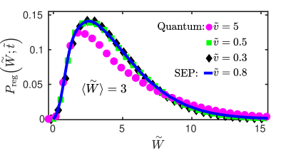
Figure 8: Universality of the distribution $P_{\rm reg}(\stackrel{{\scriptstyle\,\sim}}{{\smash{W}\rule{0.0pt}{5.59721pt}}};\tilde{t})$ in the limit $\tilde{v}\lesssim 1$ for the orthogonal ensemble. Symbols: quantum results for $N=20$ levels and $\tilde{v}=0.3$, $\tilde{v}=0.5$, and $\tilde{v}=5$. Solid line: classical SEP result for $\tilde{v}=0.8$. While all $\tilde{v}\lesssim 1$ results fall on top of each other for the same amount of average work, for $\tilde{v}=5$, deviations appear due to transitions between non nearest neighbor levels.

As discussed in the main text, the distribution of the work is universal, i.e., it is independent from the system size $N$ as well as the Fermi energy; it depends solely on the dimensionless time, the dimensionless velocity, and the symmetry class of the random Hamiltonians. This is illustrated in Fig. 7, where we have fixed the dimensionless quench velocity to $\tilde{v}=0.8$, and the dimensionless times such that they correspond to an injected dimensionless work $\langle\stackrel{{\scriptstyle\,\sim}}{{\smash{W}\rule{0.0pt}{5.59721pt}}}\rangle=1.5$, $3$, and $5$ in both symmetry classes.

For relatively small injected internal energies, $W\lesssim 5\;{\hbox{\vbox{\hrule height=0.5pt\kern 1.29167pt\hbox{\kern-1.00006pt$\Delta$\kern-1.00006pt}}}}$, the discreteness of the energy levels becomes apparent, and fingerprints of level repulsion can be observed. First, $P(\stackrel{{\scriptstyle\,\sim}}{{\smash{W}\rule{0.0pt}{5.59721pt}}})$ vanishes continuously at zero (within SEP as $\stackrel{{\scriptstyle\,\sim}}{{\smash{W}\rule{0.0pt}{5.59721pt}}}\!\!{}^{\beta}$), since the first empty level is repelled from the last occupied level. Moreover, additional wiggles appear in $P(\stackrel{{\scriptstyle\,\sim}}{{\smash{W}\rule{0.0pt}{5.59721pt}}})$, reflecting the positions of first, second and third neighbors. These features are more pronounced in the Gaussian unitary ensemble, where level repulsions are stronger, and are expected to become even more pronounced for the symplectic ensemble, not studied here. The observed distributions are, however, independent of the matrix size, $N$, as stated above.

Remarkably, even for $\tilde{v}=0.8$, SEP simulations (continuous lines in Fig. 7) provide an almost perfect description of the full quantum results. For larger velocities, however, deviations occur. This is demonstrated in Fig. 8. Clearly, for $\tilde{v}\gtrsim 1$ the role of Landau-Zener transitions is reduced, the SEP description loses its validity, and distributions depend explicitly on the velocity $\tilde{v}$.

References

- (1) P. Talkner, E. Lutz, and P. Hänggi, Phys. Rev. E 75, 050102(R) (2007).
- (2) M. Campisi, P. Hänggi, and P. Talkner, Rev. Mod. Phys. 83, 771 (2011).
- (3) A. Alemany, M. Ribezzi, and F. Ritort, AIP Conf. Proc. 1332, 96 (2011).
- (4) J. Liphardt, S. Dumont, S. B. Smith, I. Tinoco Jr., C. Bustamante, Science 96, 1833 (2002).
- (5) D. Collin, F. Ritort, C. Jarzynski, S. B. Smith, I. Tinoco Jr., and C. Bustamante, Nature 437, 231 (2005).
- (6) T. B. Batalhão, A. M. Souza, L. Mazzola, R. Auccaise, R. S. Sarthour, I. S. Oliveira, J. Goold, G. De Chiara, M. Paternostro, and R. M. Serra, Phys. Rev. Lett. 113, 140601 (2014).
- (7) O.-P. Saira, Y. Yoon, T. Tanttu, M. Möttönen, D. V. Averin, and J. P. Pekola, Phys. Rev. Lett. 109, 180601 (2012).
- (8) J. V. Koski and J. P. Pekola, in: Binder F., Correa L., Gogolin C., Anders J., Adesso G. (eds), Thermodynamics in the Quantum Regime, Fundamental Theories of Physics, vol 195. Springer, Cham
- (9) C. Jarzynski, Phys. Rev. Lett. 78, 2690 (1997).
- (10) G. E. Crooks, Phys. Rev. E 60, 2721 (1999).
- (11) P. W. Anderson, Phys. Rev. Lett. Review Letters. 18, 1049 (1967).
- (12) M. Campisi and J. Goold, Phys. Rev. E 95, 062127 (2017).
- (13) A. Kitaev, talk at Fundamental Physics Prize Symposium Nov. 10, 2014.
- (14) M. Gärttner, J. G. Bohnet, A. Safavi-Naini, M. L. Wall, J. J. Bollinger, and A. M. Rey, Nat. Phys. 13, 781 (2017).
- (15) J. Li, R. Fan, H. Wang, B. Ye, B. Zeng, H. Zhai, X. Peng, and J. Du, Phys. Rev. X 7, 031011 (2017).
- (16) B. Dóra, Á. Bácsi, and G. Zaránd, Phys. Rev. B 86, 161109(R) (2012).
- (17) S. Dorosz, T. Platini, and D. Karevski, Phys. Rev. E 77, 051120 (2008).
- (18) J. Yi, P. Talkner, and M. Campisi, Phys. Rev. E 84, 011138 (2011).
- (19) J. Yi, Y. W. Kim, and P. Talkner, Phys. Rev. E 85, 051107 (2012).
- (20) G. Perfetto, L. Piroli, and A. Gambassi, Phys. Rev. E 100, 032114 (2019).
- (21) A. Silva, Phys. Rev. Lett. 101, 120603 (2008).
- (22) A. Gambassi, and A. Silva, Phys. Rev. Lett. 109, 250602 (2012).
- (23) M. Łobejko, J. Łuczka, and P. Talkner, Phys. Rev. E 95, 052137 (2017).
- (24) E. G. Arrais, D. A. Wisniacki, L. C. Céleri, N. G. de Almeida, A. J. Roncaglia, and F. Toscano, Phys. Rev. E 98, 012106 (2018).
- (25) A. Chenu, J. Molina-Vilaplana, and A. del Campo, Quantum 3, 127 (2019).
- (26) C. W. J. Beenakker, Rev. Mod. Phys. 69, 731 (1997).
- (27) T. Guhr, A. Müller-Groeling, and H. A. Weidenmüller, Phys. Rep. 299, 189 (1998).
- (28) Y. Imry, Introduction to Mesoscopic Physics, (Oxford University Press, Oxford, 2002).
- (29) S. Gasparinetti, K. L. Viisanen, O. P. Saira, T. Faivre, M. Arzeo, M. Meschke, and J.P. Pekola, Phys. Rev. Applied 3, 014007 (2015).
- (30) E. D. Walsh, D. K. Efetov, G.-H. Lee, M. Heuck, J. Crossno, T. A. Ohki, P. Kim, D. Englund, and K. C. Fong, Phys. Rev. Applied 8, 024022 (2017).
- (31) P. N. Walker, M. J. Sánchez, and M. Wilkinson, J. Math. Phys. 37, 5019 (1996).
- (32) For simplicity, we set the usual energy unit to here.
- (33) We fix the gauge of the vectors such that at any time.
- (34) I. Lovas, A. Grabarits, and G. Zaránd, Theory of heat statistics in nanograins, invited contribution at Frontiers of Quantum and Mesoscopic Thermodynamics 2019, July 2019, Prague.
- (35) A similar determinant formula has been derived in a parallel work, Z. Fei and H. T. Quan, arXiv:1909.10350v2.
- (36) We used typically samples to generate the work statistics.
- (37) This quantity can be computed without the determinant formula as .
- (38) M. Wilkinson, J. Phys. A: Math. Gen. 21, 4021 (1988).
- (39) I. Tikhonenkov, A. Vardi, J. R. Anglin, and D. Cohen Phys. Rev. Lett. 110, 050401 (2013).
- (40) C. Jarzynski, Phys. Rev. E 48, 4340 (1993).
- (41) A. Grabarits et al, unpublished.
- (42) M. Wilkinson and E. J. Austin, Phys. Rev. A 47, 2601 (1993).
- (43) We have also set up a slightly more complicated classical Markovian process to model the dynamics. Here we performed a Monte Carlo averaging over the matrices and ; for each pair we again intialized the fermions at the lowest levels. We then looked at the spectrum of , and each time we encountered a Landau-Zener crossing such that only one of the two colliding levels was occupied, the fermion hopped to the other level with the Landau-Zener transition probability calculated for the particular level crossing. We have checked that this process yielded results very similar to the simplified version presented in the main text.
- (44) P. N. Walker, M. J. Sánchez, and M. Wilkinson, J. Math. Phys. 37, 5019 (1996).
- (45) M. Wilkinson, J. Phys. A: Math. Gen. 21, 4021 (1988).
- (46) More generally, the density of avoided level crossings between any two neighboring levels depends also on the energy of the colliding levels, . By concentrating on the middle of the spectrum, here we restrict our analysis to energy .
- (47) Our convention differs from the one used in Ref. wilkinson3, , where is measured in units , leading to a factor of difference in the density .
- (48) L. Landau, Phys. Z. Sowj. 2, 46 (1932).
- (49) C. Zener, Proc. R. Soc. 137, 696 (1932).
- (50) W. B. Thimm, J. Kroha, and J. von Delft, Phys. Rev. Lett. 82, 2143 (1999).