The linear stability of Reissner-Nordström spacetime:
the full subextremal range $|Q|<M$

Abstract

We prove the linear stability of subextremal Reissner-Nordström spacetimes as solutions to the Einstein–Maxwell equation. We make use of a novel representation of gauge-invariant quantities which satisfy a symmetric system of coupled wave equations. This system is composed of two of the three equations derived in our previous works Giorgi4 , Giorgi5 , where the estimates required arbitrary smallness of the charge. Here, the estimates are obtained by defining a combined energy-momentum tensor for the system in terms of the symmetric structure of the right hand sides of the equations. We obtain boundedness of the energy, Morawetz estimates and decay for the full subextremal range $|Q|<M$, completely in physical space. Such decay estimates, together with the estimates for the gauge-dependent quantities of the perturbations obtained in Giorgi6 , settle the problem of linear stability to gravitational and electromagnetic perturbations of Reissner-Nordström solution in the full subextremal range $|Q|<M$.

1 Introduction

The problem of stability of black holes as solutions to the Einstein equation occupies a central stage in mathematical General Relativity Ch . The resolution of this problem consists in understanding the long-time dynamics of perturbations of known stationary solutions to the Einstein equation.

There are few examples of exact solutions to the Einstein equation, the most fundamental of which is the Kerr spacetime kerr , axially symmetric and stationary solution to the Einstein vacuum equation

$$\operatorname{Ric}(g)=0,$$

where $g$ is a Lorentzian metric in $3+1$-dimensions. A particular case of the Kerr spacetime is the Schwarzschild solution Schwarz , which is spherically symmetric and static, given in coordinates $(t,r,\theta,\phi)$ by

$$g_{M} = -\left(1-\frac{2M}{r}\right)dt^{2}+\left(1-\frac{2M}{r}\right)^{-1}dr^{2}+r^{2}\left(d\theta^{2}+\sin^{2}\theta d\phi^{2}\right).$$

The parameter $M$ can be interpreted as the mass of the black hole.

In the case of the Einstein equation coupled with electromagnetic fields, the Lorentzian metric $g$ satisfies the Einstein–Maxwell equation Chandra , i.e.

$$\operatorname{Ric}(g)_{\mu\nu} = 2F_{\mu\lambda}{F_{\nu}}^{\lambda}-\frac{1}{2}g_{\mu\nu}F^{\alpha\beta}F_{\alpha\beta},$$ (1)

$$D_{[\alpha}F_{\beta\gamma]} = 0,\qquad D^{\alpha}F_{\alpha\beta}=0,$$ (2)

where $F$ is a two-form verifying the Maxwell equations (2), and $D$ is the Levi-Civita connection of $g$. In this context, the fundamental stationary and axisymmetric solution is the Kerr–Newman spacetime Newman , and its spherically symmetric and static case is given by the Reissner–Nordström metric Nordstrom , given in coordinates by

$$g_{M,Q} = -\left(1-\frac{2M}{r}+\frac{Q^{2}}{r^{2}}\right)dt^{2}+\left(1-\frac{2M}{r}+\frac{Q^{2}}{r^{2}}\right)^{-1}dr^{2}+r^{2}\left(d\theta^{2}+\sin^{2}\theta d\phi^{2}\right).$$ (3)

The parameter $Q$ can be interpreted as the charge of the black hole for $|Q|<M$, which is referred to as the subextremal range. The case $|Q|=M$ is called the extremal case, while $|Q|>M$ corresponds to a spacetime with naked singularities. Observe that for $Q=0$, the Reissner-Nordström metric (3) reduces to the Schwarzschild one.

The problem of stability of black hole solutions can be roughly divided into three formulations, each of increasing difficulty, from the formal mode analysis of the linearized equations to the fully non-linear perturbations, passing through the problem of linear stability.

The mode stability consists in formally separating the solutions to the linearized Einstein equation into modes at fixed frequencies, and aims at proving the lack of exponentially growing modes for all metric or curvature components. The study of the mode stability of the Schwarzschild solution was initiated by Regge, Wheeler Regge-Wheeler and Zerilli Zerilli in metric perturbations (in which the metric of the solution is perturbed), and by Barden and Press Bardeen-Press in Newman–Penrose formalism (in which the curvature of the solution, through the Newman–Penrose scalars, is perturbed). See also Dotti Dotti . Chandrasekhar Chandra identified a transformation theory in mode decomposition which connects the two approaches in Schwarzschild, which is now referred to as Chandrasekhar transformation. Teukolsky Teukolsky extended the equations in Newman-Penrose formalism to the Kerr spacetime, and Whiting Whiting proved the mode stability for Kerr spacetime. The study of mode stability of the Reissner-Nordström spacetime has been initiated by Moncrief Moncrief1 , Moncrief2 , Moncrief3 , who obtained the wave equations governing the perturbations in metric perturbations. Chandrasekhar Chandra1 , Chandra-RN2 completed the study of the fixed mode perturbations in Newman–Penrose formalism. See also Fernández Tío–Dotti Dotti2 .

This weak version of stability is however not sufficient to prove boundedness and decay of the solutions even to the linearized equations. Indeed, the lack of exponentially growing modes is still consistent with the statement that general perturbations with finite initial energy grow unboundedly in time, because results at the level of individual modes do not imply them for the superposition of infinitely many modes lectures .

The resolution of the problem of linear stability consists in proving boundedness and decay for the solutions to the linearized Einstein equation, which does not rely on decomposition in modes but rather on a physical space analysis. The stability of the Schwarzschild solution to the linearized Einstein vacuum equation has been obtained by Dafermos–Holzegel–Rodnianski DHR by using curvature perturbations and analysis of the Teukolsky equation. The authors introduced a physical-space version of the Chandrasekhar transformation and crucially used the extensive progress on boundedness and decay results for wave equations on black hole backgrounds (for instance redshift , rp , lectures ). Other proofs have followed: see Hung–Keller–Wang mu-tao for the proof of the linear stability using metric perturbations, through the analysis of Regge–Wheeler and Zerilli equations. See also Hung pei-ken , pei-ken-2 for a proof in the harmonic gauge and Johnson Johnson2 in the generalized harmonic gauge. There have been numerous recent results for the linear stability of Kerr spacetime. Quantitative decay estimates for the Teukolsky equation in slowly rotating Kerr spacetime have been obtained by Ma ma2 and Dafermos–Holzegel–Rodnianski TeukolskyDHR . Andersson–Bäckdahl–Blue–Ma Kerr-lin1 used the outgoing gauge and Häfner–Hintz–Vasy Kerr-lin2 used the wave gauge to prove linear stability of Kerr with small angular momentum. Decay for solutions to the Maxwell equations in Schwarzschild spacetime have been obtained by Blue BlueMax and Pasqualotto Federico .

The ultimate goal of the problem of stability is the study of the dynamics of perturbations of solutions to the fully non-linear Einstein equation. The fully non-linear stability of the Kerr(-Newman) family consists in showing that a small perturbation of a Kerr(-Newman) spacetime which is a solution to the non-linear Einstein(-Maxwell) equation converges to another member of the Kerr(-Newman) family. The only proof of non-linear stability with no symmetry assumptions which is known at this stage, in the asymptotically flat regime, is the global non-linear stability of Minkowski spacetime by Christodolou-Klainerman Ch-Kl , which was followed by proofs obtained through different approaches (see Zipser , Lind-Rod , Hintz-Vasy-M ). See also Zipser Zipser for the proof of non-linear stability of Minkowski as solution to the Einstein–Maxwell equation. The first proof of non-linear stability of the Schwarzschild spacetime under the class of symmetry of axially symmetric polarized perturbations was given by Klainerman–Szeftel stabilitySchwarzschild . In the presence of a positive cosmological constant, the Kerr–de Sitter and the Kerr–Newman–de Sitter family with small angular momentum have been proved to be non-linearly stable by Hintz–Vasy Hintz-Vasy and by Hintz Hintz-M respectively.

In this paper we solve the problem of linear stability of the Reissner–Nordström spacetime (3) as solution to the linearized Einstein–Maxwell equations (1) and (2), in the full subextremal range $|Q|<M$. More precisely, we prove boundedness and decay statements for solutions to the linearization of the Einstein–Maxwell equation around a Reissner-Nordström solution, and the analysis is carried out completely in physical space. Here is a rough version of our main theorem.

Theorem 1.1

[Linear stability of Reissner-Nordström spacetime to gravitational and electromagnetic perturbations for $|Q|<M$ (Rough version)] All solutions to the linearized Einstein–Maxwell equations around a Reissner–Nordström solution $g_{M,Q}$ for $|Q|<M$ in a certain choice of gauge arising from regular asymptotically flat initial data remain uniformly bounded on the exterior and decay to a linearized Kerr–Newman solution.

Theorem 1.1 represents the final step of a program that was initiated by the author in Giorgi4 , Giorgi5 and Giorgi6 to prove the linear stability of Reissner-Nordström spacetime to gravitational and electromagnetic perturbations in the full subextremal range. More precisely, the series of works Giorgi4 , Giorgi5 and Giorgi6 amounted to the proof of the linear stability in the case of arbitrarily small charge $|Q|\ll M$. The main result of this paper is to extend the control of all components of the perturbation to the subextremal range $|Q|<M$.

Remark 1

The subextremal range $|Q|<M$ for which the linear stability holds is expected to be optimal. The estimates as hereby derived make use of the redshift vector field at the horizon, and therefore they are degenerate through the extremal case limit $|Q|=M$. In particular, the same decay estimates obtained in Giorgi6 are not expected to hold in the extremal case due to the Aretakis instability extremal-1 , extremal-2 . Such instability causes the growth of transversal derivatives along the horizon of solutions to the non-linear wave equation extremal-3 , and it is expected that this phenomenon persists in the linearized gravity. Nevertheless, some weaker version of stability, which takes into account such degeneracy of transversal derivative along the event horizon, could hold in the extremal case, where stability and instability phenomena concur.

In what follows, we recall the main ideas from the series of works Giorgi4 , Giorgi5 and Giorgi6 . They consist in two parts:

• The main system of three wave equations governing the perturbations are derived and analyzed for arbitrarily small charge in Giorgi4 and Giorgi5 . More precisely, two wave equations of spin $\pm 2$ (governing the gravitational perturbations) are obtained in Giorgi4 , and one wave equation of spin $\pm 1$ (governing the electromagnetic radiations) is obtained in Giorgi5 . Those are wave equations for quantities which are invariant to coordinate transformations at linear level, which we call gauge-invariant quantities.

• The above analysis is used in Giorgi6 to obtain control for all the components of the perturbations, upon a choice of gauge. In particular, the estimates for the gauge-invariant quantities are used to obtain estimates for the gauge-dependent ones.

In the present paper, we will make use in a fundamental way of the system of equations obtained in Giorgi4 and Giorgi5 , and derive from them a new system to obtain control for the gauge-invariant quantities in the full subextremal range. The result in Giorgi6 will then be applied straightforwardly to obtain control for the gauge-dependent quantities from the new estimates obtained here for the gauge-invariant ones.

We now recall the main results in Giorgi4 , Giorgi5 and Giorgi6 which are particularly relevant for this work.

1.1 The spin $\pm 2$ system of equations in Giorgi4

Suppose that $({\mathcal{M}},g,F)$ is a solution to the Einstein–Maxwell equation such that the manifold ${\mathcal{M}}$ can be foliated by $2$-spheres $S$. In Giorgi4 , we defined the symmetric traceless $2$-covariant $S$-tensors $\alpha$ and $\mathfrak{f}$ defined relative to a null frame $\{e_{3},e_{4},e_{A}\}_{A=1,2}$ as

$$\alpha_{AB} = W(e_{4},e_{A},e_{4},e_{B}),\qquad\mathfrak{f}_{AB}=\,{\mathcal{D}}{\,{}^{\star}\mkern-2.0mu}\mkern-16.0mu/_{2}\,^{(F)}\beta_{AB}+\,^{(F)}\rho\widehat{\chi}_{AB}$$

where $W$ is the Weyl curvature, $\,{\mathcal{D}}{\,{}^{\star}\mkern-2.0mu}\mkern-16.0mu/_{2}\,^{(F)}\beta_{AB}=-D_{(A}\,^{(F)}\beta_{B)}+\frac{1}{2}g_{AB}\mbox{div}\mkern-19.0mu/\,\,\,\,\,^{(F)}\beta$ with $D$ the Levi-Civita connection of $g$, $\,{}^{(F)}\beta_{A}=F(e_{A},e_{4})$, $\,{}^{(F)}\rho=\frac{1}{2}F(e_{3},e_{4})$ and $\widehat{\chi}$ is the traceless part of the $S$-tensor $\chi_{AB}=g(D_{A}e_{4},e_{B})$.

The 2-tensors $\alpha$ and $\mathfrak{f}$ are gauge-invariant, and satisfy a coupled system of Teukolsky-type equations of spin $\pm 2$ Giorgi4 . The estimates for the Teukolsky equations cannot be obtained directly, but rather through a Chandrasekhar transformation to obtain Regge–Wheeler-type equations. We defined the derived quantities $\mathfrak{q}$ and $\mathfrak{q}^{\bf F}$ Giorgi4

$$\mathfrak{q} =\frac{1}{\underline{\kappa}}\nabla\mkern-13.0mu/\,_{3}\left(\frac{r}{\underline{\kappa}}\nabla\mkern-13.0mu/\,_{3}(r^{3}\underline{\kappa}^{2}\alpha)\right),\qquad\mathfrak{q}^{\bf F}=\frac{1}{\underline{\kappa}}\nabla\mkern-13.0mu/\,_{3}(r^{3}\underline{\kappa}\ \mathfrak{f})$$

where $\underline{\kappa}:=\mbox{tr}\underline{\chi}$ is the trace of the second null fundamental form and $\nabla\mkern-13.0mu/\,_{3}$ is the projection of the sphere of the covariant derivative along the incoming null direction $D_{e_{3}}$.

The gauge-invariant 2-tensors $\mathfrak{q}$ and $\mathfrak{q}^{\bf F}$ satisfy a coupled system of linear wave equations of spin $\pm 2$ Giorgi4 which can be schematically written as

$$\Box_{g_{M,Q}}\mathfrak{q}+\tilde{V}_{1}(r)\ \mathfrak{q} = Q\cdot\Big{(}b_{1}(r)\mbox{$\bigtriangleup\mkern-13.0mu/\,$}_{2}\mathfrak{q}^{\bf F}+b_{2}(r)\partial_{r}\mathfrak{q}^{\bf F}+b_{3}(r)\mathfrak{q}^{\bf F}+\mbox{l.o.t.}\Big{)}$$ (4)

$$\Box_{g_{M,Q}}\mathfrak{q}^{\bf F}+\tilde{V}_{2}(r)\ \mathfrak{q}^{\bf F} = Q\cdot\left(c_{1}(r)\mathfrak{q}+\mbox{l.o.t.}\right)$$ (5)

where $\Box_{g_{M,Q}}$ is the d’Alembertian of the Reissner–Nordström metric $g_{M,Q}$ applied to 2-tensors, $b_{i}$, $c_{i}$, $\tilde{V}_{i}$ are smooth functions of an area radius function $r$, $\mbox{$\bigtriangleup\mkern-13.0mu/\,$}_{2}$ denotes the Laplacian operator on 2-tensors on the sphere and l.o.t. denotes lower order terms (with respect to differentiability) for $\mathfrak{q}$ and $\mathfrak{q}^{\bf F}$.

Estimates for this system are obtained in Giorgi4 in the case of $|Q|\ll M$ by interpreting the right hand sides of (4) and (5) as a perturbation of zero. A careful analysis has to be done at the trapping region in order to absorb the spacetime integrals obtained from the right hand side, but the arbitrary smallness of the charge allows to absorb them into the bulk energies of the left hand side of the equations. Through transport estimates, one can then obtain control for the quantities $\mathfrak{f}$ and $\alpha$. We refer to Giorgi4 for more details.

Observe that the first of the equations, i.e. equation (4), reduces to the Regge–Wheeler equation used in DHR in the case of Schwarzschild (with trivial right hand side).

1.2 The spin $\pm 1$ equation in Giorgi5

In Giorgi5 , we defined the 1-covariant $S$-tensor $\tilde{\beta}$ relative to a null frame $\{e_{3},e_{4},e_{A}\}_{A=1,2}$ as

$$\tilde{\beta}_{A}:=2\,^{(F)}\rho\beta_{A}-3\rho\,^{(F)}\beta_{A}$$

where $\,{}^{(F)}\beta_{A}=F(e_{A},e_{4})$, $\,{}^{(F)}\rho=\frac{1}{2}F(e_{3},e_{4})$, $\beta_{A}=\frac{1}{2}W(e_{A},e_{4},e_{3},e_{4})$, $\rho=\frac{1}{4}W(e_{3},e_{4},e_{3},e_{4})$.

The 1-tensor $\tilde{\beta}$ is a mixed curvature-electromagnetic component which is gauge-invariant and satisfies a Teukolsky-type equation of spin $\pm 1$ Giorgi5 . Also in this case, to obtain the estimates for this equation a Chandrasekhar transformation is applied. We defined the derived quantity $\mathfrak{p}$ Giorgi5

$$\mathfrak{p} =\frac{1}{\underline{\kappa}}\nabla\mkern-13.0mu/\,_{3}(r^{5}\underline{\kappa}\ \tilde{\beta})$$

which is shown to satisfy a linear wave equation of spin $\pm 1$ Giorgi5 which can be schematically written as

$$\Box_{g_{M,Q}}\mathfrak{p}+V_{1}(r)\ \mathfrak{p} = Q\cdot a_{1}(r)\mbox{div}\mkern-19.0mu/\,\,\,\,\mathfrak{q}^{\bf F}$$ (6)

where $a_{1}$ and $V_{1}$ are smooth functions $r$ and $\mbox{div}\mkern-19.0mu/\,\,\,\,$ is the divergence of a symmetric traceless $2$-tensor on the sphere. Observe that equation (6) is coupled to equation (5) through the presence of $\mathfrak{q}^{\bf F}$.

Estimates for this equation are obtained in Giorgi5 in the case of $|Q|\ll M$ by using the control of $\mathfrak{q}^{\bf F}$ previously obtained in Giorgi4 . By decomposing the 1-tensors $\mathfrak{p}$ and $\mbox{div}\mkern-19.0mu/\,\,\,\,\mathfrak{q}^{\bf F}$ in spherical harmonics and projecting equation (6) to the $\ell=1$ harmonics, the right hand side vanishes, and the equation decouples to a single wave equation for the projection of $\mathfrak{p}$ to the $\ell=1$ mode. Standard techniques for decay of wave equations on black hole backgrounds can then be applied to control $\mathfrak{p}_{\ell=1}$, and by transport estimates $\tilde{\beta}_{\ell=1}$. The higher spherical harmonics of $\tilde{\beta}$ are controlled by using a relation between the three quantities of the schematic form Giorgi5 :

$$Q\cdot\nabla\mkern-13.0mu/\,_{3}\alpha = d_{1}(r)\mathfrak{f}+d_{2}(r)\,{\mathcal{D}}{\,{}^{\star}\mkern-2.0mu}\mkern-16.0mu/_{2}\tilde{\beta}$$ (7)

where $d_{i}$ are smooth functions of $r$. We refer to Giorgi5 for more details.

1.3 The proof of linear stability for small charge in Giorgi6

The conclusions of Giorgi4 and Giorgi5 are the pointwise estimates for the gauge-invariant quantities $\mathfrak{q}$, $\mathfrak{q}^{\bf F}$ and $\mathfrak{p}$ for $|Q|\ll M$, and those are the starting point of Giorgi6 , where such estimates are used to obtain control for all the remaining components of the perturbation. Since the remaining components are gauge-dependent, a careful choice of gauge is needed to show that $\mathfrak{q}$, $\mathfrak{q}^{\bf F}$ and $\mathfrak{p}$ control the components of the perturbation, and that in addition their decay is optimal and consistent with non-linear applications.

In Giorgi6 , we achieve such a proof with the choice of outgoing null geodesic, or Bondi, gauge. In this gauge, we made use of residual gauge freedom to define normalizations of scalar functions which allow to obtain integrable transport estimates. We obtain a hierarchy of transport estimates with right hand sides in terms of the known $\mathfrak{q}$, $\mathfrak{q}^{\bf F}$ and $\mathfrak{p}$. By integrating along null hypersurfaces, pointwise estimates for all the remaining components can be obtained from the estimates previously obtained for $\mathfrak{q}$, $\mathfrak{q}^{\bf F}$ and $\mathfrak{p}$ Giorgi6 .

In particular, observe that the estimates for the gauge-dependent quantities in Giorgi6 do not make use of the smallness of the charge once the gauge-invariant quantities are controlled. Since the estimates for $\mathfrak{q}$, $\mathfrak{q}^{\bf F}$ and $\mathfrak{p}$ in Giorgi4 and Giorgi5 are only valid for $|Q|\ll M$, the final proof of the linear stability of Reissner-Nordström in Giorgi6 only holds for arbitrarily small charge. We refer to Giorgi6 for more details.

We stress here that, if one were able to extend the pointwise estimates for $\mathfrak{q}$, $\mathfrak{q}^{\bf F}$ and $\mathfrak{p}$ to the full subextremal range $|Q|<M$, it would be straightforward to apply the proof of linear stability in Giorgi6 , which does not use smallness of the charge, to the full subextremal range. More precisely, the results on boundedness and decay for the gauge-invariant quantities in Section 8.5 of Giorgi6 could be upgraded to hold for $|Q|<M$, and therefore the subsequent control on the gauge-dependent quantities in the following sections of Giorgi6 would also hold in the full subextremal range.

1.4 The mixed spin $\pm 1$ and spin $\pm 2$ system of equations

We outline here the main ideas which allow us to extend the result of linear stability of Reissner-Nordström spacetime from very small charge $|Q|\ll M$ (Giorgi4 , Giorgi5 , Giorgi6 ) to the full subextremal range $|Q|<M$. The fundamental step is to introduce a system, which we denote mixed spin $\pm 1$ and spin $\pm 2$ Regge–Wheeler system, which governs the gravitational and electromagnetic perturbations of the Reissner-Nordström solution and has a symmetric structure, which is favorable in the derivation of the estimates.

We briefly explain how such a system is obtained from the previously mentioned equations appeared in Giorgi4 and Giorgi5 .

Recall the relation (7) between $\nabla\mkern-13.0mu/\,_{3}\alpha$, $\mathfrak{f}$ and $\tilde{\beta}$. By taking one derivative in the $\nabla\mkern-13.0mu/\,_{3}$ direction, one derives a relation between $\mathfrak{q}$, $\mathfrak{q}^{\bf F}$ and $\mathfrak{f}$ of the schematic form (see (31) for the exact expression):

$$Q\cdot\mathfrak{q}=d_{1}(r)\mathfrak{q}^{\bf F}+d_{2}(r)\,{\mathcal{D}}{\,{}^{\star}\mkern-2.0mu}\mkern-16.0mu/_{2}\mathfrak{p}+\mbox{l.o.t.}$$ (8)

Since equations (4), (5), (6) for $\mathfrak{q}$, $\mathfrak{q}^{\bf F}$ and $\mathfrak{p}$ are three wave equations for three quantities which are related through the identity (8), it is clear that the above system of three equations is equivalent to a system of two equations, which is to say that one of the equations is redundant. We therefore look for a system of two equations which is equivalent to the system of three equations (4), (5), (6).

Since $\mathfrak{q}$ and $\mathfrak{q}^{\bf F}$ are $2$-tensors and $\mathfrak{p}$ is a $1$-tensor on the sphere, neglecting equation (6) for $\mathfrak{p}$ would cause the absence of control of the projection to the $\ell=1$ spherical mode of the perturbations. For this reason, we decide to neglect one of the first two equations, more precisely (4), the equation for $\mathfrak{q}$, which has the most intricate right hand side.

We then substitute $\mathfrak{q}$ through the relation (8) into the wave equation (5), and we obtain schematically

$$\Box_{g_{M,Q}}\mathfrak{q}^{\bf F}+\tilde{V}_{2}(r)\ \mathfrak{q}^{\bf F} = c_{1}(r)\left(Q\cdot\mathfrak{q}+\mbox{l.o.t.}\right)$$

$$= c_{1}(r)\left(d_{1}(r)\mathfrak{q}^{\bf F}+d_{2}(r)\,{\mathcal{D}}{\,{}^{\star}\mkern-2.0mu}\mkern-16.0mu/_{2}\mathfrak{p}\right)$$

where the lower order terms, denoted l.o.t. cancel out in the above substitution (see Section 3 for the precise derivation). One then obtains

$$\Box_{g_{M,Q}}\mathfrak{q}^{\bf F}+V_{2}(r)\ \mathfrak{q}^{\bf F} = a_{2}(r)\,{\mathcal{D}}{\,{}^{\star}\mkern-2.0mu}\mkern-16.0mu/_{2}\mathfrak{p}$$ (9)

for a new potential $V_{2}$ and a smooth function $a_{2}$. Observe that equation (9) is now coupled to equation (6). By combining the above wave equations of spin $\pm 2$ and spin $\pm 1$ we obtain a system of two coupled linear wave equations of the following schematic form:

$$\begin{cases}&\Box_{g_{M,Q}}\mathfrak{p}+V_{1}(r)\ \mathfrak{p}=Q\cdot a_{1}(r)\mbox{div}\mkern-19.0mu/\,\,\,\,\mathfrak{q}^{\bf F}\\ &\Box_{g_{M,Q}}\mathfrak{q}^{\bf F}+V_{2}(r)\ \mathfrak{q}^{\bf F}=a_{2}(r)\,{\mathcal{D}}{\,{}^{\star}\mkern-2.0mu}\mkern-16.0mu/_{2}\mathfrak{p}\end{cases}$$

We call the above system the mixed spin $\pm 1$ and spin $\pm 2$ Regge–Wheeler system. Observe that since $\mathfrak{q}$ is related to $\mathfrak{p}$ and $\mathfrak{q}^{\bf F}$ through the relation (8), the above system is equivalent to the system of three equations obtained in Giorgi4 and Giorgi5 . The two quantities $\mathfrak{q}^{\bf F}$ and $\mathfrak{p}$ therefore play the role of gravitational and electromagnetic radiation respectively for perturbations of Reissner–Nordström spacetime.

The fundamental advantage of the derived system compared to the previous one is in its symmetry: the operators $\,{\mathcal{D}}{\,{}^{\star}\mkern-2.0mu}\mkern-16.0mu/_{2}$ and $\mbox{div}\mkern-19.0mu/\,\,\,\,$ appearing on the right hand sides are adjoint operators on the sphere DHR . Such symmetry is used here to define a combined energy-momentum tensor which allows for a cancellation of the highest order terms, without recurring to smallness of the charge. We are therefore able to deduce boundedness of the energy, Morawetz and $r^{p}$-estimates in the full subextremal range $|Q|<M$. This is in contrast with the system analyzed in Giorgi4 , which has non symmetric right hand sides, and for which the analysis can be obtained for very small $Q$ only.

Remark 2

A similar structure in the coupling terms of a system of two wave equations has been found by Hung pei-ken , for odd perturbations of linearized gravity of Schwarzschild in harmonic gauge. In pei-ken , two metric components, denoted $H_{1}$ and $H_{2}$, satisfy a system of wave equations which are coupled through adjoint operators on the sphere, similarly to our mixed spin $\pm 1$ and spin $\pm 2$ Regge–Wheeler system. Hung obtains estimates for the system through a novel definition of energy-momentum tensor which makes use of the symmetric right hand side. We take a similar approach through the definition of a combined energy-momentum tensor as explained below.

1.5 The combined energy-momentum tensor

We now give a brief summary of the proof of boundedness and decay statements for the mixed spin $\pm 1$ and spin $\pm 2$ Regge–Wheeler system.

We define a combined energy-momentum tensor for the system, which takes into account both equations and their structure. Such combined energy-momentum tensor ${\mathcal{T}}_{\mu\nu}[\mathfrak{q}^{\bf F},\mathfrak{p}]$ is tailored on the specific structure of right hand side of the system. More precisely, it consists of the sum of the energy-momentum tensor associated to each equation, plus a mixed term defined in terms of the right hand side. Schematically:

$${\mathcal{T}}_{\mu\nu}[\mathfrak{q}^{\bf F},\mathfrak{p}] := {\mathcal{T}}_{\mu\nu}[\mathfrak{q}^{\bf F}]+{\mathcal{T}}_{\mu\nu}[\mathfrak{p}]-Q\cdot a(r)\left(\,{\mathcal{D}}{\,{}^{\star}\mkern-2.0mu}\mkern-16.0mu/_{2}\mathfrak{p}\cdot\mathfrak{q}^{\bf F}\right)g_{\mu\nu}$$

where ${\mathcal{T}}_{\mu\nu}[\mathfrak{q}^{\bf F}]$ and ${\mathcal{T}}_{\mu\nu}[\mathfrak{p}]$ are the standard energy-momentum tensor associated to the wave equations for $\mathfrak{q}^{\bf F}$ and $\mathfrak{p}$ respectively. See Definition 2 for the exact expression.

Such definition of ${\mathcal{T}}_{\mu\nu}[\mathfrak{q}^{\bf F},\mathfrak{p}]$ is motivated by the following property: when applied with multiplier $X=\partial_{t}$, the associated current ${\mathcal{P}}^{X}_{\mu}={\mathcal{T}}_{\mu\nu}[\mathfrak{q}^{\bf F},\mathfrak{p}]X^{\nu}$ is divergence free. In particular, the additional term $-Q\cdot a(r)\left(\,{\mathcal{D}}{\,{}^{\star}\mkern-2.0mu}\mkern-16.0mu/_{2}\mathfrak{p}\cdot\mathfrak{q}^{\bf F}\right)g_{\mu\nu}$ in the definition of the combined energy-momentum tensor is precisely the one needed to obtain cancellation of the divergence. By applying the divergence theorem to a causal domain, one only needs to prove the positivity of the modified boundary terms to obtain boundedness of the energy, which can be obtained in the full subextremal range $|Q|<M$. This is done in Section 6.

The derivation of Morawetz estimates is more subtle since the divergence of the current associated to $Y=f(r)\partial_{r}$ does not vanish, but has to be proved to be positive definite. Because of the mixed term in the definition of ${\mathcal{T}}_{\mu\nu}[\mathfrak{q}^{\bf F},\mathfrak{p}]$, we obtain a spacetime integral containing terms of the schematic form

$$c_{1}(r)|\mathfrak{q}^{\bf F}|^{2}+c_{2}(r)|\mathfrak{p}|^{2}-c_{3}(r)\left(\mathfrak{q}^{\bf F}\cdot\mathfrak{p}\right)$$

which has to be proved to be positive definite for a well-chosen function $f(r)$. The negativity of the discriminant of the above quadratic form ($D=c_{3}(r)^{2}-4c_{1}(r)c_{2}(r)$), together with the positivity of the coefficients $c_{1}(r)$ and $c_{2}(r)$, is used to conclude that a spacetime integral of the above schematic form is positive definite. This is done in Section 7.

Finally, the $r$-weights appearing on the right hand side of the equations in the mixed spin $\pm 1$ and spin $\pm 2$ Regge–Wheeler system are sufficiently good so that the derivation of the $r^{p}$-hierarchy of Dafermos–Rodnianski for the system is identical to the standard wave equation. This is done in Section 8.

A rough version of the result is as follows. For the precise version, see Theorem 4.1.

Theorem 1.2

[Rough version] Solutions to the mixed spin $\pm 1$ and spin $\pm 2$ Regge–Wheeler system on Reissner-Nordström spacetime with $|Q|<M$ arising from initial data which is prescribed on a Cauchy hypersurface $\Sigma_{0}$ satisfy statements of energy boundedness, integrated local energy decay, and a hierarchy of $r$-weighted energy estimates.

The hierarchy of $r$-weighted estimates is such that, using a pigeonhole principle rp , one obtains in the full subextremal range $|Q|<M$, the pointwise decay estimates

$$|\mathfrak{p}|\leq C\tau^{-1+\delta},\qquad|\mathfrak{q}^{\bf F}|\leq C\tau^{-1+\delta}$$

for $\delta>0$ and a time function $\tau$, where $C$ is some constant depending on an appropriate Sobolev norm of the data.

The pointwise estimates for $\mathfrak{p}$ and $\mathfrak{q}^{\bf F}$ imply estimates for $\mathfrak{q}$ in the full subextremal range through the relation (8). We are then in the condition of having extended the estimates for $\mathfrak{q}$, $\mathfrak{q}^{\bf F}$ and $\mathfrak{p}$ to the full subextremal range $|Q|<M$, and therefore the proof of linear stability Giorgi6 can be applied to obtain control of all the remaining gauge-dependent quantities, as explained in Section 1.3.

The paper is organized as follows. In Section 2 we recall the main properties of Reissner-Nordström spacetime and in Section 3, the symmetric system used in this paper is derived from the equations obtained in Giorgi4 and Giorgi5 . In Section 4, the energy quantities are defined and the main theorem is stated. The energy-momentum tensor associated to the system is defined in Section 5. In Section 6, boundedness of the energy for the full subextremal range $|Q|<M$ is proved. Morawetz estimates for the subextremal range $|Q|<M$ are obtained in Section 7 and the $r^{p}$-estimates are derived in Section 8.

2 The Reissner-Nordström spacetime

In this section, we introduce the Reissner-Nordström exterior metric, as well as relevant background structure. We mostly highlight the properties which are needed in this paper. For a more complete description of the Reissner-Nordström spacetime see Exact .

2.1 The manifold and the metric

Define the manifold with boundary

$$\mathcal{M}:=\mathcal{D}\times S^{2}:=\left(-\infty,0\right]\times\left(0,\infty\right)\times S^{2}$$ (10)

with Kruskal coordinates $\left(U,V,\theta^{1},\theta^{2}\right)$, as defined in Section 3 of Giorgi4 . The boundary $\mathcal{H}^{+}$ will be referred to as the horizon. We denote by $S^{2}_{U,V}$ the $2$-sphere $\left\{U,V\right\}\times S^{2}\subset\mathcal{M}$ in $\mathcal{M}$.

Fix two parameters $M>0$ and $Q$, verifying $|Q|<M$. Then the Reissner-Nordström metric $g_{M,Q}$ with parameters $M$ and $Q$ is defined to be the metric:

$$g_{M,Q}=-4\Upsilon_{K}\left(U,V\right)d{U}d{V}+r^{2}\left(U,V\right)\gamma_{AB}d{\theta}^{A}d{\theta}^{B}.$$ (11)

where

$$\Upsilon_{K}\left(U,V\right) = \frac{r_{-}r_{+}}{4r(U,V)^{2}}\Big{(}\frac{r(U,V)-r_{-}}{r_{-}}\Big{)}^{1+\left(\frac{r_{-}}{r_{+}}\right)^{2}}\exp\Big{(}-\frac{r_{+}-r_{-}}{r_{+}^{2}}r(U,V)\Big{)}$$

$$\gamma_{AB} = \textrm{standard metric on $S^{2}$}\,.$$

and

$$r_{\pm}=M\pm\sqrt{M^{2}-Q^{2}}$$ (12)

and $r$ is an implicit function of the coordinates $U$ and $V$. We denote $r_{\mathcal{H}}=r_{+}=M+\sqrt{M^{2}-Q^{2}}$.

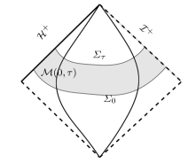
Figure 1: Penrose diagram of the patch covered by the $U$ and $V$ coordinates.

The Kruskal coordinates cover the entire exterior region up to the horizon. We now define another double null coordinate system that covers the interior of $\mathcal{M}$ (up to the event horizon), modulo the degeneration of the angular coordinates. This coordinate system, $\left(u,v,\theta^{1},\theta^{2}\right)$, is called double null coordinates and are defined via the relations

$$U=-\frac{2r_{+}^{2}}{r_{+}-r_{-}}\exp\left(-\frac{r_{+}-r_{-}}{4r_{+}^{2}}u\right)\ \ \ \textrm{and}\ \ \ \ V=\frac{2r_{+}^{2}}{r_{+}-r_{-}}\exp\left(\frac{r_{+}-r_{-}}{4r_{+}^{2}}v\right)\,.$$ (13)

Using (13), we obtain the Reissner-Nordström metric on the interior of ${\mathcal{M}}$ in $\left(u,v,\theta^{1},\theta^{2}\right)$-coordinates:

$$g_{M,Q}=-4\Upsilon\left(u,v\right)\,d{u}\,d{v}+r^{2}\left(u,v\right)\gamma_{AB}d{\theta}^{A}d{\theta}^{B}$$ (14)

with

$$\Upsilon:=1-\frac{2M}{r}+\frac{Q^{2}}{r^{2}}$$ (15)

We denote by $S_{u,v}$ the sphere $S^{2}_{U,V}$ where $U$ and $V$ are given by (13).

Note that $u,v$ are regular optical functions. Their corresponding null geodesic generators are

$${\underline{L}}:=-g^{ab}\partial_{a}v\partial_{b}=\frac{1}{\Upsilon}\partial_{u},\qquad L:=-g^{ab}\partial_{a}u\partial_{b}=\frac{1}{\Upsilon}\partial_{v},$$ (16)

The null frame $(e_{3}^{*},e_{4}^{*})$ for which $e_{3}$ is geodesic (which is regular towards the future along the event horizon) is given by

$$e_{3}^{*}={\underline{L}},\,\,\qquad e_{4}^{*}=\Upsilon L.$$ (17)

The null frame $(e_{3},e_{4})$ for which $e_{4}$ is geodesic (which is regular towards null infinity) is given by

$$e_{3}=\Upsilon{\underline{L}},\,\,\qquad e_{4}=L$$ (18)

The photon sphere of Reissner-Nordstrom corresponds to the hypersurface in which null geodesics are trapped. It is the hypersurface given by $\{r=r_{P}\}$ where $r_{P}$ is the largest root of the polynomial $r^{2}-3Mr+2Q^{2}$, and is given by

$$r_{P}=\frac{3M+\sqrt{9M^{2}-8Q^{2}}}{2}$$ (19)

The curvature and electromagnetic components which are non-vanishing are given by

$$\begin{split}\,{}^{(F)}\rho&=\frac{1}{2}F(e_{3},e_{4})=\frac{Q}{r^{2}},\\ \rho&=\frac{1}{4}W(e_{3},e_{4},e_{3},e_{4})=-\frac{2M}{r^{3}}+\frac{2Q^{2}}{r^{4}}\end{split}$$ (20)

where $F$ is the electromagnetic tensor and $W$ is the Weyl curvature of the Reissner-Nordström solution.

2.2 The Killing vector fields

We define the vectorfield $T$ to be the timelike Killing vector field $\partial_{t}$ of the $(t,r)$ coordinates in (3), which in double null coordinates is given by

$$T=\frac{1}{2}(\partial_{u}+\partial_{v})=\frac{1}{2}(\Upsilon e_{3}^{*}+e_{4}^{*})=\frac{1}{2}(e_{3}+\Upsilon e_{4})$$

We can also define a basis of angular momentum operator $\Omega_{i}$, $i=1,2,3$ (see for example DHR ). The Lie algebra of Killing vector fields of $g_{M,Q}$ is then generated by $T$ and $\Omega_{i}$, for $i=1,2,3$.

2.3 The spherical harmonics and elliptic estimates

We collect some known definitions and properties of the Hodge decomposition of scalars, one forms and symmetric traceless two tensors in spherical harmonics. We also recall some known elliptic estimates. See Section 4.4 of DHR for more details.

We denote by $Y_{m}^{\ell}$, with $|m|\leq\ell$, the spherical harmonics on the sphere of radius $r$, i.e.

$$\mbox{$\bigtriangleup\mkern-13.0mu/\,$}_{0}Y^{\ell}_{m}=-\frac{1}{r^{2}}\ell(\ell+1)Y^{\ell}_{m}$$ (21)

where $\mbox{$\bigtriangleup\mkern-13.0mu/\,$}_{0}$ denotes the laplacian on the sphere $S_{u,v}$ of radius $r=r(u,v)$ for scalar functions.

Definition 1

We say that a function $f$ on $\mathcal{M}$ is supported on $\ell\geq 2$ if the projections

$$\int_{S_{u,v}}f\cdot Y^{\ell}_{m}=0$$

vanish for $Y_{m}^{\ell=1}$ for $m=-1,0,1$.

We recall the following angular operators on $S_{u,v}$-tensors. Let $\xi$ be an arbitrary one-form and $\theta$ an arbitrary symmetric traceless $2$-tensor on $S_{u,v}$.

• $\nabla\mkern-13.0mu/\,$ denotes the covariant derivative associated to the metric $\not{g}$ on $S_{u,v}$.

• $\,{\mathcal{D}}\mkern-8.0mu/_{1}$ takes $\xi$ into the pair of functions $(\mbox{div}\mkern-19.0mu/\,\,\,\,\xi,\mbox{curl}\mkern-19.0mu/\,\,\,\,\xi)$, where

  $$\mbox{div}\mkern-19.0mu/\,\,\,\,\xi=\not{g}^{AB}\nabla\mkern-13.0mu/\,_{A}\xi_{B},\qquad\mbox{curl}\mkern-19.0mu/\,\,\,\,\xi=\not{\epsilon}^{AB}\nabla\mkern-13.0mu/\,_{A}\xi_{B}$$

• $\,{\mathcal{D}}{\,{}^{\star}\mkern-2.0mu}\mkern-16.0mu/_{1}$ is the formal $L^{2}$-adjoint of $\,{\mathcal{D}}\mkern-8.0mu/_{1}$, and takes any pair of functions $(\rho,\sigma)$ into the one-form $-\nabla\mkern-13.0mu/\,_{A}\rho+\not{\epsilon}_{AB}\nabla\mkern-13.0mu/\,^{B}\sigma$.

• $\,{\mathcal{D}}\mkern-8.0mu/_{2}$ takes $\theta$ into the one-form $\,{\mathcal{D}}\mkern-8.0mu/_{2}\theta=(\mbox{div}\mkern-19.0mu/\,\,\,\,\theta)_{C}=\not{g}^{AB}\nabla\mkern-13.0mu/\,_{A}\theta_{BC}$.

• $\,{\mathcal{D}}{\,{}^{\star}\mkern-2.0mu}\mkern-16.0mu/_{2}$ is the formal $L^{2}$-adjoint of $\,{\mathcal{D}}\mkern-8.0mu/_{2}$, and takes $\xi$ into the symmetric traceless two tensor

  $$(\,{\mathcal{D}}{\,{}^{\star}\mkern-2.0mu}\mkern-16.0mu/_{2}\xi)_{AB}=-\frac{1}{2}\left(\nabla\mkern-13.0mu/\,_{B}\xi_{A}+\nabla\mkern-13.0mu/\,_{A}\xi_{B}-(\mbox{div}\mkern-19.0mu/\,\,\,\,\xi)\not{g}_{AB}\right)$$

We can easily check that $\,{\mathcal{D}}{\,{}^{\star}\mkern-2.0mu}\mkern-16.0mu/_{k}$ is the formal adjoint of $\,{\mathcal{D}}\mkern-8.0mu/_{k}$, i.e.

$$\int_{S}(\,{\mathcal{D}}\mkern-8.0mu/_{k}f)g=\int_{S}f(\,{\mathcal{D}}{\,{}^{\star}\mkern-2.0mu}\mkern-16.0mu/_{k}g)$$ (22)

Recall that an arbitrary one-form $\xi$ on $S_{u,v}$ has a unique representation $\xi=r\,{\mathcal{D}}{\,{}^{\star}\mkern-2.0mu}\mkern-16.0mu/_{1}(f,g)$, where $\,{\mathcal{D}}{\,{}^{\star}\mkern-2.0mu}\mkern-16.0mu/_{1}(f,g)$, for two uniquely defined functions $f$ and $g$ on the unit sphere, both with vanishing mean. In particular, the scalars $\mbox{div}\mkern-19.0mu/\,\,\,\,\xi$ and $\mbox{curl}\mkern-19.0mu/\,\,\,\,\xi$ are supported in $\ell\geq 1$.

Recall that an arbitrary symmetric traceless two-tensor $\theta$ on $S_{u,v}$ has a unique representation $\theta=r^{2}\,{\mathcal{D}}{\,{}^{\star}\mkern-2.0mu}\mkern-16.0mu/_{2}\,{\mathcal{D}}{\,{}^{\star}\mkern-2.0mu}\mkern-16.0mu/_{1}(f,g)$ for two uniquely defined functions $f$ and $g$ on the unit sphere, both supported in $\ell\geq 2$. In particular, the scalars $\mbox{div}\mkern-19.0mu/\,\,\,\,\mbox{div}\mkern-19.0mu/\,\,\,\,\theta$ and $\mbox{curl}\mkern-19.0mu/\,\,\,\,\mbox{div}\mkern-19.0mu/\,\,\,\,\theta$ are supported in $\ell\geq 2$.

We now derive the decomposition in spherical harmonics for one-forms and for two-tensors. We denote $\mbox{$\bigtriangleup\mkern-13.0mu/\,$}_{1}$ and $\mbox{$\bigtriangleup\mkern-13.0mu/\,$}_{2}$ the laplacian on the sphere $S_{u,v}$ of radius $r=r(u,v)$ for one-forms and two-tensors respectively. The laplacian is related to the angular Hodge operators by the following relations Ch-Kl :

$$\,{\mathcal{D}}\mkern-8.0mu/_{1}\,{\mathcal{D}}{\,{}^{\star}\mkern-2.0mu}\mkern-16.0mu/_{1}=-\mbox{$\bigtriangleup\mkern-13.0mu/\,$}_{0},\qquad\,{\mathcal{D}}{\,{}^{\star}\mkern-2.0mu}\mkern-16.0mu/_{1}\,{\mathcal{D}}\mkern-8.0mu/_{1}=-\mbox{$\bigtriangleup\mkern-13.0mu/\,$}_{1}+K,$$

$$\,{\mathcal{D}}\mkern-8.0mu/_{2}\,{\mathcal{D}}{\,{}^{\star}\mkern-2.0mu}\mkern-16.0mu/_{2}=-\frac{1}{2}\mbox{$\bigtriangleup\mkern-13.0mu/\,$}_{1}-\frac{1}{2}K,\qquad\,{\mathcal{D}}{\,{}^{\star}\mkern-2.0mu}\mkern-16.0mu/_{2}\,{\mathcal{D}}\mkern-8.0mu/_{2}=-\frac{1}{2}\mbox{$\bigtriangleup\mkern-13.0mu/\,$}_{2}+K$$

Using the above one can prove the following commutators (see Appendix in Giorgi4 ):

$$\begin{split}-\,{\mathcal{D}}{\,{}^{\star}\mkern-2.0mu}\mkern-16.0mu/_{1}\mbox{$\bigtriangleup\mkern-13.0mu/\,$}_{0}+\mbox{$\bigtriangleup\mkern-13.0mu/\,$}_{1}\,{\mathcal{D}}{\,{}^{\star}\mkern-2.0mu}\mkern-16.0mu/_{1}&=&K\,{\mathcal{D}}{\,{}^{\star}\mkern-2.0mu}\mkern-16.0mu/_{1},\\ -\,{\mathcal{D}}{\,{}^{\star}\mkern-2.0mu}\mkern-16.0mu/_{2}\mbox{$\bigtriangleup\mkern-13.0mu/\,$}_{1}+\mbox{$\bigtriangleup\mkern-13.0mu/\,$}_{2}\,{\mathcal{D}}{\,{}^{\star}\mkern-2.0mu}\mkern-16.0mu/_{2}&=&3K\,{\mathcal{D}}{\,{}^{\star}\mkern-2.0mu}\mkern-16.0mu/_{2}\end{split}$$ (23)

where $K=\frac{1}{r^{2}}$ is the Gauss curvature of the sphere of radius $r$.

Let $\xi$ be a one-form supported on the spherical harmonic $\ell\geq 1$, i.e. $\xi=r\,{\mathcal{D}}{\,{}^{\star}\mkern-2.0mu}\mkern-16.0mu/_{1}(f,g)$ with $f$ and $g$ scalar functions supported on $\ell\geq 1$. We then have from (21) and (23):

$$\mbox{$\bigtriangleup\mkern-13.0mu/\,$}_{1}\xi = r\mbox{$\bigtriangleup\mkern-13.0mu/\,$}_{1}\,{\mathcal{D}}{\,{}^{\star}\mkern-2.0mu}\mkern-16.0mu/_{1}(f,g)=r\,{\mathcal{D}}{\,{}^{\star}\mkern-2.0mu}\mkern-16.0mu/_{1}\mbox{$\bigtriangleup\mkern-13.0mu/\,$}_{0}(f,g)+Kr\,{\mathcal{D}}{\,{}^{\star}\mkern-2.0mu}\mkern-16.0mu/_{1}(f,g)$$

$$= -\frac{1}{r^{2}}\ell(\ell+1)r\,{\mathcal{D}}{\,{}^{\star}\mkern-2.0mu}\mkern-16.0mu/_{1}(f,g)+Kr\,{\mathcal{D}}{\,{}^{\star}\mkern-2.0mu}\mkern-16.0mu/_{1}(f,g)$$

$$= -\frac{\ell(\ell+1)-1}{r^{2}}\xi$$

Multiplying the above by $\xi$ and integrating by parts the left hand side, we obtain for a one-form $\xi$ supported on the spherical harmonics $\ell\geq 1$:

$$\int_{S}|\nabla\mkern-13.0mu/\,\xi|^{2} = \int_{S}\frac{\ell(\ell+1)-1}{r^{2}}|\xi|^{2}$$ (24)

Let $\theta$ be a symmetric traceless two-tensor supported on the spherical harmonic $\ell\geq 2$, i.e. $\theta=r^{2}\,{\mathcal{D}}{\,{}^{\star}\mkern-2.0mu}\mkern-16.0mu/_{2}\,{\mathcal{D}}{\,{}^{\star}\mkern-2.0mu}\mkern-16.0mu/_{1}(f,g)=r\,{\mathcal{D}}{\,{}^{\star}\mkern-2.0mu}\mkern-16.0mu/_{2}\xi$ with $\xi$ supported on $\ell\geq 2$. From (21) and (23), we have

$$\mbox{$\bigtriangleup\mkern-13.0mu/\,$}_{2}\theta = r\mbox{$\bigtriangleup\mkern-13.0mu/\,$}_{2}\,{\mathcal{D}}{\,{}^{\star}\mkern-2.0mu}\mkern-16.0mu/_{2}\xi=r\,{\mathcal{D}}{\,{}^{\star}\mkern-2.0mu}\mkern-16.0mu/_{2}\mbox{$\bigtriangleup\mkern-13.0mu/\,$}_{1}\xi+3Kr\,{\mathcal{D}}{\,{}^{\star}\mkern-2.0mu}\mkern-16.0mu/_{2}\xi$$

$$= -\frac{\ell(\ell+1)-1}{r^{2}}r\,{\mathcal{D}}{\,{}^{\star}\mkern-2.0mu}\mkern-16.0mu/_{2}\xi+3Kr\,{\mathcal{D}}{\,{}^{\star}\mkern-2.0mu}\mkern-16.0mu/_{2}\xi$$

$$= -\frac{\ell(\ell+1)-4}{r^{2}}\theta$$

Multiplying the above by $\theta$ and integrating by parts the left hand side, we obtain for a symmetric traceless two-tensor supported on the spherical harmonic $\ell\geq 2$:

$$\int_{S}|\nabla\mkern-13.0mu/\,\theta|^{2} = \int_{S}\frac{\ell(\ell+1)-4}{r^{2}}|\theta|^{2}$$ (25)

We recall the following $L^{2}$ elliptic estimates.

Proposition 1 (Ch-Kl )

Let $(S,\gamma)$ be a compact surface with Gauss curvature $K$. Then the following identities hold for $1$-forms $\xi$ on $S$ and symmetric traceless $2$-tensors $\theta$:

$$\int_{S}|\nabla\mkern-13.0mu/\,\xi|^{2}-K|\xi|^{2} = 2\int_{S}|\,{\mathcal{D}}{\,{}^{\star}\mkern-2.0mu}\mkern-16.0mu/_{2}\xi|^{2}$$ (26)

$$\int_{S}|\nabla\mkern-13.0mu/\,\theta|^{2}+2K|\theta|^{2} = 2\int_{S}|\,{\mathcal{D}}\mkern-8.0mu/_{2}\theta|^{2}$$ (27)

We can specialize the above elliptic estimates to tensor supported on a fixed spherical harmonic $\ell$. Using (24) and (26), we deduce for a one form supported on a fixed spherical harmonic $\ell$:

$$\int_{S}|\,{\mathcal{D}}{\,{}^{\star}\mkern-2.0mu}\mkern-16.0mu/_{2}\xi|^{2} = \int_{S}\frac{1}{2}|\nabla\mkern-13.0mu/\,\xi|^{2}-\frac{1}{2}K|\xi|^{2}$$

$$= \int_{S}\frac{1}{2}\frac{\ell(\ell+1)-1}{r^{2}}|\xi|^{2}-\frac{1}{2}\frac{1}{r^{2}}|\xi|^{2}$$

$$= \int_{S}\frac{1}{4}\frac{2\ell(\ell+1)-4}{r^{2}}|\xi|^{2}$$

This implies, for one form $\xi$ and two tensor $\theta$ both supported on a fixed spherical harmonic $\ell$:

$$\int_{S}\,{\mathcal{D}}{\,{}^{\star}\mkern-2.0mu}\mkern-16.0mu/_{2}\xi\cdot\theta \geq -\int_{S}|\,{\mathcal{D}}{\,{}^{\star}\mkern-2.0mu}\mkern-16.0mu/_{2}\xi||\theta|=-\int_{S}\frac{1}{2}\frac{(2\ell(\ell+1)-4)^{1/2}}{r}|\xi||\theta|$$ (28)

3 The derivation of the mixed spin $\pm 1$ and spin $\pm 2$ system of equations

In this section, we derive the mixed spin $\pm 1$ and spin $\pm 2$ system of equations from the spin $\pm 2$ equations obtained in Giorgi4 and the spin $\pm 1$ equation obtained in Giorgi5 .

Recall the quantities $\mathfrak{p}$, $\mathfrak{q}^{\bf F}$ and $\mathfrak{q}$ for linear perturbations of Reissner-Nordström spacetime as defined in the Introduction.

In Giorgi4 , the following wave equation for $\mathfrak{q}^{\bf F}$, coupled with $\mathfrak{q}$, has been derived (see Proposition 16 Appendix B.1 in Giorgi4 ):

$$\Box_{g_{M,Q}}\mathfrak{q}^{\bf F}+\left(\kappa\underline{\kappa}+3\rho\right)\ \mathfrak{q}^{\bf F} = \,{}^{(F)}\rho\left(-\frac{1}{r}\mathfrak{q}+4\,^{(F)}\rho\ r^{3}\underline{\kappa}\ \mathfrak{f}\right)$$ (29)

where here $\Box_{g_{M,Q}}=D^{\mu}D_{\mu}$ is the d’Alembertian of the Reissner–Nordström metric $g_{M,Q}$ applied to 2-tensors. Being an equation for the linearized quantity $\mathfrak{q}$, the coefficients of the equations are the background values in Reissner-Nordström. More precisely

• $\kappa:=\mbox{tr}\chi$ and $\underline{\kappa}:=\mbox{tr}\underline{\chi}$ are the trace of the second null fundamental forms and $\kappa\underline{\kappa}=-\frac{4}{r^{2}}\left(1-\frac{2M}{r}+\frac{Q^{2}}{r^{2}}\right)$,

• $\rho=-\frac{2M}{r^{3}}+\frac{2Q^{2}}{r^{4}}$ and $\,{}^{(F)}\rho=\frac{Q}{r^{2}}$ are given by (20).

In Giorgi5 , the wave equation for $\mathfrak{p}$, coupled with $\mathfrak{q}^{\bf F}$, has been derived (see Proposition B.1 Appendix B in Giorgi5 ):

$$\Box_{g_{M,Q}}\mathfrak{p}+\left(\frac{1}{4}\kappa\underline{\kappa}-5\,^{(F)}\rho^{2}\right)\mathfrak{p} = 8r^{2}\,{}^{(F)}\rho^{2}\mbox{div}\mkern-19.0mu/\,\,\,\,(\mathfrak{q}^{\bf F})$$ (30)

where here $\Box_{g_{M,Q}}=D^{\mu}D_{\mu}$ is the d’Alembertian of the Reissner–Nordström metric $g_{M,Q}$ applied to 1-tensors. As above, the coefficients of the equation are the background values in Reissner-Nordström.

In Giorgi5 , the following relation between $\tilde{\beta}$, $\alpha$ and $\mathfrak{f}$ has been derived (see Lemma 6.3.1 in Giorgi5 ):

$$\,{\mathcal{D}}{\,{}^{\star}\mkern-2.0mu}\mkern-16.0mu/_{2}(r^{3}\underline{\kappa}\tilde{\beta}) = -\,^{(F)}\rho\frac{1}{\underline{\kappa}}\nabla_{3}(r^{3}\underline{\kappa}^{2}\alpha)-\left(2\,^{(F)}\rho^{2}+3\rho\right)r^{3}\underline{\kappa}\mathfrak{f}$$

where $\underline{\kappa}$, $\,{}^{(F)}\rho$ and $\rho$ are again the background values.

We multiply the above by $r^{3}$, apply $\frac{1}{\underline{\kappa}}\nabla\mkern-13.0mu/\,_{3}$, and recall that $[\nabla\mkern-13.0mu/\,_{3},r\,{\mathcal{D}}{\,{}^{\star}\mkern-2.0mu}\mkern-16.0mu/_{2}]=0$ Giorgi4 . We then obtain

$$r\,{\mathcal{D}}{\,{}^{\star}\mkern-2.0mu}\mkern-16.0mu/_{2}\mathfrak{p} = -r^{2}\,{}^{(F)}\rho\mathfrak{q}-r^{3}\left(2\,^{(F)}\rho^{2}+3\rho\right)\mathfrak{q}^{\bf F}$$

$$-\frac{1}{\underline{\kappa}}\nabla\mkern-13.0mu/\,_{3}\left(r^{2}\,{}^{(F)}\rho\right)r\frac{1}{\underline{\kappa}}\nabla_{3}(r^{3}\underline{\kappa}^{2}\alpha)-\frac{1}{\underline{\kappa}}\nabla\mkern-13.0mu/\,_{3}\left(r^{3}(2\,^{(F)}\rho^{2}+3\rho)\right)r^{3}\underline{\kappa}\mathfrak{f}$$

where we recall that $\mathfrak{q}=\frac{1}{\underline{\kappa}}\nabla\mkern-13.0mu/\,_{3}\left(\frac{r}{\underline{\kappa}}\nabla\mkern-13.0mu/\,_{3}(r^{3}\underline{\kappa}^{2}\alpha)\right)$, $\mathfrak{q}^{\bf F}=\frac{1}{\underline{\kappa}}\nabla\mkern-13.0mu/\,_{3}(r^{3}\underline{\kappa}\ \mathfrak{f})$ and $\mathfrak{p}=\frac{1}{\underline{\kappa}}\nabla\mkern-13.0mu/\,_{3}(r^{5}\underline{\kappa}\ \tilde{\beta})$. Using that $r^{2}\,{}^{(F)}\rho=Q$, and $r^{3}(2\,^{(F)}\rho^{2}+3\rho)=-6M+\frac{8Q^{2}}{r}$, we obtain

$$\,{\mathcal{D}}{\,{}^{\star}\mkern-2.0mu}\mkern-16.0mu/_{2}\mathfrak{p} = -r\,^{(F)}\rho\mathfrak{q}-r^{2}\left(2\,^{(F)}\rho^{2}+3\rho\right)\mathfrak{q}^{\bf F}+4Q^{2}r\underline{\kappa}^{2}\mathfrak{f}$$

By writing $Q^{2}r=r^{5}\,{}^{(F)}\rho^{2}$, we proved that the quantities $\mathfrak{p}$, $\mathfrak{q}$ and $\mathfrak{q}^{\bf F}$ are related through the following relation:

$$\,{\mathcal{D}}{\,{}^{\star}\mkern-2.0mu}\mkern-16.0mu/_{2}\mathfrak{p} = -r\,^{(F)}\rho\mathfrak{q}-r^{2}(3\rho+2\,^{(F)}\rho^{2})\mathfrak{q}^{\bf F}+4r^{5}\,{}^{(F)}\rho^{2}\underline{\kappa}\mathfrak{f}$$ (31)

We use relation (31) to substitute $\mathfrak{q}$ in (29):

$$-\frac{1}{r}\,^{(F)}\rho\mathfrak{q} = \frac{1}{r^{2}}\,{\mathcal{D}}{\,{}^{\star}\mkern-2.0mu}\mkern-16.0mu/_{2}\mathfrak{p}-4r^{3}\,{}^{(F)}\rho^{2}\underline{\kappa}\mathfrak{f}+(3\rho+2\,^{(F)}\rho^{2})\mathfrak{q}^{\bf F}$$

Equation (29) then becomes

$$\Box_{g_{M,Q}}\mathfrak{q}^{\bf F}+\left(\kappa\underline{\kappa}+3\rho\right)\ \mathfrak{q}^{\bf F} = -\frac{1}{r}\,^{(F)}\rho\mathfrak{q}+4r^{3}\,{}^{(F)}\rho^{2}\underline{\kappa}\ \mathfrak{f}$$

$$= \frac{1}{r^{2}}\,{\mathcal{D}}{\,{}^{\star}\mkern-2.0mu}\mkern-16.0mu/_{2}\mathfrak{p}-4r^{3}\,{}^{(F)}\rho^{2}\underline{\kappa}\ \mathfrak{f}+(3\rho+2\,^{(F)}\rho^{2})\mathfrak{q}^{\bf F}+4r^{3}\,{}^{(F)}\rho^{2}\underline{\kappa}\ \mathfrak{f}$$

$$= \frac{1}{r^{2}}\,{\mathcal{D}}{\,{}^{\star}\mkern-2.0mu}\mkern-16.0mu/_{2}\mathfrak{p}+(3\rho+2\,^{(F)}\rho^{2})\mathfrak{q}^{\bf F}$$

where observe the cancellation of the term $4r^{3}\,{}^{(F)}\rho^{2}\underline{\kappa}\ \mathfrak{f}$. We therefore obtain

$$\Box_{g_{M,Q}}\mathfrak{q}^{\bf F}+\left(\kappa\underline{\kappa}-2\,^{(F)}\rho^{2}\right)\ \mathfrak{q}^{\bf F} = \frac{1}{r^{2}}\,{\mathcal{D}}{\,{}^{\star}\mkern-2.0mu}\mkern-16.0mu/_{2}\mathfrak{p}$$

We now combine the above equation together with equation (30) for $\mathfrak{p}$, and we obtain the following system, which we denote mixed spin $\pm 1$ and spin $\pm 2$ Regge–Wheeler system:

$$\begin{split}\Box_{g_{M,Q}}\mathfrak{p}-V_{1}(r)\ \mathfrak{p}&=\frac{8Q^{2}}{r^{2}}\,{\mathcal{D}}\mkern-8.0mu/_{2}\mathfrak{q}^{\bf F}\\ \Box_{g_{M,Q}}\mathfrak{q}^{\bf F}-V_{2}(r)\ \mathfrak{q}^{\bf F}&=\frac{1}{r^{2}}\,{\mathcal{D}}{\,{}^{\star}\mkern-2.0mu}\mkern-16.0mu/_{2}\mathfrak{p}\end{split}$$ (32)

where we wrote the divergence as $\mbox{div }=\,{\mathcal{D}}\mkern-8.0mu/_{2}$. The potentials are given by

$$V_{1}(r) = -\frac{1}{4}\kappa\underline{\kappa}+5\,^{(F)}\rho^{2}=\frac{1}{4}\frac{4}{r^{2}}\left(1-\frac{2M}{r}+\frac{Q^{2}}{r^{2}}\right)+5\frac{Q^{2}}{r^{4}}=\frac{1}{r^{2}}\left(1-\frac{2M}{r}+\frac{6Q^{2}}{r^{2}}\right)$$ (33)

$$V_{2}(r) = -\kappa\underline{\kappa}+2\,^{(F)}\rho^{2}=\frac{4}{r^{2}}\left(1-\frac{2M}{r}+\frac{Q^{2}}{r^{2}}\right)+2\frac{Q^{2}}{r^{4}}=\frac{4}{r^{2}}\left(1-\frac{2M}{r}+\frac{3Q^{2}}{2r^{2}}\right)$$ (34)

In order to make the right hand sides symmetric in the presence of $Q$, we can assume that $Q\neq 0$ and define

$$\Phi_{1}:=\mathfrak{p},\qquad\Phi_{2}:=Q\cdot\mathfrak{q}^{\bf F}$$ (35)

with $\Phi_{1}$ a 1-tensor and $\Phi_{2}$ a symmetric traceless 2-tensor on the sphere. Then the above system becomes

$$\Box_{g_{M,Q}}\Phi_{1}-V_{1}(r)\ \Phi_{1} = \frac{8Q}{r^{2}}\,{\mathcal{D}}\mkern-8.0mu/_{2}\Phi_{2}$$ (36)

$$\Box_{g_{M,Q}}\Phi_{2}-V_{2}(r)\ \Phi_{2} = \frac{Q}{r^{2}}\,{\mathcal{D}}{\,{}^{\star}\mkern-2.0mu}\mkern-16.0mu/_{2}\Phi_{1}$$ (37)

The above two equations form the symmetric system which we will analyze below.

Observe that we can restrict our attention to the case of $\Phi_{1}$ supported to the $\ell\geq 2$ spherical harmonics. Indeed, if $\Phi_{1}$ is supported on the $\ell=1$ spherical harmonics, the two equations decouple since $(\,{\mathcal{D}}\mkern-8.0mu/_{2}\Phi_{2})_{\ell=1}=0$ and $\,{\mathcal{D}}{\,{}^{\star}\mkern-2.0mu}\mkern-16.0mu/_{2}(\Phi_{1})_{\ell=1}=0$. More precisely, the first equation reduces to the main equation analyzed in Giorgi5 , and the second equation reduces to one of the two equations analyzed in Giorgi4 , with trivial right hand side. In what follows, we will therefore restrict to the case of $\Phi_{1}$ and $\Phi_{2}$ both supported to the $\ell\geq 2$ spherical harmonics.

4 Energy quantities and statements of the main theorem

We define a foliation in Reissner–Nordström spacetime $\Sigma_{\tau}$ which connects the event horizon and future null infinity. We foliate ${\mathcal{M}}$ by hypersurfaces $\Sigma_{\tau}$ which are:

1. Incoming null in $\{r_{\mathcal{H}}\leq r\leq\frac{11}{10}r_{\mathcal{H}}\}$, with $e_{3}^{*}$ as null incoming generator (which is regular up to horizon). We denote this portion $\Sigma_{red}$. This is realized by a portion of $\{v=\text{const}\}$ in the ingoing Eddington-Finkelstein coordinates.

2. Strictly spacelike in $\{\frac{11}{10}r_{\mathcal{H}}<r<R\}$ with $R$ a fixed number $R\gg r_{P}$. We denote this portion by $\Sigma_{trap}$. This is realized by a portion of $\widetilde{\Sigma}_{\tau}=\{t=\tau\}$.

3. Outgoing null in $\{r\geq R\}$ with $e_{4}$ as null outgoing generator. We denote this portion by $\Sigma_{far}$. This is realized by a portion of $\{u=\text{const}\}$ in the outgoing Eddington-Finkelstein coordinates.

We denote ${\mathcal{M}}(\tau_{1},\tau_{2})\subset{\mathcal{M}}$ the spacetime region in the past of $\Sigma(\tau_{2})$ and in the future of $\Sigma(\tau_{1})$. For fixed $R$ we denote by ${\mathcal{M}}_{\leq R}$ and ${\mathcal{M}}_{\geq R}$ the regions defined by $r\leq R$ and $r\geq R$. We denote by $\Sigma_{\geq R}(\tau)$ the portion of hypersurface for $r\geq R$. See Figure 1.

Let $p$ be a free parameter with $\delta\leq p\leq 2-\delta$, for $\delta>0$, as in standard application of the $r^{p}$-method of Dafermos-Rodnianski rp .

We introduce the following weighted energies for $\Phi_{1}$ and $\Phi_{2}$.

1. Energy quantities on $\Sigma_{\tau}$:

   • Basic energy quantity

     $$\begin{split}E[\Phi_{1},\Phi_{2}](\tau):&=\int_{\Sigma_{red}}|\nabla\mkern-13.0mu/\,^{*}_{3}(\Phi_{1})|^{2}+|\nabla\mkern-13.0mu/\,\Phi_{1}|^{2}+|\Phi_{1}|^{2}+|\nabla\mkern-13.0mu/\,^{*}_{3}(\Phi_{2})|^{2}+|\nabla\mkern-13.0mu/\,\Phi_{2}|^{2}+|\Phi_{2}|^{2}\\ &+\int_{\Sigma_{trap}}|\nabla\mkern-13.0mu/\,_{4}(\Phi_{1})|^{2}+|\nabla\mkern-13.0mu/\,_{3}(\Phi_{1})|^{2}+|\nabla\mkern-13.0mu/\,\Phi_{1}|^{2}+r^{-2}|\Phi_{1}|^{2}\\ &+\int_{\Sigma_{trap}}|\nabla\mkern-13.0mu/\,_{4}(\Phi_{2})|^{2}+|\nabla\mkern-13.0mu/\,_{3}(\Phi_{2})|^{2}+|\nabla\mkern-13.0mu/\,\Phi_{2}|^{2}+r^{-2}|\Phi_{2}|^{2}\\ &+\int_{\Sigma_{far}}|\nabla\mkern-13.0mu/\,_{4}(\Phi_{1})|^{2}+|\nabla\mkern-13.0mu/\,\Phi_{1}|^{2}+r^{-2}|\Phi_{1}|^{2}+|\nabla\mkern-13.0mu/\,_{4}(\Phi_{2})|^{2}+|\nabla\mkern-13.0mu/\,\Phi_{2}|^{2}+r^{-2}|\Phi_{2}|^{2}\end{split}$$ (38)

     Notice that the above energy quantity is regular up to the horizon. Observe that along outgoing null hypersurfaces $\{u=\text{const}\}$ the volume form is given by $dvd\text{vol}_{S_{u,v}}$, and along ingoing null hypersurfaces $\{v=\text{const}\}$ the volume form is $dud\text{vol}_{S_{u,v}}$, where $d\text{vol}_{S_{u,v}}$ denotes the volume form of the sphere $S_{u,v}$.

   • Weighted energy quantity in the far away region

     $$E_{p\,;\,R}[\Phi_{1},\Phi_{2}](\tau) := \int_{\Sigma_{r\geq R}(\tau)}r^{p}|\check{\nabla\mkern-13.0mu/\,}_{4}\Phi_{1}|^{2}+r^{p}|\check{\nabla\mkern-13.0mu/\,}_{4}\Phi_{2}|^{2}$$

     where $\check{\nabla\mkern-13.0mu/\,}_{4}\Psi:=\nabla\mkern-13.0mu/\,_{4}\Psi+\frac{1}{r}\Psi$.

   • Weighted energy quantity

     $$E_{p}[\Phi_{1},\Phi_{2}](\tau) := E[\Phi_{1},\Phi_{2}](\tau)+E_{p\,;\,R}[\Phi_{1},\Phi_{2}](\tau)$$

2. Weighted spacetime bulk energies in ${\mathcal{M}}(\tau_{1},\tau_{2})$:

   • Basic Morawetz bulk

     $$\begin{split}&\mbox{Mor}[\Phi_{1},\Phi_{2}](\tau_{1},\tau_{2})\\ &:=\int_{{\mathcal{M}}(\tau_{1},\tau_{2})}\frac{1}{r^{3}}|R(\Phi_{1})|^{2}+\frac{1}{r^{4}}|\Phi_{1}|^{2}+\frac{(r^{2}-3Mr+2Q^{2})^{2}}{r^{5}}\left(|\nabla\mkern-13.0mu/\,\Phi_{1}|^{2}+\frac{1}{r^{2}}|T\Phi_{1}|^{2}\right)\\ &+\int_{{\mathcal{M}}(\tau_{1},\tau_{2})}\frac{1}{r^{3}}|R(\Phi_{2})|^{2}+\frac{1}{r^{4}}|\Phi_{2}|^{2}+\frac{(r^{2}-3Mr+2Q^{2})^{2}}{r^{5}}\left(|\nabla\mkern-13.0mu/\,\Phi_{2}|^{2}+\frac{1}{r^{2}}|T\Phi_{2}|^{2}\right)\end{split}$$ (39)

     where $R=\frac{1}{2}(-\Upsilon e_{3}^{*}+e_{4}^{*})=\frac{1}{2}(-e_{3}+\Upsilon e_{4})$. Notice that the Morawetz bulk $\mbox{Mor}[\Psi](\tau_{1},\tau_{2})$ is degenerate at the photon sphere $\{r=r_{P}\}$.

   • Weighted bulk norm in the far away region

     $$\begin{split}{\mathcal{M}}_{p\,;\,R}[\Phi_{1},\Phi_{2}](\tau_{1},\tau_{2}):&=\int_{{\mathcal{M}}_{r\geq R}(\tau_{1},\tau_{2})}r^{p-1}\left(p|\check{\nabla\mkern-13.0mu/\,}_{4}(\Phi_{1})|^{2}+(2-p)(|\nabla\mkern-13.0mu/\,\Phi_{1}|^{2}+r^{-2}|\Phi_{1}|^{2})\right)\\ &+\int_{{\mathcal{M}}_{r\geq R}(\tau_{1},\tau_{2})}r^{p-1}\left(p|\check{\nabla\mkern-13.0mu/\,}_{4}(\Phi_{2})|^{2}+(2-p)(|\nabla\mkern-13.0mu/\,\Phi_{2}|^{2}+r^{-2}|\Phi_{2}|^{2})\right)\end{split}$$ (40)

     Observe that for $\delta\leq p\leq 2-\delta$, for $\delta>0$, the above bulk norm is positive definite.

   • Weighted bulk norm

     $${\mathcal{M}}_{p}[\Phi_{1},\Phi_{2}](\tau_{1},\tau_{2}) := \mbox{Mor}[\Phi_{1},\Phi_{2}](\tau_{1},\tau_{2})+{\mathcal{M}}_{p\,;\,R}[\Phi_{1},\Phi_{2}](\tau_{1},\tau_{2})$$

We can now state the main theorem in terms of the above energy quantities.

Theorem 4.1

Let $\Phi_{1}$ and $\Phi_{2}$ be a 1-tensor and a symmetric traceless 2-tensor respectively, satisfying equations (36) and (37) in Reissner-Nordstrom spacetime with $|Q|<M$ and supported on the $\ell\geq 2$ spherical harmonics. Then,

1. for all $\delta\leq p\leq 2-\delta$ and for any $\tau>0$, boundedness of the weighted energy holds:

   $$E_{p}[\Phi_{1},\Phi_{2}](\tau)\leq CE_{p}[\Phi_{1},\Phi_{2}](0)$$ (41)

2. for all $\delta\leq p\leq 2-\delta$ and for any $\tau>0$, the following integrated local energy decay estimates for $\Phi_{1}$ and $\Phi_{2}$ holds:

   $${\mathcal{M}}_{p}[\Phi_{1},\Phi_{2}](0,\tau)\leq CE_{p}[\Phi_{1},\Phi_{2}](0)$$ (42)

Observe that, as in the case of integrated local energy decay estimates for even the scalar linear wave equation on black hole backgrounds, the degeneracy at the photon sphere of the Morawetz bulk cannot be eliminated. The degeneracy is caused by the presence of orbital trapped geodesics, which are an obstruction to decay lectures .

In the following we show how to obtain the boundedness of the energy in Section 6, the Morawetz estimates in Section 7 and the $r^{p}$-estimates in Section 8. Combining those estimates, we prove the boundedness of the the weighted energy (41) and the integrated local energy decay estimates (42), therefore proving Theorem 4.1.

5 The energy-momentum tensor associated to the system

In this section, we define a combined energy-momentum tensor associated to the system formed by equations (36) and (37). We first recall the definition of energy-momentum tensor and current associated to a solution of a wave equation.

We define the stress-energy tensor of equations (36) and (37) as:

$${\mathcal{T}}_{\mu\nu}[\Phi_{1}]: = D_{\mu}\Phi_{1}\cdot D_{\nu}\Phi_{1}-\frac{1}{2}g_{\mu\nu}\left(D_{\lambda}\Phi_{1}\cdot D^{\lambda}\Phi_{1}+V_{1}|\Phi_{1}|^{2}\right)=D_{\mu}\Phi_{1}\cdot D_{\nu}\Phi_{1}-\frac{1}{2}g_{\mu\nu}{\mathcal{L}}_{1}[\Phi_{1}]$$

$${\mathcal{T}}_{\mu\nu}[\Phi_{2}]: = D_{\mu}\Phi_{2}\cdot D_{\nu}\Phi_{2}-\frac{1}{2}g_{\mu\nu}\left(D_{\lambda}\Phi_{2}\cdot D^{\lambda}\Phi_{2}+V_{2}|\Phi_{2}|^{2}\right)=D_{\mu}\Phi_{2}\cdot D_{\nu}\Phi_{2}-\frac{1}{2}g_{\mu\nu}{\mathcal{L}}_{2}[\Phi_{2}]$$

where $D$ denotes the covariant derivative of the Reissner-Nordström metric $g=g_{M,Q}$, and $V_{1}$ and $V_{2}$ are the potentials of the equations defined in (33) and (34).

For $X$ a vectorfield, $w$ a scalar function and $M$ a one form, we define the associated currents as:

$${\mathcal{P}}_{\mu}^{(X,w_{1},M_{1})}[\Phi_{1}] := {\mathcal{T}}_{\mu\nu}[\Phi_{1}]X^{\nu}+\frac{1}{2}w_{1}\Phi_{1}D_{\mu}\Phi_{1}-\frac{1}{4}\partial_{\mu}w_{1}|\Phi_{1}|^{2}+\frac{1}{4}M_{1\mu}|\Phi_{1}|^{2}$$

$${\mathcal{P}}_{\mu}^{(X,w_{2},M_{2})}[\Phi_{2}] := {\mathcal{T}}_{\mu\nu}[\Phi_{2}]X^{\nu}+\frac{1}{2}w_{2}\Phi_{2}D_{\mu}\Phi_{2}-\frac{1}{4}\partial_{\mu}w_{2}|\Phi_{2}|^{2}+\frac{1}{4}M_{2\mu}|\Phi_{2}|^{2}$$

From a standard computation (see for example Giorgi4 ) we obtain that for $X=a(r)e_{3}+b(r)e_{4}$, in a spherically symmetric spacetime, the divergence of the current is given by

$$\begin{split}D^{\mu}{\mathcal{P}}_{\mu}^{(X,w_{1},M_{1})}[\Phi_{1}]&=\frac{1}{2}{\mathcal{T}}[\Phi_{1}]\cdot\,^{(X)}\pi+\left(-\frac{1}{2}X(V_{1})-\frac{1}{4}\Box_{g}w_{1}\right)|\Phi_{1}|^{2}+\frac{1}{2}w_{1}{\mathcal{L}}_{1}[\Phi_{1}]\\ &+\frac{1}{4}D^{\mu}(\Phi_{1}^{2}M_{\mu})+\left(X(\Phi_{1})+\frac{1}{2}w_{1}\Phi_{1}\right)\cdot\frac{8Q}{r^{2}}\,{\mathcal{D}}\mkern-8.0mu/_{2}\Phi_{2}\end{split}$$ (43)

and

$$\begin{split}D^{\mu}{\mathcal{P}}_{\mu}^{(X,w_{2},M_{2})}[\Phi_{2}]&=\frac{1}{2}{\mathcal{T}}[\Phi_{2}]\cdot\,^{(X)}\pi+\left(-\frac{1}{2}X(V_{2})-\frac{1}{4}\Box_{g}w_{2}\right)|\Phi_{2}|^{2}+\frac{1}{2}w_{2}{\mathcal{L}}_{2}[\Phi_{2}]\\ &+\frac{1}{4}D^{\mu}(|\Phi_{2}|^{2}M_{\mu})+\left(X(\Phi_{2})+\frac{1}{2}w_{2}\Phi_{2}\right)\cdot\frac{Q}{r^{2}}\,{\mathcal{D}}{\,{}^{\star}\mkern-2.0mu}\mkern-16.0mu/_{2}\Phi_{1}\end{split}$$ (44)

where $\,{}^{(X)}\pi$ is the deformation tensor of the vectorfield $X$.

Notice the presence of the right hand sides of the equations, $\frac{8Q}{r^{2}}\,{\mathcal{D}}\mkern-8.0mu/_{2}\Phi_{2}$ and $\frac{Q}{r^{2}}\,{\mathcal{D}}{\,{}^{\star}\mkern-2.0mu}\mkern-16.0mu/_{2}\Phi_{1}$ in (43) and (44). In particular, those right hand sides appear in the divergence of the current. Our goal is to define an energy-momentum tensor for the system which has good cancellation properties with respect to these additional terms. It turns out that the system composed by equations (36) and (37) admits a conserved energy-momentum tensor.

Definition 2

Let $\Phi_{1}$ and $\Phi_{2}$ be a 1-tensor and a symmetric traceless 2-tensor respectively, satisfying the system of coupled wave equations (36) and (37). We define the energy-momentum tensor for the system as the following symmetric two tensor ${\mathcal{T}}_{\mu\nu}[\Phi_{1},\Phi_{2}]$:

$${\mathcal{T}}_{\mu\nu}[\Phi_{1},\Phi_{2}] := {\mathcal{T}}_{\mu\nu}[\Phi_{1}]+8{\mathcal{T}}_{\mu\nu}[\Phi_{2}]-\frac{8Q}{r^{2}}\left(\,{\mathcal{D}}{\,{}^{\star}\mkern-2.0mu}\mkern-16.0mu/_{2}\Phi_{1}\cdot\Phi_{2}\right)g_{\mu\nu}$$ (45)

where ${\mathcal{T}}_{\mu\nu}[\Phi_{1}]$ and ${\mathcal{T}}_{\mu\nu}[\Phi_{2}]$ are the standard energy-momentum tensors associated to equations (36) and (37) respectively.

We also define the associated combined current ${\mathcal{P}}^{(X,w,M)}_{\mu}[\Phi_{1},\Phi_{2}]$ for a vectorfield $X$, a pair of scalar functions $w=(w_{1},w_{2})$, a pair of one forms $M=(M_{1},M_{2})$ as

$${\mathcal{P}}^{(X,w,M)}_{\mu}[\Phi_{1},\Phi_{2}] = {\mathcal{P}}_{\mu}^{(X,w_{1},M_{1})}[\Phi_{1}]+8{\mathcal{P}}_{\mu}^{(X,w_{2},M_{2})}[\Phi_{2}]-\frac{8Q}{r^{2}}\left(\,{\mathcal{D}}{\,{}^{\star}\mkern-2.0mu}\mkern-16.0mu/_{2}\Phi_{1}\cdot\Phi_{2}\right)X_{\mu}$$ (46)

The above definition is motivated by the cancellation properties for the divergence of the new combined current ${\mathcal{P}}^{(X,w,M)}_{\mu}[\Phi_{1},\Phi_{2}]$, as showed in the following lemma.

Lemma 1

Let $\Phi_{1}$ and $\Phi_{2}$ be a 1-tensor and a symmetric traceless 2-tensor respectively, satisfying the system of coupled wave equations (36) and (37). For $X=a(r)e_{3}+b(r)e_{4}$, the divergence of the combined current ${\mathcal{P}}^{(X,w,M)}_{\mu}[\Phi_{1},\Phi_{2}]$ is given by

$$D^{\mu}{\mathcal{P}}^{(X,w,M)}_{\mu}[\Phi_{1},\Phi_{2}] =_{s} {\mathcal{E}}^{(X,w,M)}[\Phi_{1},\Phi_{2}]$$ (47)

where $=_{s}$ indicates that the equality holds upon integration on the sphere and

$$\begin{split}&{\mathcal{E}}^{(X,w,M)}[\Phi_{1},\Phi_{2}]\\ &:=\frac{1}{2}{\mathcal{T}}[\Phi_{1}]\cdot\,^{(X)}\pi+\left(-\frac{1}{2}X(V_{1})-\frac{1}{4}\Box_{g}w_{1}\right)|\Phi_{1}|^{2}+\frac{1}{2}w_{1}{\mathcal{L}}_{1}[\Phi_{1}]+\frac{1}{4}D^{\mu}(|\Phi_{1}|^{2}M_{\mu})\\ &+4{\mathcal{T}}[\Phi_{2}]\cdot\,^{(X)}\pi+\left(-4X(V_{2})-2\Box_{g}w_{2}\right)|\Phi_{2}|^{2}+4w_{2}{\mathcal{L}}_{2}[\Phi_{2}]+2D^{\mu}(|\Phi_{2}|^{2}M_{\mu})\\ &+\frac{4Q}{r^{2}}\left(w_{1}+w_{2}+\frac{4}{r}X(r)-\mbox{tr}\,^{(X)}\pi\right)\,{\mathcal{D}}{\,{}^{\star}\mkern-2.0mu}\mkern-16.0mu/_{2}\Phi_{1}\cdot\Phi_{2}-\frac{8Q}{r^{2}}([X,\,{\mathcal{D}}{\,{}^{\star}\mkern-2.0mu}\mkern-16.0mu/_{2}]\Phi_{1})\cdot\Phi_{2}\end{split}$$ (48)

Proof

We compute, using (43) and (44):

$$D^{\mu}{\mathcal{P}}^{(X,w,M)}_{\mu}[\Phi_{1},\Phi_{2}] = \frac{1}{2}{\mathcal{T}}[\Phi_{1}]\cdot\,^{(X)}\pi+\left(-\frac{1}{2}X(V_{1})-\frac{1}{4}\Box_{g}w_{1}\right)|\Phi_{1}|^{2}+\frac{1}{2}w_{1}{\mathcal{L}}_{1}[\Phi_{1}]+\frac{1}{4}D^{\mu}(\Phi_{1}^{2}M_{\mu})$$

$$+\left(X(\Phi_{1})+\frac{1}{2}w_{1}\Phi_{1}\right)\cdot\frac{8Q}{r^{2}}\,{\mathcal{D}}\mkern-8.0mu/_{2}\Phi_{2}$$

$$+4{\mathcal{T}}[\Phi_{2}]\cdot\,^{(X)}\pi+\left(-4X(V_{2})-2\Box_{g}w_{2}\right)|\Phi_{2}|^{2}+4w_{2}{\mathcal{L}}_{2}[\Phi_{2}]+2D^{\mu}(|\Phi_{2}|^{2}M_{\mu})$$

$$+\left(X(\Phi_{2})+\frac{1}{2}w_{2}\Phi_{2}\right)\cdot\frac{8Q}{r^{2}}\,{\mathcal{D}}{\,{}^{\star}\mkern-2.0mu}\mkern-16.0mu/_{2}\Phi_{1}$$

$$-X(\frac{8Q}{r^{2}})\left(\,{\mathcal{D}}{\,{}^{\star}\mkern-2.0mu}\mkern-16.0mu/_{2}\Phi_{1}\cdot\Phi_{2}\right)-\frac{8Q}{r^{2}}\left(X(\,{\mathcal{D}}{\,{}^{\star}\mkern-2.0mu}\mkern-16.0mu/_{2}\Phi_{1})\cdot\Phi_{2}\right)-\frac{8Q}{r^{2}}\left(\,{\mathcal{D}}{\,{}^{\star}\mkern-2.0mu}\mkern-16.0mu/_{2}\Phi_{1}\cdot X(\Phi_{2})\right)$$

$$-\frac{8Q}{r^{2}}\left(\,{\mathcal{D}}{\,{}^{\star}\mkern-2.0mu}\mkern-16.0mu/_{2}\Phi_{1}\cdot\Phi_{2}\right)D^{\mu}(X_{\mu})$$

where the last two lines are the divergence of the additional term $-\frac{8Q}{r^{2}}\left(\,{\mathcal{D}}{\,{}^{\star}\mkern-2.0mu}\mkern-16.0mu/_{2}\Phi_{1}\cdot\Phi_{2}\right)X_{\mu}$ in the definition of ${\mathcal{P}}^{(X,w,M)}_{\mu}[\Phi_{1},\Phi_{2}]$. Recall that $D^{\mu}(X_{\mu})=\frac{1}{2}\mbox{tr}\,^{(X)}\pi$. We compute

$$-\frac{8Q}{r^{2}}\left(X(\,{\mathcal{D}}{\,{}^{\star}\mkern-2.0mu}\mkern-16.0mu/_{2}\Phi_{1})\cdot\Phi_{2}\right) = -\frac{8Q}{r^{2}}\Big{(}\,{\mathcal{D}}{\,{}^{\star}\mkern-2.0mu}\mkern-16.0mu/_{2}(X(\Phi_{1}))\cdot\Phi_{2}+([X,\,{\mathcal{D}}{\,{}^{\star}\mkern-2.0mu}\mkern-16.0mu/_{2}]\Phi_{1})\cdot\Phi_{2}\Big{)}$$

$$=_{s} -\frac{8Q}{r^{2}}\Big{(}X(\Phi_{1})\cdot\,{\mathcal{D}}\mkern-8.0mu/_{2}\Phi_{2}+([X,\,{\mathcal{D}}{\,{}^{\star}\mkern-2.0mu}\mkern-16.0mu/_{2}]\Phi_{1})\cdot\Phi_{2}\Big{)}$$

where the last equality holds upon integration on the spheres, where we used that $\,{\mathcal{D}}\mkern-8.0mu/_{2}$ and $\,{\mathcal{D}}{\,{}^{\star}\mkern-2.0mu}\mkern-16.0mu/_{2}$ are adjoint operators on the sphere as in (22). We then obtain the cancellation of the terms $X(\Phi_{2})\cdot\frac{8Q}{r^{2}}\,{\mathcal{D}}{\,{}^{\star}\mkern-2.0mu}\mkern-16.0mu/_{2}\Phi_{1}$ and $X(\Phi_{1})\cdot\frac{8Q}{r^{2}}\,{\mathcal{D}}{\,{}^{\star}\mkern-2.0mu}\mkern-16.0mu/_{2}\Phi_{2}$. This implies the lemma.

6 Boundedness of the energy

In this section we prove boundedness of the energy for the mixed spin $\pm 1$ and spin $\pm 2$ system of equations.

To derive the energy estimates we apply Lemma 1 to the Killing vectorfield $X=T$, with $w=0$, $M=0$. We obtain

$$\begin{split}D^{\mu}{\mathcal{P}}^{(T,0,0)}_{\mu}[\Phi_{1},\Phi_{2}]&=_{s}\frac{1}{2}{\mathcal{T}}[\Phi_{1}]\cdot{\,{}^{(T)}\pi}-\frac{1}{2}T(V_{1})|\Phi_{1}|^{2}+4{\mathcal{T}}[\Phi_{2}]\cdot{\,{}^{(T)}\pi}-4T(V_{2})|\Phi_{2}|^{2}\\ &+\frac{4Q}{r^{2}}\left(\frac{4}{r}T(r)-\mbox{tr}{\,{}^{(T)}\pi}\right)\,{\mathcal{D}}{\,{}^{\star}\mkern-2.0mu}\mkern-16.0mu/_{2}\Phi_{1}\cdot\Phi_{2}-\frac{8Q}{r^{2}}([T,\,{\mathcal{D}}{\,{}^{\star}\mkern-2.0mu}\mkern-16.0mu/_{2}]\Phi_{1})\cdot\Phi_{2}\\ &=_{s}0\end{split}$$ (49)

since ${\,{}^{(T)}\pi}=0$, $T(r)=T(V_{1})=T(V_{2})=0$ and $T$ commutes with the angular operator.

By applying the divergence theorem to $D^{\mu}{\mathcal{P}}^{(T,0,0)}_{\mu}[\Phi_{1},\Phi_{2}]=_{s}0$ in the region ${\mathcal{M}}(0,\tau)$, we are left to analyze the boundary terms $\int_{\Sigma_{\tau}}{\mathcal{P}}^{(T,0,0)}_{\mu}[\Phi_{1},\Phi_{2}]\cdot n_{\Sigma_{\tau}}$, where $n_{\Sigma_{\tau}}$ is the normal vector to $\Sigma_{\tau}$. Explicitly, $n_{\Sigma_{\tau}}=e_{3}^{*}$ in $\Sigma_{red}$, $n_{\Sigma_{\tau}}=\frac{1}{\Upsilon}T$ in $\Sigma_{trap}$, $n_{\Sigma_{\tau}}=e_{4}$ in $\Sigma_{far}$ and along $\mathcal{H}^{+}$, and $n_{\Sigma_{\tau}}=e_{3}$ along $\mathscr{I}^{+}$. In particular, $g(T,n_{\Sigma_{\tau}})=-1$. Our goal is to show that $\int_{\Sigma_{\tau}}{\mathcal{P}}^{(T,0,0)}_{\mu}[\Phi_{1},\Phi_{2}]\cdot n_{\Sigma_{\tau}}$ is positive definite, and comparable with ${\mathcal{T}}_{\mu\nu}[\Phi_{1}]T^{\mu}n_{\Sigma_{\tau}}+8{\mathcal{T}}_{\mu\nu}[\Phi_{2}]T^{\mu}n_{\Sigma_{\tau}}$ (and therefore with $E[\Phi_{1},\Phi_{2}](\tau)$). Observe that $V_{1}=\frac{1}{r^{2}}\Upsilon+\frac{5Q^{2}}{r^{4}}\geq 0$, and $V_{2}=\frac{4}{r^{2}}\Upsilon+\frac{2Q^{2}}{r^{4}}\geq 0$ are positive in the whole exterior region, therefore ${\mathcal{T}}_{\mu\nu}[\Phi_{1}]T^{\mu}n_{\Sigma_{t}}+8{\mathcal{T}}_{\mu\nu}[\Phi_{2}]T^{\mu}n_{\Sigma_{t}}$ is coercive.

We compute

$${\mathcal{P}}^{(T,0,0)}_{\mu}[\Phi_{1},\Phi_{2}]\cdot n_{\Sigma_{\tau}} = {\mathcal{T}}_{\mu\nu}[\Phi_{1}]T^{\mu}n^{\nu}_{\Sigma_{\tau}}+8{\mathcal{T}}_{\mu\nu}[\Phi_{2}]T^{\mu}n^{\nu}_{\Sigma_{\tau}}-\frac{8Q}{r^{2}}\left(\,{\mathcal{D}}{\,{}^{\star}\mkern-2.0mu}\mkern-16.0mu/_{2}\Phi_{1}\cdot\Phi_{2}\right){\bf g}(T,n_{\Sigma_{\tau}})$$

In $\Sigma_{red}$, where $T=\frac{1}{2}(\Upsilon e_{3}^{*}+e_{4}^{*})$, the above boundary term becomes

$${\mathcal{P}}^{(T,0,0)}_{\mu}[\Phi_{1},\Phi_{2}]\cdot n_{\Sigma_{\tau}} = \frac{1}{2}\Upsilon{\mathcal{T}}(e^{*}_{3},e^{*}_{3})[\Phi_{1}]+\frac{1}{2}{\mathcal{T}}(e^{*}_{3},e^{*}_{4})[\Phi_{1}]+4\Upsilon{\mathcal{T}}(e^{*}_{3},e^{*}_{3})[\Phi_{2}]+4{\mathcal{T}}(e^{*}_{3},e^{*}_{4})[\Phi_{2}]$$

$$+\frac{8Q}{r^{2}}\left(\,{\mathcal{D}}{\,{}^{\star}\mkern-2.0mu}\mkern-16.0mu/_{2}\Phi_{1}\cdot\Phi_{2}\right)$$

$$= \frac{\Upsilon}{2}|\nabla\mkern-13.0mu/\,_{3}^{*}\Phi_{1}|^{2}+\frac{1}{2}|\nabla\mkern-13.0mu/\,\Phi_{1}|^{2}+\frac{1}{2}V_{1}|\Phi_{1}|^{2}+4\Upsilon|\nabla\mkern-13.0mu/\,_{3}^{*}\Phi_{2}|^{2}+4|\nabla\mkern-13.0mu/\,\Phi_{2}|^{2}+4V_{2}|\Phi_{2}|^{2}$$

$$+\frac{8Q}{r^{2}}\,{\mathcal{D}}{\,{}^{\star}\mkern-2.0mu}\mkern-16.0mu/_{2}\Phi_{1}\cdot\Phi_{2}$$

In $\Sigma_{trap}$, where $T=\frac{1}{2}(e_{3}+\Upsilon e_{4})$, the boundary term becomes

$${\mathcal{P}}^{(T,0,0)}_{\mu}[\Phi_{1},\Phi_{2}]\cdot n_{\Sigma_{\tau}} = \frac{1}{4\Upsilon}{\mathcal{T}}_{33}[\Phi_{1}]+\frac{1}{2}{\mathcal{T}}_{34}[\Phi_{1}]+\frac{1}{4}\Upsilon^{2}T_{44}[\Phi_{1}]+\frac{2}{\Upsilon}{\mathcal{T}}_{33}[\Phi_{2}]+4{\mathcal{T}}_{34}[\Phi_{2}]$$

$$+2\Upsilon^{2}{\mathcal{T}}_{44}[\Phi_{2}]+\frac{8Q}{r^{2}}\left(\,{\mathcal{D}}{\,{}^{\star}\mkern-2.0mu}\mkern-16.0mu/_{2}\Phi_{1}\cdot\Phi_{2}\right)$$

$$= \frac{1}{4\Upsilon}|\nabla\mkern-13.0mu/\,_{3}\Phi_{1}|^{2}+\frac{1}{4}\Upsilon^{2}|\nabla\mkern-13.0mu/\,_{4}\Phi_{1}|^{2}+\frac{1}{2}|\nabla\mkern-13.0mu/\,\Phi_{1}|^{2}+\frac{1}{2}V_{1}|\Phi_{1}|^{2}$$

$$+\frac{2}{\Upsilon}|\nabla\mkern-13.0mu/\,_{3}\Phi_{2}|^{2}+2\Upsilon^{2}|\nabla\mkern-13.0mu/\,_{4}\Phi_{2}|^{2}+4|\nabla\mkern-13.0mu/\,\Phi_{2}|^{2}+4V_{2}|\Phi_{2}|^{2}+\frac{8Q}{r^{2}}\,{\mathcal{D}}{\,{}^{\star}\mkern-2.0mu}\mkern-16.0mu/_{2}\Phi_{1}\cdot\Phi_{2}$$

Similarly, in $\Sigma_{far}$ we have

$${\mathcal{P}}^{(T,0,0)}_{\mu}[\Phi_{1},\Phi_{2}]\cdot n_{\Sigma_{\tau}} = \frac{1}{2}\Upsilon T_{44}[\Phi_{1}]+\frac{1}{2}{\mathcal{T}}_{34}[\Phi_{1}]+4\Upsilon T_{44}[\Phi_{2}]+4{\mathcal{T}}_{34}[\Phi_{2}]+\frac{8Q}{r^{2}}\left(\,{\mathcal{D}}{\,{}^{\star}\mkern-2.0mu}\mkern-16.0mu/_{2}\Phi_{1}\cdot\Phi_{2}\right)$$

$$= \frac{1}{2}\Upsilon|\nabla\mkern-13.0mu/\,_{4}\Phi_{1}|^{2}+\frac{1}{2}|\nabla\mkern-13.0mu/\,\Phi_{1}|^{2}+\frac{1}{2}V_{1}|\Phi_{1}|^{2}+4\Upsilon|\nabla\mkern-13.0mu/\,_{4}\Phi_{2}|^{2}+4|\nabla\mkern-13.0mu/\,\Phi_{2}|^{2}+4V_{2}|\Phi_{2}|^{2}$$

$$+\frac{8Q}{r^{2}}\,{\mathcal{D}}{\,{}^{\star}\mkern-2.0mu}\mkern-16.0mu/_{2}\Phi_{1}\cdot\Phi_{2}$$

The boundary terms at the event horizon and at future null infinity can be similarly analyzed. In particular, in each portion of $\Sigma_{\tau}$ we can estimate the boundary terms by

$${\mathcal{P}}^{(T,0,0)}_{\mu}[\Phi_{1},\Phi_{2}]\cdot n_{\Sigma_{\tau}} \geq \frac{1}{2}|\nabla\mkern-13.0mu/\,\Phi_{1}|^{2}+\frac{1}{2}V_{1}|\Phi_{1}|^{2}+4|\nabla\mkern-13.0mu/\,\Phi_{2}|^{2}+4V_{2}|\Phi_{2}|^{2}+\frac{8Q}{r^{2}}\,{\mathcal{D}}{\,{}^{\star}\mkern-2.0mu}\mkern-16.0mu/_{2}\Phi_{1}\cdot\Phi_{2}$$

$$\geq \frac{1}{2}|\nabla\mkern-13.0mu/\,\Phi_{1}|^{2}+\frac{5Q^{2}}{2r^{4}}|\Phi_{1}|^{2}+4|\nabla\mkern-13.0mu/\,\Phi_{2}|^{2}+\frac{8Q^{2}}{r^{4}}|\Phi_{2}|^{2}+\frac{8Q}{r^{2}}\,{\mathcal{D}}{\,{}^{\star}\mkern-2.0mu}\mkern-16.0mu/_{2}\Phi_{1}\cdot\Phi_{2}$$

since $V_{1}=\frac{1}{r^{2}}\Upsilon+\frac{5Q^{2}}{r^{4}}\geq\frac{5Q^{2}}{r^{4}}$, and $V_{2}=\frac{4}{r^{2}}\Upsilon+\frac{2Q^{2}}{r^{4}}\geq\frac{2Q^{2}}{r^{4}}$.

We now show that the above right hand side defines a positive definite quadratic form, therefore implying that ${\mathcal{P}}^{(T,0,0)}_{\mu}[\Phi_{1},\Phi_{2}]\cdot n_{\Sigma_{t}}$ is positive definite.

Suppose that $\Phi_{1}$ and $\Phi_{2}$ are supported on the fixed $\ell\geq 2$ spherical harmonic. Using (24), (25) and (28) we bound

$$\frac{1}{2}|\nabla\mkern-13.0mu/\,\Phi_{1}|^{2}+\frac{5Q^{2}}{2r^{4}}|\Phi_{1}|^{2}+4|\nabla\mkern-13.0mu/\,\Phi_{2}|^{2}+\frac{8Q^{2}}{r^{4}}|\Phi_{2}|^{2}+\frac{8Q}{r^{2}}\,{\mathcal{D}}{\,{}^{\star}\mkern-2.0mu}\mkern-16.0mu/_{2}\Phi_{1}\cdot\Phi_{2}$$

$$\geq \frac{1}{2r^{2}}\left(\lambda-1+\frac{5Q^{2}}{r^{2}}\right)|\Phi_{1}|^{2}+\frac{4}{r^{2}}\left(\lambda-4+\frac{2Q^{2}}{r^{2}}\right)|\Phi_{2}|^{2}-\frac{4Q}{r^{2}}\frac{(2\lambda-4)^{1/2}}{r}|\Phi_{1}||\Phi_{2}|$$

where we denoted $\lambda:=\ell(\ell+1)\geq 6$.

The above is a quadratic form of the type $a|\Phi_{1}|^{2}+b|\Phi_{2}|^{2}-c|\Phi_{1}||\Phi_{2}|$. Its discriminant is given by $D=c^{2}-4ab$, and if the discriminant is negative, then the quadratic form is positive definite. We compute the discriminant of the above quadratic form:

$$-D = \frac{8}{r^{4}}\Big{[}\left(\lambda-1+\frac{5Q^{2}}{r^{2}}\right)\left(\lambda-4+\frac{2Q^{2}}{r^{2}}\right)-\frac{4Q^{2}}{r^{2}}(\lambda-2)\Big{]}$$

$$\geq \frac{8}{r^{4}}\Big{[}\left(\lambda-1\right)\left(\lambda-4\right)+\frac{2Q^{2}}{r^{2}}\left(\lambda-1\right)+\frac{5Q^{2}}{r^{2}}\left(\lambda-4\right)-\frac{4Q^{2}}{r^{2}}(\lambda-2)\Big{]}$$

$$= \frac{8}{r^{4}}\Big{[}\left(\lambda-1\right)\left(\lambda-4\right)+\frac{Q^{2}}{r^{2}}\left(3\lambda-14\right)\Big{]}$$

Since $\lambda\geq 6$, we have that $3\lambda-14>0$, therefore implying positivity of the above quadratic form.

To obtain the estimates for the non-degenerate energy, we make use of the celebrated redshift vectorfield, as introduced in redshift . Notice that the non-degeneracy along the horizon given by the redshift vectorfield fails exactly at the extremal case $|Q|=M$. We have for $X=a(r)e_{3}+b(r)e_{4}$ (see Lemma 5 in Giorgi4 )

$${\mathcal{T}}\cdot\,^{(X)}\pi = \left(\Upsilon a^{\prime}-b^{\prime}+\left(\frac{2M}{r^{2}}-\frac{2Q^{2}}{r^{3}}\right)a\right)|\nabla\mkern-13.0mu/\,\Psi|^{2}+\left(\Upsilon b^{\prime}+\left(-\frac{2M}{r^{2}}+\frac{2Q^{2}}{r^{3}}\right)b\right)|\nabla\mkern-13.0mu/\,_{4}\Psi|^{2}-a^{\prime}|\nabla\mkern-13.0mu/\,_{3}\Psi|^{2}$$

$$+\left(-\frac{2\Upsilon}{r}a+\frac{2}{r}b\right)\nabla\mkern-13.0mu/\,_{3}\Psi\cdot\nabla\mkern-13.0mu/\,_{4}\Psi+\left(\Upsilon a^{\prime}-b^{\prime}+\left(\frac{2M}{r^{2}}-\frac{2Q^{2}}{r^{3}}+\frac{2\Upsilon}{r}\right)a-\frac{2}{r}b\right)V_{i}|\Psi|^{2}$$

Consider a vector field $N$ defined as $N=a(r)\nabla\mkern-13.0mu/\,_{3}+b(r)\nabla\mkern-13.0mu/\,_{4}$, and such that the functions $a(r)$ and $b(r)$ verify

$$a(r_{\mathcal{H}})=0,\qquad b(r_{\mathcal{H}})=-1.$$

Clearly one can choose the functions $a$ and $b$ such that ${\mathcal{E}}^{(N,0,0)}[\Phi_{1},\Phi_{2}]$ is positive definite. Notice that the coefficient of $\nabla\mkern-13.0mu/\,_{4}$ along the horizon reduces to $\frac{2M}{r_{\mathcal{H}}^{2}}-\frac{2Q^{2}}{r_{\mathcal{H}}^{3}}$, which degenerates to zero at the horizon of an extremal Reissner-Nordström, for which $r_{\mathcal{H}}=M=Q$. Therefore the above bulk fails to be positive definite in the extremal case.

We have therefore obtained the following.

Proposition 2

[Boundedness of the energy] Let $\Phi_{1}$ and $\Phi_{2}$ be a 1-tensor and a symmetric traceless 2-tensor respectively, satisfying the system of coupled wave equations (36) and (37) in Reissner-Nordström spacetime with $|Q|<M$ and supported in $\ell\geq 2$ spherical harmonics. Then we have

$$E[\Phi_{1},\Phi_{2}](\tau_{2})\leq CE[\Phi_{1},\Phi_{2}](\tau_{1})$$

for every $\tau_{1}\leq\tau_{2}$.

7 Morawetz estimates

In this section we prove Morawetz estimates for the mixed spin $\pm 1$ and spin $\pm 2$ system of equations.

To derive the Morawetz estimates, we apply Lemma 1 to the radial vector field $Y=f(r)R$, for $R=\Upsilon\partial_{r}$, and a function $f(r)$ to be determined.

Proposition 3

Let $Y=f(r)R$ and $w=r^{-2}\Upsilon\partial_{r}\left(r^{2}f(r)\right)$. Let $\Phi_{1}$ and $\Phi_{2}$ be a 1-tensor and a symmetric traceless 2-tensor respectively, satisfying the system of coupled wave equations (36) and (37). Then we have

$${\mathcal{E}}^{(Y,w,0)}[\Phi_{1},\Phi_{2}] = \frac{f}{r}\left(1-\frac{3M}{r}+\frac{2Q^{2}}{r^{2}}\right)|\nabla\mkern-13.0mu/\,\Phi_{1}|^{2}+f^{\prime}|R\Phi_{1}|^{2}+\left(-\frac{1}{2}\partial_{r}\left(\Upsilon V_{1}\right)f-\frac{1}{4}\Box_{g}w\right)|\Phi_{1}|^{2}$$

$$+\frac{8f}{r}\left(1-\frac{3M}{r}+\frac{2Q^{2}}{r^{2}}\right)|\nabla\mkern-13.0mu/\,\Phi_{2}|^{2}+8f^{\prime}|R\Phi_{2}|^{2}+8\left(-\frac{1}{2}\partial_{r}\left(\Upsilon V_{2}\right)f-\frac{1}{4}\Box_{g}w\right)|\Phi_{2}|^{2}$$

$$+\frac{16Q}{r^{3}}f\left(1-\frac{3M}{r}+\frac{2Q^{2}}{r^{2}}+\frac{1}{2}\Upsilon\right)\,{\mathcal{D}}{\,{}^{\star}\mkern-2.0mu}\mkern-16.0mu/_{2}\Phi_{1}\cdot\Phi_{2}$$

Proof

By (48), we have

$${\mathcal{E}}^{(Y,w,0)}[\Phi_{1},\Phi_{2}] = \frac{1}{2}{\mathcal{T}}[\Phi_{1}]\cdot\,^{(Y)}\pi+\left(-\frac{1}{2}Y(V_{1})-\frac{1}{4}\Box_{\bf g}w_{1}\right)|\Phi_{1}|^{2}+\frac{1}{2}w_{1}{\mathcal{L}}_{1}[\Phi_{1}]$$

$$+4{\mathcal{T}}[\Phi_{2}]\cdot\,^{(Y)}\pi+\left(-4Y(V_{2})-2\Box_{\bf g}w_{2}\right)|\Phi_{2}|^{2}+4w_{2}{\mathcal{L}}_{2}[\Phi_{2}]$$

$$+\frac{4Q}{r^{2}}\left(w_{1}+w_{2}+\frac{4}{r}Y(r)-\mbox{tr}\,^{(Y)}\pi\right)\,{\mathcal{D}}{\,{}^{\star}\mkern-2.0mu}\mkern-16.0mu/_{2}\Phi_{1}\cdot\Phi_{2}-\frac{8Q}{r^{2}}([Y,\,{\mathcal{D}}{\,{}^{\star}\mkern-2.0mu}\mkern-16.0mu/_{2}]\Phi_{1})\cdot\Phi_{2}$$

We have for $Y=f(r)R$ (see Corollary 4 in Giorgi4 )

$${\mathcal{T}}[\Phi_{1}]\cdot\,^{(Y)}\pi = 2f\left(\frac{1}{r}-\frac{3M}{r^{2}}+\frac{2Q^{2}}{r^{3}}\right)|\nabla\mkern-13.0mu/\,\Phi_{1}|^{2}+2f^{\prime}|R\Phi_{1}|^{2}+\left(-\frac{2\Upsilon}{r}f-\Upsilon f^{\prime}\right){\mathcal{L}}_{1}[\Phi_{1}]$$

$$+\left(-\frac{2M}{r^{2}}+\frac{2Q^{2}}{r^{3}}\right)fV_{1}|\Phi_{1}|^{2}$$

and similarly for $\Phi_{2}$. We therefore obtain

$${\mathcal{E}}^{(Y,w)}[\Phi_{1},\Phi_{2}] = f\left(\frac{1}{r}-\frac{3M}{r^{2}}+\frac{2Q^{2}}{r^{3}}\right)|\nabla\mkern-13.0mu/\,\Phi_{1}|^{2}+f^{\prime}|R\Phi_{1}|^{2}+\left(\frac{1}{2}w_{1}-\frac{\Upsilon}{r}f-\frac{\Upsilon}{2}f^{\prime}\right){\mathcal{L}}_{1}[\Phi_{1}]$$

$$+\left(-\frac{1}{2}Y(V_{1})+\left(-\frac{M}{r^{2}}+\frac{Q^{2}}{r^{3}}\right)fV_{1}-\frac{1}{4}\Box_{g}w_{1}\right)|\Phi_{1}|^{2}$$

$$+8f\left(\frac{1}{r}-\frac{3M}{r^{2}}+\frac{2Q^{2}}{r^{3}}\right)|\nabla\mkern-13.0mu/\,\Phi_{2}|^{2}+8f^{\prime}|R\Phi_{2}|^{2}+8\left(\frac{1}{2}w_{2}-\frac{\Upsilon}{r}f-\frac{\Upsilon}{2}f^{\prime}\right){\mathcal{L}}_{2}[\Phi_{2}]$$

$$+8\left(-\frac{1}{2}Y(V_{2})+\left(-\frac{M}{r^{2}}+\frac{Q^{2}}{r^{3}}\right)fV_{2}-\frac{1}{4}\Box_{g}w_{2}\right)|\Phi_{2}|^{2}$$

$$+\frac{4Q}{r^{2}}\left(w_{1}+w_{2}+\frac{4}{r}Y(r)-\mbox{tr}\,^{(Y)}\pi\right)\,{\mathcal{D}}{\,{}^{\star}\mkern-2.0mu}\mkern-16.0mu/_{2}\Phi_{1}\cdot\Phi_{2}-\frac{8Q}{r^{2}}([Y,\,{\mathcal{D}}{\,{}^{\star}\mkern-2.0mu}\mkern-16.0mu/_{2}]\Phi_{1})\cdot\Phi_{2}$$

With the choice $w:=w_{1}=w_{2}=r^{-2}\Upsilon\partial_{r}\left(r^{2}f(r)\right)=\frac{2\Upsilon}{r}f+\Upsilon f^{\prime}$ the terms involving ${\mathcal{L}}_{1}[\Phi_{1}]$ and ${\mathcal{L}}_{2}[\Phi_{2}]$ above cancel out. Using that (see Corollary 3 in Giorgi4 )

$$\mbox{tr}\,^{(Y)}\pi = \frac{4\Upsilon}{r}f+\left(\frac{4M}{r^{2}}-\frac{4Q^{2}}{r^{3}}\right)f+2f^{\prime}\Upsilon=\frac{4}{r}\left(1-\frac{M}{r}\right)f+2f^{\prime}\Upsilon$$

we compute, recalling that $R(r)=\Upsilon$,

$$[Y,\,{\mathcal{D}}{\,{}^{\star}\mkern-2.0mu}\mkern-16.0mu/_{2}] = f[R,\,{\mathcal{D}}{\,{}^{\star}\mkern-2.0mu}\mkern-16.0mu/_{2}]=-\frac{\Upsilon}{r}f\,{\mathcal{D}}{\,{}^{\star}\mkern-2.0mu}\mkern-16.0mu/_{2}$$

$$w_{1}+w_{2}+\frac{4}{r}Y(r)-\mbox{tr}\,^{(Y)}\pi = 2(\frac{2\Upsilon}{r}f+\Upsilon f^{\prime})+\frac{4}{r}\Upsilon f-(\frac{4\Upsilon}{r}f+\left(\frac{4M}{r^{2}}-\frac{4Q^{2}}{r^{3}}\right)f+2f^{\prime}\Upsilon)$$

$$= \frac{4\Upsilon}{r}f-\left(\frac{4M}{r^{2}}-\frac{4Q^{2}}{r^{3}}\right)f=\frac{4}{r}\left(1-\frac{3M}{r}+\frac{2Q^{2}}{r^{2}}\right)f$$

We conclude

$${\mathcal{E}}^{(Y,w,0)}[\Phi_{1},\Phi_{2}]$$

$$= f\left(\frac{1}{r}-\frac{3M}{r^{2}}+\frac{2Q^{2}}{r^{3}}\right)|\nabla\mkern-13.0mu/\,\Phi_{1}|^{2}+f^{\prime}|R\Phi_{1}|^{2}+8f\left(\frac{1}{r}-\frac{3M}{r^{2}}+\frac{2Q^{2}}{r^{3}}\right)|\nabla\mkern-13.0mu/\,\Phi_{2}|^{2}+8f^{\prime}|R\Phi_{2}|^{2}$$

$$+\left(\left(-\frac{\Upsilon}{2}V_{1}^{\prime}+\left(-\frac{M}{r^{2}}+\frac{Q^{2}}{r^{3}}\right)V_{1}\right)f-\frac{1}{4}\Box_{\bf g}w_{1}\right)|\Phi_{1}|^{2}$$

$$+8\left(\left(-\frac{\Upsilon}{2}V_{2}^{\prime}+\left(-\frac{M}{r^{2}}+\frac{Q^{2}}{r^{3}}\right)V_{2}\right)f-\frac{1}{4}\Box_{\bf g}w_{2}\right)|\Phi_{2}|^{2}$$

$$+\frac{16Q}{r^{3}}\left(1-\frac{3M}{r}+\frac{2Q^{2}}{r^{2}}+\frac{1}{2}\Upsilon\right)f\,{\mathcal{D}}{\,{}^{\star}\mkern-2.0mu}\mkern-16.0mu/_{2}\Phi_{1}\cdot\Phi_{2}$$

Observing that $-\frac{M}{r^{2}}+\frac{Q^{2}}{r^{3}}=-\frac{1}{2}\Upsilon^{\prime}$, we prove the proposition.

For $\Phi_{1}$ and $\Phi_{2}$ supported in $\ell\geq 2$ spherical harmonics, we use (24) and (25) to write

$${\mathcal{E}}^{(Y,w,0)}[\Phi_{1},\Phi_{2}] =_{s} f^{\prime}|R\Phi_{1}|^{2}+\left(\frac{f}{r^{3}}\left(1-\frac{3M}{r}+\frac{2Q^{2}}{r^{2}}\right)(\lambda-1)-\frac{1}{2}\partial_{r}\left(\Upsilon V_{1}\right)f-\frac{1}{4}\Box_{g}w\right)|\Phi_{1}|^{2}$$

$$+8f^{\prime}|R\Phi_{2}|^{2}+8\left(\frac{f}{r^{3}}\left(1-\frac{3M}{r}+\frac{2Q^{2}}{r^{2}}\right)(\lambda-4)-\frac{1}{2}\partial_{r}\left(\Upsilon V_{2}\right)f-\frac{1}{4}\Box_{g}w\right)|\Phi_{2}|^{2}$$

$$+\frac{16Q}{r^{3}}f\left(1-\frac{3M}{r}+\frac{2Q^{2}}{r^{2}}+\frac{1}{2}\Upsilon\right)\,{\mathcal{D}}{\,{}^{\star}\mkern-2.0mu}\mkern-16.0mu/_{2}\Phi_{1}\cdot\Phi_{2}$$

for $\lambda=\ell(\ell+1)\geq 6$. Denote

$$A_{1} := \frac{f}{r^{3}}\left(1-\frac{3M}{r}+\frac{2Q^{2}}{r^{2}}\right)(\lambda-1)-\frac{1}{2}\partial_{r}\left(\Upsilon V_{1}\right)f-\frac{1}{4}\Box_{g}w$$ (50)

$$A_{2} := \frac{f}{r^{3}}\left(1-\frac{3M}{r}+\frac{2Q^{2}}{r^{2}}\right)(\lambda-4)-\frac{1}{2}\partial_{r}\left(\Upsilon V_{2}\right)f-\frac{1}{4}\Box_{g}w$$ (51)

the coefficients of $|\Phi_{1}|^{2}$ and $|\Phi_{2}|^{2}$ respectively.

In order to have positivity of ${\mathcal{E}}^{(Y,w,0)}[\Phi_{1},\Phi_{2}]$ we need the following necessary conditions in the exterior region:

• Condition 1: Positivity of the coefficients of the angular derivatives $|\nabla\mkern-13.0mu/\,\Phi_{1}|^{2}$ and $|\nabla\mkern-13.0mu/\,\Phi_{2}|^{2}$, i.e. $f\left(1-\frac{3M}{r}+\frac{2Q^{2}}{r^{2}}\right)\geq 0$,
  

• Condition 2: Positivity of the coefficients of the radial derivatives $|R\Phi_{1}|^{2}$ and $|R\Phi_{2}|^{2}$, i.e. $f^{\prime}>0$,
  

• Condition 3: Positivity of the coefficients of $|\Phi_{1}|^{2}$ and $|\Phi_{2}|^{2}$, i.e. $A_{1}>0$ and $A_{2}>0$

We now consider sufficient conditions for the positivity of the quadratic form ${\mathcal{E}}^{(Y,w,0)}[\Phi_{1},\Phi_{2}]$. Using (28) to bound the mixed term, we have

$${\mathcal{E}}^{(Y,w,0)}[\Phi_{1},\Phi_{2}] \geq_{s} f^{\prime}|R\Phi_{1}|^{2}+8f^{\prime}|R\Phi_{2}|^{2}+A_{1}|\Phi_{1}|^{2}+8A_{2}|\Phi_{2}|^{2}$$

$$-\frac{8Q}{r^{4}}f\left|1-\frac{3M}{r}+\frac{2Q^{2}}{r^{2}}+\frac{1}{2}\Upsilon\right|(2\lambda-4)^{1/2}|\Phi_{1}||\Phi_{2}|$$

Neglecting the terms in $R$ derivative in virtue of Condition 2, the discriminant of the quadratic terms is

$$\frac{-D}{32} = A_{1}A_{2}-\frac{2Q^{2}}{r^{8}}f^{2}\left(1-\frac{3M}{r}+\frac{2Q^{2}}{r^{2}}+\frac{1}{2}\Upsilon\right)^{2}(2\lambda-4)$$

Writing $\lambda=(\lambda-6)+6$, we have

$$\frac{-D}{32} = \left(\frac{f}{r^{3}}\left(1-\frac{3M}{r}+\frac{2Q^{2}}{r^{2}}\right)(\lambda-6)+B_{1}\right)\left(\frac{f}{r^{3}}\left(1-\frac{3M}{r}+\frac{2Q^{2}}{r^{2}}\right)(\lambda-6)+B_{2}\right)$$

$$-\frac{4Q^{2}}{r^{8}}f^{2}\left(1-\frac{3M}{r}+\frac{2Q^{2}}{r^{2}}+\frac{1}{2}\Upsilon\right)^{2}(\lambda-6)-\frac{16Q^{2}}{r^{8}}f^{2}\left(1-\frac{3M}{r}+\frac{2Q^{2}}{r^{2}}+\frac{1}{2}\Upsilon\right)^{2}$$

where

$$B_{1} := \frac{5f}{r^{3}}\left(1-\frac{3M}{r}+\frac{2Q^{2}}{r^{2}}\right)-\frac{1}{2}\partial_{r}\left(\Upsilon V_{1}\right)f-\frac{1}{4}\Box_{g}w$$ (52)

$$B_{2} := \frac{2f}{r^{3}}\left(1-\frac{3M}{r}+\frac{2Q^{2}}{r^{2}}\right)-\frac{1}{2}\partial_{r}\left(\Upsilon V_{2}\right)f-\frac{1}{4}\Box_{g}w$$ (53)

In particular,

$$\frac{-D}{32} = \frac{f^{2}}{r^{6}}\left(1-\frac{3M}{r}+\frac{2Q^{2}}{r^{2}}\right)^{2}(\lambda-6)^{2}$$

$$+B_{1}B_{2}-\frac{16Q^{2}}{r^{8}}f^{2}\left(1-\frac{3M}{r}+\frac{2Q^{2}}{r^{2}}+\frac{1}{2}\Upsilon\right)^{2}$$

$$+(\lambda-6)\Big{[}\frac{f}{r^{3}}\left(1-\frac{3M}{r}+\frac{2Q^{2}}{r^{2}}\right)(B_{1}+B_{2})-\frac{4Q^{2}}{r^{8}}f^{2}\left(1-\frac{3M}{r}+\frac{2Q^{2}}{r^{2}}+\frac{1}{2}\Upsilon\right)^{2}\Big{]}$$

In order to have positivity of the discriminant, we have the following sufficient conditions in the exterior region:

• Condition 4: Positivity of the third line in the above expression of the discriminant, i.e. $D_{1}:=\frac{f}{r^{3}}\left(1-\frac{3M}{r}+\frac{2Q^{2}}{r^{2}}\right)(B_{1}+B_{2})-\frac{4Q^{2}}{r^{8}}f^{2}\left(1-\frac{3M}{r}+\frac{2Q^{2}}{r^{2}}+\frac{1}{2}\Upsilon\right)^{2}\geq 0$,

• Condition 5: Positivity of the second line in the above expression of the discriminant, i.e. $D_{2}:=B_{1}B_{2}-\frac{16Q^{2}}{r^{8}}f^{2}\left(1-\frac{3M}{r}+\frac{2Q^{2}}{r^{2}}+\frac{1}{2}\Upsilon\right)^{2}\geq 0$.

If Conditions 1, 2, 3, 4 and 5 are satisfied, then the bulk integral $\int_{{\mathcal{M}}(\tau_{1},\tau_{2})}{\mathcal{E}}^{(Y,w,0)}[\Phi_{1},\Phi_{2}]$ is a positive definite form containing derivatives of $\Phi_{1}$ and $\Phi_{2}$, with degeneracy at the photon sphere for the angular derivative. Through a standard procedure, we can add control of the $T$ derivative with degeneracy at the photon sphere (see for example Proposition 8 in Giorgi4 ). Recalling definition (39) of $\mbox{Mor}[\Phi_{1},\Phi_{2}](\tau_{1},\tau_{2})$, we obtain the following.

Proposition 4

Let $\Phi_{1}$ and $\Phi_{2}$ be a 1-tensor and a symmetric traceless 2-tensor respectively, satisfying the system of coupled wave equations (36) and (37) and supported in $\ell\geq 2$ spherical harmonics. If Conditions 1, 2, 3, 4 and 5 hold, then

$$\int_{{\mathcal{M}}(\tau_{1},\tau_{2})}{\mathcal{E}}^{(Y,w,0)}[\Phi_{1},\Phi_{2}]\gtrsim\mbox{Mor}[\Phi_{1},\Phi_{2}](\tau_{1},\tau_{2})$$ (54)

Our goal is to define functions $f$ and $w$, related by $w=r^{-2}\Upsilon\partial_{r}\left(r^{2}f(r)\right)$, which verify Conditions 1, 2, 3, 4 and 5 in the whole exterior region of the spacetime. This is done in the following subsection.

Once those conditions are proved to hold, by adding the Morawetz estimates to the energy estimates obtained in Section 6, i.e. considering the triplet

$$(X,w,M):=(Y,w,0)+\Lambda(T,0,0)$$

for $\Lambda$ big enough, we obtain

$$E[\Phi_{1},\Phi_{2}](\tau)+\mbox{Mor}[\Phi_{1},\Phi_{2}](0,\tau)\lesssim E[\Phi_{1},\Phi_{2}](0)\qquad\text{for any $\tau\geq 0$}$$ (55)

In the remaining of this Section we will prove that Conditions 1, 2, 3, 4 and 5 are satisfied in the whole exterior region for subextremal Reissner-Nordström spacetimes.

7.1 Construction of the functions $w$ and $f$

Consider Reissner-Nordström spacetimes with $|Q|<M$. We collect here the following facts:

• The event horizon $r_{\mathcal{H}}=M+\sqrt{M^{2}-Q^{2}}$ ranges between $M<r_{\mathcal{H}}\leq 2M$. Observe that since we are restricting our analysis in the exterior region, where $r\geq r_{\mathcal{H}}$, we always have $\Upsilon=1-\frac{2M}{r}+\frac{Q^{2}}{r^{2}}\geq 0$.

• The photon sphere $r_{P}=\frac{3M+\sqrt{9M^{2}-8Q^{2}}}{2}$ ranges between $2M<r_{P}\leq 3M$. Observe that $r\geq r_{P}$ if and only if $1-\frac{3M}{r}+\frac{2Q^{2}}{r^{2}}\geq 0$.

We also define the following notable points which are used in the construction of the Morawetz functions.

• $r_{1}:=\frac{5M+\sqrt{25M^{2}-24Q^{2}}}{4}<r_{P}$, which ranges between $\frac{3M}{2}<r_{1}\leq\frac{5M}{2}$. Observe that $r\geq r_{1}$ if and only if $1-\frac{5M}{2r}+\frac{3Q^{2}}{2r^{2}}\geq 0$.

• $r_{2}:=2M+\sqrt{4M^{2}-3Q^{2}}>r_{P}$, which ranges between $3M<r_{2}\leq 4M$. Observe that $r\geq r_{2}$ if and only if $1-\frac{4M}{r}+\frac{3Q^{2}}{r^{2}}\geq 0$.

Inspired by Stogin and stabilitySchwarzschild , we define $w$ as follows:

$$w=\begin{cases}&\frac{2}{r_{1}^{2}}\Upsilon(r_{1}):=w_{1}>0\qquad\quad\mbox{if}\quad r<r_{1}\\ &\frac{2}{r^{2}}\Upsilon(r)\qquad\qquad\qquad\mbox{if}\,\,\,\quad r_{1}\leq r\leq r_{2}\\ &\frac{2}{r_{2}^{2}}\Upsilon(r_{2}):=w_{2}>0\qquad\quad\mbox{if}\quad r>r_{2}\end{cases}$$ (56)

From the condition $w=r^{-2}\Upsilon\partial_{r}\left(r^{2}f\right)$ we define as in Stogin and stabilitySchwarzschild :

$$r^{2}f=\int_{r_{P}}^{r}\frac{r^{2}}{\Upsilon}w$$ (57)

Since $w>0$, by (57) we notice that $f$ changes sign at the photon sphere. Condition 1 is then always satisfied.

In what follows, we will show that Conditions 2, 3, 4 and 5 are satisfied in the whole exterior region. We separate the analysis in the three regions of the spacetime according to the definition of $w$.

7.2 The regions $r\leq r_{1}$ and $r\geq r_{2}$

In the regions $r\leq r_{1}$ and $r\geq r_{2}$, the function $w$ is a positive constant. In particular we have

$$w=w_{1},\qquad f=\frac{w_{1}}{r^{2}}\int_{r_{P}}^{r}\frac{r^{2}}{\Upsilon}\qquad\text{for $r\leq r_{1}$}$$

$$w=w_{2},\qquad f=\frac{w_{2}}{r^{2}}\int_{r_{P}}^{r}\frac{r^{2}}{\Upsilon}\qquad\text{for $r\geq r_{2}$}$$

We start by proving that Condition 2 is satisfied in these two regions.

Lemma 2

Condition 2 is verified for $r\leq r_{1}$ and for $r\geq r_{2}$, i.e. for all subextremal Reissner-Nordström spacetimes with $|Q|<M$ we have

$$f^{\prime}(r)>0\qquad\text{for $r\leq r_{1}$ or $r\geq r_{2}$}$$

Proof

Since $f$ vanishes at $r=r_{P}$ we have,

$$f^{\prime} = r^{-2}(r^{2}f)^{\prime}-2r^{-3}(r^{2}f)=r^{-2}(r^{2}f)^{\prime}-2r^{-3}\int_{r_{P}}^{r}(r^{2}f)^{\prime}$$

Recall that $w=r^{-2}\Upsilon(r^{2}f)^{\prime}=w_{1}>0$ for $r\leq r_{1}$, and $w=r^{-2}\Upsilon(r^{2}f)^{\prime}=w_{2}>0$ for $r\geq r_{2}$. We deduce

$$(r^{2}f)^{\prime}=\frac{r^{2}}{\Upsilon}w_{1}\qquad\text{for $r\leq r_{1}$,}\qquad(r^{2}f)^{\prime}=\frac{r^{2}}{\Upsilon}w_{2}\qquad\text{for $r\geq r_{2}$}$$

Consider the region $r\leq r_{1}$. We write

$$f^{\prime} = \frac{1}{\Upsilon}w_{1}+2w_{1}r^{-3}\int_{r}^{r_{P}}\frac{r^{2}}{\Upsilon}=w_{1}\left(\frac{1}{\Upsilon}+2r^{-3}\int_{r}^{r_{P}}\frac{r^{2}}{\Upsilon}\right)$$

Observe that the function $\frac{r^{2}}{\Upsilon}$ is increasing if $r>r_{P}$ and decreasing otherwise. Indeed,

$$\partial_{r}\left(\frac{r^{2}}{\Upsilon}\right) = \frac{1}{\Upsilon^{2}}\left(2r\Upsilon-r^{2}\Upsilon^{\prime}\right)=\frac{2r}{\Upsilon^{2}}\left(1-\frac{3M}{r}+\frac{2Q^{2}}{r^{2}}\right)$$ (58)

The integrand $\frac{r^{2}}{\Upsilon}$ is therefore decreasing for $r\leq r_{1}<r_{P}$. We bound the integral of a decreasing function over an interval by the value of the function at the right end of the interval times the length of the interval. Similarly $\frac{1}{\Upsilon}$ is everywhere decreasing. We obtain

$$f^{\prime} > w_{1}\left(\frac{1}{\Upsilon(r_{P})}+2r_{P}^{-3}(r_{P}-r)\frac{r_{P}^{2}}{\Upsilon(r_{P})}\right)=\frac{w_{1}}{r_{P}\Upsilon(r_{P})}\left(3r_{P}-2r\right)$$

which is positive for $r\leq r_{1}<r_{P}<\frac{3}{2}r_{P}$.

Consider now the region $r\geq r_{2}$. We have

$$f^{\prime} = w_{2}\left(\frac{1}{\Upsilon}-2r^{-3}\int_{r_{P}}^{r}\frac{r^{2}}{\Upsilon}\right)$$

The integrand $\frac{r^{2}}{\Upsilon}$ is increasing for $r\geq r_{2}$. We bound the integral of an increasing function from above by the value of the function at the right end of the interval times the length of the interval, i.e. $\int_{r_{P}}^{r}\frac{r^{2}}{\Upsilon}\leq\frac{r^{2}}{\Upsilon}(r-r_{P})$. This gives

$$f^{\prime} \geq w_{2}\left(\frac{1}{\Upsilon}-2\frac{1}{r\Upsilon}(r-r_{P})\right)=\frac{w_{2}}{r\Upsilon}\left(-r+2r_{P}\right)$$

which is positive for $r<2r_{P}$, which contains $r=r_{2}$. In particular, $(r^{3}f^{\prime})|_{r=r_{2}}>0$. Using (57) written as $\partial_{r}(r^{2}f)=\frac{r^{2}}{\Upsilon}w$, we have

$$r^{2}\partial_{r}\left(r\frac{w}{\Upsilon}\right) = r^{2}\left[r^{-1}\partial_{r}\left(\frac{r^{2}}{\Upsilon}w\right)-r^{-2}\frac{r^{2}}{\Upsilon}w\right]=r\partial_{r}\left(\frac{r^{2}}{\Upsilon}w\right)-\frac{r^{2}}{\Upsilon}w$$

$$= r\partial_{r}\partial_{r}(r^{2}f)-\partial_{r}(r^{2}f)=3r^{2}f^{\prime}+r^{3}f^{\prime\prime}=\partial_{r}(r^{3}f^{\prime})$$

Therefore

$$\partial_{r}(r^{3}f^{\prime})=r^{2}\partial_{r}\left(r\frac{w}{\Upsilon}\right)=w_{2}r^{2}\partial_{r}\left(\frac{r}{\Upsilon}\right)$$

Since

$$\partial_{r}\left(\frac{r}{\Upsilon}\right) = \frac{1}{\Upsilon^{2}}\left(\Upsilon-r\Upsilon^{\prime}\right)=\frac{1}{\Upsilon^{2}}\left(1-\frac{4M}{r}+\frac{3Q^{2}}{r^{2}}\right)$$

we have

$$\partial_{r}(r^{3}f^{\prime})\geq 0\qquad\text{for $r\geq r_{2}$}$$

This implies $r^{3}f^{\prime}\geq(r^{3}f^{\prime})|_{r=r_{2}}>0$. This concludes the proof of the lemma.

We now prove that Condition 3 is verified, i.e. the coefficients of the zeroth order terms are positive.

Lemma 3

Condition 3 is verified for $r\leq r_{1}$ and for $r\geq r_{2}$, i.e. for all subextremal Reissner-Nordström spacetimes with $|Q|<M$ we have

$$A_{1}\geq 0,\qquad A_{2}\geq 0\qquad\text{ for $r\leq r_{1}$ or $r\geq r_{2}$}$$

Proof

Because of Condition 1, the first term in the definition of $A_{1}$ and $A_{2}$ in (50) and (51) is always positive. For $r\leq r_{1}$ or $r\geq r_{2}$, $w$ is constant, therefore $\square_{g}w=0$. This gives

$$A_{1}\geq-\frac{1}{2}\partial_{r}\left(\Upsilon V_{1}\right)f\qquad A_{2}\geq-\frac{1}{2}\partial_{r}\left(\Upsilon V_{2}\right)f$$

Since $f\leq 0$ for $r\leq r_{P}$ and $f\geq 0$ for $r\geq r_{P}$, we are only left to prove that for $r\leq r_{1}$ then $-\frac{1}{2}\partial_{r}\left(\Upsilon V_{1}\right),-\frac{1}{2}\partial_{r}\left(\Upsilon V_{2}\right)\leq 0$ and for $r\geq r_{2}$ then $-\frac{1}{2}\partial_{r}\left(\Upsilon V_{1}\right),-\frac{1}{2}\partial_{r}\left(\Upsilon V_{2}\right)\geq 0$.

Recall that

$$\begin{split}V_{1}&=\frac{1}{r^{2}}\left(1-\frac{2M}{r}+\frac{6Q^{2}}{r^{2}}\right)=\frac{1}{r^{2}}\Upsilon+\frac{5Q^{2}}{r^{4}},\quad V_{2}=\frac{4}{r^{2}}\left(1-\frac{2M}{r}+\frac{3Q^{2}}{2r^{2}}\right)=\frac{4}{r^{2}}\Upsilon+\frac{2Q^{2}}{r^{4}}\\ V^{\prime}_{1}&=-\frac{2}{r^{3}}\left(1-\frac{3M}{r}+\frac{12Q^{2}}{r^{2}}\right),\qquad V^{\prime}_{2}=-\frac{8}{r^{3}}\left(1-\frac{3M}{r}+\frac{3Q^{2}}{r^{2}}\right)\end{split}$$ (59)

Since $\partial_{r}\Upsilon=\frac{2M}{r^{2}}-\frac{2Q^{2}}{r^{3}}$, we compute

$$\partial_{r}\left(\Upsilon V_{1}\right) = \left(\frac{2M}{r^{2}}-\frac{2Q^{2}}{r^{3}}\right)\left(\frac{1}{r^{2}}\Upsilon+\frac{5Q^{2}}{r^{4}}\right)-\Upsilon\frac{2}{r^{3}}\left(1-\frac{3M}{r}+\frac{12Q^{2}}{r^{2}}\right)$$

$$= -\frac{2}{r^{3}}\left(1-\frac{4M}{r}+\frac{13Q^{2}}{r^{2}}\right)\Upsilon+\frac{10Q^{2}}{r^{4}}\left(\frac{M}{r^{2}}-\frac{Q^{2}}{r^{3}}\right)$$

$$\partial_{r}\left(\Upsilon V_{2}\right) = -\frac{8}{r^{3}}\left(1-\frac{4M}{r}+\frac{4Q^{2}}{r^{2}}\right)\Upsilon+\frac{4Q^{2}}{r^{4}}\left(\frac{M}{r^{2}}-\frac{Q^{2}}{r^{3}}\right)$$

Consider the region $r\leq r_{1}$. Writing in the above expressions respectively

$$1-\frac{4M}{r}+\frac{13Q^{2}}{r^{2}} = \left(1-\frac{3M}{r}+\frac{2Q^{2}}{r^{2}}\right)-\left(\frac{M}{r}-\frac{Q^{2}}{r^{2}}\right)+\frac{10Q^{2}}{r^{2}}$$

$$1-\frac{4M}{r}+\frac{4Q^{2}}{r^{2}} = \left(1-\frac{3M}{r}+\frac{2Q^{2}}{r^{2}}\right)-\left(\frac{M}{r}-\frac{Q^{2}}{r^{2}}\right)+\frac{Q^{2}}{r^{2}}$$

we obtain

$$\begin{split}-\frac{1}{2}\partial_{r}\left(\Upsilon V_{1}\right)&=\frac{1}{r^{3}}\left(1-\frac{4M}{r}+\frac{13Q^{2}}{r^{2}}\right)\Upsilon-\frac{5Q^{2}}{r^{4}}\left(\frac{M}{r^{2}}-\frac{Q^{2}}{r^{3}}\right)\\ &=\frac{1}{r^{3}}\left(1-\frac{3M}{r}+\frac{2Q^{2}}{r^{2}}\right)\Upsilon-\frac{1}{r^{3}}\left(\frac{M}{r}-\frac{Q^{2}}{r^{2}}\right)\Upsilon+\frac{5Q^{2}}{r^{5}}\left(2\Upsilon-\frac{M}{r}+\frac{Q^{2}}{r^{2}}\right)\end{split}$$ (60)

and

$$\begin{split}-\frac{1}{2}\partial_{r}\left(\Upsilon V_{2}\right)&=\frac{4}{r^{3}}\left(1-\frac{4M}{r}+\frac{4Q^{2}}{r^{2}}\right)\Upsilon-\frac{2Q^{2}}{r^{4}}\left(\frac{M}{r^{2}}-\frac{Q^{2}}{r^{3}}\right)\\ &=\frac{4}{r^{3}}\left(1-\frac{3M}{r}+\frac{2Q^{2}}{r^{2}}\right)\Upsilon-\frac{4}{r^{3}}\left(\frac{M}{r}-\frac{Q^{2}}{r^{2}}\right)\Upsilon+\frac{2Q^{2}}{r^{5}}\left(2\Upsilon-\frac{M}{r}+\frac{Q^{2}}{r^{2}}\right)\end{split}$$ (61)

The first term in both expressions is negative since $r\leq r_{1}<r_{P}$. The second term can be written as $-\frac{1}{r^{5}}\left(Mr-Q^{2}\right)\Upsilon$, and since $r_{\mathcal{H}}>M$, we have $Mr-Q^{2}>M^{2}-Q^{2}>0$. This proves the negativity of the second term in both expressions. The last term is given by $2\Upsilon-\frac{M}{r}+\frac{Q^{2}}{r^{2}}=2\left(1-\frac{5M}{2r}+\frac{3Q^{2}}{2r^{2}}\right)$, which is negative since $r\leq r_{1}$.

Consider the region $r\geq r_{2}$. Writing in the expressions above respectively

$$1-\frac{4M}{r}+\frac{13Q^{2}}{r^{2}} = \left(1-\frac{4M}{r}+\frac{3Q^{2}}{r^{2}}\right)+\frac{10Q^{2}}{r^{2}},\qquad 1-\frac{4M}{r}+\frac{4Q^{2}}{r^{2}}=\left(1-\frac{4M}{r}+\frac{3Q^{2}}{r^{2}}\right)+\frac{Q^{2}}{r^{2}}$$

we obtain

$$\begin{split}-\frac{1}{2}\partial_{r}\left(\Upsilon V_{1}\right)&=\frac{1}{r^{3}}\left(1-\frac{4M}{r}+\frac{13Q^{2}}{r^{2}}\right)\Upsilon-\frac{5Q^{2}}{r^{4}}\left(\frac{M}{r^{2}}-\frac{Q^{2}}{r^{3}}\right)\\ &=\frac{1}{r^{3}}\left(1-\frac{4M}{r}+\frac{3Q^{2}}{r^{2}}\right)\Upsilon+\frac{5Q^{2}}{r^{5}}\left(2\Upsilon-\frac{M}{r}+\frac{Q^{2}}{r^{2}}\right)\end{split}$$ (62)

and

$$\begin{split}-\frac{1}{2}\partial_{r}\left(\Upsilon V_{2}\right)&=\frac{4}{r^{3}}\left(1-\frac{4M}{r}+\frac{4Q^{2}}{r^{2}}\right)\Upsilon-\frac{2Q^{2}}{r^{4}}\left(\frac{M}{r^{2}}-\frac{Q^{2}}{r^{3}}\right)\\ &=\frac{4}{r^{3}}\left(1-\frac{4M}{r}+\frac{3Q^{2}}{r^{2}}\right)\Upsilon+\frac{2Q^{2}}{r^{5}}\left(2\Upsilon-\frac{M}{r}+\frac{Q^{2}}{r^{2}}\right)\end{split}$$ (63)

The first term in the both expression is positive for $r\geq r_{2}$ and the second term is positive for $r\geq r_{2}>r_{1}$. This concludes the proof of the lemma.

We now prove that Condition 4 is verified, i.e. that $D_{1}$ is positive.

Lemma 4

Condition 4 is verified for $r\leq r_{1}$ and for $r\geq r_{2}$, i.e. for all subextremal Reissner-Nordström spacetimes with $|Q|<M$ we have

$$D_{1}\geq 0\qquad\text{ for $r\leq r_{1}$ or $r\geq r_{2}$}$$

Proof

Recall the definitions (52) and (53) of $B_{1}$ and $B_{2}$. Then

$$B_{1}+B_{2}=f\left(\frac{7}{r^{3}}\left(1-\frac{3M}{r}+\frac{2Q^{2}}{r^{2}}\right)-\frac{1}{2}\partial_{r}\left(\Upsilon V_{1}\right)-\frac{1}{2}\partial_{r}\left(\Upsilon V_{2}\right)\right)$$

therefore the expression for $D_{1}$ reads

$$D_{1} = \frac{f}{r^{3}}\left(1-\frac{3M}{r}+\frac{2Q^{2}}{r^{2}}\right)(B_{1}+B_{2})-\frac{4Q^{2}}{r^{8}}f^{2}\left(1-\frac{3M}{r}+\frac{2Q^{2}}{r^{2}}+\frac{1}{2}\Upsilon\right)^{2}$$

$$= \frac{f^{2}}{r^{3}}\left(1-\frac{3M}{r}+\frac{2Q^{2}}{r^{2}}\right)\left(\frac{7}{r^{3}}\left(1-\frac{3M}{r}+\frac{2Q^{2}}{r^{2}}\right)-\frac{1}{2}\partial_{r}\left(\Upsilon V_{1}\right)-\frac{1}{2}\partial_{r}\left(\Upsilon V_{2}\right)\right)$$

$$-\frac{4Q^{2}}{r^{8}}f^{2}\left(1-\frac{3M}{r}+\frac{2Q^{2}}{r^{2}}+\frac{1}{2}\Upsilon\right)^{2}$$

and writing

$$-\frac{4Q^{2}}{r^{8}}f^{2}\left(1-\frac{3M}{r}+\frac{2Q^{2}}{r^{2}}+\frac{1}{2}\Upsilon\right)^{2}$$

$$= -\frac{4Q^{2}}{r^{8}}f^{2}\left(1-\frac{3M}{r}+\frac{2Q^{2}}{r^{2}}\right)^{2}-\frac{4Q^{2}}{r^{8}}f^{2}\left(1-\frac{3M}{r}+\frac{2Q^{2}}{r^{2}}\right)\Upsilon-\frac{Q^{2}}{r^{8}}f^{2}\Upsilon^{2}$$

the above becomes

$$\begin{split}D_{1}=&\frac{f^{2}}{r^{6}}\left(7-\frac{4Q^{2}}{r^{2}}\right)\left(1-\frac{3M}{r}+\frac{2Q^{2}}{r^{2}}\right)^{2}+\frac{f^{2}}{r^{3}}\left(1-\frac{3M}{r}+\frac{2Q^{2}}{r^{2}}\right)\left(-\frac{1}{2}\partial_{r}\left(\Upsilon V_{1}\right)-\frac{1}{2}\partial_{r}\left(\Upsilon V_{2}\right)\right)\\ &-\frac{4Q^{2}}{r^{8}}f^{2}\left(1-\frac{3M}{r}+\frac{2Q^{2}}{r^{2}}\right)\Upsilon-\frac{Q^{2}}{r^{8}}f^{2}\Upsilon^{2}\end{split}$$ (64)

We first consider the region $r\leq r_{1}$. In this region we use (60) and (61) to write

$$-\frac{1}{2}\partial_{r}\left(\Upsilon V_{1}\right)-\frac{1}{2}\partial_{r}\left(\Upsilon V_{2}\right) = \frac{5\Upsilon}{r^{3}}\left(1-\frac{3M}{r}+\frac{2Q^{2}}{r^{2}}\right)-\frac{5}{r^{3}}\left(\frac{M}{r}-\frac{Q^{2}}{r^{2}}\right)\Upsilon+\frac{7Q^{2}}{r^{5}}\left(2\Upsilon-\frac{M}{r}+\frac{Q^{2}}{r^{2}}\right)$$

Factorizing out the positive factor $\frac{f^{2}}{r^{6}}$, (64) becomes

$$\left(7+5\Upsilon-\frac{4Q^{2}}{r^{2}}\right)\left(1-\frac{3M}{r}+\frac{2Q^{2}}{r^{2}}\right)^{2}+\frac{5\Upsilon}{r^{2}}\left(-1+\frac{3M}{r}-\frac{2Q^{2}}{r^{2}}\right)\left(Mr-Q^{2}\right)$$

$$\frac{7Q^{2}}{r^{2}}\left(1-\frac{3M}{r}+\frac{2Q^{2}}{r^{2}}\right)\left(2\Upsilon-\frac{M}{r}+\frac{Q^{2}}{r^{2}}\right)+\frac{4Q^{2}}{r^{2}}\Upsilon\left(-1+\frac{3M}{r}-\frac{2Q^{2}}{r^{2}}\right)-\frac{Q^{2}}{r^{2}}\Upsilon^{2}$$

The first term is positive because it can be bounded from below by $7-\frac{4Q^{2}}{r^{2}}=\frac{1}{r^{2}}(7r^{2}-4Q^{2})$, which is always positive for $r\geq r_{\mathcal{H}}>M$. All the other terms, except the last one, are clearly positive for $r\leq r_{1}$. Observe that for $r\leq r_{1}$, we have the following bounds:

$$1-\frac{2M}{r}+\frac{Q^{2}}{r^{2}} = \left(1-\frac{5M}{2r}+\frac{3Q^{2}}{2r^{2}}\right)+\frac{M}{2r}-\frac{Q^{2}}{2r^{2}}\leq\frac{1}{2r^{2}}\left(Mr-Q^{2}\right)$$ (65)

$$-1+\frac{3M}{r}-\frac{2Q^{2}}{r^{2}} = \left(-1+\frac{5M}{2r}-\frac{3Q^{2}}{2r^{2}}\right)+\frac{M}{2r}-\frac{Q^{2}}{2r^{2}}\geq\frac{1}{2r^{2}}\left(Mr-Q^{2}\right)$$ (66)

The last two terms together are positive: indeed, using (65) and (66), we obtain

$$\frac{4Q^{2}}{r^{8}}\Upsilon\left(-1+\frac{3M}{r}-\frac{2Q^{2}}{r^{2}}\right)-\frac{Q^{2}}{r^{8}}\Upsilon^{2} \geq \frac{4Q^{2}}{r^{8}}\Upsilon\left(\frac{1}{2r^{2}}\left(Mr-Q^{2}\right)\right)-\frac{Q^{2}}{r^{8}}\Upsilon^{2}$$

$$= \frac{Q^{2}}{r^{8}}\Upsilon\left(\frac{2}{r^{2}}\left(Mr-Q^{2}\right)-\Upsilon\right)\geq\frac{Q^{2}}{r^{8}}\Upsilon\left(\frac{3}{2r^{2}}\left(Mr-Q^{2}\right)\right)$$

which proves Condition 4 for $r\leq r_{1}$.

We now consider the region $r\geq r_{2}$. In this region we use (62) and (62) to write

$$-\frac{1}{2}\partial_{r}\left(\Upsilon V_{1}\right)-\frac{1}{2}\partial_{r}\left(\Upsilon V_{2}\right) = 5\left(1-\frac{4M}{r}+\frac{3Q^{2}}{r^{2}}\right)\Upsilon+\frac{7Q^{2}}{r^{2}}\left(2\Upsilon-\frac{M}{r}+\frac{Q^{2}}{r^{2}}\right)$$

Factorizing out the positive factor $\frac{f^{2}}{r^{6}}$, (64) becomes

$$\left(7-\frac{4Q^{2}}{r^{2}}\right)\left(1-\frac{3M}{r}+\frac{2Q^{2}}{r^{2}}\right)^{2}+5\Upsilon\left(1-\frac{3M}{r}+\frac{2Q^{2}}{r^{2}}\right)\left(1-\frac{4M}{r}+\frac{3Q^{2}}{r^{2}}\right)$$

$$+\frac{7Q^{2}}{r^{2}}\left(1-\frac{3M}{r}+\frac{2Q^{2}}{r^{2}}\right)\left(2\Upsilon-\frac{M}{r}+\frac{Q^{2}}{r^{2}}\right)-\frac{Q^{2}}{r^{2}}\Upsilon^{2}-\frac{4Q^{2}}{r^{2}}\left(1-\frac{3M}{r}+\frac{2Q^{2}}{r^{2}}\right)\Upsilon$$

The first line is clearly positive. The second line can be arranged to be

$$\frac{Q^{2}}{r^{2}}\left(1-\frac{3M}{r}+\frac{2Q^{2}}{r^{2}}\right)\left(10\Upsilon-\frac{7M}{r}+\frac{7Q^{2}}{r^{2}}\right)-\frac{Q^{2}}{r^{2}}\Upsilon^{2}$$

Writing $1-\frac{3M}{r}+\frac{2Q^{2}}{r^{2}}=\Upsilon-\frac{M}{r}+\frac{Q^{2}}{r^{2}}$ and factorizing out $\frac{Q^{2}}{r^{2}}$, we have

$$\left(\Upsilon-\frac{M}{r}+\frac{Q^{2}}{r^{2}}\right)\left(10\Upsilon-\frac{7M}{r}+\frac{7Q^{2}}{r^{2}}\right)-\Upsilon^{2}=9\Upsilon^{2}+17\Upsilon\left(-\frac{M}{r}+\frac{Q^{2}}{r^{2}}\right)+7\left(-\frac{M}{r}+\frac{Q^{2}}{r^{2}}\right)^{2}$$

$$\geq \Upsilon\left(9\Upsilon+17\Upsilon\left(-\frac{M}{r}+\frac{Q^{2}}{r^{2}}\right)\right)$$

Since for $r\geq r_{2}$, we have

$$\Upsilon=1-\frac{2M}{r}+\frac{Q^{2}}{r^{2}}=1-\frac{4M}{r}+\frac{3Q^{2}}{r^{2}}+\frac{2M}{r}-\frac{2Q^{2}}{r^{2}}\geq\frac{2}{r^{2}}\left(Mr-Q^{2}\right)$$ (67)

the above is positive: $9\Upsilon+17\Upsilon\left(-\frac{M}{r}+\frac{Q^{2}}{r^{2}}\right)\geq 9\frac{2}{r^{2}}\left(Mr-Q^{2}\right)+17\Upsilon\left(-\frac{M}{r}+\frac{Q^{2}}{r^{2}}\right)=\frac{1}{r^{2}}\left(Mr-Q^{2}\right)>0$. This shows that condition 4 is verified for $r\geq r_{2}$. This concludes the proof of the lemma.

We now prove that Condition 5 is verified, i.e. that $D_{2}$ is positive.

Lemma 5

Condition 5 is verified for $r\leq r_{1}$ and for $r\geq r_{2}$, i.e. for all subextremal Reissner-Nordström spacetimes with $|Q|<M$ we have

$$D_{2}\geq 0\qquad\text{ for $r\leq r_{1}$ or $r\geq r_{2}$}$$

Proof

Recall the definitions (52) and (53) of $B_{1}$ and $B_{2}$. Then Condition 5 reads

$$D_{2} = B_{1}B_{2}-\frac{16Q^{2}}{r^{8}}f^{2}\left(1-\frac{3M}{r}+\frac{2Q^{2}}{r^{2}}+\frac{1}{2}\Upsilon\right)^{2}$$

$$= f^{2}\left(\frac{5}{r^{3}}\left(1-\frac{3M}{r}+\frac{2Q^{2}}{r^{2}}\right)-\frac{1}{2}\partial_{r}\left(\Upsilon V_{1}\right)\right)\left(\frac{2}{r^{3}}\left(1-\frac{3M}{r}+\frac{2Q^{2}}{r^{2}}\right)-\frac{1}{2}\partial_{r}\left(\Upsilon V_{2}\right)\right)$$

$$-\frac{16Q^{2}}{r^{8}}f^{2}\left(1-\frac{3M}{r}+\frac{2Q^{2}}{r^{2}}+\frac{1}{2}\Upsilon\right)^{2}$$

The above becomes

$$\begin{split}D_{2}&=f^{2}\left(\frac{10}{r^{6}}-\frac{16Q^{2}}{r^{8}}\right)\left(1-\frac{3M}{r}+\frac{2Q^{2}}{r^{2}}\right)^{2}\\ &+f^{2}\frac{1}{r^{3}}\left(2\left(-\frac{1}{2}\partial_{r}\left(\Upsilon V_{1}\right)\right)+5\left(-\frac{1}{2}\partial_{r}\left(\Upsilon V_{2}\right)\right)\right)\left(1-\frac{3M}{r}+\frac{2Q^{2}}{r^{2}}\right)\\ &+f^{2}\left(-\frac{1}{2}\partial_{r}\left(\Upsilon V_{1}\right)\right)\left(-\frac{1}{2}\partial_{r}\left(\Upsilon V_{2}\right)\right)-\frac{16Q^{2}}{r^{8}}f^{2}\left(1-\frac{3M}{r}+\frac{2Q^{2}}{r^{2}}\right)\Upsilon-\frac{4Q^{2}}{r^{8}}f^{2}\Upsilon^{2}\end{split}$$ (68)

We first consider the region $r\leq r_{1}$. In this region we use (60) and (61) to write

$$-\partial_{r}\left(\Upsilon V_{1}\right)-\frac{5}{2}\partial_{r}\left(\Upsilon V_{2}\right) = \frac{22}{r^{3}}\left(1-\frac{3M}{r}+\frac{2Q^{2}}{r^{2}}\right)\Upsilon-\frac{22}{r^{3}}\left(\frac{M}{r}-\frac{Q^{2}}{r^{2}}\right)\Upsilon+\frac{20Q^{2}}{r^{5}}\left(2\Upsilon-\frac{M}{r}+\frac{Q^{2}}{r^{2}}\right)$$

and

$$\left(-\frac{1}{2}\partial_{r}\left(\Upsilon V_{1}\right)\right)\left(-\frac{1}{2}\partial_{r}\left(\Upsilon V_{2}\right)\right)=\frac{4\Upsilon^{2}}{r^{6}}\left(1-\frac{3M}{r}+\frac{2Q^{2}}{r^{2}}\right)^{2}-\frac{8\Upsilon^{2}}{r^{6}}\left(\frac{M}{r}-\frac{Q^{2}}{r^{2}}\right)\left(1-\frac{3M}{r}+\frac{2Q^{2}}{r^{2}}\right)$$

$$+\frac{22Q^{2}\Upsilon}{r^{8}}\left(2\Upsilon-\frac{M}{r}+\frac{Q^{2}}{r^{2}}\right)\left(1-\frac{3M}{r}+\frac{2Q^{2}}{r^{2}}\right)$$

$$+\frac{4\Upsilon^{2}}{r^{6}}\left(\frac{M}{r}-\frac{Q^{2}}{r^{2}}\right)^{2}-\frac{22Q^{2}\Upsilon}{r^{8}}\left(2\Upsilon-\frac{M}{r}+\frac{Q^{2}}{r^{2}}\right)\left(\frac{M}{r}-\frac{Q^{2}}{r^{2}}\right)+\frac{10Q^{4}}{r^{10}}\left(2\Upsilon-\frac{M}{r}+\frac{Q^{2}}{r^{2}}\right)^{2}$$

Factorizing out $\frac{f^{2}}{r^{6}}$, (68) becomes

$$\left(10+22\Upsilon+4\Upsilon^{2}-\frac{16Q^{2}}{r^{2}}\right)\left(-1+\frac{3M}{r}-\frac{2Q^{2}}{r^{2}}\right)^{2}+\Upsilon\frac{22+8\Upsilon}{r^{2}}\left(-1+\frac{3M}{r}-\frac{2Q^{2}}{r^{2}}\right)\left(Mr-Q^{2}\right)$$

$$+\frac{Q^{2}}{r^{2}}(20+22\Upsilon)\left(-2\Upsilon+\frac{M}{r}-\frac{Q^{2}}{r^{2}}\right)\left(-1+\frac{3M}{r}-\frac{2Q^{2}}{r^{2}}\right)+\frac{4\Upsilon^{2}}{r^{4}}\left(Mr-Q^{2}\right)^{2}-\frac{4Q^{2}}{r^{2}}\Upsilon^{2}$$

$$+\frac{22Q^{2}}{r^{4}}\Upsilon\left(-2\Upsilon+\frac{M}{r}-\frac{Q^{2}}{r^{2}}\right)\left(Mr-Q^{2}\right)+\frac{10Q^{4}}{r^{4}}\left(-2\Upsilon+\frac{M}{r}-\frac{Q^{2}}{r^{2}}\right)^{2}+\frac{16Q^{2}}{r^{2}}\Upsilon\left(-1+\frac{3M}{r}-\frac{2Q^{2}}{r^{2}}\right)$$

Using (66) to bound $-1+\frac{3M}{r}-\frac{2Q^{2}}{r^{2}}$ in the above, we obtain

$$\geq \left(\frac{(5+\Upsilon)(2+4\Upsilon)}{4r^{4}}-\frac{4Q^{2}}{r^{6}}\right)\left(Mr-Q^{2}\right)^{2}+\Upsilon\frac{11+4\Upsilon}{r^{4}}\left(Mr-Q^{2}\right)^{2}$$

$$+\frac{Q^{2}}{r^{4}}(10+11\Upsilon)\left(-2\Upsilon+\frac{M}{r}-\frac{Q^{2}}{r^{2}}\right)\left(Mr-Q^{2}\right)+\frac{4\Upsilon^{2}}{r^{4}}\left(Mr-Q^{2}\right)^{2}-\frac{4Q^{2}}{r^{2}}\Upsilon^{2}$$

$$+\frac{22Q^{2}}{r^{4}}\Upsilon\left(-2\Upsilon+\frac{M}{r}-\frac{Q^{2}}{r^{2}}\right)\left(Mr-Q^{2}\right)+\frac{10Q^{4}}{r^{4}}\left(-2\Upsilon+\frac{M}{r}-\frac{Q^{2}}{r^{2}}\right)^{2}+\frac{8Q^{2}}{r^{4}}\Upsilon\left(Mr-Q^{2}\right)$$

We can arrange the above as

$$= \left(\frac{5+33\Upsilon+18\Upsilon^{2}}{2r^{4}}-\frac{4Q^{2}}{r^{6}}\right)\left(Mr-Q^{2}\right)^{2}+\frac{4Q^{2}}{r^{2}}\Upsilon\left(\frac{2}{r^{2}}\left(Mr-Q^{2}\right)-\Upsilon\right)$$

$$+\frac{Q^{2}}{r^{4}}(10+33\Upsilon)\left(-2\Upsilon+\frac{M}{r}-\frac{Q^{2}}{r^{2}}\right)\left(Mr-Q^{2}\right)+\frac{10Q^{4}}{r^{4}}\left(-2\Upsilon+\frac{M}{r}-\frac{Q^{2}}{r^{2}}\right)^{2}$$

Using (65) we can bound $\frac{2}{r^{2}}\left(Mr-Q^{2}\right)-\Upsilon\geq\frac{3}{2r^{2}}\left(Mr-Q^{2}\right)$, therefore

$$\begin{split}&\geq\left(\frac{5+33\Upsilon+18\Upsilon^{2}}{2r^{4}}-\frac{4Q^{2}}{r^{6}}\right)\left(Mr-Q^{2}\right)^{2}+\frac{6Q^{2}}{r^{4}}\Upsilon\left(Mr-Q^{2}\right)\\ &+\frac{Q^{2}}{r^{4}}(10+33\Upsilon)\left(-2\Upsilon+\frac{M}{r}-\frac{Q^{2}}{r^{2}}\right)\left(Mr-Q^{2}\right)+\frac{10Q^{4}}{r^{4}}\left(-2\Upsilon+\frac{M}{r}-\frac{Q^{2}}{r^{2}}\right)^{2}\end{split}$$ (69)

Observe that the second line is always non negative. We write the first line as

$$\left(Mr-Q^{2}\right)\Big{[}\left(\frac{5+33\Upsilon+18\Upsilon^{2}}{2r^{4}}-\frac{5Q^{2}}{2r^{6}}\right)\left(Mr-Q^{2}\right)+\left(-\frac{6Q^{2}}{r^{6}}\right)\left(\frac{Mr}{4}-\frac{Q^{2}}{4}\right)$$

$$+\frac{6Q^{2}}{r^{4}}\left(1-\frac{2M}{r}+\frac{Q^{2}}{r^{2}}\right)\Big{]}$$

$$= \left(Mr-Q^{2}\right)\Big{[}\left(\frac{5+33\Upsilon+18\Upsilon^{2}}{2r^{4}}-\frac{5Q^{2}}{2r^{6}}\right)\left(Mr-Q^{2}\right)+\frac{6Q^{2}}{r^{4}}\left(1-\frac{9M}{4r}+\frac{5Q^{2}}{4r^{2}}\right)\Big{]}$$

Observe that the first of the above two terms is always positive since $r^{2}-Q^{2}\geq 0$ and the second term is positive if $\frac{9M+\sqrt{81M^{2}-80Q^{2}}}{8}\leq r\leq r_{1}$. In particular using (69) this proves that Condition 5 is verified in $\frac{9M+\sqrt{81M^{2}-80Q^{2}}}{8}\leq r\leq r_{1}$.

If $r\leq\frac{9M+\sqrt{81M^{2}-80Q^{2}}}{8}$, we can bound the factor $-2\Upsilon+\frac{M}{r}-\frac{Q^{2}}{r^{2}}$ away from zero, as

$$-2\Upsilon+\frac{M}{r}-\frac{Q^{2}}{r^{2}} = -2+\frac{5M}{r}-\frac{3Q^{2}}{r^{2}}=-2\left(1-\frac{9M}{4r}+\frac{5Q^{2}}{4r^{2}}\right)+\frac{M}{2r}-\frac{Q^{2}}{2r^{2}}\geq\frac{1}{2r^{2}}\left(Mr-Q^{2}\right)$$

From (69), we therefore obtain

$$\geq \left(\frac{5+33\Upsilon+18\Upsilon^{2}}{2r^{4}}-\frac{4Q^{2}}{r^{6}}+\frac{Q^{2}}{r^{4}}(10+33\Upsilon)\frac{1}{2r^{2}}\right)\left(Mr-Q^{2}\right)^{2}+\frac{6Q^{2}}{r^{4}}\Upsilon\left(Mr-Q^{2}\right)+\frac{10Q^{4}}{4r^{8}}\left(Mr-Q^{2}\right)^{2}$$

$$\geq \left(\frac{5+33\Upsilon+18\Upsilon^{2}}{2r^{4}}+\frac{Q^{2}}{r^{6}}+\frac{33Q^{2}}{2r^{6}}\Upsilon\right)\left(Mr-Q^{2}\right)^{2}+\frac{6Q^{2}}{r^{4}}\Upsilon\left(Mr-Q^{2}\right)+\frac{10Q^{4}}{4r^{8}}\left(Mr-Q^{2}\right)^{2}$$

which proves Condition 5 for all $r\leq r_{1}$.

We now consider the region $r\geq r_{2}$. In this region we use (62) and (63) to write

$$2\left(-\frac{1}{2}\partial_{r}\left(\Upsilon V_{1}\right)\right)+5\left(-\frac{1}{2}\partial_{r}\left(\Upsilon V_{2}\right)\right)=\frac{22}{r^{3}}\left(1-\frac{4M}{r}+\frac{3Q^{2}}{r^{2}}\right)\Upsilon+\frac{20Q^{2}}{r^{5}}\left(2\Upsilon-\frac{M}{r}+\frac{Q^{2}}{r^{2}}\right)$$

and

$$\left(-\frac{1}{2}\partial_{r}\left(\Upsilon V_{1}\right)\right)\left(-\frac{1}{2}\partial_{r}\left(\Upsilon V_{2}\right)\right) = \frac{4\Upsilon^{2}}{r^{6}}\left(1-\frac{4M}{r}+\frac{3Q^{2}}{r^{2}}\right)^{2}$$

$$+\frac{22Q^{2}}{r^{8}}\left(1-\frac{4M}{r}+\frac{3Q^{2}}{r^{2}}\right)\left(2\Upsilon-\frac{M}{r}+\frac{Q^{2}}{r^{2}}\right)$$

$$+\frac{10Q^{4}}{r^{10}}\left(2\Upsilon-\frac{M}{r}+\frac{Q^{2}}{r^{2}}\right)^{2}$$

Factorizing out $\frac{f^{2}}{r^{6}}$ and neglecting the terms $1-\frac{4M}{r}+\frac{3Q^{2}}{r^{2}}\geq 0$, (68) becomes

$$\left(10-\frac{16Q^{2}}{r^{2}}\right)\left(1-\frac{3M}{r}+\frac{2Q^{2}}{r^{2}}\right)^{2}$$

$$+\frac{20Q^{2}}{r^{2}}\left(2\Upsilon-\frac{M}{r}+\frac{Q^{2}}{r^{2}}\right)\left(1-\frac{3M}{r}+\frac{2Q^{2}}{r^{2}}\right)-\frac{16Q^{2}}{r^{2}}\left(1-\frac{3M}{r}+\frac{2Q^{2}}{r^{2}}\right)\Upsilon-\frac{4Q^{2}}{r^{2}}\Upsilon^{2}$$

The term $10-\frac{16Q^{2}}{r^{2}}$ is positive for $r\geq r_{P}$ in the subextremal range. The second line can be arranged to be, factorizing out $\frac{4Q^{2}}{r^{2}}$,

$$\left(6\Upsilon-\frac{5M}{r}+\frac{5Q^{2}}{r^{2}}\right)\left(1-\frac{3M}{r}+\frac{2Q^{2}}{r^{2}}\right)-\Upsilon^{2}=\left(6\Upsilon-\frac{5M}{r}+\frac{5Q^{2}}{r^{2}}\right)\left(\Upsilon-\frac{M}{r}+\frac{Q^{2}}{r^{2}}\right)-\Upsilon^{2}$$

$$= 5\Upsilon^{2}+11\Upsilon\left(-\frac{M}{r}+\frac{Q^{2}}{r^{2}}\right)+5\left(-\frac{M}{r}+\frac{Q^{2}}{r^{2}}\right)^{2}$$

Using (67), we prove that the above is positive. This shows that condition 5 is verified for $r\geq r_{2}$, and concludes the proof of the lemma.

7.3 The region $r_{1}\leq r\leq r_{2}$

In the region $r_{1}\leq r\leq r_{2}$, the function $w$ is defined to be $w=\frac{2}{r^{2}}\Upsilon(r)$. From (57) we then obtain

$$r^{2}f = \int_{r_{P}}^{r}\frac{r^{2}}{\Upsilon}w=\int_{r_{P}}^{r}\frac{r^{2}}{\Upsilon}\frac{2}{r^{2}}\Upsilon=\int_{r_{P}}^{r}2=2r-2r_{P}$$

which gives

$$f = \frac{2}{r}-\frac{2r_{P}}{r^{2}}=\frac{2(r-r_{P})}{r^{2}}\qquad\text{for $r_{1}\leq r\leq r_{2}$}$$ (70)

Notice that the above implies

$$f^{\prime} = -\frac{2}{r^{2}}+2\frac{2r_{P}}{r^{3}}=\frac{-2r+4r_{P}}{r^{3}}$$

Notice that if $r\leq r_{2}\leq 2r_{P}$, then $-2r+4r_{P}>0$, therefore

$$f^{\prime} > 0\qquad\text{for $r_{1}\leq r\leq r_{2}$}$$ (71)

This proves that Condition 2 is verified in this region. We now check Conditions 3, 4 and 5.

Lemma 6

Condition 3 is verified in the region $r_{1}\leq r\leq r_{2}$, i.e. for all subextremal Reissner-Nordström spacetimes with $|Q|<M$ we have

$$A_{1}\geq 0,\qquad A_{2}\geq 0\qquad\text{for $r_{1}\leq r\leq r_{2}$}$$

Proof

Since $\lambda\geq 6$, we have that $A_{1}\geq B_{1}$ and $A_{2}\geq B_{2}$, where we recall

$$B_{1} = \frac{5f}{r^{3}}\left(1-\frac{3M}{r}+\frac{2Q^{2}}{r^{2}}\right)-\frac{1}{2}\partial_{r}\left(\Upsilon V_{1}\right)f-\frac{1}{4}\Box_{g}w$$

$$B_{2} = \frac{2f}{r^{3}}\left(1-\frac{3M}{r}+\frac{2Q^{2}}{r^{2}}\right)-\frac{1}{2}\partial_{r}\left(\Upsilon V_{2}\right)f-\frac{1}{4}\Box_{g}w$$

We compute $\square_{g}w$. From $w=\frac{2}{r^{2}}\Upsilon(r)$ we obtain

$$\partial_{r}w = 2\partial_{r}(\frac{1}{r^{2}}\Upsilon)=2\left(-2r^{-3}\Upsilon+r^{-2}\Upsilon^{\prime}\right)$$

$$= 2\left(-2r^{-3}\left(1-\frac{2M}{r}+\frac{Q^{2}}{r^{2}}\right)+r^{-2}\left(\frac{2M}{r^{2}}-\frac{2Q^{2}}{r^{2}}\right)\right)=-\frac{4}{r^{3}}\left(1-\frac{3M}{r}+\frac{2Q^{2}}{r^{2}}\right)$$

For a radial function $w=w(r)$ we have $\square_{g}w=r^{-2}\partial_{r}(r^{2}\Upsilon\partial_{r}w)$ (see Lemma 6 in Giorgi4 ). We therefore compute

$$-\partial_{r}\left(r^{2}\Upsilon\partial_{r}w\right) = 4\partial_{r}\left(\frac{\Upsilon}{r}\left(1-\frac{3M}{r}+\frac{2Q^{2}}{r^{2}}\right)\right)$$

$$= 4\left(\frac{\Upsilon^{\prime}}{r}\left(1-\frac{3M}{r}+\frac{2Q^{2}}{r^{2}}\right)-\frac{\Upsilon}{r^{2}}\left(1-\frac{3M}{r}+\frac{2Q^{2}}{r^{2}}\right)+\frac{\Upsilon}{r}\left(\frac{3M}{r^{2}}-\frac{4Q^{2}}{r^{3}}\right)\right)$$

$$= 4\left(-\frac{1}{r^{2}}\left(1-\frac{4M}{r}+\frac{3Q^{2}}{r^{2}}\right)\left(1-\frac{3M}{r}+\frac{2Q^{2}}{r^{2}}\right)+\frac{\Upsilon}{r}\left(\frac{3M}{r^{2}}-\frac{4Q^{2}}{r^{3}}\right)\right)$$

We obtain

$$-\frac{1}{4}\square_{g}w = -\frac{1}{r^{4}}\left(1-\frac{4M}{r}+\frac{3Q^{2}}{r^{2}}\right)\left(1-\frac{3M}{r}+\frac{2Q^{2}}{r^{2}}\right)+\frac{\Upsilon}{r^{3}}\left(\frac{3M}{r^{2}}-\frac{4Q^{2}}{r^{3}}\right)$$

We now evaluate $B_{1}$ and $B_{2}$ in this region. For $r_{1}\leq r\leq r_{2}$, we have

$$\Upsilon=\frac{c}{r^{2}}\left(Mr-Q^{2}\right)\qquad\text{ for $\frac{1}{2}\leq c\leq 2$}$$ (72)

where $c=\frac{1}{2}$ corresponds to $r=r_{1}$ and $c=2$ corresponds to $r=r_{2}$. We write

$$-\frac{1}{4}\square_{g}w = -\frac{1}{r^{8}}(c-1)(c-2)\left(Mr-Q^{2}\right)^{2}+\frac{1}{r^{8}}c\left(Mr-Q^{2}\right)\left(3Mr-4Q^{2}\right)$$

$$= \frac{1}{r^{8}}\left(-(c-1)(c-2)\left(Mr-Q^{2}\right)+c\left(3Mr-4Q^{2}\right)\right)\left(Mr-Q^{2}\right)$$

$$= \frac{1}{r^{8}}\left(-(c^{2}-6c+2)Mr+(c^{2}-7c+2)Q^{2}\right)\left(Mr-Q^{2}\right)$$

On the other hand, using (62), we have

$$-\frac{1}{2}\partial_{r}\left(\Upsilon V_{1}\right) = \frac{1}{r^{3}}\left(1-\frac{4M}{r}+\frac{3Q^{2}}{r^{2}}\right)\Upsilon+\frac{5Q^{2}}{r^{5}}\left(2\Upsilon-\frac{M}{r}+\frac{Q^{2}}{r^{2}}\right)$$

$$= \frac{1}{r^{3}}\left(\frac{c-2}{r^{2}}\left(Mr-Q^{2}\right)\right)\frac{c}{r^{2}}\left(Mr-Q^{2}\right)+\frac{5Q^{2}}{r^{5}}\left(\frac{2c-1}{r^{2}}\left(Mr-Q^{2}\right)\right)$$

$$= \frac{1}{r^{7}}\left(c(c-2)\left(Mr-Q^{2}\right)+5Q^{2}\left(2c-1\right)\right)\left(Mr-Q^{2}\right)$$

$$= \frac{1}{r^{7}}\left(\left(c^{2}-2c\right)Mr-\left(c^{2}-12c+5\right)Q^{2}\right)\left(Mr-Q^{2}\right)$$

and $\frac{5}{r^{3}}\left(1-\frac{3M}{r}+\frac{2Q^{2}}{r^{2}}\right)=\frac{5(c-1)}{r^{5}}\left(Mr-Q^{2}\right)$. Since $f=\frac{2(r-r_{P})}{r^{2}}$, we have

$$\frac{5f}{r^{3}}\left(1-\frac{3M}{r}+\frac{2Q^{2}}{r^{2}}\right)-\frac{1}{2}\partial_{r}\left(\Upsilon V_{1}\right)f$$

$$= \frac{1}{r^{7}}\left(5(c-1)r^{2}+\left(c^{2}-2c\right)Mr-\left(c^{2}-12c+5\right)Q^{2}\right)\frac{2(r-r_{P})}{r^{2}}\left(Mr-Q^{2}\right)$$

and therefore

$$B_{1} = \frac{1}{r^{8}}\Big{[}5(c-1)r^{2}\frac{2(r-r_{P})}{r}+\left(c(c-2)\frac{2(r-r_{P})}{r}-(c^{2}-6c+2)\right)Mr$$

$$-\left((c^{2}-12c+5)\frac{2(r-r_{P})}{r}-(c^{2}-7c+2)\right)Q^{2}\Big{]}\left(Mr-Q^{2}\right)$$

Notice that the above clearly increases as $Q$ decreases. In particular, the extremal case $|Q|=M$ is the worst case scenario in the positivity of the above coefficient. We check that the term in parenthesis is positive at the extremal case, and that will imply that is positive for all subextremal cases $|Q|<M$.

Notice that equation (72) translates into

$$1-\frac{(2+c)M}{r}+\frac{(1+c)Q^{2}}{r^{2}}=0\qquad\text{ for $\frac{1}{2}\leq c\leq 2$}$$

This gives

$$r = \frac{(2+c)M+\sqrt{(2+c)^{2}M^{2}-4(1+c)Q^{2}}}{2}$$

$$> \frac{(2+c)M+\sqrt{(4+4c+c^{2})M^{2}-4(1+c)M^{2}}}{2}=\frac{(2+2c)M}{2}=(1+c)M$$

In particular $r=(1+c)M$ at the extremal case $|Q|=M$, where the above becomes

$$B_{1} = \frac{1}{r^{8}}\Big{[}5(c-1)((1+c)M)^{2}\frac{2(c-1)}{c+1}+\frac{1}{c+1}\left(c^{4}-c^{3}+27c^{2}-33c+10\right)M^{2}\Big{]}\left(Mr-Q^{2}\right)$$

$$= \frac{M^{2}}{(c+1)r^{8}}\Big{[}10(c-1)^{2}(1+c)^{2}+\left(c^{4}-c^{3}+27c^{2}-33c+10\right)\Big{]}\left(Mr-Q^{2}\right)$$

$$= \frac{M^{2}}{(c+1)r^{8}}\Big{[}11c^{4}-c^{3}+7c^{2}-33c+20\Big{]}\left(Mr-Q^{2}\right)$$

which is a positive polynomial for all $c$, and in particular for $\frac{1}{2}\leq c\leq 2$.

Similarly we compute $B_{2}$. Using (63), we have

$$-\frac{1}{2}\partial_{r}\left(\Upsilon V_{2}\right) = \frac{4}{r^{3}}\left(1-\frac{4M}{r}+\frac{3Q^{2}}{r^{2}}\right)\Upsilon+\frac{2Q^{2}}{r^{5}}\left(2\Upsilon-\frac{M}{r}+\frac{Q^{2}}{r^{2}}\right)$$

$$= \frac{4}{r^{3}}\left(\frac{c-2}{r^{2}}\left(Mr-Q^{2}\right)\right)\frac{c}{r^{2}}\left(Mr-Q^{2}\right)+\frac{2Q^{2}}{r^{5}}\left(\frac{2c-1}{r^{2}}\left(Mr-Q^{2}\right)\right)$$

$$= \frac{1}{r^{7}}\left(4c(c-2)\left(Mr-Q^{2}\right)+2Q^{2}\left(2c-1\right)\right)\left(Mr-Q^{2}\right)$$

$$= \frac{1}{r^{7}}\left(\left(4c^{2}-8c\right)Mr-\left(4c^{2}-12c+2\right)Q^{2}\right)\left(Mr-Q^{2}\right)$$

We therefore have

$$B_{2} = \frac{2}{r^{3}}\frac{c-1}{r^{2}}\left(Mr-Q^{2}\right)\frac{2(r-r_{P})}{r^{2}}+\frac{1}{r^{8}}\Big{[}\left((4c^{2}-8c)\frac{2(r-r_{P})}{r}-(c^{2}-6c+2)\right)Mr$$

$$-\left((4c^{2}-12c+2)\frac{2(r-r_{P})}{r}-(c^{2}-7c+2)\right)Q^{2}\Big{]}\left(Mr-Q^{2}\right)$$

At the extremal case the above becomes

$$B_{2} = \frac{1}{r^{8}}\Big{[}2(c-1)((1+c)M)^{2}\frac{2(c-1)}{c+1}+\frac{1}{c+1}\left(7c^{4}-19c^{3}+27c^{2}-15c+4\right)M^{2}\Big{]}\left(Mr-Q^{2}\right)$$

$$= \frac{M^{2}}{(c+1)r^{8}}\Big{[}4(c-1)^{2}(1+c)^{2}+7c^{4}-19c^{3}+27c^{2}-15c+4\Big{]}\left(Mr-Q^{2}\right)$$

$$= \frac{M^{2}}{(c+1)r^{8}}\Big{[}11c^{4}-19c^{3}+19c^{2}-15c+8\Big{]}\left(Mr-Q^{2}\right)$$

which is positive for all $c$, and in particular for $\frac{1}{2}\leq c\leq 2$. This proves the lemma.

Lemma 7

Condition 4 is verified in the region $r_{1}\leq r\leq r_{2}$, i.e. for all subextremal Reissner-Nordström spacetimes with $|Q|<M$ we have

$$D_{1}\geq 0\qquad\text{ for $r_{1}\leq r\leq r_{2}$}$$

Proof

As above, we check the positivity in the extremal case $|Q|=M$. Using the expressions for $B_{1}$ and $B_{2}$ obtained in Lemma 6 at the extremal case, we have

$$B_{1}+B_{2} = \frac{M^{2}}{(c+1)r^{8}}\Big{[}22c^{4}-20c^{3}+26c^{2}-48c+28\Big{]}\left(Mr-Q^{2}\right)$$

and therefore

$$\frac{f}{r^{3}}\left(1-\frac{3M}{r}+\frac{2Q^{2}}{r^{2}}\right)(B_{1}+B_{2})$$

$$= \frac{(c-1)}{r^{5}}\frac{M^{2}}{(c+1)r^{9}}\frac{2(r-r_{P})}{r}\Big{[}22c^{4}-20c^{3}+26c^{2}-48c+28\Big{]}\left(Mr-Q^{2}\right)^{2}$$

$$= \frac{M^{2}}{(c+1)^{2}r^{14}}2(c-1)^{2}\Big{[}22c^{4}-20c^{3}+26c^{2}-48c+28\Big{]}\left(Mr-Q^{2}\right)^{2}$$

We now consider the term $-\frac{4Q^{2}}{r^{8}}f^{2}\left(1-\frac{3M}{r}+\frac{2Q^{2}}{r^{2}}+\frac{1}{2}\Upsilon\right)^{2}$. We have

$$-\frac{4Q^{2}}{r^{8}}f^{2}\left(1-\frac{3M}{r}+\frac{2Q^{2}}{r^{2}}+\frac{1}{2}\Upsilon\right)^{2} = -\frac{4Q^{2}}{r^{8}}f^{2}\left(\frac{c-1}{r^{2}}\left(Mr-Q^{2}\right)+\frac{1}{2}\frac{c}{r^{2}}\left(Mr-Q^{2}\right)\right)^{2}$$

$$= -\frac{2Q^{2}}{r^{8}}\left(\frac{2(r-r_{P})}{r^{2}}\right)^{2}\frac{(3c-2)^{2}}{r^{4}}\left(Mr-Q^{2}\right)^{2}$$

$$= -\frac{2Q^{2}}{r^{14}}\left(\frac{2(r-r_{P})}{r}\right)^{2}(3c-2)^{2}\left(Mr-Q^{2}\right)^{2}$$

At the extremal case the above becomes

$$= -\frac{2M^{2}}{r^{14}}\left(\frac{2(c-1)}{c+1}\right)^{2}(3c-2)^{2}\left(Mr-Q^{2}\right)^{2}=-\frac{8M^{2}}{(c+1)^{2}r^{14}}(c-1)^{2}(3c-2)^{2}\left(Mr-Q^{2}\right)^{2}$$

We therefore obtain the polynomial

$$\Big{[}22c^{4}-20c^{3}+26c^{2}-48c+28\Big{]}-4(3c-2)^{2}=22c^{4}-20c^{3}-10c^{2}+12$$

which is positive for all $c$, and in particular for $\frac{1}{2}\leq c\leq 2$.

Lemma 8

Condition 5 is verified in the region $r_{1}\leq r\leq r_{2}$, i.e. for all subextremal Reissner-Nordström spacetimes with $|Q|<M$ we have

$$D_{2}\geq 0\qquad\text{ for $r_{1}\leq r\leq r_{2}$}$$

Proof

As above, we check the positivity in the extremal case $|Q|=M$. Using the expressions for $B_{1}$ and $B_{2}$ obtained in Lemma 6 at the extremal case, we have

$$B_{1}B_{2} = \frac{M^{4}}{(c+1)^{2}r^{16}}\left(11c^{4}-c^{3}+7c^{2}-33c+20\right)\left(11c^{4}-19c^{3}+19c^{2}-15c+8\right)\left(Mr-Q^{2}\right)^{2}$$

We now consider the term $-\frac{16Q^{2}}{r^{8}}f^{2}\left(1-\frac{3M}{r}+\frac{2Q^{2}}{r^{2}}+\frac{1}{2}\Upsilon\right)^{2}$. We have

$$-\frac{16Q^{2}}{r^{8}}f^{2}\left(1-\frac{3M}{r}+\frac{2Q^{2}}{r^{2}}+\frac{1}{2}\Upsilon\right)^{2} = -\frac{8Q^{2}}{r^{14}}\left(\frac{2(r-r_{P})}{r}\right)^{2}(3c-2)^{2}\left(Mr-Q^{2}\right)^{2}$$

At the extremal case the above becomes

$$= -\frac{8M^{2}}{r^{14}}\left(\frac{2(c-1)}{c+1}\right)^{2}(3c-2)^{2}\left(Mr-Q^{2}\right)^{2}$$

$$= -\frac{32M^{2}}{(c+1)^{2}r^{14}}(c-1)^{2}(3c-2)^{2}\left(Mr-Q^{2}\right)^{2}=-\frac{M^{4}}{(c+1)^{2}r^{16}}32(c+1)^{2}(c-1)^{2}(3c-2)^{2}\left(Mr-Q^{2}\right)^{2}$$

We therefore obtain the polynomial

$$\left(11c^{4}-c^{3}+7c^{2}-33c+20\right)\left(11c^{4}-19c^{3}+19c^{2}-15c+8\right)-32(c+1)^{2}(c-1)^{2}(3c-2)^{2}$$

$$= 121c^{8}-220c^{7}+17c^{6}-296c^{5}+1531c^{4}-1888c^{3}+899c^{2}-180c+32$$

which is positive for all $c$, and in particular for $\frac{1}{2}\leq c\leq 2$. This concludes the proof of the lemma.

8 $r^{p}$-hierarchy estimates

In this section, we conclude the proof of Theorem 4.1 by obtaining the $r^{p}$-hierarchy estimates for the mixed spin $\pm 1$ and spin $\pm 2$ system of equations. The equations in the system have right hand sides which present good decay in $r$, and therefore the $r^{p}$-estimates for the system do not differ from the standard derivation for a single wave equation as in rp .

To derive the $r^{p}$-estimates, we apply Lemma 1 to the vector field $Z=l(r)e_{4}$, for the function $l(r)=r^{p}$.

Proposition 5

Consider a vectorfield $Z=l(r)e_{4}$, a pair of scalar functions $w=(w_{1},w_{2})$, with $w_{1}=w_{2}=\frac{2l(r)}{r}$, and a pair of one forms $M=(M_{1},M_{2})$ with $M_{1}=M_{2}=\frac{2l^{\prime}}{r}e_{4}=\frac{2l^{\prime}}{rl}Z$. Let $\Phi_{1}$ and $\Phi_{2}$ be a 1-tensor and a symmetric traceless 2-tensor respectively, satisfying the system of coupled wave equations (36) and (37). Then we have

$${\mathcal{E}}^{(Z,w,M)}[\Phi_{1},\Phi_{2}] =_{s} \frac{1}{2}l^{\prime}|\check{\nabla\mkern-13.0mu/\,}_{4}\Phi_{1}|^{2}+\frac{1}{2}\left(-l^{\prime}+\frac{2}{r}l\right)(|\nabla\mkern-13.0mu/\,\Phi_{1}|^{2}+V_{1}|\Phi_{1}|^{2})$$

$$+4l^{\prime}|\check{\nabla\mkern-13.0mu/\,}_{4}\Phi_{2}|^{2}+4\left(-l^{\prime}+\frac{2}{r}l\right)(|\nabla\mkern-13.0mu/\,\Phi_{2}|^{2}+V_{2}|\Phi_{2}|^{2})+\mbox{err}[\Phi_{1},\Phi_{2}]$$

where

$$\mbox{err}[\Phi_{1},\Phi_{2}] = O\left(\frac{M+Q}{r^{2}},\frac{Q^{2}}{r^{3}}\right)\left(|l|+r|l^{\prime}|+r^{2}|l^{\prime\prime}|\right)\Big{(}|\nabla\mkern-13.0mu/\,_{4}\Phi_{1}|^{2}+|\nabla\mkern-13.0mu/\,_{4}\Phi_{2}|^{2}+r^{-2}(|\Phi_{1}|^{2}+|\Phi_{2}|^{2})\Big{)}$$

Proof

We start by computing ${\mathcal{E}}^{(Z,w,0)}[\Phi_{1},\Phi_{2}]$. Using (48) we have

$${\mathcal{E}}^{(Z,w,0)}[\Phi_{1},\Phi_{2}] = \frac{1}{2}{\mathcal{T}}[\Phi_{1}]\cdot\,^{(Z)}\pi+\left(-\frac{1}{2}Z(V_{1})-\frac{1}{4}\Box_{g}w_{1}\right)|\Phi_{1}|^{2}+\frac{1}{2}w_{1}{\mathcal{L}}_{1}[\Phi_{1}]$$

$$+4{\mathcal{T}}[\Phi_{2}]\cdot\,^{(Z)}\pi+\left(-4Z(V_{2})-2\Box_{g}w_{2}\right)|\Phi_{2}|^{2}+4w_{2}{\mathcal{L}}_{2}[\Phi_{2}]$$

$$+\frac{4Q}{r^{2}}\left(w_{1}+w_{2}+\frac{4}{r}Z(r)-\mbox{tr}\,^{(Z)}\pi\right)\,{\mathcal{D}}{\,{}^{\star}\mkern-2.0mu}\mkern-16.0mu/_{2}\Phi_{1}\cdot\Phi_{2}-\frac{8Q}{r^{2}}([Z,\,{\mathcal{D}}{\,{}^{\star}\mkern-2.0mu}\mkern-16.0mu/_{2}]\Phi_{1})\cdot\Phi_{2}$$

We have for $Z=l(r)e_{4}$ (see Corollary 4 in Giorgi4 )

$${\mathcal{T}}[\Phi_{1}]\cdot\,^{(Z)}\pi = \left(-l^{\prime}+\frac{2}{r}l\right)|\nabla\mkern-13.0mu/\,\Phi_{1}|^{2}+\left(\Upsilon l^{\prime}+\left(-\frac{2M}{r^{2}}+\frac{2Q^{2}}{r^{3}}\right)l\right)|\nabla\mkern-13.0mu/\,_{4}\Phi_{1}|^{2}-\frac{2}{r}l{\mathcal{L}}_{1}[\Phi_{1}]-l^{\prime}V_{1}|\Phi_{1}|^{2}$$

and similarly for $\Phi_{2}$. We therefore obtain

$${\mathcal{E}}^{(Z,w,0)}[\Phi_{1},\Phi_{2}] = \frac{1}{2}\left(-l^{\prime}+\frac{2}{r}l\right)(|\nabla\mkern-13.0mu/\,\Phi_{1}|^{2}+V_{1}|\Phi_{1}|^{2})+\frac{1}{2}\left(\Upsilon l^{\prime}+\left(-\frac{2M}{r^{2}}+\frac{2Q^{2}}{r^{3}}\right)l\right)|\nabla\mkern-13.0mu/\,_{4}\Phi_{1}|^{2}$$

$$+\left(-\frac{1}{2}Z(V_{1})-\frac{1}{4}\Box_{g}w_{1}-\frac{l}{r}V_{1}\right)|\Phi_{1}|^{2}+\left(\frac{1}{2}w_{1}-\frac{l}{r}\right){\mathcal{L}}_{1}[\Phi_{1}]$$

$$+4\left(-l^{\prime}+\frac{2}{r}l\right)(|\nabla\mkern-13.0mu/\,\Phi_{2}|^{2}+V_{2}|\Phi_{2}|^{2})+4\left(\Upsilon l^{\prime}+\left(-\frac{2M}{r^{2}}+\frac{2Q^{2}}{r^{3}}\right)l\right)|\nabla\mkern-13.0mu/\,_{4}\Phi_{2}|^{2}$$

$$+\left(-4Z(V_{2})-2\Box_{g}w_{2}-\frac{8}{r}lV_{2}\right)|\Phi_{2}|^{2}+\left(4w_{2}-\frac{8}{r}l\right){\mathcal{L}}_{2}[\Phi_{2}]$$

$$+\frac{4Q}{r^{2}}\left(w_{1}+w_{2}+\frac{4}{r}Z(r)-\mbox{tr}\,^{(Z)}\pi\right)\,{\mathcal{D}}{\,{}^{\star}\mkern-2.0mu}\mkern-16.0mu/_{2}\Phi_{1}\cdot\Phi_{2}-\frac{8Q}{r^{2}}([Z,\,{\mathcal{D}}{\,{}^{\star}\mkern-2.0mu}\mkern-16.0mu/_{2}]\Phi_{1})\cdot\Phi_{2}$$

With the choice $w=w_{1}=w_{2}=\frac{2l}{r}$, the terms involving ${\mathcal{L}}_{1}[\Phi_{1}]$ and ${\mathcal{L}}_{2}[\Phi_{2}]$, cancel out. Using again the formula $\square_{g}w=r^{-2}\partial_{r}(r^{2}\Upsilon\partial_{r}w)$ (see Lemma 6 in Giorgi4 ), we obtain

$$\Box_{g}w = \frac{2l^{\prime\prime}}{r}+O\left(\frac{M}{r^{4}},\frac{Q^{2}}{r^{5}}\right)\left[|l|+r|l^{\prime}|+r^{2}|l^{\prime\prime}|\right]$$

Therefore

$$-\frac{1}{2}Z(V_{1})-\frac{1}{4}\Box_{g}w_{1}-\frac{l}{r}V_{1} = -\frac{l^{\prime\prime}}{2r}-\frac{l}{2}\left(V_{1}^{\prime}+\frac{2}{r}V_{1}\right)+O\left(\frac{M}{r^{4}},\frac{Q^{2}}{r^{5}}\right)\left[|l|+r|l^{\prime}|+r^{2}|l^{\prime\prime}|\right]$$

$$-4Z(V_{2})-2\Box_{g}w_{2}-\frac{8}{r}lV_{2} = -8\frac{l^{\prime\prime}}{2r}-4l\left(V_{2}^{\prime}+\frac{2}{r}V_{2}\right)+O\left(\frac{M}{r^{4}},\frac{Q^{2}}{r^{5}}\right)\left[|l|+r|l^{\prime}|+r^{2}|l^{\prime\prime}|\right]$$

Using (59), we have in both cases

$$V_{1}^{\prime}+\frac{2}{r}V_{1} = O\left(\frac{M}{r^{4}},\frac{Q^{2}}{r^{5}}\right)\qquad V_{2}^{\prime}+\frac{2}{r}V_{2}=O\left(\frac{M}{r^{4}},\frac{Q^{2}}{r^{5}}\right)$$

Recall that $\mbox{tr}\pi^{(4)}=\frac{4}{r}$ and $\mbox{tr}\,^{(Z)}\pi=2l^{\prime}+\frac{4}{r}l$ (see Corollary 3 in Giorgi4 ), therefore

$$[Z,\,{\mathcal{D}}{\,{}^{\star}\mkern-2.0mu}\mkern-16.0mu/_{2}]\Phi_{1} = l[e_{4},\,{\mathcal{D}}{\,{}^{\star}\mkern-2.0mu}\mkern-16.0mu/_{2}]\Phi_{1}=-\frac{l}{r}\,{\mathcal{D}}{\,{}^{\star}\mkern-2.0mu}\mkern-16.0mu/_{2}\Phi_{1}$$

$$w_{1}+w_{2}+\frac{4}{r}Z(r)-\mbox{tr}\,^{(Z)}\pi = \frac{4l}{r}+\frac{4}{r}l-(2l^{\prime}+\frac{4}{r}l)=-2l^{\prime}+\frac{4l}{r}$$

Using (28) to write

$$\frac{4Q}{r^{2}}\left(w_{1}+w_{2}+\frac{4}{r}Z(r)-\mbox{tr}\,^{(Z)}\pi\right)\,{\mathcal{D}}{\,{}^{\star}\mkern-2.0mu}\mkern-16.0mu/_{2}\Phi_{1}\cdot\Phi_{2} = \frac{4Q}{r^{2}}\left(-2l^{\prime}+\frac{6l}{r}\right)\,{\mathcal{D}}{\,{}^{\star}\mkern-2.0mu}\mkern-16.0mu/_{2}\Phi_{1}\cdot\Phi_{2}$$

$$=_{s} O\left(\frac{Q}{r^{4}}\right)\left[|l|+r|l^{\prime}|\right](|\Phi_{1}|^{2}+|\Phi_{2}|^{2})$$

we conclude

$${\mathcal{E}}^{(Z,w,0)}[\Phi_{1},\Phi_{2}] = \frac{1}{2}\left(-l^{\prime}+\frac{2}{r}l\right)(|\nabla\mkern-13.0mu/\,\Phi_{1}|^{2}+V_{1}|\Phi_{1}|^{2})+\frac{1}{2}l^{\prime}|\nabla\mkern-13.0mu/\,_{4}\Phi_{1}|^{2}-\frac{l^{\prime\prime}}{2r}|\Phi_{1}|^{2}$$

$$+4\left(-l^{\prime}+\frac{2}{r}l\right)(|\nabla\mkern-13.0mu/\,\Phi_{2}|^{2}+V_{2}|\Phi_{2}|^{2})+4l^{\prime}|\nabla\mkern-13.0mu/\,_{4}\Phi_{2}|^{2}-4\frac{l^{\prime\prime}}{r}|\Phi_{2}|^{2}+\mbox{err}[\Phi_{1},\Phi_{2}]$$

where

$$\mbox{err}[\Phi_{1},\Phi_{2}] = O\left(\frac{M+Q}{r^{2}},\frac{Q^{2}}{r^{3}}\right)\left(|l|+r|l^{\prime}|+r^{2}|l^{\prime\prime}|\right)\Big{(}|\nabla\mkern-13.0mu/\,_{4}\Phi_{1}|^{2}+|\nabla\mkern-13.0mu/\,_{4}\Phi_{2}|^{2}+r^{-2}(|\Phi_{1}|^{2}+|\Phi_{2}|^{2})\Big{)}$$

Using (48) we have

$${\mathcal{E}}^{(Z,w,M)}[\Phi_{1},\Phi_{2}] = {\mathcal{E}}^{(Z,w,0)}[\Phi_{1},\Phi_{2}]$$

$$+\frac{1}{4}(\mbox{div }M_{1})|\Phi_{1}|^{2}+\frac{1}{2}\Phi_{1}\cdot M_{1}(\Phi_{1})+2(\mbox{div }M_{2})|\Phi_{2}|^{2}+4\Phi_{2}\cdot M_{2}(\Phi_{2})$$

Let $M:=M_{1}=M_{2}=\frac{2l^{\prime}}{r}e_{4}=\frac{2l^{\prime}}{rl}Z$, we compute

$$\mbox{div }M = g^{\mu\nu}D_{\nu}\left(\frac{2l^{\prime}}{rl}Z_{\mu}\right)=\frac{l^{\prime}}{rl}\mbox{tr}\,^{(Z)}\pi+Z\left(\frac{2l^{\prime}}{rl}\right)=\frac{l^{\prime}}{rl}(2l^{\prime}+\frac{4l}{r})+2le_{4}\left(\frac{l^{\prime}}{rl}\right)=\frac{2l^{\prime}}{r^{2}}+\frac{2l^{\prime\prime}}{r}$$

We deduce

$${\mathcal{E}}^{(Z,w,M)}[\Phi_{1},\Phi_{2}] =_{s} \frac{1}{2}\left(-l^{\prime}+\frac{2}{r}l\right)(|\nabla\mkern-13.0mu/\,\Phi_{1}|^{2}+V_{1}|\Phi_{1}|^{2})+\frac{1}{2}l^{\prime}|\nabla\mkern-13.0mu/\,_{4}\Phi_{1}|^{2}+\frac{1}{2}\frac{l^{\prime}}{r^{2}}|\Phi_{1}|^{2}+\Phi_{1}\cdot\frac{l^{\prime}}{r}\nabla\mkern-13.0mu/\,_{4}(\Phi_{1})$$

$$+4\left(-l^{\prime}+\frac{2}{r}l\right)(|\nabla\mkern-13.0mu/\,\Phi_{2}|^{2}+V_{2}|\Phi_{2}|^{2})+4l^{\prime}|\nabla\mkern-13.0mu/\,_{4}\Phi_{2}|^{2}+\frac{4l^{\prime}}{r^{2}}|\Phi_{2}|^{2}+8\Phi_{2}\cdot\frac{l^{\prime}}{r}\nabla\mkern-13.0mu/\,_{4}(\Phi_{2})$$

$$+\mbox{err}[\Phi_{1},\Phi_{2}]$$

Writing

$$\frac{1}{2}l^{\prime}|\nabla\mkern-13.0mu/\,_{4}\Phi_{1}|^{2}+\frac{l^{\prime}}{2r^{2}}|\Phi_{1}|^{2}+r^{-1}l^{\prime}\Phi\cdot\nabla\mkern-13.0mu/\,_{4}(\Phi_{1})=\frac{1}{2}l^{\prime}(\nabla\mkern-13.0mu/\,_{4}(\Phi_{1})+r^{-1}\Phi_{1})^{2}=\frac{1}{2}l^{\prime}|\check{\nabla\mkern-13.0mu/\,}_{4}\Phi_{1}|^{2}$$

where we recall that $\check{\nabla\mkern-13.0mu/\,}_{4}\Phi_{1}:=\nabla\mkern-13.0mu/\,_{4}\Phi_{1}+\frac{1}{r}\Phi_{1}$, and similarly for $\Phi_{2}$. This concludes the proof of the proposition.

We finally relate the bulk ${\mathcal{E}}^{(Z,w,M)}[\Phi_{1},\Phi_{2}]$ with the weighted bulk norm ${\mathcal{M}}_{p\,;\,R}[\Phi_{1},\Phi_{2}]$ in the far away region. For $l(r)=r^{p}$, the above Proposition implies

$${\mathcal{E}}^{(Z,w,M)}[\Phi_{1},\Phi_{2}] =_{s} \frac{p}{2}r^{p-1}|\check{\nabla\mkern-13.0mu/\,}_{4}\Phi_{1}|^{2}+\frac{1}{2}(2-p)r^{p-1}(|\nabla\mkern-13.0mu/\,\Phi_{1}|^{2}+V_{1}|\Phi_{1}|^{2})$$

$$+4pr^{p-1}|\check{\nabla\mkern-13.0mu/\,}_{4}\Phi_{2}|^{2}+4(2-p)r^{p-1}(|\nabla\mkern-13.0mu/\,\Phi_{2}|^{2}+V_{2}|\Phi_{2}|^{2})+\mbox{err}[\Phi_{1},\Phi_{2}]$$

Given a fixed $\delta>0$, for all $\delta\leq p\leq 2-\delta$ and $R\gg\max(\frac{M+Q}{\delta},\frac{Q^{2}}{\delta^{2}})$, while integrating in $r\geq R$, the term $\mbox{err}[\Phi_{1},\Phi_{2}]$ can be absorbed by the first two lines above. Thus, we obtain

$$\int_{{\mathcal{M}}_{\geq R}(0,\tau)}{\mathcal{E}}^{(Z,w,M)}[\Phi_{1},\Phi_{2}] \geq \frac{1}{4}\int_{{\mathcal{M}}_{\geq R}(\tau_{1},\tau_{2})}r^{p-1}(p|\check{\nabla\mkern-13.0mu/\,}_{4}\Phi_{1}|^{2}+(2-p)(|\nabla\mkern-13.0mu/\,\Phi_{1}|^{2}+r^{-2}|\Phi_{1}|^{2}))$$

$$+2\int_{{\mathcal{M}}_{\geq R}(\tau_{1},\tau_{2})}r^{p-1}(p|\check{\nabla\mkern-13.0mu/\,}_{4}\Phi_{2}|^{2}+(2-p)(|\nabla\mkern-13.0mu/\,\Phi_{2}|^{2}+r^{-2}|\Phi_{2}|^{2}))$$

Recalling the definition of the spacetime energy (40), we obtain

$$\int_{{\mathcal{M}}_{\geq R}(0,\tau)}{\mathcal{E}}^{(Z,w,M)}[\Phi_{1},\Phi_{2}] \gtrsim {\mathcal{M}}_{p\,;\,R}[\Phi_{1},\Phi_{2}](0,\tau)$$ (73)

Consider now the current ${\mathcal{P}}^{(Z,w,M)}[\Phi_{1},\Phi_{2}]$ associated to the vector field $Z$. It is given by

$${\mathcal{P}}^{(Z,w,M)}_{\mu}[\Phi_{1},\Phi_{2}] = {\mathcal{T}}_{\mu\nu}[\Phi_{1}]Z^{\nu}+8{\mathcal{T}}_{\mu\nu}[\Phi_{2}]Z^{\nu}-\frac{8Q}{r^{2}}l\left(\,{\mathcal{D}}{\,{}^{\star}\mkern-2.0mu}\mkern-16.0mu/_{2}\Phi_{1}\cdot\Phi_{2}\right)g(e_{4},e_{\mu})$$

$$+\frac{1}{2}w\Phi_{1}D_{\mu}\Phi_{1}-\frac{1}{4}\partial_{\mu}w|\Phi_{1}|^{2}+\frac{1}{2}\frac{l^{\prime}}{r}g(e_{4},e_{\mu})|\Phi_{1}|^{2}$$

$$+4w\Phi_{2}D_{\mu}\Phi_{2}-2\partial_{\mu}w|\Phi_{2}|^{2}+4\frac{l^{\prime}}{r}g(e_{4},e_{\mu})|\Phi_{2}|^{2}$$

For the boundary terms we compute

$${\mathcal{P}}^{(Z,w,M)}[\Phi_{1},\Phi_{2}]\cdot e_{4} = l{\mathcal{T}}[\Phi_{1}]_{44}+\frac{l}{r}\Phi_{1}\cdot\nabla\mkern-13.0mu/\,_{4}\Phi_{1}-\frac{1}{2}e_{4}(r^{-1}l)|\Phi_{1}|^{2}$$

$$+8l{\mathcal{T}}[\Phi_{2}]_{44}+8\frac{l}{r}\Phi_{2}\cdot\nabla\mkern-13.0mu/\,_{4}\Phi_{2}-4e_{4}(r^{-1}l)|\Phi_{2}|^{2}$$

$$= l|\nabla\mkern-13.0mu/\,_{4}\Phi_{1}+\frac{1}{r}\Phi_{1}|^{2}-\frac{1}{2}r^{-2}e_{4}(rl|\Phi_{1}|^{2})+8l|\nabla\mkern-13.0mu/\,_{4}\Phi_{2}+\frac{1}{r}\Phi_{2}|^{2}-4r^{-2}e_{4}(rl|\Phi_{2}|^{2})$$

$$= l|\check{\nabla\mkern-13.0mu/\,}_{4}\Phi_{1}|^{2}-\frac{1}{2}r^{-2}e_{4}(rl|\Phi_{1}|^{2})+8l|\check{\nabla\mkern-13.0mu/\,}_{4}\Phi_{2}|^{2}-4r^{-2}e_{4}(rl|\Phi_{2}|^{2})$$

and

$${\mathcal{P}}^{(Z,w,M)}[\Phi_{1},\Phi_{2}]\cdot e_{3} = l{\mathcal{T}}[\Phi_{1}]_{34}+\frac{1}{2}r^{-1}le_{3}(|\Phi_{1}|^{2})-\frac{1}{2}e_{3}(r^{-1}l)|\Phi_{1}|^{2}-r^{-1}l^{\prime}|\Phi_{1}|^{2}$$

$$+8l{\mathcal{T}}[\Phi_{2}]_{34}+4r^{-1}le_{3}(|\Phi_{2}|^{2})-4e_{3}(r^{-1}l)|\Phi_{2}|^{2}-8r^{-1}l^{\prime}|\Phi_{2}|^{2}$$

$$+\frac{16Q}{r^{2}}l\left(\,{\mathcal{D}}{\,{}^{\star}\mkern-2.0mu}\mkern-16.0mu/_{2}\Phi_{1}\cdot\Phi_{2}\right)$$

$$= l(|\nabla\mkern-13.0mu/\,\Phi_{1}|^{2}+V_{1}|\Phi_{1}|^{2})+8l(|\nabla\mkern-13.0mu/\,\Phi_{2}|^{2}+V_{2}|\Phi_{2}|^{2})$$

$$+\frac{1}{2}r^{-2}e_{3}\big{(}rl|\Phi_{1}|^{2})+4r^{-2}e_{3}\big{(}rl|\Phi_{2}|^{2})+\mbox{err}[\Phi_{1},\Phi_{2}]$$

We are now ready to derive the $r^{p}$-estimates for the mixed spin $\pm 1$ and spin $\pm 2$ system.

Proposition 6

Let $\Phi_{1}$ and $\Phi_{2}$ be a one form and a symmetric traceless two tensor respectively, satisfying the system of coupled wave equations (36) and (37). Consider a fixed $\delta>0$ and let $R\gg\max(\frac{M+Q}{\delta},\frac{Q^{2}}{\delta^{2}})$. Then for all $\delta\leq p\leq 2-\delta$ the following $r^{p}$-estimates hold:

$$E_{p,R}[\Phi_{1},\Phi_{2}](\tau)+{\mathcal{M}}_{p\,;\,R}[\Phi_{1},\Phi_{2}](0,\tau) \lesssim E_{p}[\Phi_{1},\Phi_{2}](0)$$ (74)

Proof

Let $\theta=\theta(r)$ supported for $r\geq R/2$ with $\theta=1$ for $r\geq R$ such that $l_{p}=\theta(r)r^{p}$, $Z_{p}=l_{p}e_{4}$, $w_{p}=\frac{2l_{p}}{r}$, $M_{p}=\frac{2l_{p}^{\prime}}{r}e_{4}$. We apply the divergence theorem to ${\mathcal{P}}_{p}:={\mathcal{P}}^{(Z_{p},w_{p},M_{p})}[\Phi_{1},\Phi_{2}]$ in the spacetime region bounded by $\Sigma_{0}$ and $\Sigma_{\tau}$. Using (47), by divergence theorem we have

$$\int_{\Sigma_{\tau}}{\mathcal{P}}_{p}\cdot N_{\Sigma}+\int_{\mathcal{I}^{+}(0,\tau)}{\mathcal{P}}_{p}\cdot e_{3}+\int_{{\mathcal{M}}(0,\tau)}{\mathcal{E}}^{(Z_{p},w_{p},M_{p})}[\Phi_{1},\Phi_{2}]=\int_{\Sigma_{0}}{\mathcal{P}}_{p}\cdot N_{\Sigma}$$

Recall that $l_{p}$ vanishes for $r\leq R/2$. We can estimate some of the terms as follows:

$$\bigg{|}\int_{\Sigma_{R/2\leq r\leq R}(\tau)}{\mathcal{P}}_{p}\cdot N_{\Sigma}\bigg{|}\lesssim R^{p}E[\Phi_{1},\Phi_{2}](\tau),\qquad\bigg{|}\int_{\Sigma_{R/2\leq r\leq R}(0)}{\mathcal{P}}_{p}\cdot N_{\Sigma}\bigg{|}\lesssim R^{p}E[\Phi_{1},\Phi_{2}](0),$$

$$\bigg{|}\int_{{\mathcal{M}}_{R/2\leq r\leq R}(0,\tau)}{\mathcal{E}}^{(Z_{p},w_{p},M_{p})}[\Phi_{1},\Phi_{2}]\bigg{|}\lesssim R^{p-1}\mbox{Mor}[\Phi_{1},\Phi_{2}](0,\tau),$$

where recall that $\mbox{Mor}[\Phi_{1},\Phi_{2}](0,\tau)$ is defined by (39). Hence,

$$\int_{\Sigma_{r\geq R}(\tau)}{\mathcal{P}}_{p}\cdot N_{\Sigma}+\int_{\mathcal{I}^{+}(0,\tau)}{\mathcal{P}}_{p}\cdot e_{3}+\int_{{\mathcal{M}}_{r\geq R}(0,\tau)}{\mathcal{E}}^{(Z_{p},w_{p},M_{p})}[\Phi_{1},\Phi_{2}]$$

$$\lesssim \int_{\Sigma_{r\geq R}(0)}{\mathcal{P}}_{p}\cdot N_{\Sigma}+R^{p}\left(E[\Phi_{1},\Phi_{2}](0)+E[\Phi_{1},\Phi_{2}](\tau)+R^{-1}\mbox{Mor}[\Phi_{1},\Phi_{2}](0,\tau)\right)$$

Using the expressions for ${\mathcal{P}}\cdot e_{4}$ and ${\mathcal{P}}\cdot e_{3}$, we bound

$$\int_{\Sigma_{r\geq R}(\tau)}{\mathcal{P}}\cdot N_{\Sigma} = \int_{\Sigma_{r\geq R}(\tau)}{\mathcal{P}}\cdot e_{4}$$

$$= \int_{\Sigma_{r\geq R}(\tau)}r^{p}|\check{\nabla\mkern-13.0mu/\,}_{4}\Phi_{1}|^{2}-\frac{1}{2}r^{-2}e_{4}(r^{p+1}|\Phi_{1}|^{2})+8r^{p}|\check{\nabla\mkern-13.0mu/\,}_{4}\Phi_{2}|^{2}-4r^{-2}e_{4}(r^{p+1}|\Phi_{2}|^{2})$$

$$\gtrsim E_{p,R}[\Phi_{1},\Phi_{2}](\tau)$$

by performing the integration by parts for the second terms in the integrals, and absorbing the boundary term. Also,

$$\int_{\mathcal{I}^{+}(0,\tau)}{\mathcal{P}}\cdot e_{3} = \int_{\mathcal{I}^{+}(0,\tau)}l(|\nabla\mkern-13.0mu/\,\Phi_{1}|^{2}+V_{1}|\Phi_{1}|^{2})+8l(|\nabla\mkern-13.0mu/\,\Phi_{2}|^{2}+V_{2}|\Phi_{2}|^{2})$$

$$+\int_{\mathcal{I}^{+}(0,\tau)}\frac{1}{2}r^{-2}e_{3}\big{(}rl|\Phi_{1}|^{2})+4r^{-2}e_{3}\big{(}rl|\Phi_{2}|^{2})+\mbox{err}[\Phi_{1},\Phi_{2}]$$

$$\gtrsim \int_{\mathcal{I}^{+}(0,\tau)}r^{p}|\nabla\mkern-13.0mu/\,\Phi_{1}|^{2}+r^{p-2}|\Phi_{1}|^{2}+r^{p}|\nabla\mkern-13.0mu/\,\Phi_{2}|^{2}+r^{p-2}|\Phi_{2}|^{2}$$

Using (73), we obtain

$$E_{p,R}[\Phi_{1},\Phi_{2}](\tau)+{\mathcal{M}}_{p\,;\,R}[\Phi_{1},\Phi_{2}](0,\tau) \lesssim E_{p}[\Phi_{1},\Phi_{2}](0)$$

$$+R^{p}\left(E[\Phi_{1},\Phi_{2}](\tau)+R^{-1}\mbox{Mor}[\Phi_{1},\Phi_{2}](0,\tau)\right)$$

By combining the above with the boundedness of the energy in Proposition 2 and with the Morawetz estimates in (55), we prove the proposition.

By summing (74) and (55) we obtain the boundedness of the weighted energy (41) and the integrated weighted estimates (42), therefore proving Theorem 4.1.

- (1) Andersson L., Bäckdahl T., Blue P., Ma S. Stability for linearized gravity on the Kerr spacetime. arXiv preprint arXiv:1903.03859 (2019)
- (2) Angelopoulos Y., Aretakis S., Gajic D. Nonlinear scalar perturbations of extremal Reissner–Nordström spacetimes. arXiv preprint arXiv:1908.00115 (2019)
- (3) Aretakis S. Stability and instability of extreme Reissner-Nordström black hole spacetimes for linear scalar perturbations I. Communications in mathematical physics 307 (1), 17-63 (2011)
- (4) Aretakis S. Stability and instability of extreme Reissner-Nordström black hole spacetimes for linear scalar perturbations II. Annales Henri Poincaré 12 (8), 1491-1538 (2011)
- (5) Bardeen J.M., Press W.H. Radiation fields in the Schwarzschild background. J. Mathematical Phys., 14:7-19 (1973)
- (6) Bieri L., Zipser N. Extensions of the stability theorem of the Minkowski space in General Relativity. Studies in Advanced Mathematics AMS/IP, Volume 45 (2000).
- (7) Blue P. Decay of the Maxwell field on the Schwarzschild manifold. J. Hyperbolic Differ. Equ., 5(4):807-856 (2008)
- (8) Chandrasekhar S., The gravitational perturbations of the Kerr black hole I. The perturbations in the quantities which vanish in the stationary state. Proc. Roy. Soc. (London) A, 358, 421 (1978)
- (9) Chandrasekhar S., On the Equations Governing the Perturbations of the Reissner-Nordström Black Hole. Proc. Roy. Soc. (London) A, 365, 453-65 (1979)
- (10) Chandrasekhar S., The mathematical theory of black holes. Oxford University Press (1983)
- (11) Christodoulou D. Mathematical problems of general relativity. I. Zurich Lectures in Advanced Mathematics, EMS (2008)
- (12) Christodoulou D., Klainerman S., The global nonlinear stability of the Minkowski space. Princeton Math. Series 41, Princeton University Press (1993)
- (13) Dafermos M., Holzegel G., Rodnianski I. The linear stability of the Schwarzschild solution to gravitational perturbations. Acta Mathematica, 222: 1-214 (2019)
- (14) Dafermos M., Holzegel G., Rodnianski I. Boundedness and decay for the Teukolsky equation on Kerr spacetimes I: the case . Ann. PDE, 5, 2 (2019)
- (15) Dafermos M., Rodnianski I. The red-shift effect and radiation decay on black hole spacetimes. Comm. Pure Appl. Math, 62:859-919 (2009)
- (16) Dafermos M., Rodnianski I. A new physical-space approach to decay for the wave equation with applications to black hole spacetimes. XVIth International Congress on Mathematical Physics, 421-433, (2009)
- (17) Dafermos M., Rodnianski I. Lectures on black holes and linear waves. Evolution equations, Clay Mathematics Proceedings, Vol. 17, pages 97-205 Amer. Math. Soc. (2013)
- (18) Dotti G. Nonmodal linear stability of the Schwarzschild black hole. Phys. Rev. Lett. 112, 191101 (2014)
- (19) Fernández Tío J.M., Dotti G. Black hole nonmodal linear stability under odd perturbations: the Reissner-Nordström case. Phys. Rev. D95 no.12, 124041 (2017)
- (20) Giorgi E. Boundedness and decay for the Teukolsky system of spin on Reissner-Nordström spacetime: the case . Ann. Henri Poincaré, 21, 2485–2580 (2020)
- (21) Giorgi E. Boundedness and decay for the Teukolsky system of spin on Reissner-Nordström spacetime: the spherical mode. Class. Quantum Grav. 36, 205001 (2019)
- (22) Giorgi E. The linear stability of Reissner-Nordström spacetime for small charge. Ann. PDE 6, 8 (2020)
- (23) Griffiths J. B. , Podolsky J. Exact Space-Times in Einstein’s General Relativity. Cambridge Monographs on Mathematical Physics, Cambridge University Press (2009)
- (24) Häfner D., Hintz P., Vasy A. Linear stability of slowly rotating Kerr black holes. arXiv preprint arXiv:1906.00860 (2019)
- (25) Hintz P. Non-linear stability of the Kerr-Newman-de Sitter family of charged black holes. Annals of PDE, 4(1):11 (2018)
- (26) Hintz P., Vasy A. Stability of Minkowski space and polyhomogeneity of the metric. arXiv preprint arXiv:1711.00195 (2017)
- (27) Hintz P., Vasy A. The global non-linear stability of the Kerr-de Sitter family of black holes. Acta Mathematica, 220:1-206 (2018)
- (28) Hung P.-K. , Keller J. , Wang M.-T. Linear Stability of Schwarzschild Spacetime: The Cauchy Problem of Metric Coefficients. arXiv preprint arXiv:1702.02843 (2017)
- (29) Hung P.-K. The linear stability of the Schwarzschild spacetime in the harmonic gauge: odd part. arXiv preprint arXiv:1803.03881 (2018)
- (30) Hung P.-K. The linear stability of the Schwarzschild spacetime in the harmonic gauge: even part. arXiv preprint arXiv:1909.06733 (2019)
- (31) Johnson T. The linear stability of the Schwarzschild solution to gravitational perturbations in the generalised wave gauge. arXiv preprint arXiv:1810.01337 (2018)
- (32) Kerr R. P. Gravitational Field of a Spinning Mass as an Example of Algebraically Special Metrics. Physical Review Letters. 11 (5): 237–238 (1963)
- (33) Klainerman S., Szeftel J. Global Non-Linear Stability of Schwarzschild Spacetime under Polarized Perturbations. arXiv preprint arXiv:1711.07597 (2017)
- (34) Lindblad H., Rodnianski I. The global stability of Minkowski space-time in harmonic gauge. Ann. of Math. (2), 171(3):1401-1477 (2010)
- (35) Ma S. Uniform energy bound and Morawetz estimate for extreme component of spin fields in the exterior of a slowly rotating Kerr black hole II: linearized gravity. arXiv preprint arXiv:1708.07385 (2017)
- (36) Moncrief V. Odd-parity stability of a Reissner-Nordström black hole. Phys. Rev. D 9, 2707 (1974)
- (37) Moncrief V. Stability of Reissner-Nordström black holes. Phys. Rev. D 10, 1057 (1974)
- (38) Moncrief V. Gauge-invariant perturbations of Reissner-Nordström black holes. Phys. Rev. D 12, 1526 (1974)
- (39) Newman E. T., Janis A. I. Note on the Kerr spinning-particle metric. J. Math. Phys. 6, 915 - 917 (1965)
- (40) Nordström, G. On the Energy of the Gravitational Field in Einstein’s Theory. Verhandl. Koninkl. Ned. Akad. Wetenschap., Afdel. Natuurk., Amsterdam. 26: 1201–1208 (1918)
- (41) Pasqualotto F. The spin Teukolsky equations and the Maxwell system on Schwarzschild. Annales Henri Poincaré 20, 1263-323 (2019)
- (42) Regge T., Wheeler J.A. Stability of a Schwarzschild singularity. Phys. Rev. 2, 108:1063-1069 (1957)
- (43) Schwarzschild K. Über das Gravitationsfeld eines Massenpunktes nach der Einsteinschen Theorie. Berl. Akad. Ber., 1, 189-196 (1916)
- (44) Stogin J. Global Stability of the Nontrivial Solutions to the Wave Map Problem from Kerr to the Hyperbolic Plane under Axisymmetric Perturbations Preserving Angular Momentum. arXiv preprint arXiv:1610.03910 (2016)
- (45) Teukolsky S.A. Perturbations of a rotating black hole. I. Fundamental equations for gravitational, electromagnetic and neutrino-field perturbations. The Astrophysical Journal, 185: 635-647 (1973)
- (46) Whiting B. F. Mode stability of the Kerr black hole. J. Math. Phys., 30 (6):1301-1305 (1989)
- (47) Zerilli F.J. Effective potential for even parity Regge-Wheeler gravitational perturbation equations. Phys. Rev. Lett., 24:737-738 (1970)