Neighborhood Growth Determines Geometric Priors
for Relational Representation Learning

Abstract

The problem of identifying geometric structure in heterogeneous, high-dimensional data is a cornerstone of representation learning. While there exists a large body of literature on the embeddability of canonical graphs, such as lattices or trees, the heterogeneity of the relational data typically encountered in practice limits the applicability of these classical methods. In this paper, we propose a combinatorial approach to evaluating embeddability, i.e., to decide whether a data set is best represented in Euclidean, Hyperbolic or Spherical space. Our method analyzes nearest-neighbor structures and local neighborhood growth rates to identify the geometric priors of suitable embedding spaces. For canonical graphs, the algorithm’s prediction provably matches classical results. As for large, heterogeneous graphs, we introduce an efficiently computable statistic that approximates the algorithm’s decision rule. We validate our method over a range of benchmark data sets and compare with recently published optimization-based embeddability methods.

Keywords:

Embeddings, Representation Learning, Discrete Curvature, Hyperbolic Space

1 Introduction

A key challenge in data science is the identification of geometric structure in high-dimensional data. Such structural understanding is of great value for designing efficient algorithms for optimization and learning tasks. Classically, the structure of data has been studied under an Euclidean assumption. The simplicity of vector spaces and the wide range of well-studied tools and algorithms that assume such structure make this a natural approach. However, lately, it has been recognized that Euclidean spaces do not necessary allow for the most ‘natural’ representation, at least not in the low-dimensional regime. Recently, the representation of data in hyperbolic space has gained significant interest [23, 9, 26, 29]. The intrinsic hierarchical structure of data sets ranging from social networks to wordnets has been related to “tree-likeness” and in turn to hyperbolic embeddability, since trees embed with low distortion into hyperbolic space [27]. On the other hand, there is a long tradition for spherical embeddings in computer vision and shape analysis, where volumetric data is efficiently represented in spherical space.

In this work, we study the question of embeddability in the context of relational representation learning: For a given set of pairwise similarity relations, we want to determine the geometric priors of an embedding space that reflects the intrinsic structure of the data. Optimization-based embeddability methods [26, 16] rely on Multi-dimensional Scaling (MDS), that require performing large-scale minimization tasks to determine suitable embedding parameters. Furthermore, such methods require an a priori fixed embedding dimension. Here, we introduce a purely combinatorial approach, that efficiently determines suitable priors through a direct analysis of the data’s discrete geometry without a priori dimensionality assumptions.

The paper is structured as follows: We will first analyze the relation between embeddability and neighborhood growth rates. Expanding neighborhoods (exponential growth) exhibit tree-like properties and contribute to the hyperbolicity of the data set. On the other hand, cycles have a contracting effect, as they slow down local growth. Therefore, slowly expanding neighborhoods are an indicator of good embeddability into Euclidean (linear growth) or Spherical space (sublinear growth). To extend this framework from canonical graphs to heterogeneous relational data, we introduce a regularization that ensures uniform node degrees and therefore allows for a direct comparison of growth in diverse graph neighborhoods. We then introduce a statistic (3-regular score) that aggregates local growth information across the graph. Based on the 3-regular score, we determine the geometric priors of the most suitable embedding space. For canonical graphs ($N$-cycles, ($\sqrt{N}\times\sqrt{N}$)-lattices and $b$-ary trees) we give a proof that the approach matches classical embeddability results. Furthermore, we establish a relation between the 3-regular score and discrete Ricci curvature [14, 25], a concept from Discrete Geometry that has been linked to embeddability [34].

The introduced method is purely combinatorial with a computational complexity linear in the average neighborhood size multiplied by the number of nodes. Moreover, as a local analysis, it can be efficiently parallelized.

1.1 Related Work

Embeddings for Representation Learning. The theoretical foundation of Euclidean embeddability has been layed out by [5] and [18]. Here, the relation of intrinsic and metric dimension is of special interest: One can show with a volume argument that data $X$ with intrinsic dimension $dim(X)$ can be embedded with metric dimension $\Theta\left(\frac{dim(X)}{\log(\alpha)}\right)$ and distortion $\alpha$ into Euclidean space. [1] study this relation algorithmically and derive distortion bounds. Recently, optimization-based hyperbolic embeddings have gained a surge of interest in the representation learning community. [23, 24, 9, 29] proposed optimization-based frameworks for embedding similarity data into hyperbolic space. [26] analyze representation trade-offs in hyperbolic embeddings with varying geometric priors. [16] introduce mixed-curvature embeddings by studying embeddability onto product manifolds. A related approach by [32] explores connections between graph motifs and hyperbolic vs. spherical embeddability.

Spectral Approaches.  [35] propose a spectral approach that determines embedding parameters by minimizing the magnitude of the first (spherical case) or second (hyperbolic case) eigenvalue. In this approach, the sign of the curvature is a hyperparameter of the objective and has to be prior known. However, the framework is only valid for isometrically embeddable data, leading to inaccuracies in heterogeneous data. In addition, spectral methods have limited scalability on large-scale data.

Discrete Curvature. In addition to spectral approaches, discrete curvature has recently gained interest as a structural graph characteristic. Gromov’s $\delta$-hyperbolicity [15], a discrete notion of sectional curvature, has been used to study the hyperbolicity of relational data [10, 16]. Discrete notions of Ricci curvature were studied as graph characteristics [25, 33, 34], providing insight into the local geometry of the underlying relational data.

1.2 Contributions

In the present paper, we connect the structure of nearest neighbor relations to the intrinsic geometry of relational data. We argue that the growth rates of graph neighborhoods serve as a proxy for the geometric priors of a suitable embedding space. To account for the heterogeneity of complex data sets, we perform a regularization that allows for a low-cost embedding of any graph into a 3-regular graph quasi-isometrically. In the regularized setting, where node degrees are uniform, we directly compare local neighborhood growth rates and deduce the curvature of the embedding space.

We show that our classification scheme matches theoretical results for canonical graphs. Furthermore, we establish a relation to discrete Ricci curvature. For analyzing complex, heterogeneous data sets as typically encountered in ML applications, we introduce a statistic (3-regular score) that aggregates local growth information and approximates the algorithm’s decision rule. A series of validation experiments on classic benchmark graphs and real-world data sets demonstrates the applicability of the proposed approach. Finally, we compare our method to recently published embeddability benchmarks, validating that the 3-regular score predicts the lowest-distortion embedding.

2 Background and Notation

2.1 Model Spaces

We consider canonical Riemannian manifolds with constant curvature as embedding spaces, which can be characterized through the following set of model spaces $\{M_{\kappa}^{d}\}$:

1. $M_{0}^{n}=\mathbb{R}^{n}$ denotes the canonical Euclidean space with the inner product $\langle{u},\,{v}\rangle_{E}=\sum_{i=1}^{n}u_{i}v_{i}$ that gives rise to the Euclidean norm $\|{v}\|_{E}=\sqrt{v_{1}^{2}+\dots+v_{n}^{2}}$ and the metric $d_{E}(u,v)=\|{u-v}\|_{E}$.

2. The $n$-sphere $M_{\kappa>0}^{n}=\mathbb{S}^{n}=\{v\in\mathbb{R}^{n+1}:\|{v}\|_{E}=\sqrt{\kappa}\}$ is an embedded submanifold of the $\mathbb{R}^{n+1}$ with constant positive curvature. A canonical metric is given by $d_{S}(u,v)={\rm arcos}(\langle{u},\,{v}\rangle_{E})$.

3. The hyperboloid $M_{\kappa<0}^{n}=\mathbb{H}^{n}=\{v\in\mathbb{R}^{n+1}:\|{v}\|_{H}=\sqrt{-\kappa},v_{1}>0\}$ is a manifold with constant negative curvature. It is defined with respect to the Minkowski inner product

   $$\langle{u},\,{v}\rangle_{H} =u^{T}{\rm diag}(-1,1,\dots,1)v$$

   $$=-u_{1}v_{1}+u_{2}v_{2}+\dots+u_{n}v_{n}\;,$$

   which gives rise to the hyperbolic metric $d_{H}(u,v)={\rm acosh}(-\langle{u},\,{v}\rangle_{H})$ and norm $\|{u}\|_{H}=\sqrt{\langle{u},\,{v}\rangle_{H}}$.

Here, we focus on the canonical model spaces $M_{0,\pm 1}$. Table 1 summarizes important geometric properties that will be used in the following sections. Note that $M_{\pm 1}$ can be easily generalized to arbitrary curvatures ($|\kappa|\neq 1$) by multiplying the respective distance functions by $\frac{1}{\sqrt{|\kappa|}}$. In the following, we will drop the subscript $E$ when referring to the Euclidean notions. For a more comprehensive overview on model spaces, see, e.g. [6].

	Euclidean $\mathbb{R}^{d}$	Spherical $\mathbb{S}^{d}$	Hyperboloid $\mathbb{H}^{d}$
Space	$\mathbb{R}^{n}$	$\{x\in\mathbb{R}^{n+1}:\langle{x},\,{x}\rangle=1\}$	$\{x\in\mathbb{R}^{n+1}:\langle{x},\,{x}\rangle_{H}=-1,x_{0}>0\}$
$\langle{u},\,{v}\rangle$	$\sum_{i=1}^{n}u_{i}v_{i}$	$\sum_{i=1}^{n}u_{i}v_{i}$	$-u_{0}v_{0}+\sum_{i=1}^{n}u_{i}v_{i}$
$d(u,v)$	$\sqrt{\langle{u-v},\,{u-v}\rangle}$	$\arccos(\langle{u},\,{v}\rangle)$	${\rm arcosh}(-\langle{u},\,{v}\rangle_{H})$
Curvature	$\kappa=0$	$\kappa=1$	$\kappa=-1$
Canonical graph	($\sqrt{N}\times\sqrt{N}$)-lattice	$N$-cycle	regular $N$-tree

Table 1: Geometric properties of model spaces.

2.2 Graph Motifs and Local Topology

The present paper focuses on relational data, i.e., we assume access to a measure of similarity between any two elements. Natural representations of such data are graphs $G=\{V,E\}$, where $V$ denotes the set of vertices or nodes (representing data points) and $E$ the set of edges (representing relations). Additional features may be given through weights on the edges which we encode in the weight functions $\omega_{E}(e):E\rightarrow\mathbb{R}$.

The importance of graph motifs for understanding the higher-order structure of graphs has long been recognized and intensely studied [10, 22, 30]. Motifs are commonly defined as characteristic local connectivity patterns that occur in varying sizes and frequencies. While there is no canonical classification, trees and cycles have emerged as prevalent motifs in the study of network topology, due to having the greatest topological stability (i.e., the highest Euler characteristic) [22]. A random walk initiated at the root of a tree will never return to its point of origin, but expand into space. On the other hand, a random walk within a cycle is guaranteed (or, in a circle with outgoing connections, likely) to return to its origin, introducing a local contraction. This naturally relates to local growth rates in graph neighborhoods: While trees intrinsically encode exponential growth, cycles introduce a local contraction, resulting in sublinear growth rates. We will connect these ideas with the problem of embeddability.

2.3 Embeddability

An embedding between metric spaces $(X_{1},d_{1})$ and $(X_{2},d_{2})$ is described as a map $\phi:X_{1}\rightarrow X_{2}$. Here, we consider embeddings of relational data into canonical model spaces, i.e. we want to embed the graph metric $(V,d_{G})$ of a (weighted or unweighted) graph $G=\{V,E\}$ using a map $\phi:V\rightarrow\mathcal{M}_{0,\pm 1}^{d}$, where $d_{G}$ denotes the usual path distance metric. The goodness of an embedding is measured in terms of distortion. We denote the additive distortion $c_{A}\geq 0$ of the map $\phi$ as

$$|d_{G}(u,v)-d_{\mathcal{M}}(\phi(u),\phi(v))|\leq c_{A}\quad\forall u,v\in V\;,$$

and the multiplicative distortion $c_{M}\geq 0$ as

$$d_{\mathcal{M}}(\phi(u),\phi(v)) \leq d_{G}(u,v)$$

$$\leq c_{M}d_{\mathcal{M}}(\phi(u),\phi(v))\quad\forall u,v\in V\;.$$

Note that for an isometric map $c_{A}=0$ and $c_{M}=1$.

While little is known about the embeddability of large, heterogeneous graphs, there exists a large body of literature on the embeddability of canonical graphs. The, to our knowledge, best known results for multiplicative distortion are summarized in Table 2. In the following we develop a computational method that applies not only to canonical graphs, but to any relational data set.

	Euclidean $\mathbb{R}^{d}$	Spherical $\mathbb{S}^{d}$	Hyperboloid $\mathbb{H}^{d}$
($\sqrt{N}\times\sqrt{N}$) - lattice	$c_{M}\leq O(1)\;^{a)}$	-	$c_{M}\geq O(\sqrt{N}/\log(N))\;^{a)}$
$N$-cycle	$c_{M}\leq O(1)\;^{a)}$	$c_{M}\leq O(1)\;^{a)}$	$c_{M}\geq O(N/\log(N))\;^{a)}$
$b$-regular tree (size $N$)	$c_{M}\leq O(N^{\frac{1}{d-1}})\;^{c)}$	-	$c_{M}\leq O(1+\epsilon)\;^{b)}$

Table 2: Known results on embeddability of canonical graphs. For ^a) see [30], for ^b) see [27] and ^c) [17].

3 Methods

We determine the geometric priors of a suitable embedding space with a two-step method, (1) by performing a regularization that enforces uniform node degrees while preserving structural information and (2) by analyzing local neighborhood growth rates to determine the dominating geometry (3-regular score).

3.1 Regularization

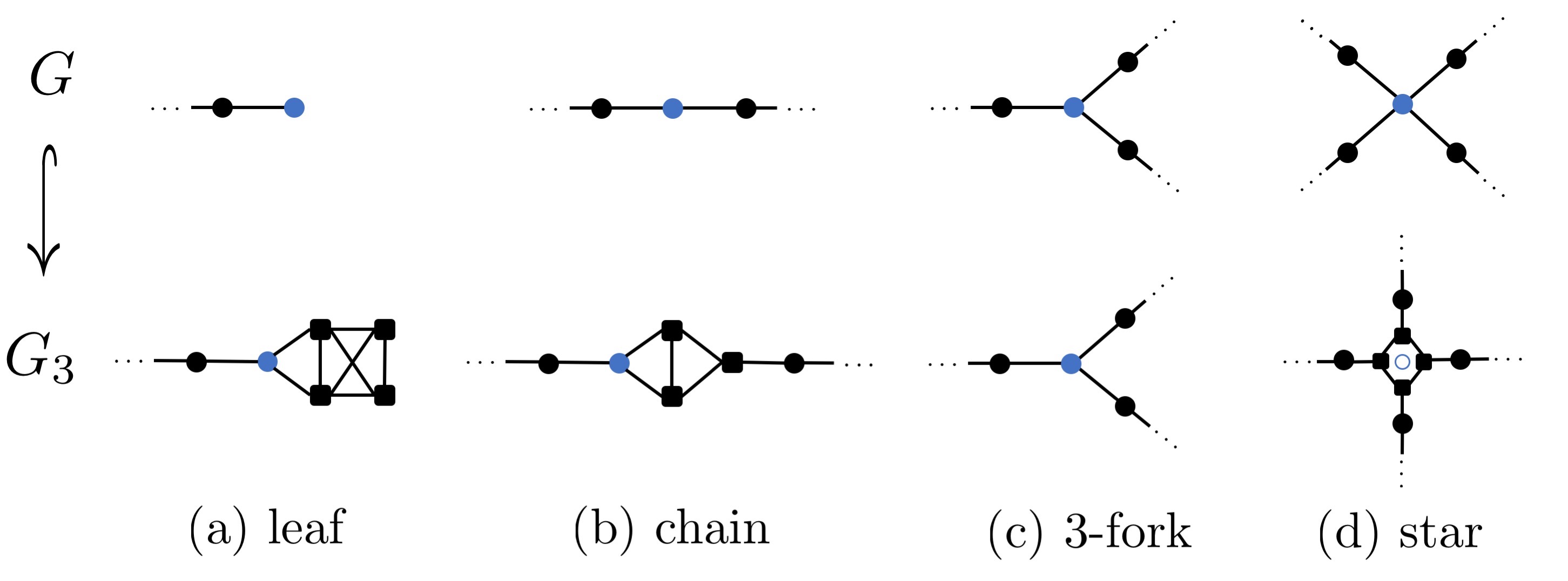
Figure 1: Regularization $G\hookrightarrow G_{3}$ following [4]. A vertex $v\in V$ is called leaf, if it has degree 1, chain if it has degree 2, 3-fork, if it has degree 3 and star otherwise. The transformation maps each vertex and the edges connecting to its direct neighbors onto the respective three-regular structure as predicted by the vertex’ degree. Circles represent original vertices, squares auxiliary vertices that have been added to enforce uniform node degrees.

Relational data as typically encountered in data science applications is very heterogeneous, making it difficult to draw a conclusion on the global geometry from local analysis. Our first step is therefore the regularization of the graph’s connectivity structure that will allow for a more efficient comparison of local neighborhood growth rates and, in turn, the local geometry. We will use throughout the paper the following (conventional) notation: When analyzing the neighborhood of a vertex $v\in V$, we say that $v$ is the root or center of the neighborhood. Neighborhood directionality is always assumed from the root outwards, the start of an outward facing edge is called parent, the end child. The root has no parent.

We utilize a quasi-isometric embedding [4] that allows for embedding any (connected) graph into a three-regular graph, i.e. a graph with uniform node degrees (${\rm deg}(v)=3$ for all $v\in V$). The regularization algorithm is shown schematically in Fig. 1, for more details see Appendix A. One can show the following bound on the distortion induced by this transformation:

Theorem 3.1 ( [4]).

$G\hookrightarrow^{\phi}G_{3}$ is a $(\epsilon+1,\epsilon)$-quasi-isometric embedding, i.e. $c_{M}=O(1+\epsilon)$ and $c_{A}=O(\epsilon)$.

3.2 Estimating local neighborhood growth rates

In order to decide the geometry of a suitable embedding space, we want to analyze neighborhood growth rates. Consider first a continuous, metric space ($\mathcal{X},d_{\mathcal{X}}$). The $\delta$-neighborhood of a point $x\in\mathcal{X}$ is defined as the set of points within a distance $\delta$, i.e.

$$\mathcal{B}_{\delta}(x)=\{y\in\mathcal{X}:\;d_{\mathcal{X}}(x,y)\leq\delta\}\;.$$ (1)

In Euclidean space, the volume of $\mathcal{B}_{\delta}(x)$ is growing at a polynomial rate in $\delta$. However, in hyperbolic space, the volume growth is exponential. Therefore, the local volume growth of neighborhoods serves as a proxy for the space’ global geometry.

In discrete space, instead of analyzing volume growth, we characterize the local growth of neighborhoods. We denote the $r$-neighborhood of a vertex $v\in V(G)$ as

$$\mathcal{N}_{r}(v)=\{u\in V(G):d_{G}(u,v)\leq r\}\;.$$ (2)

We say that $\mathcal{N}_{r}(v)$ is exponentially expanding, if it grows exponentially in $r$ and linearly expanding, if it grows at least linearly in $r$. Otherwise, we call $\mathcal{N}_{r}(v)$ sublinearly expanding. Thanks to the regularized structure of our graphs, we can quantify precisely the corresponding neighborhood growth laws:

1. exponentially expanding:
   $\gamma_{EE}(v,R)=|v|+\sum_{r=1}^{R}3\cdot 2^{r-1}$;

2. linearly expanding:
   $\gamma_{LE}(v,R)=|v|+\sum_{r=1}^{R}3r$.

Here, $|v|$ denotes the size of the root structure, i.e., $|v|=1$, if ${\rm deg}(v)\leq 3$ and $|v|={\rm deg}(v)$ otherwise, due to the transformation of star-nodes into three-regular rings (see Fig. 1 and Appendix A). Then we say that the $R$-neighborhood of a vertex $u\in V(G)$ is exponentially expanding, if $|\mathcal{N}_{R}(u)|\geq\gamma_{EE}(R)$, linearly expanding, if $|\mathcal{N}_{R}(u)|\geq\gamma_{LE}(R)$ and sublinearly expanding otherwise. For canonical graphs, we get the following neighborhood growth rates (a proof can be found in Appendix B):

Theorem 3.2 (Neighborhood growth in canonical graphs).

For $1\leq R\ll N$, every $R$-neighborhood in (i) a $b$-regular tree is exponentially expanding, (ii) an ($\sqrt{N}\times\sqrt{N}$)-lattice is linearly expanding and (iii) an $N$-cycle is sublinearly expanding.

Utilizing the link between neighborhood growth and global geometry that we discussed above, we introduce the following decision rule for the geometric prior of the embedding space (${\rm sign}(\kappa)$):

• If $\mathcal{N}_{R}(v)$ is exponentially expanding $\forall v\in V$ and $1\leq R\ll N$, assume ${\rm sign}(\kappa)<0$, i.e., embed into $\mathbb{H}^{d}$;

• If $\mathcal{N}_{R}(v)$ is lineraly expanding $\forall v\in V$ and $1\leq R\ll N$, assume ${\rm sign}(\kappa)=0$, i.e., embed into $\mathbb{R}^{d}$;

• If $\mathcal{N}_{R}(v)$ is sublinearly expanding $\forall v\in V$ and $1\leq R\ll N$, assume ${\rm sign}(\kappa)>0$, i.e., embed into $\mathbb{S}^{d}$.

Note that these result match known embeddability results for canonical graphs (see Table 2). In the following section we introduce a statistic that allows for applying this decision rule to heterogeneous relational data also.

3.3 3-Regular Score

The heterogeneity commonly encountered in relational data makes it impossible to generalize global growth rates from a local analysis as in Thm. 3.2. We will typically find a mixture of local growth rates, that is not covered by the decision rule above. Instead, we focus on determining the globally dominating geometry: We analyze growth rates locally and then compute an average across the graph, weighted by the size of the respective $R$-neighborhood. The resulting statistic, to which we refer as the 3-regular score, can be computed as follows:

$$A =\sum_{v\in V}\sigma(v)|\mathcal{N}_{R}(v)|\;;$$

$$\sigma(v) =\begin{cases}1,&\mathcal{N}_{R}(v)\;{\rm sublinearly\;expanding}\\ -1,&\mathcal{N}_{R}(v)\;{\rm exponentially\;expanding}\\ 0,&{\rm otherwise}\;.\end{cases}$$

To determine the geometric priors, we apply the following decision rule:

• if $A>0$, assume ${\rm sign}(\kappa)>0$, i.e., embed into $\mathbb{S}^{d}$;

• if $A<0$, assume ${\rm sign}(\kappa)<0$, i.e., embed into $\mathbb{H}^{d}$;

• and if $A\approx 0$, assume ${\rm sign}(\kappa)=0$, i.e., embed into $\mathbb{R}^{d}$.

For weighted networks, we perform the same regularization and computation of the 3-regular score, but replace in the growth rate estimations $3$ with the weighted node degree of the center. When determining $|\mathcal{N}_{R}(v)|$, i.e., the set of all neighbors up to distance $R$ from $v$, the metric is the weighted path distance $\tilde{d}_{G}$. Consequently, we count all neighbors $v^{\prime}$ with $\tilde{d}_{G}(v,v^{\prime})\leq R$.

The decision rule is motivated by locally aggregating neighborhood growth information. Hereby $\sigma$ encodes whether the neighborhood growth is locally exponential (indicating hyperbolic space, i.e., ${\rm sign}(\kappa)=-1$ and $\sigma=-1$), linear (indicating Euclidean space, i.e., $\kappa=0$ and $\sigma=0$) or sublinear (indicating spherical space, i.e., ${\rm sign}(\kappa)=1$ and $\sigma=-1$). Due to the heterogeneity of the graphs, we weigh the $\sigma$s by the size of the neighborhood ($|\mathcal{N}_{R}(v)|$) to give large neighborhoods a larger influence on the overall score. This is motivated by the fact that the ”amount” of distortion incurred is proportional to the largest subgraph of another space’s canonical motif: For instance, when embedding a graph into hyperbolic space, distortion is proportional to the size of the largest cycle by a Steiner node construction (see, e.g., [30]). The resulting 3-regular score $A$ after reweighing will then depend on the size of the graph, in particular on the number of edges in the regularized graph $G_{3}$. Therefore, we normalize by dividing by the the number of edges in $G_{3}$, i.e., we compare $A/\#E(G_{3})$ across data sets. The dependency of $A$ on $R$ is explicitly given through the weights $|\mathcal{N}_{R}(v)|$; $R$ is upper-bounded by the diameter of the graph.

3.4 Comparison with other discrete curvatures

The 3-regular score is conceptually related to discrete notions of curvature, such as Gromov’s $\delta$-hyperbolicity [15] or discrete Ricci curvature [14, 25]. While Gromov’s $\delta$ captures by construction the hyperbolicity of a graph, discrete Ricci curvature is not restricted to negative values. In this section, we analyze the relationship between the 3-regular score and discrete Ricci curvature and compare the suitability of both concepts to measure embeddability.

In the following, we will think of data sets as graphs, where nodes represent the data points and edges the pairwise similarities between them. For simplicity, we only consider unweighted graphs. We consider both Ollivier-Ricci curvature (${\rm Ric_{O}}$) [25] and Forman-Ricci curvature (${\rm Ric_{F}}$) [14, 33] that have previously been analyzed in the context of large-scale data and complex networks. Although both curvatures are classically defined edge-based, we will use node-based expressions. Those can be derived by defining the Ricci curvature at a node as the aggregate curvature of its incoming and outgoing edges (see Appendix C for more details). For ${\rm Ric_{O}}$, consider

$${\rm Ric_{O}}(u,v)=1-W_{1}(m_{u},m_{v})\;,$$

where $W_{1}(m_{u},m_{v})$ is the Wasserstein-1 distance that measures the cost of transporting mass from $u$ to $v$. $m_{u}=\frac{1}{{\rm deg}(u)}$ denotes the uniform measure on the neighborhood of $v$. The corresponding node-based notion is given by

$${\rm Ric_{O}}(v)=\frac{1}{{\rm deg}}\sum_{(u,v)}{\rm Ric_{O}}(u,v)\;.$$

${\rm Ric_{F}}$ of an edge $(u,v)$ is defined as

$${\rm Ric_{F}}(u,v)=4-{\rm deg}(u)-{\rm deg}(v)\;,$$

the corresponding node-based expression as

$${\rm Ric_{F}}(v)=\frac{1}{{\rm deg}}\sum_{(u,v)}{\rm Ric_{F}}(u,v)\;.$$

The aggregation of local growth rates in the 3-regular score resembles the Ricci curvature’s property of ”locally averaging” sectional curvature. Note that both Ricci curvatures encode only structural information of the first and second neighbors, whereas the 3-regular score measures structural information from neighbors up to distance $R$. Both ${\rm Ric_{F}}$ and the 3-regular score are very scalable due to their simple combinatorial notion. ${\rm Ric_{O}}$ has limited scalability on large-scale data, since the computation of Wasserstein distances requires solving a linear program for every edge.

To evaluate whether Ricci curvature can select a suitable embedding space, we consider again canonical graphs. Due to their regular structure, the global average curvature is equal to the local curvature at any node in the graph. We derive the following results:

Theorem 3.3.

At any node $v$, we have

1. ${\rm Ric_{O}}(v)<0$ and ${\rm Ric_{F}}(v)<0$ in a $b$-regular tree,

2. ${\rm Ric_{O}}\leq 0$ and ${\rm Ric_{F}}(v)<0$ in an ($\sqrt{N}\times\sqrt{N}$)-lattice, and

3. ${\rm Ric_{O}}=0$ and ${\rm Ric_{F}}=0$ in an $N$-cycle.

The proof follows from combinatorial arguments and (for ${\rm Ric_{O}}$) curvature inequalities [19]; it can be found in Appendix C. The theorem shows that Ricci curvature, similar to Gromov’s $\delta$, correctly detects hyperbolicity, but cannot characterize structures with non-negative curvature. We conclude, that Ricci curvature is not suitable for model selection and that the 3-regular score has broader applicability.

4 Experiments

We have shown above, that in the case of canonical graphs, our approach’s prediction matches known embeddability results. In this section, we want to experimentally validate that the 3-regular score determines suitable embedding spaces for complex, heterogeneous data. In the following, we report “normalized” 3-regular scores, meaning that we divide by the number of edges in the regularized graph multiplied by the mean edge weight. This adjusts for differences in the average neighborhood size and therefore allows for a comparison across data sets of varying sizes.

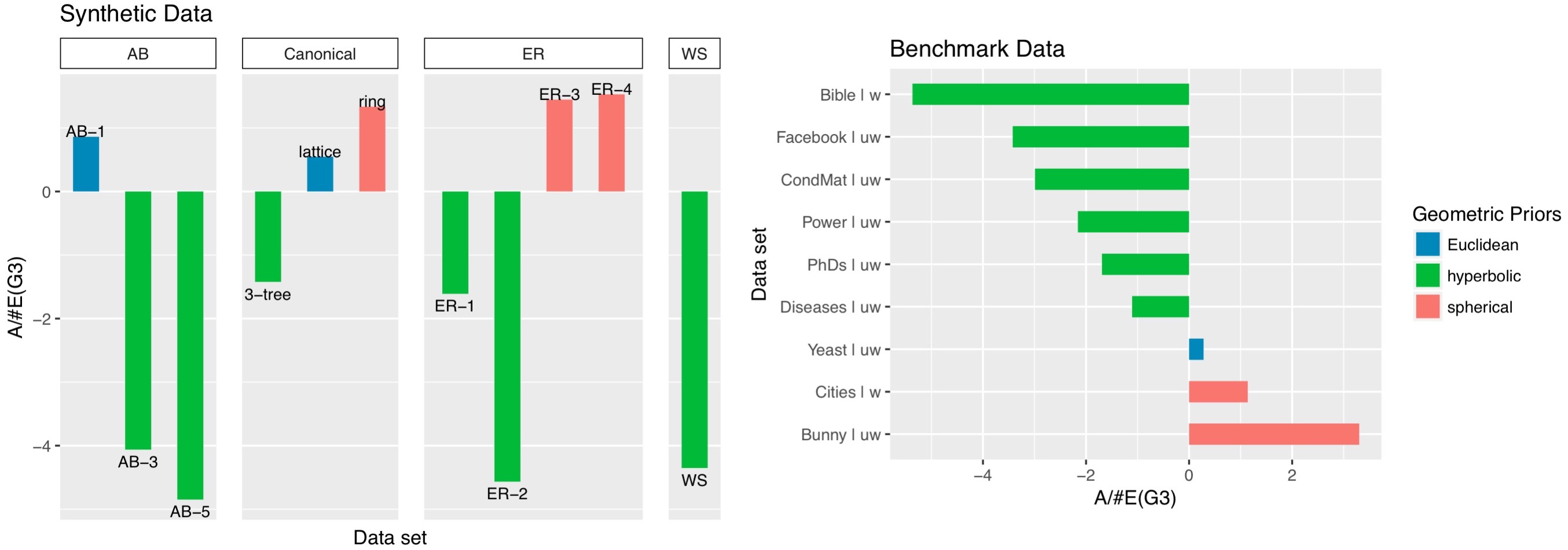
Figure 2: 3-regular scores for synthetic graphs and relational benchmark data (w: weighted, uw: unweighted).

Data sets

We test our method on both synthetic graphs with known embeddability properties and benchmark data sets. For the former, we create data sets of similar size ($N:=|V|\approx 1,000$) to allow for direct comparison. First we generate an $N$-Cycle, an ($\sqrt{N}\times\sqrt{N}$)-lattice and a ternary tree ($b=3$) with $N$ nodes. We further sample from three classic network models: The random graph model (ER) [13], the small world model (WS) [31] and the preferential-attachment model (AB) [3] with different choices of hyperparameters. We sample ten networks each and report the average 3-regular score to account for structural sampling variances. Next, we analyze some classic benchmark graphs (both weighted and unweighted) which were downloaded from the Colorado Networks Index [11]. The Bunny data was downloaded from the Stanford 3D Scanning Repository [28]. Finally, for validating our approach against recently published embeddability results, we analyze data sets used in [16, 23], downloaded from the given original sources. We evaluate geographic distances between North American cities (Cities [8]), PhD student-adviser relationships (PhD, [12]) and a citation networks (CondMat, [21]). Cities contains similarity data from which we created a nearest-neighbor graph, maintaining edges to the top $5\%$ neighboring cities.

Results

3-regular scores for all data sets are shown in Fig. 2. For canonical graphs, the 3-regular score matches both the theoretical results of our growth rate analysis (Thm. 3.2) and embeddability results in the literature (Tab. 2). It is well known that ER undergoes phase transitions as the edge threshold increases. [10] show that ER is not hyperbolic in the low edge threshold regime, but that hyperbolicity emerges with the giant component due to its locally tree-like structure. We analyze ER shortly above (ER-3) and below (ER-4) the giant threshold ($p=\frac{1}{N}$) as well as shortly above (ER-2) and below (ER-1) the connectivity threshold ($p=\frac{\log N}{N}$). Consistent with the theoretical result of [10], we observe hyperbolicity, if there is a large giant component (ER-1) or if the graph is connected (ER-2). For AB with linear attachment ($m=1$), the 3-regular score predicts a Euclidean embedding space to be most suitable, as opposed to hyperbolic embeddings for the case of superlinear attachment ($m>1$). This is again consistent with theoretical results on phase transitions in the AB model. The presence of detectable network communities, as found for instance in social networks, has been repeatedly linked to a locally tree-like structure [2, 20]. In agreement with this, the 3-regular score predicts good hyperbolic embeddability for both WS (a classic model for studying community structure) and the social network data sets Facebook and PhD. The wordnet Bible was found to embed best into hyperbolic space, in-line with the tree-likeness of such intrinsically hierarchical data. [26] observed “less hyperbolicity” in biological networks, which matches our results for Diseases and Yeast. Finally, Bunny, a classic benchmark for spherical embeddings, is found to embed best into spherical space.

Validation and comparison with related methods

To validate our results, we compare our predicted geometric priors against recently published embeddability results by [16, 23]. Table 3 shows that the 3-regular score predicts the space with the smallest distortion for all benchmark data sets. Here, we follow the authors in reporting distortion using the following statistics: The average distortion ${\rm D_{avg}}$, computed over all pairwise distances, and the structural distortion score ${\rm MAP}$ that measures the preservation of nearest-neighbor structures. Isometric embeddability is characterized by ${\rm D_{avg}}=0$ and ${\rm MAP}=1$. For more details, see Appendix D.

Data set	3-regular score	dist $\mathbb{R}^{10}$	dist $\mathbb{S}^{10}$	dist $\mathbb{H}^{10}$	Method
Cities	1.138 $\rightarrow\mathbb{S}^{d}$	$D_{avg}=0.074$	$\bm{{\rm D_{avg}}=0.060}$	${\rm D_{avg}}=0.093$	Gu et al.
PhD students	-1.691 $\rightarrow\mathbb{H}^{d}$	$D_{avg}=0.054$ ${\rm MAP}=0.869$	$D_{avg}=0.057$ ${\rm MAP}=0.833$	$\bm{{\rm D_{avg}}=0.050}$ $\bm{{\rm MAP}=0.931}$	Gu et al.
Power	-2.158 $\rightarrow\mathbb{H}^{d}$	${\rm D_{avg}}=0.092$ $\bm{{\rm MAP}=0.886}$	${\rm D_{avg}}=0.050$ ${\rm MAP}=0.795$	$\bm{{\rm D_{avg}}=0.039}$ ${\rm MAP}=0.844$	Gu et al.
Facebook	-3.423 $\rightarrow\mathbb{H}^{d}$	${\rm D_{avg}}=0.065$ ${\rm MAP}=0.580$	${\rm D_{avg}}=0.066$ ${\rm MAP}=0.556$	$\bm{{\rm D_{avg}}=0.060}$ $\bm{{\rm MAP}=0.782}$	Gu et al.
CondMat	-2.991 $\rightarrow\mathbb{H}^{d}$	${\rm MAP}=0.356$	-	$\bm{{\rm MAP}=0.799}$	Nickel, Kiela

Table 3: Comparison with recently published benchmark embeddability results [16, 23].

Hyperparameters

The size of the local neighborhoods $\mathcal{N}_{R}(v)$ over which we compute the 3-regular score (determined by the neighborhood radius $R$) is the central hyperparameter in our analysis. Choosing $R$ too small might leave us with too little information to properly evaluate growth rates, whereas a large $R$ limits scalability. First, note that for $R<3$, $\gamma_{EE}=\gamma_{LE}$ in the regularized graph $G_{3}$. However, for $R\geq 3$ we always have $\gamma_{EE}\neq\gamma_{LE}$. Consequentially, we require $R\geq 3$. Next, we investigated experimentally if an analysis with larger neighborhood radii reveals additional geometric information by computing 3-regular scores for three data sets with different predicted geometric priors for $R\in\{3,4,5,10\}$. For the ($\sqrt{N}\times\sqrt{N}$)-lattice, the 3-regular score predicts uniformly ${\rm sign}(\kappa)=0$, i.e. $\mathbb{R}^{d}$ to be the most suitable embedding space. For WS we observe ${\rm sign}(\kappa)=-1$ across all choices of $R$, predicting hyperbolic embeddability. Finally, for Cities we observe ${\rm sign}(\kappa)=1$ across the different neighborhood radii. In consequence, the 3-regular scores reported above are all computed for $R=3$ to maximize scalability.

5 Discussion

In this paper, we introduced a framework for determining a suitable embedding curvature for relational data. Our approach evaluates local neighborhood growth rates based on which we approximate suitable embedding curvatures. We provide theoretical guarantees for canonical graphs and introduce a statistic that efficiently aggregates local growth information, rendering the method applicable to heterogeneous, large-scale graphs (both weighted and unweighted). Moreover, we compare the 3-regular score with commonly used notions of discrete curvature in terms of their ability to measure embeddability. We find that discrete curvature is suitable for detecting hyperbolicity, but not for approximating non-negative sectional curvature. This implies that the 3-regular score is better suited for model space selection.
Contrary to related embeddability methods, our approach is purely combinatorial, circumventing the need to solve costly large-scale optimization problems. Furthermore, the method does not make any a priori assumption on the dimensionality of the embedding space as opposed to related approaches that impose dimensionality constraints or fix the dimension of the target space. Additionally, the locality of the approach confines the analysis to a small subset of the graph at any given time, allowing for a simple parallelization of the method. This increases the algorithm’s scalability significantly.
Our results tie into the more general problem of finding data representations that reflect intrinsic geometric and topological features. This problem is three-fold: It requires us to determine (i) the sign of the curvature, which in turn determines the model space, i.e. whether to embed in hyperbolic ($\mathbb{H}^{d}$), spherical ($\mathbb{S}^{d}$) or Euclidean space ($\mathbb{R}^{d}$). Furthermore, (ii) the value of the curvature, which determines local and global geometric parameters of the embedding space, such as distance and angle relations in geodesic triangles and lastly (iii) the dimension of the embedding space. The present work mostly focuses on (i) as we restrict our analysis to canonical Riemannian manifolds with constant sectional curvature ($\kappa\in\{\pm 1,0\}$). By combining this approach with MDS-style embedding methods [16, 26, 7] we could determine the value of the curvature (problem (ii)) also. Hereby, prior knowledge of the sign of the curvature determines the metric of the target space (with the curvature value as hyperparameter) and therefore a suitable objective function to feed into an MDS-style framework. Such a pre-analysis with combinatorial methods should significantly narrow down the search space of suitable curvature values and therefore reduce the overall computational cost. The investigation of such extensions is left for future work.

Appendix A Regularization

We perform a regularization of our graphs (see section 3) which allows for an efficient characterization of local neighborhood growth rates and in turn, the local geometry. In this appendix, we provide more details on the implementation and the theoretical guarantees of the regularization.

Fig. 1 shows the regularization schematically. For each vertex $v$ in the graph, we enforce a uniform node degree of 3 within its 1-hop neighborhood $\mathcal{N}_{1}(v)$. Hereby auxiliary vertices $a$ are inserted and modified edges reweighed. The regularization algorithm is given in Alg. 1.

Algorithm 1 Regularization

1:Input: $G=\{V(G),E(G)\}$

2:$\epsilon\leftarrow\max_{e\in E}\omega(e)$

3:for $v\in V$ do

4:     $\mathcal{N}(v)\leftarrow\{u\in V:v\sim u\}$ $\triangleright$ Neighborhood of $v$.

5:     if ${\rm deg}(v)==1$ then $\triangleright$ Leaf: $\mathcal{N}(v)=\{u\}$

6:         Create($a^{0},a^{1},a^{2},a^{3}$) $\triangleright$ auxiliary nodes

7:         $\omega(u,v)\leftarrow\omega(u,v)/2$

8:         $\omega(v,a^{0}),\;\omega(v,a^{1})\leftarrow\epsilon/4$

9:         $\omega(a^{i},a^{i+k})\leftarrow\epsilon/4$ for $i=0,1$; $k=1,2$

10:     else if ${\rm deg}(v)==2$ then $\triangleright$ Chain: $\mathcal{N}(v)=\{u_{1},u_{2}\}$

11:         Create($a^{0},a^{1},a^{2}$) $\triangleright$ auxiliary nodes

12:         $\omega(u_{1},v)\leftarrow\omega(u_{1},v)/2$

13:         $\omega(v,a^{i})\leftarrow\omega(u_{2},v)/2$ for $i=0,1$

14:         $\omega(u_{2},a^{2})\leftarrow\omega(u_{2},v)/2$

15:         $\omega(a^{0},a^{1}),\;\omega(a^{0},a^{2}),\;\omega(a^{1},a^{2})\leftarrow\epsilon/4$

16:     else if ${\rm deg}(v)==3$ then $\triangleright$ 3-regular: $\mathcal{N}(v)=\{u_{1},u_{2},u_{3}\}$

17:         Continue

18:     else$\triangleright$ Star: $\mathcal{N}(v)=\{u_{i}\}_{i=1}^{{\rm deg}(v)}$

19:         Create($a^{1},\dots,a^{{\rm deg}(v)}$) $\triangleright$ auxiliary nodes

20:         for $i=1,\dots,{\rm deg}(v)$ do

21:              $\omega(a^{i},u^{i})\leftarrow\omega(u_{i},v)/2$

22:              $\omega(a^{i},a^{i+1})\leftarrow\epsilon/4$

23:         end for

24:     end if

25:end for

The regularization allows for a quasi-isometric embedding of any graph into a 3-regular graph. We provide the theoretical reasoning below:

Theorem A.1 (Bermudo et al. [4]).

$G\hookrightarrow^{\phi}G_{3}$ is a $(\epsilon+1,\epsilon)$-quasi-isometric embedding, i.e.

$$d_{G_{3}}(\phi(x),\phi(y))\leq(\epsilon+1)d_{G}(x,y)+\epsilon\;.$$ (3)

From this we can derive the following additive distortion:

$$|d_{G_{3}}-d_{G}|\leq|(\epsilon+1)d_{G}+\epsilon-d_{G}|=|\epsilon(\underbrace{d_{G}}_{\leq{\rm diam}(G)}+1)|\leq O(\epsilon)\;,$$

For the multiplicative distortion we have

$$d_{G}\leq d_{G_{3}}\leq(1+\epsilon)d_{G}+\epsilon\\ \Rightarrow\frac{1}{1+\epsilon}d_{G}\leq d_{G_{3}}\leq(\underbrace{d_{G}}_{\leq{\rm diam}(G)}+1)(1+\epsilon)\leq O(1+\epsilon)\;.$$

This gives $c_{A}=O(\epsilon)$ and $c_{M}=O(1+\epsilon)$ as given in the main text.

Appendix B Neighborhood growth rates in canonical graphs

We restate the result from the main text:

Theorem B.1 (Neighborhood growth of canonical graphs).

For $3\leq R\ll N$, every $R$-neighborhood in

1. a $b$-regular tree is exponentially expanding;

2. an ($\sqrt{N}\times\sqrt{N}$)-lattice is linearly expanding;

3. an $N$-cycle is sublinearly expanding.

Proof.

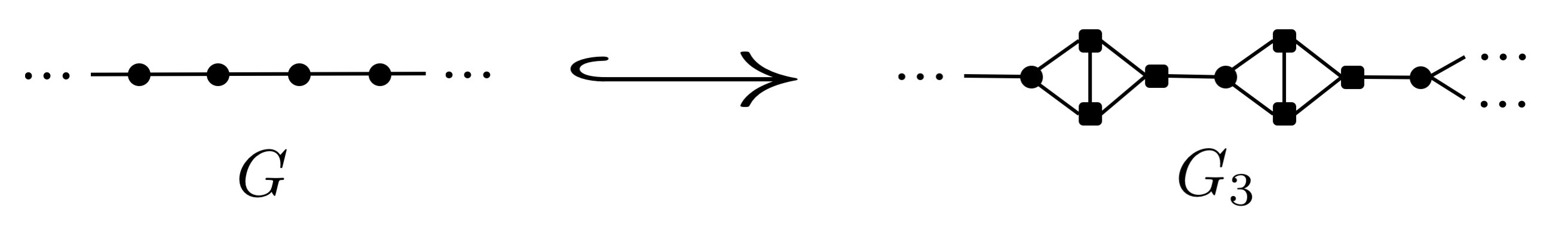
Figure 3: Regularization of $N$-cycle.

The regularization introduces edge weights (see Alg. 1), however, due to the periodic structure of the canonical graphs, those weights are uniform (for lattices and trees) or up to an additive error of $\frac{\epsilon}{4}$ uniform (for cycles). Therefore, we can renormalize the edge weights and analyze the regularized graphs as unweighted graphs. For cycles, the residual additive error does not affect the neighbor count and can therefore be neglected.

Consider first (c) an $N$-cycle. Due to the periodic structure of the chains in the regularized graph (see Fig. 3), there are always either two or three vertices at a distance $r$ from the root, in particular, we have

$$|\mathcal{N}_{R}(v)| =1+\sum_{r=1}^{R}\alpha(r)\;,$$

$$\alpha(r) =\begin{cases}2,&{\rm mod(r,3)=0}\\ 3,&{\rm else}\end{cases}\;.$$

It is clear that $\sum_{r=1}^{R}\alpha(r)<3R$, i.e. the growth is sublinear.

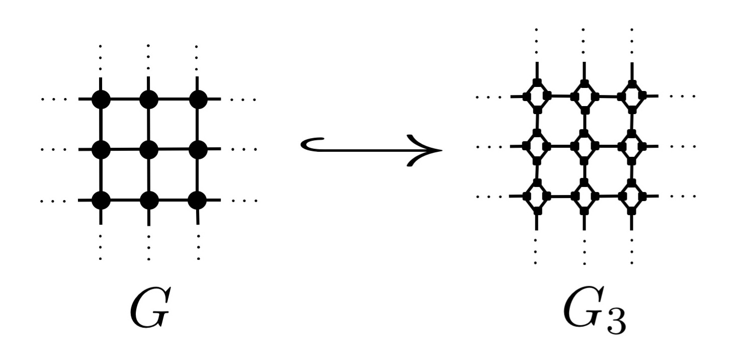
Figure 4: Regularization of ($\sqrt{N}\times\sqrt{N}$)-cycle.

Next, consider (b) a ($\sqrt{N}\times\sqrt{N}$)-lattice. From the periodicity of the regularized graph (see Fig. 4), we see that the number of nodes at distance $r$ from the root grows linearly in $r$. In particular, we have

$$|\mathcal{N}_{R}(v)| =|v|+\sum_{r=1}^{R}{\rm deg}(v)\alpha(r)\;,$$

$$\alpha(r) =\begin{cases}r-1,&{\rm mod(r,3)=1}\\ r,&{\rm else}\end{cases}\;.$$

Since ${\rm deg}(v)=4$, we have ${\rm deg}(v)\alpha(r)\geq 3r$, i.e. the lattice expands linearly.

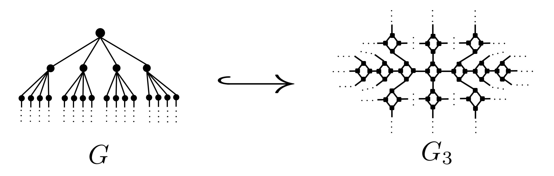
Figure 5: Regularization of $b$-ary tree (here $b=4$).

Finally, consider (a) a $b$-ary tree. We first consider the case $b=3$, i.e., a ternary tree. Note that this structure is invariant under our regularization. Since every node has exactly two children, we get the following growth rate:

$$|\mathcal{N}_{R}(v)|=1+\sum_{r=1}^{R}3\cdot 2^{r-1}=\gamma_{EE}\;,$$

i.e., the ternary tree expands exponentially. Now consider general $b$-ary trees with $b>3$. The building blocks of the periodic structure unfolding are $b$-rings (see Fig. 5). On each level, the nodes have either two children or two nodes have a combined three children, if the $b$-rings close. This results in the following growth rate:

$$|\mathcal{N}_{R}(v)| =|v|+\sum_{r=1}^{R}b\cdot\alpha(r)\;,$$

$$\alpha(r) =\begin{cases}\frac{3}{2}\cdot 2^{r-1},&{\rm mod(\lceil\frac{r}{2}\rceil,b)=b-1}\\ 2^{r},&{\rm else}\end{cases}\;.$$

Since $3<b$ and $2^{r-1}<\alpha(r)$, all $b$-regular trees expand exponentially. ∎

Appendix C Comparison with other discrete curvatures

We restate the result from the main text (Thm. 3.3):

Theorem C.1.

At any node $v$, we have

1. ${\rm Ric_{O}}(v)<0$ and ${\rm Ric_{F}}(v)<0$ in a $b$-regular tree,

2. ${\rm Ric_{O}}\leq 0$ and ${\rm Ric_{F}}(v)<0$ in an ($\sqrt{N}\times\sqrt{N}$)-lattice, and

3. ${\rm Ric_{O}}=0$ and ${\rm Ric_{F}}=0$ in an $N$-cycle.

Before proving the theorem, recall the node-based curvature notions for $v\in V(G)$:

$${\rm Ric_{O}}(v) =\frac{1}{{\rm deg}(v)}\sum_{(u,v)}{\rm Ric_{O}}(u,v)=\frac{1}{{\rm deg}(v)}\sum_{(u,v)}1-W_{1}(m_{u},m_{v})$$

$${\rm Ric_{F}}(v) =\frac{1}{{\rm deg}(v)}\sum_{(u,v)}{\rm Ric_{F}}(u,v)=4-{\rm deg}(v)-\sum_{(u,v)}\frac{{\rm deg(u)}}{{\rm deg}(v)}\;.$$

Furthermore recall the following curvature inequalities for ${\rm Ric_{O}}$:

Lemma C.2.

[19] ${\rm Ric_{O}}$ fulfills the following inequalities:

1. If $(u,v)$ is an edge in a tree, then ${\rm Ric_{O}}(u,v)\leq 0$.

2. For any edge $u,v$ in a graph, we have

   $$-2\left(1-\frac{1}{{\rm deg}(u)}-\frac{1}{{\rm deg}(v)}\right)_{+}\leq{\rm Ric_{O}}(u,v)\leq\frac{\#(u,v)}{\max\{{\rm deg}(u),{\rm deg}(v)\}}\;,$$

   where $\#(u,v)$ denotes the number of common neighbors (or joint triangles) of $u$ and $v$.

Proof.

(Thm. 3.3) Consider first (3) an $N$-cycle. By Lem. C.2(2) we have for any $(u,v)$ on the right hand side ${\rm Ric_{O}}(u,v)\leq 0$, since a cycle has no triangles. Furthermore, the left hand side gives ${\rm Ric_{O}}(u,v)\geq 0$, since ${\rm deg}(v)={\rm deg}(u)=2$. This implies ${\rm Ric_{O}}(v)=0$. We also have

$${\rm Ric_{F}}(v)=4-{\rm deg}(v)-\left(\frac{{\rm deg}(u_{1})}{2}+\frac{{\rm deg}(u_{2})}{2}\right)=0\;,$$

since ${\rm deg}(v)={\rm deg}(u_{i})=2$.

Next, consider (1) a $b$-ary tree. By Lem. C.2(1), we have $Ric_{O}(u,v)\leq 0$ and therefore $Ric_{O}(v)\leq 0$. Moreover, we have

$${\rm Ric}_{F}(v)=4-(b+1)-\frac{(b+1)(b+1)}{b+1}\leq 0\;,$$

since by construction $b\geq 2$.

Finally, consider (2) an ($\sqrt{N}\times\sqrt{N}$)-lattice. Since the lattice has no triangles, Lem. C.2(2) gives ${\rm Ric_{O}}(u,v)\leq 0$ for any edge $(u,v)$ and therefore ${\rm Ric_{O}}(v)\leq 0$. In addition,

$${\rm Ric}_{F}(v)=4-{\rm deg}(v)-\left(\frac{{\rm deg}(u_{1})}{4}+\frac{{\rm deg}(u_{2})}{4}+\frac{{\rm deg}(u_{3})}{4}+\frac{{\rm deg}(u_{4})}{4}\right)\leq 0\;,$$

since ${\rm deg}(v)={\rm deg}(u_{i})=4$ for all $i$. ∎

Appendix D Embeddability measures

We evaluate the quality of embeddings using two computational distortion measures, following the workflow in  [16, 23]. First, we report the average distortion

$$D_{avg}=\sum_{1\leq i\leq j\leq n}\left|\left(\frac{d_{\mathcal{M}}(x_{i},x_{j})}{d_{G}(x_{i},x_{j})}\right)^{2}-1\right|\;.$$ (4)

Secondly, we report ${\rm MAP}$ scores that measure the preservation of nearest-neighbor structures:

$${\rm MAP}=\frac{1}{|V|}\sum_{u\in V}\frac{1}{{\rm deg}(u)}\sum_{i=1}^{|\mathcal{N}_{1}(u)|}\frac{|\mathcal{N}_{1}(u)\cap R_{u,i}|}{|R_{u,i}|}\;.$$ (5)

Here, $R_{u,i}$ denotes the smallest set of nearest neighbors required to retrieve the $i^{th}$ neighbor of $u$ in the embedding space $M$. One can show that for isometric embeddings, ${\rm D_{avg}}=0$ and ${\rm MAP}=1$.

References

- [1] Ittai Abraham, Yair Bartal, and Ofer Neiman. Embedding metric spaces in their intrinsic dimension. In Proceedings of the Nineteenth Annual ACM-SIAM Symposium on Discrete Algorithms, SODA ’08, pages 363–372, Philadelphia, PA, USA, 2008. Society for Industrial and Applied Mathematics.
- [2] A. B. Adcock, B. D. Sullivan, and M. W. Mahoney. Tree-like structure in large social and information networks. In 2013 IEEE 13th International Conference on Data Mining, pages 1–10, Dec 2013.
- [3] A. L. Barabási and R. Albert. Emergence of scaling in random networks. In Science, volume 286(5439):509–512, 1999.
- [4] Sergio Bermudo, Jose M. Rodriguez, Jose M. Sigarreta, and Jean-Marie Vilaire. Gromov hyperbolic graphs. Discrete Mathematics, 313(15):1575 – 1585, 2013.
- [5] J. Bourgain. On Lipschitz embedding of finite metric spaces in Hilbert space. Israel Journal of Mathematics, 52(1):46–52, Mar 1985.
- [6] Martin R. Bridson and André Haefliger. Metric Spaces of Non-Positive Curvature, volume 319 of Grundlehren der mathematischen Wissenschaften. Springer Berlin Heidelberg, Berlin, Heidelberg, 1999.
- [7] Alexander M. Bronstein, Michael M. Bronstein, and Ron Kimmel. Generalized multidimensional scaling: A framework for isometry-invariant partial surface matching. Proceedings of the National Academy of Sciences, 103(5):1168–1172, 2006.
- [8] John Burkardt. CITIES – city distance datasets.
- [9] Benjamin Chamberlain, James Clough, and Marc Deisenroth. Neural embeddings of graphs in hyperbolic space. In arXiv:1705.10359 [stat.ML], 2017.
- [10] Wei Chen, Wenjie Fang, Guangda Hu, and Michael W. Mahoney. On the hyperbolicity of small-world and treelike random graphs. Internet Mathematics, 9(4):434–491, 2013.
- [11] Aaron Clauset, Ellen Tucker, and Matthias Sainz. The Colorado index of complex networks, 2016.
- [12] W. de Nooy, A. Mrvar, and V. Batagelj. Exploratory social network analysis with pajek. Cambridge University Press, 2004.
- [13] P. Erdős and A. Rényi. On random graphs i. In Publicationes Mathematicae, volume 6, page 290–297, 1959.
- [14] Forman. Bochner’s method for cell complexes and combinatorial ricci curvature. Discrete & Computational Geometry, 29(3):323–374, 2003.
- [15] M. Gromov. Hyperbolic groups. In Essays in Group Theory, volume 8. Mathematical Sciences Research Institute Publications. Springer, NY, 1987.
- [16] Albert Gu, Frederic Sala, Beliz Gunel, and Christopher Ré. Learning mixed-curvature representations in product spaces. In International Conference on Learning Representations, 2019.
- [17] Anupam Kumar Gupta. Embedding tree metrics into low dimensional euclidean spaces. In STOC, 1999.
- [18] William Johnson and Joram Lindenstrauss. Extensions of Lipschitz mappings into a Hilbert space. In Conference in modern analysis and probability (New Haven, Conn., 1982), volume 26 of Contemporary Mathematics, pages 189–206. American Mathematical Society, 1984.
- [19] Jürgen Jost and Shiping Liu. Ollivier’s ricci curvature, local clustering and curvature-dimension inequalities on graphs. Discrete & Computational Geometry, 51(2):300–322, Mar 2014.
- [20] Dmitri Krioukov, Fragkiskos Papadopoulos, Maksim Kitsak, Amin Vahdat, and Marián Boguñá. Hyperbolic geometry of complex networks. Phys. Rev. E, 82:036106, Sep 2010.
- [21] Jure Leskovec and Andrej Krevl. SNAP Datasets: Stanford large network dataset collection. http://snap.stanford.edu/data, June 2014.
- [22] Pierre-André G Maugis, Sofia C Olhede, and Patrick J Wolfe. Topology reveals universal features for network comparison. arXiv:1705.05677, 2017.
- [23] Maximillian Nickel and Douwe Kiela. Poincaré embeddings for learning hierarchical representations. In Advances in Neural Information Processing Systems 30, pages 6338–6347. 2017.
- [24] Maximillian Nickel and Douwe Kiela. Learning continuous hierarchies in the Lorentz model of hyperbolic geometry. In International Conference on Machine Learning. 2018.
- [25] Yann Ollivier. A survey of Ricci curvature for metric spaces and Markov chains. In Probabilistic Approach to Geometry, pages 343–381. Mathematical Society of Japan, 2010.
- [26] Frederic Sala, Chris De Sa, Albert Gu, and Christopher Re. Representation tradeoffs for hyperbolic embeddings. In Proceedings of the 35th International Conference on Machine Learning, volume 80, pages 4460–4469, 2018.
- [27] Rik Sarkar. Low distortion Delaunay embedding of trees in hyperbolic plane. In Graph Drawing, pages 355–366, Berlin, Heidelberg, 2012. Springer Berlin Heidelberg.
- [28] Stanford Computer Graphics Laboratory. The Stanford 3D Scanning Repository, 2014.
- [29] Alexandru Tifrea, Gary Bécigneul, and Octavian-Eugen Ganea. Poincar’e glove: Hyperbolic word embeddings. ICRL, 2019.
- [30] Kevin Verbeek and Subhash Suri. Metric embedding, hyperbolic space, and social networks. Computational Geometry, 59:1 – 12, 2016.
- [31] D. J. Watts and S. H. Strogatz. Collective dynamics of ’small-world’ networks. In Nature, volume 393(6684):440–442, 1998.
- [32] Melanie Weber and Maximilian Nickel. Curvature and representation learning: Identifying embedding spaces for relational data. In NeurIPS Relational Representation Learning, 2018.
- [33] Melanie Weber, Emil Saucan, and Jürgen Jost. Characterizing complex networks with Forman-Ricci curvature and associated geometric flows. Journal of Complex Networks, 5(4):527–550, 2017.
- [34] Melanie Weber, Emil Saucan, and Jürgen Jost. Coarse geometry of evolving networks. Journal of Complex Networks, 6(5):706–732, 2017.
- [35] R. C. Wilson, E. R. Hancock, E. Pekalska, and R. P. W. Duin. Spherical and Hyperbolic Embeddings of Data. IEEE Transactions on Pattern Analysis and Machine Intelligence, 36(11):2255–2269, 2014.