Fi-GNN: Modeling Feature Interactions via Graph Neural Networks for CTR Prediction

Abstract.

Click-through rate (CTR) prediction is an essential task in web applications such as online advertising and recommender systems, whose features are usually in multi-field form. The key of this task is to model feature interactions among different feature fields. Recently proposed deep learning based models follow a general paradigm: raw sparse input multi-filed features are first mapped into dense field embedding vectors, and then simply concatenated together to feed into deep neural networks (DNN) or other specifically designed networks to learn high-order feature interactions. However, the simple unstructured combination of feature fields will inevitably limit the capability to model sophisticated interactions among different fields in a sufficiently flexible and explicit fashion.

In this work, we propose to represent the multi-field features in a graph structure intuitively, where each node corresponds to a feature field and different fields can interact through edges. The task of modeling feature interactions can be thus converted to modeling node interactions on the corresponding graph. To this end, we design a novel model Feature Interaction Graph Neural Networks (Fi-GNN). Taking advantage of the strong representative power of graphs, our proposed model can not only model sophisticated feature interactions in a flexible and explicit fashion, but also provide good model explanations for CTR prediction. Experimental results on two real-world datasets show its superiority over the state-of-the-arts.

1. Introduction

The goal of click-through rate prediction is to predict the probabilities of users clicking ads or items, which is critical to many web applications such as online advertising and recommender systems. Modeling sophisticated feature interactions plays a central role in the success of CTR prediction. Distinct from continuous features which can be naturally found in images and audios, the features for web applications are mostly in multi-field categorical form. For example, the four-fields categorical features for movies may be: (1) Language = {English, Chinese, Japanese, … }, (2) Genre = {action, fiction, … }, (3) Director = {Ang Lee, Christopher Nolan, … }, and (4) Starring = {Bruce Lee, Leonardo DiCaprio, … } (noted that there are much more feature fields in real applications). These multi-field categorical features are usually converted to sparse one-hot encoding vectors, and then embedded to dense real-value vectors, which can be used to model feature interactions.

Factorization machine (FM) (Rendle, 2010) is a well-known model proposed to learn second-order feature interactions from vector inner products. Field-aware factorization machine (FFM) (Juan et al., 2016) further considers the field information and introduces field-aware embedding. Regrettably, these FM-based models can only model second-order interaction and the linearity modeling limits its representative power. Recently, many deep learning based models have been proposed to learn high-order feature interactions, which follow a general paradigm: simply concatenate the field embedding vectors together and feed them into DNN or other specifically designed models to learn interactions. For example, Factorisation-machine supported Neural Networks (FNN) (Zhang et al., 2016), Neural Factorization Machine (NFM) (He and Chua, 2017), Wide&Deep (Cheng et al., 2016) and DeepFM (Guo et al., 2017) utilize DNN to model interactions. However, these model based on DNN learn high-order feature interactions in a bit-wise, implicit fashion, which lacks good model explanations. Some models try to learn high order interactions explicitly by introducing specifically designed networks. For example, Deep&Cross (Wang et al., 2017) introduces Cross Network (CrossNet) and xDeepFM (Lian et al., 2018) introduces Compressed Interaction Network (CIN). Nevertheless, we argue that they are still not sufficiently effective and explicit, since they still follow the general paradigm of combining feature fields together to model their interactions. The simple unstructured combination will inevitably limit the capability to model sophisticated interactions among different feature fields in a flexible and explicit fashion.

In this work, we take the structure of multi-field features into consideration. Specifically, we represent the multi-field features in a graph structure named feature graph. Intuitively, each node in the graph corresponds to a feature field and different fields can interact through edges. The task of modeling sophisticated interactions among feature fields can be thus converted to modeling node interactions on the feature graph. To this end, we design a novel model Feature interaction Graph Neural Networks (Fi-GNN) based on Graph Neural Networks (GNN), which is able to model sophisticated node (feature) interactions in a flexible and explicit fashion. In Fi-GNN, the nodes will interact by communicating the node states with neighbors and update themselves in a recurrent fashion. At every time step, the model interact with neighbors at one hop deeper. Therefore, the number of interaction steps equals to the order of feature interactions. Moreover, the edge weights reflecting importances of different feature interactions and node weights reflecting importances of each feature field on the final CTR prediction can be learnt by Fi-GNN, which can provide good explanations. Overall, our proposed model can model sophisticated feature interactions in an explicit, flexible fashion and also provide good model explanations.

Our contributions can be summarized in threefold:

• We point out the limitation of the existing works which consider multi-field features as an unstructured combination of feature fields. To this end, we propose to represent the multi-field features in a graph structure for the first time.

• We design a novel model Feature Interaction Graph Neural Networks (Fi-GNN) to model sophisticated interactions among feature fields on the graph-structured features in a more flexible and explicit fashion.

• Extensive experiments on two real-world datasets show that our proposed method can not only outperform the state-of-the-arts but also provide good model explanations.

The rest of this paper is organized as follows. Section 2 summarizes the related work. Section 3 provides an elaborative description of our proposed method. The extensive experiments and detailed analysis are presented in Section 4, followed by the conclusion in Section 5.

2. Related Work

In this section, we briefly review the existing models that model feature interactions for CTR prediction and graph neural networks.

2.1. Feature Interaction in CTR Prediction

Modeling feature interactions is the key to success of CTR prediction and therefore extensively studied in the literature. LR is a linear approach, which can only models the first-order interaction on the linear combination of raw individual features. FM (Rendle, 2010) learns second-order feature interactions from vector inner products. Afterwards, different variants of FM have been proposed. Field-aware factorization machine (FFM) (Juan et al., 2016) considers the field information and introduces field-aware embedding. AFM (Xiao et al., 2017) considers the weight of different second-order feature interactions. However, these approaches can only model second-order interaction which is not sufficient.

With the success of DNN in various fields, researchers start to use it to learn high-order feature interactions due to its deeper structures and nonlinear activation functions. The general paradigm is to concatenate the field embedding vectors together and feed them into DNN to learn the high-order feature interactions. (Liu et al., 2015) utilizes convolutional networks to model feature interactions. Factorisation-machine supported Neural Networks (FNNs) (Zhang et al., 2016) uses the pre-trained factorization machines for field embedding before applying DNN. Product-based Neural Network (PNN) (Qu et al., 2016) models both second-order and high-order interactions by introducing a product layer between field embedding layer and DNN layer. Similarly, Neural Factorization Machine (NFM) (He and Chua, 2017) has a Bi-Interaction Pooling layer between embedding layer and DNN layer to model second-order interactions, but the followed operation is summation instead of concatenation as in PNN. Some works on another line try to model the second-order and high-order interactions jointly via a hybrid architectures. The Wide&Deep (Cheng et al., 2016) and DeepFM (Guo et al., 2017) contain a wide part to model the low-order interaction and a deep part to model the high-order interaction. However, all these approaches leveraging DNN learn the high-order feature interactions in an implicit, bit-wise way and therefore lack good model explainability. Recently, some work try to learn feature interactions in an explicit fashion via specifically designed networks. Deep&Cross (Wang et al., 2017) introduces a CrossNet which takes outer product of features at the bit level. On the contrary, xDeepFM (Lian et al., 2018) introduces a CIN to take outer product at the vector level. Nevertheless, they still don’t solve the most fundamental problem, that is to concatenate the field embedding vectors together. The simple unstructured combination of feature fields will inevitably limit the capability to model sophisticated interactions among different fields in a flexible and explicit fashion. To this end, we proposed to represent the multi-field features in a graph structure, where each node represents a field and different feature fields can interact through the edges. Accordingly, we can model the flexible interactions among different feature fields on the graphs.

2.2. Graph Neural Networks

Graph is a kind of data structure which models a set of objects (nodes) and their relationships (edges). Recently, researches of analyzing graphs with machine learning have been receiving more and more attention because of the great representative power of graphs. Early works usually convert graph-structured data into sequence-structured data to deal with. Inspired by word2vec (Mikolov et al., 2013), the work (Perozzi et al., 2014) proposed an unsupervised DeepWalk algorithm to learn node embedding in graph based on random walks. After that, (Tang et al., 2015) proposed a network embedding algorithm LINE, which preserve the first- and second-order structural information. (Grover and Leskovec, 2016) proposed node2vec which introduces a biased random walk. However, these methods can be computationally expensive and non-optimal for large graphs.

Graph neural networks (GNN) are designed to tackle these problems, which are deep learning based methods that operate on the graph domain. The concept of GNN is first proposed by (Scarselli et al., 2009). Generally, nodes in GNNs interact with neighbors by aggregating information from neighborhoods and updating their hidden states. There have been many variants of GNN with various kinds of aggregators and updaters proposed these days. Here we only present some representative and classical methods. Gated Graph Neural Networks (GGNN) (Li et al., 2015) uses GRU (Cho et al., 2014) as updater. Graph Convolutional Networks (GCN) (Kipf and Welling, 2016) considers the spectral structure of graphs and utilizes the convolutional aggregator. GraphSAGE (Hamilton et al., 2017) considers the spatial information. It introduces three kinds of aggregators: mean aggregator, LSTM aggregator and Pooling aggregator. Graph attention network (GAT) (Veličković et al., 2017) incorporates the attention mechanism into the propagation step. There are some surveys (Wu et al., 2019; Zhou et al., 2018) which provide more elaborative introduction of various kinds of GNN models.

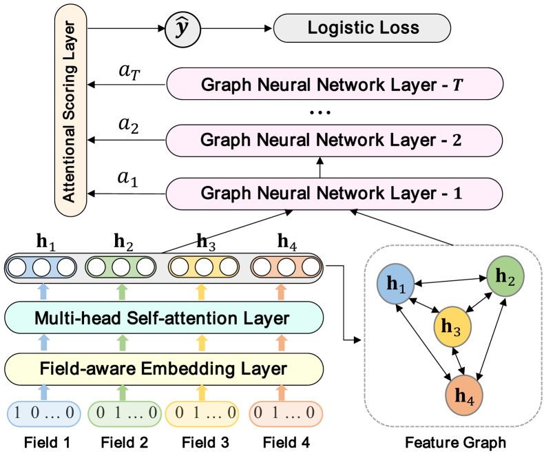
Figure 1. Overview of our proposed method. The input raw multi-field feature vector is first converted to field embedding vectors via an embedding layer and represented as a feature graph, which is then feed into Fi-GNN to model feature interactions. An attention layer is applied on the output of Fi-GNN to predict the click through rate $\hat{y}$. Details of embedding layer and Fi-GNN are illustrated in Figure 2 and Figure 3 respectively.

Due to convincing performance and high interpretability, GNN has been a widely applied graph analysis method. Recently, there are many application of GNN like neural machine translation (Beck et al., 2018), semantic segmentation (Qi et al., 2017), image classification (Marino et al., 2017), situation recognition (Li et al., 2017), recommendation (Wu et al., 2018), script event prediction (Li et al., 2018), fashion analysis (Cui et al., 2019; Li et al., 2019). GNN is suitable for modeling node interactions on graph-structured features intrinsically. In this work, we proposed a model Fi-GNN based on GGNN to model feature interactions on the graph-structured features for CTR prediction.

3. Our Proposed Method

We first formulate the problem and then introduce the overview of our proposed method, followed by the elaborate detail of each component.

3.1. Problem Formulation

Suppose the training dataset consists of $m$-fields categorical features ($m$ is the number of feature fields) and the associated labels $y\in\left\{0,1\right\}$ which indicate user click behaviors. The task of CTR prediction is to predict $\hat{y}$ for the input $m$-fields features, which estimates the probability of a user clicking. The key of the task is to model the sophisticated interactions among different feature fields.

3.2. Overview

Figure 1 is the overview of our proposed method ($m$=4). The input sparse $m$-field feature vector is first mapped into sparse one-hot embedding vectors and then embedded to dense field embedding vectors via the embedding layer and the multi-head self-attention layer. The field embedding vectors are then represented as a feature graph, where each node corresponds to a feature field and different feature fields can interact through edges. The task of modeling interaction can be thus converted to modeling node interactions on the feature graph. Therefore, the feature graph is feed into our proposed Fi-GNN to model node interactions. An attention scoring layer is applied on the output of Fi-GNN to estimate the click-through rate $\hat{y}$. In the following, we will introduce the details of our proposed method.

3.3. Embedding Layer

The multi-field categorical feature $\mathbf{x}$ is usually sparse and of huge dimension. Following previous works (Zhang et al., 2016; Qu et al., 2016; Wang et al., 2017; Guo et al., 2017; Qu et al., 2018), we represent each field as a one-hot encoding vector and then embed it to a dense vector, noted as field embedding vector. Let us consider the example in Section 1, a movie {Language: English, Genre: fiction, Director: Christopher Nolan, Starring: Leonardo DiCaprio } is first transformed into a high-dimensional sparse features via one-hot encoding:

$\underbrace{\left[1,0,...,0\right]}_{\text{Language}},\underbrace{\left[0,1,...,0\right]}_{\text{Genre}},\underbrace{\left[0,1,...,0\right]}_{\text{Director}},\underbrace{\left[0,1,...,0\right]}_{\text{Starring}}$

A field-aware embedding layer is then applied upon the one-hot vectors to embed them to low dimensional, dense real-value field embedding vectors as shown in Figure LABEL:fig:embedding. Likewise, the field embedding vectors of $m$-field feature can be obtained:

$\mathbf{E}=\left[\mathbf{e}_{1},\mathbf{e}_{2},\mathbf{e}_{3},...,\mathbf{e}_{m}\right],$

where $\mathbf{e}_{i}\in\mathbb{R}^{d}$ denotes the embedding vector of field $i$ and $d$ denotes the dimension of field embedding vectors.

3.4. Multi-head Self-attention Layer

Transformer (Vaswani et al., 2017) is prevalent in NLP and has achieved great success in many tasks. At the core of Transformer, the multi-head self-attention mechanism is able to model complicated dependencies between word pairs in multiple semantic subspaces. In the literature of CTR prediction, we take advantage of the multi-head self-attention mechanism to capture the complex dependencies between feature field pairs, i.e, pairwise feature interactions, in different semantic subspaces.

Following (Song et al., 2018), given the feature embeddings $\mathbf{E}$, we obtain the feature representation of features that cover the pairwise interactions of an attention head $i$ via scaled dot-product:

$$\mathbf{H}_{i}=\text{softmax}_{i}(\frac{\mathbf{Q}\mathbf{K}^{T}}{\sqrt{d_{K}}})\mathbf{V},$$

$$\mathbf{Q}=\mathbf{W}_{i}^{(Q)}\mathbf{E},\mathbf{K}=\mathbf{W}_{i}^{(K)}\mathbf{E},\mathbf{V}=\mathbf{W}_{i}^{(V)}\mathbf{E}.$$

The matrices $\mathbf{W}_{i}^{(Q)}\in\mathbb{R}^{d_{i}\times d}$, $\mathbf{W}_{i}^{(K)}\in\mathbb{R}^{d_{i}\times d}$, $\mathbf{W}_{i}^{(V)}\in\mathbb{R}^{d_{i}\times d}$ are three weight parameters for attention head $i$, $d_{i}$ is the dimension size of head $i$, and $\mathbf{H}_{i}\in\mathbb{R}^{m\times d_{i}}$.

Then we combine the learnt feature representations of each head to preserve the pairwise feature interactions in each semantic subspace:

$$\mathbf{H}^{1}=\text{ReLU}(\mathbf{H}_{1}\oplus\mathbf{H}_{2}\oplus\cdots\oplus\mathbf{H}_{h}),$$

where $\oplus$ denotes the concatenation operation and $h$ denotes the number of attention heads. The learnt feature representations $\mathbf{H}^{1}\in\mathbb{R}^{m\times d^{\prime}}$ are used for the initial node states of the graph neural network, where $d^{\prime}=\sum_{i=1}^{h}d_{i}$.

3.5. Feature Graph

Distinguished from the previous works which simply concatenate the field embedding vectors together and feed them into designed models to learn feature interactions, we represent them in a graph structure. In particular, We represent each input multi-field feature as a feature graph $\mathcal{G}=(\mathcal{N},\mathcal{E})$, where each node $n_{i}\in\mathcal{N}$ corresponds to a feature field $i$ and different fields can interact through the edges, so that $\left|\mathcal{N}\right|=m$. Since each two fields ought to interact, it is a weighted fully connected graph while the edge weights reflect importances of different feature interactions. Accordingly, the task of modeling feature interactions can be converted to modeling node interactions on the feature graph.

3.6. Feature Interaction Graph Neural Network

Fi-GNN is designed to model node interactions on the feature graph, which is based on GGNN (Li et al., 2015). It is able to model the interactions in a flexible and explicit fashion.

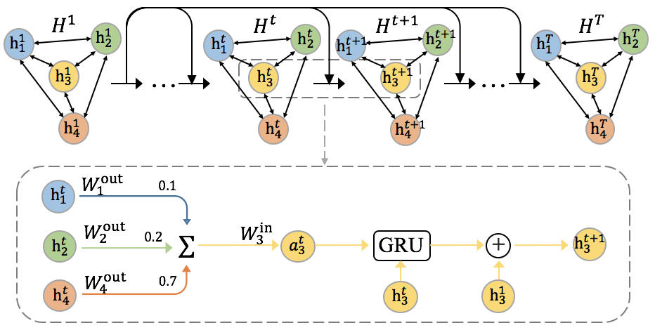
Figure 2. Framework of Fi-GNN. The nodes interact with neighbors and update their states in a recurrent fashion. At each interaction step, each node will first aggregate transformed state information from neighbors and then update its state according to the aggregated information and history via GRU and residual connection.

Preliminaries. In Fi-GNN, each node $n_{i}$ is associated with a hidden state vector $\mathbf{h}_{i}^{t}$ and the state of graph is composed of these node states

$\mathbf{H}^{t}=\left[\mathbf{h}_{1}^{t},\mathbf{h}_{2}^{t},\mathbf{h}_{3}^{t},...,\mathbf{h}_{m}^{t}\right],$

where $t$ denote the interaction step. The learnt feature representations by the multi-head self-attention layer are used for their initial node states $\mathbf{H}^{1}$. As shown in Figure 2, the nodes interact and update their states in a recurrent fashion. At each interaction step, the nodes aggregate the transformed state information with neighbors, and then update their node states according to the aggregated information and history via GRU and residual connection. Next, we will introduce the details of Fi-GNN elaborately.

State Aggregation. At interaction step $t$, each node will aggregate the state information from neighbors. Formally, the aggregated information of node $n_{i}$ is sum of its neighbors’ transformed state information,

(1) $$\mathbf{a}_{i}^{t}=\sum_{n_{j}\rightarrow n_{i}\in\mathcal{E}}\mathbf{A}[n_{j},n_{i}]\mathbf{W}_{p}\mathbf{h}_{j}^{t-1},~{}$$

where $\mathbf{W}_{p}$ is the transformation function. $\mathbf{A}\in\mathbb{R}^{m\times m}$ is the adjacency matrix containing the edge weights. For example, $\mathbf{A}[n_{j},n_{i}]$ is the weight of edge from node $n_{j}$ to $n_{i}$, which can reflect the importance of their interaction. Apparently, the transformation function and adjacency matrix decide on the node interactions. Since the interaction on each edge ought to differ, we aim to achieve edge-wise interaction, which requires a unique weight and transformation function for each edge.

(1) Attentional Edge Weights. The adjacency matrix in the conventional GNN models is usually in the binary form, i.e., only contains 0 and 1. It can only reflect the connected relation of nodes but fails to reflect the importances of their relations. In order to infer the importances of interactions between different nodes, we propose to learn the edge weights via an attention mechanism. In particular, the weight of edge from node $n_{i}$ to node $n_{j}$ is calculated with their initial node states, i.e., the corresponding field embedding vectors. Formally,

(2) $$w(n_{i},n_{j})=\frac{\text{exp}(\text{LeakyRelu}(\mathbf{W}_{w}\left[\mathbf{e}_{i}\left|\right|\mathbf{e}_{j}\right]))}{\sum_{k}\text{exp}(\text{LeakyRelu}(\mathbf{W}_{w}\left[\mathbf{e}_{i}\left|\right|\mathbf{e}_{k}\right]))},$$

where $\mathbf{W}_{w}\in\mathbb{R}^{2d^{\prime}}$ is a weight matrix, $\left|\right|$ is the concatenation operation. The softmax function is utilized to make weights easily comparable across different nodes. Therefore, the adjacency matrix is,

(3) $$\mathbf{A}[n_{i},n_{j}]=\begin{cases}&w(n_{i},n_{j}),\text{ if }i\neq j,\\ &0,\text{ else }.\end{cases}$$

Since the edge weights reflects the importances of different interaction, Fi-GNN can provide good explanations on the relation of different feature fields of input instance, which will be further discussed in Section 4.5.

(2) Edge-wise Transformation. As discussed before, a fixed transformed function on all the edges is unable to model the flexible interactions and a unique transformation for each edge is essential. Nevertheless, our graph is complete graph with a huge number of edges. Simply assigning a unique transformation weight to each edge will consuming too much parameter space and running time. To reduce the time and space complexity and also achieve edge-wise transformation, we assign an output matrix $\mathbf{W}_{out}^{i}$ and an input matrix $\mathbf{W}_{in}^{i}$ to each node $n_{i}$ similar with (Cui et al., 2019). As shown in Figure 2, when node $n_{i}$ sends its state information to node $n_{j}$, the state information will first be transformed by its output matrix $\mathbf{W}_{out}^{i}$ and then transformed by node $n_{j}$’s input matrix $\mathbf{W}_{in}^{j}$ before $n_{j}$ receives it. The transformation function of edge $n_{i}\rightarrow n_{j}$ from node $n_{i}$ to node $n_{j}$ thus could be written as,

(4) $$\mathbf{W}_{p}^{n_{i}\rightarrow n_{j}}=\mathbf{W}_{out}^{i}\mathbf{W}_{in}^{j}.$$

Likewise, the transformation function of edge $n_{j}\rightarrow n_{i}$ from node $n_{j}$ to node $n_{j}$ is

(5) $$\mathbf{W}_{p}^{n_{j}\rightarrow n_{i}}=\mathbf{W}_{out}^{j}\mathbf{W}_{in}^{i}.$$

Accordingly, the Equation 1 could be rewritten as,

(6) $$\mathbf{a}_{i}^{t}=\sum_{n_{j}\rightarrow n_{i}\in\mathcal{E}}\textbf{A}[n_{j},n_{i}]\mathbf{W}_{out}^{j}\mathbf{W}_{in}^{i}\mathbf{h}_{j}^{t-1}+\mathbf{b}_{p}.$$

In this way, the number of parameters is proportional to the number of nodes rather than numerous edges, which greatly reduces the space and time complexity and meanwhile achieves edge-wise interaction.

State Update. After aggregating state information, the nodes will update the state vectors via GRU and residual connections.

(1) State update via GRU. In traditional GGNN, the state vector of node $n_{i}$ is updated via GRU based on the aggregated state information $\mathbf{a}_{i}^{t}$ and its state at last step. Formally,

(7) $$\mathbf{h}_{i}^{t}=GRU(\mathbf{h}_{i}^{t-1},\mathbf{a}_{i}^{t}).$$

It can be formalized in detail as:

(8) $$\mathbf{z}_{i}^{t}=\sigma(\mathbf{W}_{z}\mathbf{a}_{i}^{t}+\mathbf{U}_{z}\mathbf{h}_{i}^{t-1}+\mathbf{b}_{z}),$$

(9) $$\mathbf{r}_{i}^{t}=\sigma(\mathbf{W}_{r}\mathbf{a}_{i}^{t}+\mathbf{U}_{r}\mathbf{h}_{i}^{t-1}+\mathbf{b}_{r}),$$

(10) $$\mathbf{\tilde{h}}_{i}^{t}=tanh(\mathbf{W}_{h}\mathbf{a}_{i}^{t}+\mathbf{U}_{h}(\mathbf{r}_{i}^{t}\odot\mathbf{h}_{i}^{t-1})+\mathbf{b}_{h}),$$

(11) $$\mathbf{h}_{i}^{t}=\mathbf{\tilde{h}}_{i}^{t}\odot\mathbf{z}_{i}^{t}+\mathbf{h}_{i}^{t-1}\odot(1-\mathbf{z}_{i}^{t}),~{}$$

where, $\mathbf{W}_{z}$, $\mathbf{W}_{r}$, $\mathbf{W}_{h}$, $\mathbf{b}_{z}$, $\mathbf{b}_{r}$, $\mathbf{b}_{h}$ are weights and biases of the updating function Gated Recurrent Unit (GRU) (Li et al., 2015). $\mathbf{z}_{i}^{t}$ and $\mathbf{r}_{i}^{t}$ are update gate vector and reset gate vector, respectively.

(2) State update via Residual Connections. Previous works (Shan et al., 2016; Song et al., 2018; Cheng et al., 2016) have proved that it’s effective to combine the low-order and high-order interactions together. We thus introduce extra residual connections to update note states along with GRU, which can facilitate low-order feature reuse and gradients back-propagation. Therefore, the Eq. (7) can be rewritten as,

(12) $$\mathbf{h}_{i}^{t}=GRU(\mathbf{h}_{i}^{t-1},\mathbf{a}_{i}^{t})+\mathbf{h}_{i}^{1}.$$

3.7. Attentional Scoring Layer

After $T$ propagation steps, we can obtain the node states

$\mathbf{H}^{T}=\left[\mathbf{h}_{1}^{T},\mathbf{h}_{2}^{T},...,\mathbf{h}_{m}^{T}\right].$

Since the nodes have interacted with their $T$-order neighbors, the $T$-order feature interactions is modeled. We need a graph-level output to predict CTR.

Attentional Node Weights The final state of each field node has captured the global information. In other words, these field nodes are neighborhood-aware. Here we predict a score on the final state of each field respectively and sum them up with an attention mechanism which measures their influences on the overall prediction. Formally, the prediction score of each node $n_{i}$ and its attentional node weight can be estimated via two multiple layers perceptions respectively as,

(13) $$\hat{y}_{i}=MLP_{1}(\mathbf{h}_{i}^{p})),$$

(14) $$a_{i}=MLP_{2}(\mathbf{h}_{i}^{p})).$$

The overall prediction is a summation of all nodes:

(15) $$\hat{y}=\sum_{i=1}^{m}a_{i}\hat{y}_{i}.$$

Note that it is actually same as the work (Li et al., 2015). Intuitively, $MLP_{1}$ is used to model the prediction score of each field aware of the global information and $MLP_{2}$ is used to model the weights of each field (i.e., importance of fields’ influence on the overall prediction).

3.8. Training

Our loss function is Log loss, which is defined as follows:

(16) $$\mathcal{L}=-\frac{1}{N}\sum_{i=1}^{N}(y_{i}log(\hat{y}_{i})+(1-y_{i})log(1-\hat{y}_{i})),$$

where $N$ is the total number of training samples and $i$ indexes the training samples. The parameters are updated via minimizing the Log Loss using RMSProp (Tieleman and Hinton, 2012). Most CTR datasets have unbalanced proportion of positive and negative samples, which will mislead the predictions. To balance the proportion, we randomly select equal number of positive and negative samples in each batch during training process.

3.8.1. Parameter Space.

The parameter needed to be learnt mainly consists of the parameters correlated to nodes and the perception networks in attention mechanism. For each node $n_{i}$, we have an input matrix $\mathbf{W}_{in}^{i}$ and an output matrix $\mathbf{W}_{out}^{i}$ to transform state information. Totally we have $2m$ matrices, which are proportional to the number of nodes $m$. Besides, the multi-head self-attention layer contains the following weight matrices $\left\{\mathbf{W}_{i}^{(Q)},\mathbf{W}_{i}^{(K)},\mathbf{W}_{i}^{(V)}\right\}$ for each head, and the number of parameters of the entire layer is $(3dd^{\prime}+hdd^{\prime})$. In addition, we have two matrices of perception networks in the self-attention mechanism and also parameters in GRU. Overall, there are $O(2m+hdd^{\prime})$ matrices.

3.9. Model Analysis

3.9.1. Comparison with Previous CTR Models.

As discussed before, the previous deep learning based CTR models model high-order interactions in a general paradigm: raw sparse input multi-filed features are first mapped into dense field embedding vectors, then simply concatenated together and feed into deep neural networks (DNN) or other specifically designed networks to learn high-order feature interactions. The simple unstructured combination of feature fields inevitably limits the capability to model sophisticated interactions among different fields in a sufficiently flexible and explicit fashion. In this way, the interaction between different fields is conducted in a fixed fashion, no matter how sophisticated the used network is. In addition, they lack good model explanation.

Since we represent the multi-field features in a graph structure, our proposed model Fi-GNN is able to model interactions among different fields in the form of node interactions. Compared with the previous CTR models, Fi-GNN can model the sophisticated feature interaction via flexible edge-wise interaction function, which is more effective and explicit. Moreover, the edge weights reflecting importance of different interactions can be learnt in Fi-GNN, which provides good model explanations for CTR prediction. In fact, if the edge weight is all 1 and the transformation matrix on each edge is same, our model Fi-GNN collapses into FM. Taking advantage of the great power of GNN, we can apply flexible interactions on different feature fields.

3.9.2. Comparison with Previous GNN Models.

Our proposed model Fi-GNN is designed based on GGNN, upon which we mainly make two improvements: (1) we achieve edge-wise interaction via attentional edge weights and edge-wise transformation; (2) we introduce an extra residual connection along with GRU to update states, which can help regain the low-order information.

As discussed before, the node interaction on each edge in GNN depends on the edge weight and the transformation function on the edge. The conventional GGNN uses binary edge weights which fails to reflect the importance of the relations, and a fixed transformation function on all the edges. In contrast, our proposed Fi-GNN can model edge-wise interactions via attention edge weights and edge-wise transformation functions. When the interaction order is high, the node states tend to be smooth, i.e., the states of all the nodes tend to be similar. The residual connections can help identity the nodes by adding initial node states.

Table 1. Statistics of evaluation datasets.

Dataset	#Instances	#Fields	#Features (sparse)
Criteo	45,840,617	39	998,960
Avazu	40,428,967	23	1,544,488

Table 2. Performance Comparison of Different methods. The best performance on each dataset and metric are highlighted. Further analysis is provided in Section 4.2.

Model Type	Model	Criteo				Avazu
		AUC	RI-AUC	Logloss	RI-Logloss	AUC	RI-AUC	Logloss	RI-Logloss
First-order	LR	0.7820	3.00%	0.4695	5.43%	0.7560	2.60%	0.3964	3.63%
Second-order	FM (Rendle, 2010)	0.7836	2.80%	0.4700	5.55%	0.7706	0.72%	0.3856	0.76%
	AFM(Xiao et al., 2017)	0.7938	1.54%	0.4584	2.94%	0.7718	0.57%	0.3854	0.81%
High-order	DeepCrossing (Shan et al., 2016)	0.8009	0.66%	0.4513	1.35%	0.7643	1.53%	0.3889	1.67%
	NFM (He and Chua, 2017)	0.7957	1.57%	0.4562	2.45%	0.7708	0.70%	0.3864	1.02%
	CrossNet (Wang et al., 2017)	0.7907	1.92%	0.4591	3.10%	0.7667	1.22%	0.3868	1.12%
	CIN (Lian et al., 2018)	0.8009	0.63%	0.4517	1.44%	0.7758	0.05%	0.3829	0.10%
	Fi-GNN (ours)	0.8062	0.00%	0.4453	0.00%	0.7762	0.00%	0.3825	0.00%

4. Experiments

In this section, we conduct extensive experiments to answer the following questions:

• How does our proposed Fi-GNN perform in modeling high-order feature interactions compared with the state-of-the-art models?

• Does our proposed Fi-GNN perform better than original GGNN in modeling high-order feature interactions?

• What are the influences of different model configurations?

• What are the relations between features of different fields? Is our proposed model explainable?

We first present some fundamental experimental settings before answering these questions.

4.1. Experiment Setup

4.1.1. Datasets

We evaluate our proposed models on the following two datasets, whose statistics are summarized in Table 1.

1. Criteo. This is a famous industry benchmark dataset for CTR prediction, which has 45 million users’ click records in 39 anonymous feature fields on displayed ads. Given a user and the page he is visiting, the goal is to predict the probability that he will click on a given ad.

2. Avazu. This dataset contains users’ click behaviors on displayed mobile ads. There are 23 feature fields including user/device features and ad attributes. The fields are partial anonymous.

For the two datasets, we remove the infrequent features appearing in less than 10, 5 times respectively and treat them as a single feature “¡unknown¿”. Since the numerical features may have large variance, we normalize numerical values by transforming a value $z$ to $log^{2}(z)$ if $z>2$, which is proposed by the winner of Criteo Competition. The instances are randomly split in 8:1:1 for training, validation and testing.

4.1.2. Evaluation Metrics

We use the following two metrics for model evaluation: AUC (Area Under the ROC curve) and Logloss (cross entropy).

AUC measures the probability that a positive instance will be ranked higher than a randomly chosen negative one. A higher AUC indicates a better performance.

Logloss measures the distance between the predicted score and the true label for each instance. A lower Logloss indicates a better performance.

Relative Improvement (RI). It should be noted that a small improvement with respect to AUC is regarded significant for real-world CTR tasks (Cheng et al., 2016; Guo et al., 2017; Wang et al., 2017; Lian et al., 2018). In order to estimate the relative improvement of our model achieves over the compared models, we here measure RI-AUC and RI-Logloss, which can be formulated as,

(17) $$\textit{RI}\text{-}\textit{X}=\dfrac{\left|\textit{X}(model)-\textit{X}(base)\right|}{\textit{X}(base)}*100\%~{},$$

where $\left|x\right|$ returns the absolute value of x, $X$ can be either AUC or Logloss, model refers to our proposed model and base refers to the compared model.

4.1.3. Baselines

As described in Section 2.1, the early approaches can be categorized into three types: (A) Logistic Regression (LR) which models first-order interaction; (B) Factorization Machine (FM) based linear models which model second-order interactions; (C) Deep learning based models which model high-order interactions on the concatenated field embedding vectors.

We select the following representative methods of three types to compare with ours.

LR (A) models first-order interaction on the linear combination of raw individual features.

FM (Rendle, 2010) (B) models second-order feature interactions from vector inner products.

AFM (Xiao et al., 2017) (B) is a extent of FM, which considers the weight of different second-order feature interactions by using attention mechanism. It is one of the state-of-the-art models that model second-order feature interactions.

DeepCrossing (Shan et al., 2016) (C) utilizes DNN with residual connections to learn high-order feature interactions in an implicit fashion.

NFM (He and Chua, 2017) (C) utilizes a Bi-Interaction Pooling layer to model the second-order interactions, and then feeds the concatenated second-order combinatorial features into DNNs to model high-order interactions.

CrossNet (Deep&Cross)  (Wang et al., 2017) (C) is the core of Deep&Cross model, which tries to model feature interactions explicitly by taking outer product of concatenated feature vector at the bit-wise level.

CIN (xDeepFM) (Lian et al., 2018) (C) is the core of xDeepFM model, which takes outer product of stacked feature matrix at vector-wise level.

4.1.4. Implementation Details

We implement our method using Tensorflow. The optimal hyper-parameters are determined by the grid search strategy. Implementation of baselines follows (Song et al., 2018). Dimension of field embedding vectors is 16 and batch size is 1024 for all methods. DeepCrossing has four feed-forward layers, each with 100 hidden units. NFM has one hidden layer of size 200 on top of Bi-Interaction layer as recommended in the paper (He and Chua, 2017). There are three interaction layers for both CrossNet and CIN. All the experiments were conducted over a sever equipped with 8 NVIDIA Titan X GPUs.

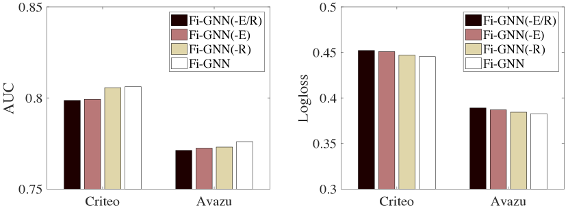
(a) edge-wise interaction (E) and residual connections (R)

(b) attentional edge weight (W) and edge-wise transformation (T)

Figure 3. Two groups of ablation studies on Fi-GNN.

4.2. Model Comparison (RQ1)

The performance of different methods is summarized in Table 2, from which we can obtain the following observations:

• LR achieves the worst performance among these baselines, which proves that the individual features is insufficient in CTR prediction.

• FM and AFM, which model second-order feature interactions, outperform LR on all datasets, indicating that it’s effective to model pair-wise interaction between feature fields. In addition, AFM achieves better performance than FM, which proves the effectiveness of attention on different interactions.

• The methods modeling high-order interaction mostly outperform the methods that model second-order interactions. This indicates the second-order feature interactions is not sufficient.

• DeepCrossing outperforms NFM, proving the effectiveness of residual connections in CTR prediction.

• Our proposed Fi-GNN achieves best performance among all these methods on two datasets. Considering the fact that previous improvements with respect to AUC at 0.001-level are regarded significant for CTR prediction task, our proposed method shows great superiority over these state-of-the-arts especially on Criteo dataset, owing to the great representative power of graph structure and the effectiveness of GNN on modeling node interactions.

• Compared with these baselines, the relative improvement of our model achieves on Criteo dataset is higher than that on Avazu dataset. This might be attributed to that there are more feature fields in Criteo dataset, which can take more advantage of the representative power of graph structure.

4.3. Ablation Study (RQ2)

Our proposed model Fi-GNN is based on GGNN, upon which we mainly make two improvements: (1) we achieve edge-wise node interactions via attentional edge weights and edge-wise transformation; (2) we introduce extra residual connections to update state along with GRU. To evaluate the effectiveness of the two improvements on modeling node interactions, we conduct ablation study and compare the following three variants of Fi-GNN:

Fi-GNN(-E/R): Fi-GNN without the two above mentioned improvements: edge-wise node interactions (E) and residual connections (R).

Fi-GNN(-E): Fi-GNN without edge-wise interactions (E).

Fi-GNN(-R): Fi-GNN without residual connections (R), which is also GGNN with edge-wise interactions.

The performance comparison is shown in Figure 3(a), from which we can obtain the following observations:

• Compared with FiGNN，the performance of Fi-GNN(-E) drops by a large margin, suggesting that it’s crucial to model the edge-wise interaction. Fi-GNN(-E) achieves better performance than Fi-GNN(-E/R), proving that the residual connections can indeed provide useful information.

• The full model Fi-GNN outperforms the three variants, indicating that the two improvements we make, i.e., residual connections and edge-wise interactions, can jointly boost the performance.

We take two measures to achieve edge-wise node interactions in Fi-GNN: attentional edge weight (W) and edge-wise transformation (T). To further investigate where dose the great improvement come from, we conduct another ablation study and compare the following three variants of Fi-GNN:

Fi-GNN(-W/T): Fi-GNN without self-adaptive adjacency matrix (W) and edge-wise transformation (T), i.e., uses binary adjacency matrix (all the edge weights are 1) and a shared transformation matrix on all the edges. It is also Fi-GNN-(E),

Fi-GNN(-W): FI-GNN without attentional edge weights, i.e., uses binary adjacency matrix.

Fi-GNN(-T): FI-GNN without edge-wise transformation, i.e., uses a shared transformation on all the edges.

The performance comparison is shown in Figure 3(a). We can see that Fi-GNN(-T) and Fi-GNN(-W) both outperform Fi-GNN(-W/T), which proves their effectiveness. Nevertheless, Fi-GNN(-W) achieves greater improvements than Fi-GNN(-T), suggesting that the edge-wise transformation is more effective than attentional edge weights in modeling edge-wise interaction. This is quite reasonable since the transformation matrix oughts to have stronger influence on interactions than a scalar attentional edge weight. In addition, Fi-GNN achieves the best performance demonstrates that it’s crucial to take both the two measures to model edge-wise interaction.

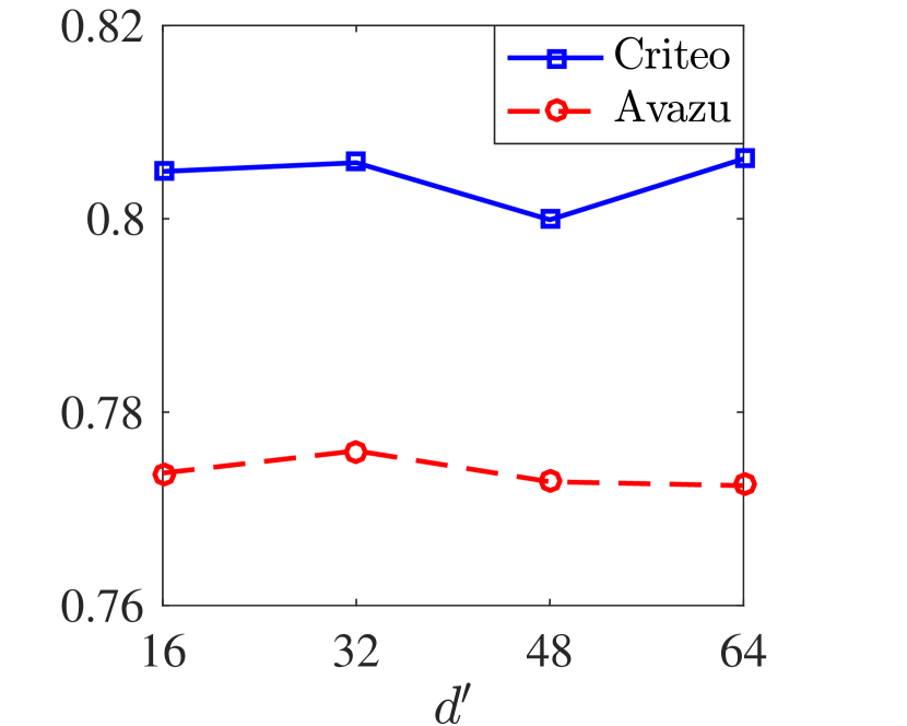
(a) State Dimensionality

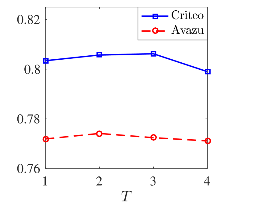
(b) Interaction Step

Figure 4. AUC performance with different state dimensionality $D$ (left) and interaction step $T$ (right) on Criteo and Avazu dataset.

4.4. Hyper-Parameter Study (RQ3)

4.4.1. Influence of different state dimensionality.

We first investigate how the performance changes w.r.t. the dimension of the node states $d^{\prime}$, which is also the output size of the initial multi-head self-attention layer. The results on Criteo and Avazu datasets are shown in Figure 4(a). On Avazu dataset, the performance first increases and then begins to decrease when the dimension size reaches 32, which indicates that state size of 32 has been represented enough information and the model is overfitted when too many parameters are used. Nevertheless, on Criteo dataset, the performance peaks with the dimension size of 64, which is reasonable since the dataset is more complexed which needs larger dimension size to carry out enough information.

4.4.2. Influence of different interaction steps.

We are interested in what the optimal highest order of feature interactions is. Our proposed Fi-GNN can answer the question, since the interaction step $T$ equals to the highest order of feature interaction. Therefore, we conduct experiments on how the performance changes w.r.t. the highest order of feature interaction, i.e., the interaction step $T$. The results on Criteo and Avazu datasets are shown in Figure 4(b). On Avazu datasets, we can see that the performance increases along with the increasing of $T$ until it reaches 2, after that the performance starts to decrease. By contrast, the performance peaks when $T=3$ on Criteo dataset. This finding suggests 2-order and 3-order interactions are enough for Avazu and Criteo dataset, respectively. It is reasonable since the Avazu and Criteo datasets have 23 and 39 feature fields, respectively. Thus the Criteo dataset needs more interaction steps for the field nodes to fully interact with other nodes in the feature graphs.

4.5. Model Explanation (RQ4)

In this section, we will answer the question that can Fi-GNN provide explanations. We apply attention mechanisms on the edges and nodes in the feature graphs and obtain attentional edge weights and attentional node weights respectively, which can provide explanations from different aspects.

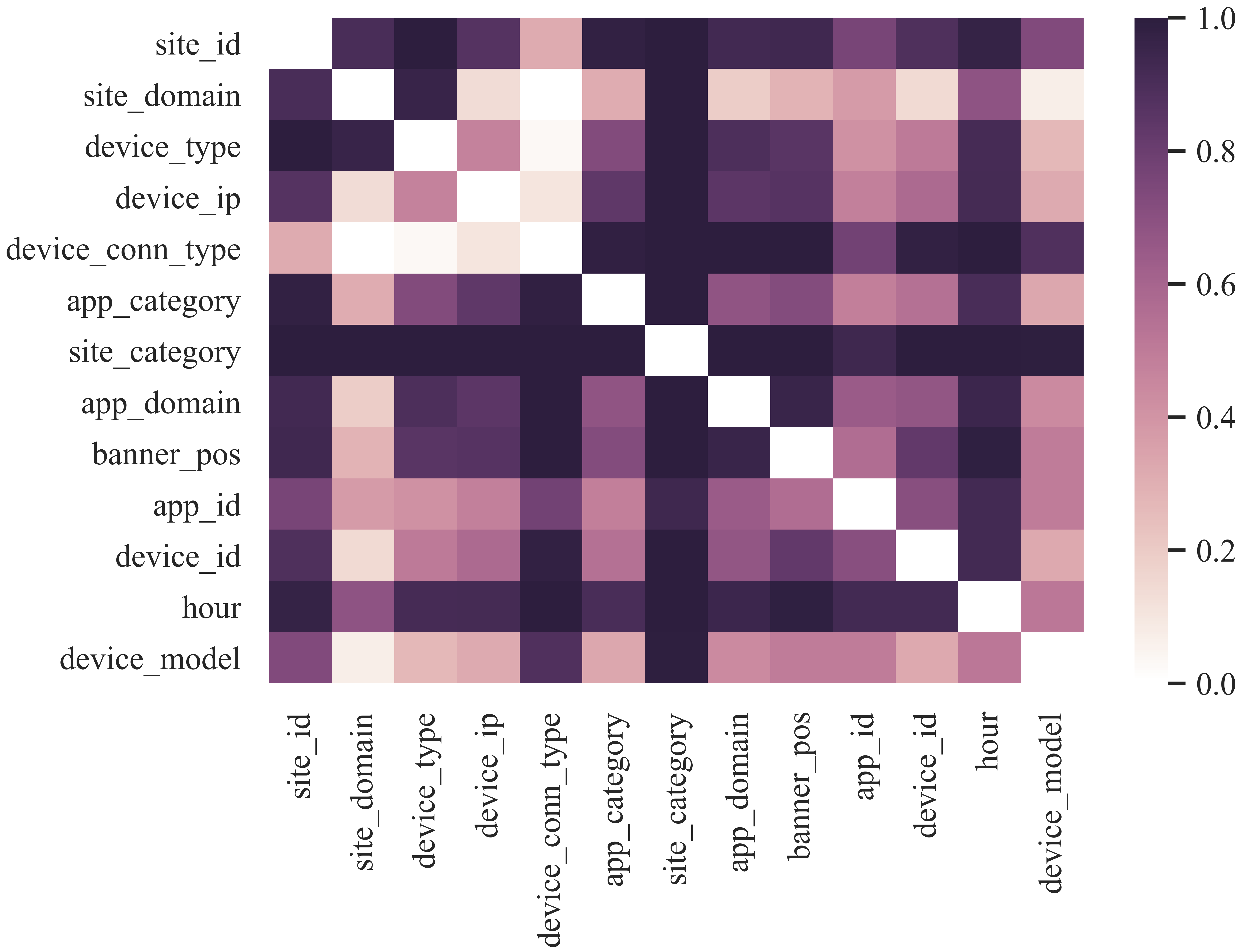
Figure 5. Heat map of attentional edge weights at the global-level on Avazu, which reflects the importance of relations between different feature fields.

4.5.1. Attentional Edge weights.

The attentional edge weight reflects the importance of interaction between the two connected field nodes, which can also reflect the relation of the two feature fields. Higher the weight is, stronger the relation is. Figure 5 presents the heat map of the globally averaged adjacency matrix of all the samples in Avazu dataset, which can reflect the relations between different fields in a global level. Since they are some anonymous feature fields, we only show the remaining 13 feature fields with real meanings.

As can be seen, some feature fields tend to have a strong relations with others, such as site_category and site_id. This makes sense since the two feature field both corresponds to the website where the impressions are put on. They contain the main contextual information of impressions. Hour is another feature which have close relations with others. It is reasonable since Avazu focuses on mobile scene, where user surfing online at any time of a day. The surfing time has strong influence on other advertising features. On the other hand, device_ip and device_id seem to have weak relations with other feature fields. This may due to that they nearly equal to user identity, which is relatively fixed and hard to be influenced by other features.

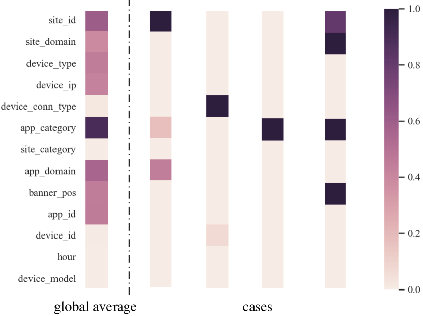
Figure 6. Heat map of attentional node weights at both global- and case-level on Avazu, which reflects the importance of different feature fields on the final prediction.

4.5.2. Attentional Node weights.

The attentional node weights reflect the importances of feature fields’ influence on the overall prediction score. Figure 6 presents the heat map of global-level and case-level attentional node weights. The leftmost is an globally averaged one of all the samples in Avazu dataset. The left four are randomly selected, whose predicted scores are $[0.97,0.12,0.91,0.99]$, and labels are $[1,0,1,1]$ respectively. At the global level, we can see that the feature field app_category have the strongest influence on the clicking behaviors. It is reasonable since Avazu focuses on mobile scene, where the app is the most important factor. At the case level, we observe that the final clicking behavior mainly depends on one critical feature field in most cases.

5. Conclusions

In this paper, we point out the limitations of the previous CTR models which consider multi-field features as an unstructured combination of feature fields. To overcome these limitations, we propose to represent the multi-field features in a graph structure for the first time, where each node corresponds to a feature field and different fields can interact through edges. Therefore, modeling feature interactions can be converted to modeling node interaction on the graph. To this end, we design a novel model Fi-GNN which is able to model sophisticated interactions among feature fields in a flexible and explicit fashion. Overall, we propose a new paradigm of CTR prediction: represent multi-field features in a graph structure and convert the task of modeling feature interactions to modeling node interactions on graphs, which may motivate the future work in this line.

- (1)
- Beck et al. (2018) Daniel Beck, Gholamreza Haffari, and Trevor Cohn. 2018. Graph-to-sequence learning using gated graph neural networks. arXiv preprint arXiv:1806.09835 (2018).
- Cheng et al. (2016) Heng-Tze Cheng, Levent Koc, Jeremiah Harmsen, Tal Shaked, Tushar Chandra, Hrishi Aradhye, Glen Anderson, Greg Corrado, Wei Chai, Mustafa Ispir, et al. 2016. Wide & deep learning for recommender systems. In Proceedings of the 1st workshop on deep learning for recommender systems. ACM, 7–10.
- Cho et al. (2014) Kyunghyun Cho, Bart Van Merriënboer, Caglar Gulcehre, Dzmitry Bahdanau, Fethi Bougares, Holger Schwenk, and Yoshua Bengio. 2014. Learning phrase representations using RNN encoder-decoder for statistical machine translation. arXiv preprint arXiv:1406.1078 (2014).
- Cui et al. (2019) Zeyu Cui, Zekun Li, Shu Wu, Xiaoyu Zhang, and Liang Wang. 2019. Dressing as a Whole: Outfit Compatibility Learning Based on Node-wise Graph Neural Networks. arXiv preprint arXiv:1902.08009 (2019).
- Grover and Leskovec (2016) Aditya Grover and Jure Leskovec. 2016. node2vec: Scalable feature learning for networks. In Proceedings of the 22nd ACM SIGKDD international conference on Knowledge discovery and data mining. ACM, 855–864.
- Guo et al. (2017) Huifeng Guo, Ruiming Tang, Yunming Ye, Zhenguo Li, and Xiuqiang He. 2017. DeepFM: a factorization-machine based neural network for CTR prediction. In Proceedings of the 26th International Joint Conference on Artificial Intelligence. AAAI Press, 1725–1731.
- Hamilton et al. (2017) Will Hamilton, Zhitao Ying, and Jure Leskovec. 2017. Inductive representation learning on large graphs. In Advances in Neural Information Processing Systems. 1024–1034.
- He and Chua (2017) Xiangnan He and Tat-Seng Chua. 2017. Neural factorization machines for sparse predictive analytics. In Proceedings of the 40th International ACM SIGIR conference on Research and Development in Information Retrieval. ACM, 355–364.
- Juan et al. (2016) Yuchin Juan, Yong Zhuang, Wei-Sheng Chin, and Chih-Jen Lin. 2016. Field-aware factorization machines for CTR prediction. In Proceedings of the 10th ACM Conference on Recommender Systems. ACM, 43–50.
- Kipf and Welling (2016) Thomas N Kipf and Max Welling. 2016. Semi-supervised classification with graph convolutional networks. arXiv preprint arXiv:1609.02907 (2016).
- Li et al. (2017) Ruiyu Li, Makarand Tapaswi, Renjie Liao, Jiaya Jia, Raquel Urtasun, and Sanja Fidler. 2017. Situation recognition with graph neural networks. In Proceedings of the IEEE International Conference on Computer Vision. 4173–4182.
- Li et al. (2015) Yujia Li, Daniel Tarlow, Marc Brockschmidt, and Richard Zemel. 2015. Gated graph sequence neural networks. arXiv preprint arXiv:1511.05493 (2015).
- Li et al. (2019) Zekun Li, Zeyu Cui, Shu Wu, Xiaoyu Zhang, and Liang Wang. 2019. Semi-Supervised Compatibility Learning Across Categories for Clothing Matching. In 2019 IEEE International Conference on Multimedia and Expo (ICME). IEEE, 484–489.
- Li et al. (2018) Zhongyang Li, Xiao Ding, and Ting Liu. 2018. Constructing Narrative Event Evolutionary Graph for Script Event Prediction. arXiv preprint arXiv:1805.05081 (2018).
- Lian et al. (2018) Jianxun Lian, Xiaohuan Zhou, Fuzheng Zhang, Zhongxia Chen, Xing Xie, and Guangzhong Sun. 2018. xDeepFM: Combining explicit and implicit feature interactions for recommender systems. In Proceedings of the 24th ACM SIGKDD International Conference on Knowledge Discovery & Data Mining. ACM, 1754–1763.
- Liu et al. (2015) Qiang Liu, Feng Yu, Shu Wu, and Liang Wang. 2015. A convolutional click prediction model. In Proceedings of the 24th ACM international on conference on information and knowledge management. ACM, 1743–1746.
- Marino et al. (2017) Kenneth Marino, Ruslan Salakhutdinov, and Abhinav Gupta. 2017. The More You Know: Using Knowledge Graphs for Image Classification. In 2017 IEEE Conference on Computer Vision and Pattern Recognition (CVPR). IEEE, 20–28.
- Mikolov et al. (2013) Tomas Mikolov, Ilya Sutskever, Kai Chen, Greg S Corrado, and Jeff Dean. 2013. Distributed representations of words and phrases and their compositionality. In Advances in neural information processing systems. 3111–3119.
- Perozzi et al. (2014) Bryan Perozzi, Rami Al-Rfou, and Steven Skiena. 2014. Deepwalk: Online learning of social representations. In Proceedings of the 20th ACM SIGKDD international conference on Knowledge discovery and data mining. ACM, 701–710.
- Qi et al. (2017) Xiaojuan Qi, Renjie Liao, Jiaya Jia, Sanja Fidler, and Raquel Urtasun. 2017. 3d graph neural networks for rgbd semantic segmentation. In Proceedings of the IEEE International Conference on Computer Vision. 5199–5208.
- Qu et al. (2016) Yanru Qu, Han Cai, Kan Ren, Weinan Zhang, Yong Yu, Ying Wen, and Jun Wang. 2016. Product-based neural networks for user response prediction. In 2016 IEEE 16th International Conference on Data Mining (ICDM). IEEE, 1149–1154.
- Qu et al. (2018) Yanru Qu, Bohui Fang, Weinan Zhang, Ruiming Tang, Minzhe Niu, Huifeng Guo, Yong Yu, and Xiuqiang He. 2018. Product-Based Neural Networks for User Response Prediction over Multi-Field Categorical Data. ACM Transactions on Information Systems (TOIS) 37, 1 (2018), 5.
- Rendle (2010) Steffen Rendle. 2010. Factorization machines. In 2010 IEEE International Conference on Data Mining. IEEE, 995–1000.
- Scarselli et al. (2009) Franco Scarselli, Marco Gori, Ah Chung Tsoi, Markus Hagenbuchner, and Gabriele Monfardini. 2009. The graph neural network model. IEEE Transactions on Neural Networks 20, 1 (2009), 61–80.
- Shan et al. (2016) Ying Shan, T Ryan Hoens, Jian Jiao, Haijing Wang, Dong Yu, and JC Mao. 2016. Deep crossing: Web-scale modeling without manually crafted combinatorial features. In Proceedings of the 22nd ACM SIGKDD International Conference on Knowledge Discovery and Data Mining. ACM, 255–262.
- Song et al. (2018) Weiping Song, Chence Shi, Zhiping Xiao, Zhijian Duan, Yewen Xu, Ming Zhang, and Jian Tang. 2018. AutoInt: Automatic Feature Interaction Learning via Self-Attentive Neural Networks. arXiv preprint arXiv:1810.11921 (2018).
- Tang et al. (2015) Jian Tang, Meng Qu, Mingzhe Wang, Ming Zhang, Jun Yan, and Qiaozhu Mei. 2015. Line: Large-scale information network embedding. In Proceedings of the 24th international conference on world wide web. International World Wide Web Conferences Steering Committee, 1067–1077.
- Tieleman and Hinton (2012) Tijmen Tieleman and Geoffrey Hinton. 2012. Lecture 6.5-rmsprop: Divide the gradient by a running average of its recent magnitude. COURSERA: Neural networks for machine learning 4, 2 (2012), 26–31.
- Vaswani et al. (2017) Ashish Vaswani, Noam Shazeer, Niki Parmar, Jakob Uszkoreit, Llion Jones, Aidan N Gomez, Łukasz Kaiser, and Illia Polosukhin. 2017. Attention is all you need. In Advances in neural information processing systems. 5998–6008.
- Veličković et al. (2017) Petar Veličković, Guillem Cucurull, Arantxa Casanova, Adriana Romero, Pietro Lio, and Yoshua Bengio. 2017. Graph attention networks. arXiv preprint arXiv:1710.10903 (2017).
- Wang et al. (2017) Ruoxi Wang, Bin Fu, Gang Fu, and Mingliang Wang. 2017. Deep & cross network for ad click predictions. In Proceedings of the ADKDD’17. ACM, 12.
- Wu et al. (2018) Shu Wu, Yuyuan Tang, Yanqiao Zhu, Xing Xie, and Tieniu Tan. 2018. Session-based Recommendation with Graph Neural Networks. In Thirty-Third AAAI Conference on Artificial Intelligence.
- Wu et al. (2019) Zonghan Wu, Shirui Pan, Fengwen Chen, Guodong Long, Chengqi Zhang, and Philip S Yu. 2019. A comprehensive survey on graph neural networks. arXiv preprint arXiv:1901.00596 (2019).
- Xiao et al. (2017) Jun Xiao, Hao Ye, Xiangnan He, Hanwang Zhang, Fei Wu, and Tat-Seng Chua. 2017. Attentional factorization machines: Learning the weight of feature interactions via attention networks. arXiv preprint arXiv:1708.04617 (2017).
- Zhang et al. (2016) Weinan Zhang, Tianming Du, and Jun Wang. 2016. Deep Learning over Multi-field Categorical Data: A Case Study on User Response Prediction. arXiv preprint arXiv:1601.02376 (2016).
- Zhou et al. (2018) Jie Zhou, Ganqu Cui, Zhengyan Zhang, Cheng Yang, Zhiyuan Liu, and Maosong Sun. 2018. Graph neural networks: A review of methods and applications. arXiv preprint arXiv:1812.08434 (2018).