Towards Amplituhedron via One-Dimensional Theory

Abstract

Inspired by the closed contour of momentum conservation in an interaction, we introduce an integrable one-dimensional theory that underlies some integrable models such as the Kadomtsev-Petviashvili (KP)-hierarchy and the amplituhedron. In this regard, by defining the action and partition function of the presented theory, while introducing a perturbation, we obtain its scattering matrix (S-matrix) with Grassmannian structure. This Grassmannian corresponds to a chord diagram, which specifies the closed contour of the one-dimensional theory. Then, we extract a solution of the KP-hierarchy using the S-matrix of theory. Furthermore, we indicate that the volume of phase-space of the one-dimensional manifold of the theory is equal to a corresponding Grassmannian integral. Actually, without any use of supersymmetry, we obtain a sort of general structure in comparison with the conventional Grassmannian integral and the resulted amplituhedron that is closely related to the Yang-Mills scattering amplitudes in four dimensions. The proposed theory is capable to express both the tree- and loop-levels amplituhedron (without employing hidden particles) and scattering amplitude in four dimensions in the twistor space as particular cases.

I Introduction

One of the key points to understand particle physics is the scattering amplitudes. On the other hand, the standard method of calculating these scattering amplitudes is to apply the Feynman diagrams, which have many complications Kampf-2013 ; Elvang-2015 ; Kampf-2019 . These complications have always been a motivation for physicists to simplify their calculations. A specific example of such efforts is the Park-Taylor formula, which describes the interaction between gluons Parke-1986 ; Mangano-1991 .

As another example, in Ref. Britto-2005 , it has been shown that one can, with correct factorization, give a recursive expression in terms of amplitudes with less external particles, in which a scattering amplitude is broken down into simpler amplitudes. Also recently, in Ref. Arkani-Hamed-2014 , by employing the recursive expression used in Ref. Britto-2005 and the twistor theory, a geometric structure has been proposed that is coined amplituhedron. This structure enables simplification of the computation of scattering amplitudes in some quantum field theories such as super-Yang-Mills theory. The amplituhedron challenges spacetime locality and unitarity as chief ingredients of the standard field theory and the Feynman diagrams. Hence, due to spacetime challenges at the scale of quantum gravity Callender-2001 and since locality will have to be remedied if gravity and quantum mechanics ought to coexist, the amplituhedron is of much interest. However, the presented amplituhedron requires supersymmetry and introduces the scattering amplitude of massless particles, nevertheless no trace of supersymmetry has been seen up to now, and also each material particle has mass. On the other hand, it has not been specified/discussed why the number of dimensions should be exactly four in the amplituhedron and, in general, the scattering amplitude issues.

In this work, we show that interesting integrable models can have a common foundation and being raised from a single root. For this purpose, inspired by the fact that geometric representation of the momentum conservation of participated particles in an interaction leads to the formation of a closed contour, we introduce a theory in one dimension that underlies some integrable models in various dimensions. The important kinds of integrable models that we are considering here are the KP-hierarchy Jimbo-1983 , two-dimensional models Ishibashi-1987 ; Vafa-1987 ; Verlinde-1987 , the amplituhedron Arkani-Hamed-2014 . In the proposed theory, as there is only one dimension, in analogy with the closed contour resulted from the momentum conservation, there is only one point that evolves in itself, hence we refer to this theory as a point theory (PT).

In the following, we first define the corresponding action, and then its equation of state and path integral. Also, we present a specific symmetry of the PT. Afterward, by defining S-matrix of the PT, we show the Grassmannian structure of the S-matrix of the PT, and in turn, we specify its closed contour. Thereupon, we define a hierarchy transformation by which, we represent some integrable models based on the PT. Thus, we express a vacuum solution in the PT as a solution of the KP-hierarchy. Accordingly, under these considerations, we endeavor to move towards the amplituhedron without employing supersymmetry. For this purpose, we indicate the tree and loop levels of the amplituhedron as special cases of the contour integrations of the volume of phase-space of the closed contour, wherein the volume itself is as a Grassmannian integral. Finally, we discuss the physical meaning and importance of the linked closed contour.

II Foundation of Point Theory

It is convenient to work in the natural units (i.e., $c=1=\hbar$) with an action on a real $1$-dimensional compact Hausdorff manifold, say $\mathcal{C}$ as a vacuum, namely

$$S=\frac{1}{\kappa}\oint_{\mathcal{C}}dS(z)\equiv-\frac{1}{\kappa}\oint_{\mathcal{C}}\psi(z)\varphi(z)dz,$$ (1)

where $\psi(z)$ and $\varphi(z)$ are two fermionic fields over the manifold, $\kappa$ is a constant and $z$ is the parameter of the manifold $\mathcal{C}$.

Each real $1$-dimensional compact Hausdorff manifold (e.g., knots and links), generally, has its own global topological properties. For instance, one of these features has been expressed in the Fary-Milnor theorem Sullivan-2008 , which (using a specified local scalar curvature at any point on the curve) explains whether or not a $1$-dimensional manifold is a knot. However, global topological properties of compact manifolds cannot be determined by local coordinates. For this reason, non-local or higher-dimensional coordinates, e.g. complex numbers, can be used instead of real local coordinates to express the global properties.

Therefore, if the corresponding manifold is a circle, as real projective line, then its corresponding parameter will at least be a unit complex number. In the case that the manifold $\mathcal{C}$ is an unknot and unlinked disconnected compact manifold (e.g., several circles), then the parameter $z$ can at least be a complex number. Also, it is known that a knot is an embedding of a circle into $3$-dimensional Euclidean space $\mathbb{R}^{3}$ Cromwell-2004 and $\mathbb{R}^{3}$ is a subspace of $1$-dimensional biquaternion space. Now, if the manifold $\mathcal{C}$ is a knotted and/or a linked one, then its parameter $z$ will be a member of a special subspace (say, $\mathbf{M}$, which corresponds to Minkowski space wherein $\mathbb{R}^{3}\subset\mathbf{M}$) of biquaternion space having $Q^{*}=Q^{\star}$, with an additional constraint on the $\mathbf{M}$. An additional constraint is required because the subspace $\mathbf{M}$ corresponds to $4$-dimensional Minkowski space that has one dimension more than $\mathbb{R}^{3}$.

Before we determine such a constraint, first we write each number of the subspace $\mathbf{M}$ (say, $Q$) in the unitary matrix representation in terms of the Euler parameters, namely

$$Q=\begin{pmatrix}a_{0}+ia_{3}&ia_{1}+a_{2}\\[3.00003pt] ia_{1}-a_{2}&a_{0}-ia_{3}\end{pmatrix}.$$ (2)

In this way, due to the twistor theory Huggett-1994 , each point (number) in the subspace $\mathbf{M}$ determines a line in the null projective twistor space, in which each twistor, say $\varpi$, has coordinates $\varpi\equiv((\zeta_{1},\zeta_{2}),(\zeta_{3},\zeta_{4}))\equiv(\lambda,\mu)$. Also, one can specify a point in the null projective twistor space by two points or a null line in the $\mathbf{M}$. Second, we determine $n$ different values of the parameter $z$, as different numbers (points) $z_{i}\in\mathbf{M}$ for $i=1,\cdots,n$, which fix the manifold $\mathcal{C}$ (see, e.g., Fig. $1$). Now, due to

$$\begin{cases}\lambda_{i}z_{i}=\mu_{i}\\ \lambda_{i}z_{i+1}=\mu_{i}\end{cases}\qquad\mathrm{and}\qquad\begin{cases}\lambda_{i}z_{i}=\mu_{i}\\ \lambda_{i+1}z_{i}=\mu_{i+1},\end{cases}$$ (3)

we choose the constraint such a way that

$$||(z_{i}-z_{i+1})||^{2}\equiv(z_{i}-z_{i+1})(z_{i}-z_{i+1})^{\star}=0.$$ (4)

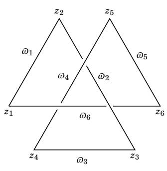
Figure 1: A $1$-dimensional manifold in $\mathbf{M}$.

As mentioned earlier, the 1-dimensional manifold corresponds to the closed contour resulted from the momentum conservation of participated particles in an interaction. In this regard, the closed contour can be considered as a knot, and hence, the topological properties of the knot can be related to some of the interaction properties. On the other hand, the closed contour can be a link. However in this research, we explain the basis of the PT and its relation with the scattering amplitude and amplituhedron, and will examine the characteristics of the states as knot and link in another research. Nevertheless, in the following, we briefly discuss the physical interpretation of the states as linked closed contour.

The variation of action (1) gives two trivial solutions

$$\frac{\delta\partial_{z}S(z)}{\delta\varphi(z)}=0=\frac{\delta\partial_{z}S(z)}{\delta\psi(z)}\ \Rightarrow\ \psi(z)=0=\varphi(z),$$ (5)

as the Euler-Lagrange equations. However, there is also a non-trivial solution that, without loss of generality about the constant of integration, can set to be

$$\delta\partial_{z}S(z)=0\Longrightarrow\psi(z)\varphi(z)=1.$$ (6)

This solution is the continuity equation in one dimension wherein $\psi(z)\varphi(z)$ is the conserved current within it. Considering the non-trivial case, we choose an arbitrary solution

$$\psi(z)\equiv e^{S(z)}\xRightarrow{\eqref{eq-of-mo}}\varphi(z)=e^{-S(z)},$$ (7)

which, after quantization, it will be clear that is a good choice. Also, as there is no derivative of the field in the Lagrangian, the field momentum is zero. Thus, the energy density is

$$h(z)=\psi(z)\varphi(z),$$ (8)

which, due to Eq. (6), is a constant. Also, for later on uses, we expand $\psi(z)$ and $\varphi(z)$ as

$$\psi(z)=\sum\limits_{p\in\mathbb{Z}+1/2}\psi_{p}z^{-(p+1/2)},$$ (9)

$$\varphi(z)=\sum\limits_{p\in\mathbb{Z}+1/2}\varphi_{p}z^{-(p+1/2)},$$ (10)

where $\psi_{p}$ and $\varphi_{p}$ are coefficients of the expansion.

At this stage, similar to complex numbers, we extend the Cauchy integral theorem to any biquaternion number $z\in\mathbf{M}$. In this regard, for each real number $l\neq 1$, we have

$$\oint_{\mathcal{C}}z^{-l}dz=-(l-1)^{-1}\oint_{\mathcal{C}}d(z^{-l+1})\mathrel{\mathop{=}^{l\neq 1}}0.$$ (11)

When $l=1$, it is known that one can write the point $z$ with arbitrary parameters $x,y\in\mathbb{R}$ as

$$z=x+y\mathbf{n},$$ (12)

where $\mathbf{n}=\sum_{i=1}^{3}a_{i}e_{i}$ with $\mathbf{n}^{2}=1$. In this case, using the Stokes-Cartan theorem cartan–1945 , the Wick rotation method Wick ; Peskin , and transformations $\mathbf{i}=-h\mathbf{n}$ and $\bar{y}=hy$, wherein $h^{2}=-1$, then $z=x+\bar{y}\mathbf{i}$. Hence, we get

$$\begin{split}&\oint_{\mathcal{C}}z^{-1}dz=\int_{\mathcal{S}}dzdz^{\star}\partial_{z^{\star}}\partial_{z}\ln{z}\\ &=\int_{\mathcal{S}-\mathcal{S}_{0}}\!\!\!\!\!\!\!dzdz^{\star}\partial_{z^{\star}}\partial_{z}\ln{z}+\oint_{\mathcal{C}_{0}}z^{-1}dz,\end{split}$$ (13)

where $\mathcal{S}$ is the Seifert surface that corresponds to the closed curve $\mathcal{C}$ containing the point $z=0$, $\mathcal{S}_{0}$ is the infinitesimal closed neighborhood of $z=0$ in the Seifert surface, and $\mathcal{C}_{0}$ is the boundary of $\mathcal{S}_{0}$. As $\partial_{z^{\star}}\partial_{z}\ln{z}$ on the surface $\mathcal{S}-\mathcal{S}_{0}$ is zero, its integration over the surface $\mathcal{S}-\mathcal{S}_{0}$ vanishes. Therefore, the only remaining term of relation (13), as a contour integration over a general closed contour (e.g., knotted or linked closed contour), is the last term. That is, we have Gentili-2007

$$\oint_{\mathcal{C}}z^{-1}dz=\oint_{\mathcal{C}_{0}}z^{-1}dz=2\pi\mathbf{i}_{0},$$ (14)

where, by $\mathbf{i}_{0}$, we mean a specific choice of $\mathbf{i}$ that, without loss of generality, we choose it to be $\mathbf{i}_{0}=e_{1}$.

Accordingly, by employing (1), (9) and (14), the corresponding path integral of the PT can be written as

$$\mathcal{Z}=\int D\psi D\varphi\;e^{\sum\limits_{p}\psi_{p}\varphi_{p}},$$ (15)

where we have set the constant $\kappa$ in action (1) equal to $2\pi e_{1}$, $D\psi=\prod\limits_{p\in\mathbb{Z}+1/2}d\psi_{p}$ and $D\varphi=\prod\limits_{p\in\mathbb{Z}+1/2}d\varphi_{p}$. Then, using the path integral (15) and the Berezin integral Berezin-1966 , we can calculate the many-point correlation function. Alternatively, to calculate the many-point correlation function, we can use the canonical quantization of $\psi_{p}$ and $\varphi_{p}$. In this way, we have the Clifford algebra with fermionic operators $\hat{\psi}_{p}$ and $\hat{\varphi}_{p}$ that satisfy the anti-commutators

$$\{\hat{\psi}_{p},\hat{\psi}_{q}\}=0,\quad\{\hat{\varphi}_{p},\hat{\varphi}_{q}\}=0\quad{\rm and}\quad\{\hat{\psi}_{p},\hat{\varphi}_{q}\}=\delta_{p,-q},$$ (16)

where $p$ and $q\in\mathbb{Z}+1/2$. To give a representation of this algebra, we define the vacuum state as

$$\hat{\psi}_{p}|0_{\mathcal{C}}>=0\;\;(p>0),\;\;\hat{\varphi}_{p}|0_{\mathcal{C}}>=0\;\;(p>0),$$ (17)

$$<0_{\mathcal{C}}|\hat{\psi}_{p}=0\;\;(p<0),\;\;<0_{\mathcal{C}}|\hat{\varphi}_{p}=0\;\;(p<0).$$ (18)

Using quantum forms of expansions (9), the quantum form of the Lagrangian is

$$\partial_{z}\hat{S}(z)=-\sum\limits_{l\in\mathbb{Z}}\hat{S}_{l-1}z^{-l},$$ (19)

where

$$\hat{S}_{l-1}=\sum\limits_{p\in\mathbb{Z}+1/2}:\hat{\psi}_{p}\hat{\varphi}_{l-p-1}:,$$ (20)

and it is compatible Miwa-2000 with the quantum forms of solutions (7), namely

$$\hat{\psi}(z)=:e^{\hat{S}(z)}:\quad{\rm and}\quad\ \hat{\varphi}(z)=:e^{-\hat{S}(z)}:.$$ (21)

In the above relations, $:\hat{a}\hat{b}:$ is the normal ordered form of $\hat{a}\hat{b}$.

Symmetry of Point Theory:  According to solutions (21), the field $\hat{\psi}(z)$ is equal to its partition function. Thus, due to the quantization process, it means that the theory will not change after quantization. This symmetry is a special feature of the PT that results the uniformity of physics in large and small scales. For instance, the result of such a symmetry makes the physics of a statistical set of leptons and quarks being similar to physics of each one of those.

III S-Matrix and Grassmannian Structure

To express the S-matrix, as an evolution operator for initial state $|i_{\mathcal{C}}>$ and final state $|f_{\mathcal{C}}>$ while using the free Hamiltonian and relations (1), (11), (14) and (19), we obtain

$$\mathbb{S}_{if}\!\!=<\!i_{\mathcal{C}}|\!:\!e^{-\frac{1}{\kappa}\oint_{\mathcal{C}}\hat{\psi}(z)\hat{\varphi}(z)dz}\!:\!|f_{\mathcal{C}}\!>=<\!i_{\mathcal{C}}|\!:\!e^{\hat{S}_{0}}\!:\!|f_{\mathcal{C}}\!>.$$ (22)

In other words, using relations (16) and (20), one equivalently gets

$$:\!e^{\frac{1}{\kappa}\oint_{\mathcal{C}}\hat{\psi}(z)\check{\varphi}(z)dz}\!:\hat{\psi}(z^{\prime}):\!e^{-\frac{1}{\kappa}\oint_{\mathcal{C}}\hat{\psi}(z)\hat{\varphi}(z)dz}\!:=e\,\hat{\psi}(z^{\prime}),$$ (23)

where $e$ is the Euler number. That is, we have a trivial case wherein the initial and final states are the same. However, adding a perturbation to the free Hamilton results a general nontrivial expression for the S-matrix in the PT, wherein the initial state evolves. In this respect, we define a perturbed Hamiltonian as the interaction of superposition of $n$ specific points of $\mathcal{C}$ with the other points, namely

$$\begin{split}\hat{\psi}(z)&\hat{\varphi}(z)\rightarrow\hat{\psi}(z)\hat{\varphi}(z)+\\ &\iota\,C(z)\hat{\psi}(z)\big{[}\hat{\varphi}(z_{1}^{\prime})+\cdots+\hat{\varphi}(z_{n}^{\prime})\big{]},\end{split}$$ (24)

where $\iota$ is a constant and $C(z)$ for $a=1,\cdots,n$ is the probability function of interaction of $\hat{\psi}(z)$ with one or more points of $\mathcal{C}$. Accordingly, we express the S-matrix operator in terms of the Dyson series as

$$\!\hat{\mathbb{S}} = \!\!\sum\limits_{k=1}^{n}\!\frac{(\frac{\iota}{\kappa})^{k}}{k!}:\!\prod\limits^{k}_{\alpha=1}\oint_{\mathcal{C}}\!\left[\sum_{a=1}^{n}C_{\alpha}(z_{\alpha})\hat{\psi}(z_{\alpha})\hat{\varphi}(z_{a}^{\prime})\right]\!:dz_{\alpha}$$ (25)

$$\equiv \!\!\sum\limits_{k=1}^{n}\hat{\mathbb{S}}_{(k)},$$ (26)

wherein the constant $\iota$ is determined in a way that

$$<0_{\mathcal{C}}|\hat{\mathbb{S}}|0_{\mathcal{C}}\!>=1,$$ (27)

and given that the product of two identical Fermion fields is zero, then $\hat{\mathbb{S}}_{(k)}$ for $k>n$ vanishes.

Each $\hat{\mathbb{S}}_{(k)}$ is equivalent to the simultaneous interaction of $k$ ordered points of $n$ specific points $(z_{1}^{\prime},\cdots,z_{n}^{\prime})$ within $\mathcal{C}$. Also, each $\hat{\mathbb{S}}_{(k)}$ has a Grassmannian structure with a Grassmannian $G(k,n)$, say $C$, as

$$C\equiv\begin{pmatrix}C_{1}(z_{1}^{\prime})&\cdots&C_{1}(z_{n}^{\prime})\\ \vdots&\ddots&\vdots\\ C_{k}(z_{1}^{\prime})&\cdots&C_{k}(z_{n}^{\prime})\end{pmatrix},$$ (28)

in a way that $<\!0_{\mathcal{C}}|\hat{\mathbb{S}}_{(k)}|0_{\mathcal{C}}\!>$ being equal to the sum of minors of the Grassmannian $C$.

On the other hand, each minor of the Grassmannian $C$ is the probability of simultaneous interaction of $k$ specific ordered points of $(z_{1}^{\prime},\cdots,z_{n}^{\prime})$ within $\mathcal{C}$. Also, due to the conditional probability in the probability theory, the probability that each point $z_{a}^{\prime}$ of $(z_{1}^{\prime},\cdots,z_{n}^{\prime})$ interacts with the manifold in the $\alpha$’th order is

$$\bar{c}_{\alpha a}\equiv\dfrac{\det\begin{pmatrix}c_{1a}&\cdots&c_{1,a+\alpha-1}\\ \vdots&\ddots&\vdots\\ c_{\alpha a}&\cdots&c_{\alpha,a+\alpha-1}\end{pmatrix}}{\det\begin{pmatrix}c_{1a}&\cdots&c_{1,a+\alpha-2}\\ \vdots&\ddots&\vdots\\ c_{\alpha-1,a}&\cdots&c_{\alpha-1,a+\alpha-2}\end{pmatrix}},$$ (29)

where these two determinants are the probability of simultaneous interaction of $(\alpha-1)$ ordered points and the same $(\alpha-1)$ ordered points plus one extra point of $n$ specific points $(z_{1}^{\prime},\cdots,z_{n}^{\prime})$ within $\mathcal{C}$, and each $c_{\alpha a}\equiv C_{\alpha}(z_{a}^{\prime})$ is the element of the matrix $C$.

Thus, due to the number of minors of the Grassmannian $C$ (that is equal to the combination $\textbf{C}^{n}_{k}$) and given that the sum of the probabilities of all possible states of the simultaneous interaction of $k$ ordered points of $n$ specific points $(z_{1}^{\prime},\cdots,z_{n}^{\prime})$ within $\mathcal{C}$ is equal to one, by employing the Wick theorem Miwa-2000

$$<0_{\mathcal{C}}|\hat{\psi}(z_{1})\cdots\hat{\psi}(z_{n})\hat{\varphi}(z_{1}^{\prime})\cdots\hat{\varphi}(z_{n}^{\prime})|0_{\mathcal{C}}>=$$ (30)

$$\det\left(<0_{\mathcal{C}}|\hat{\psi}(z_{i})\hat{\varphi}(z_{j}^{\prime})|0_{\mathcal{C}}>\right),$$ (31)

and relations (9) and (14) that result

$$<\!0_{\mathcal{C}}|\frac{1}{\kappa}\oint_{\mathcal{C}}\hat{\psi}(z)\hat{\varphi}(z^{\prime})dz|0_{\mathcal{C}}\!>=1,$$ (32)

we obtain

$$\frac{k!}{\iota^{k}}<\!0_{\mathcal{C}}|\hat{\mathbb{S}}_{(k)}|0_{\mathcal{C}}\!>=\sum\limits_{h=1}^{\textbf{C}^{n}_{k}}M_{h}=1.$$ (33)

Furthermore, the minors $M_{h}$ of the Grassmannian $C$, as probability of simultaneous interaction of $k$ specific points of $(z_{1}^{\prime},\cdots,z_{n}^{\prime})$ within $\mathcal{C}$, are, in general, positive numbers. Therefore, the Grassmannian $C$ is a positive Grassmannian. In addition, in Ref. Kodama-2017 , it has been shown that each non-negative Grassmannian corresponds to a chord diagram. In this way, as a chord diagram is a closed contour, each non-negative Grassmannian, and in turn each $\hat{\mathbb{S}}_{(k)}$, specifies a closed contour $\mathcal{C}$. Moreover, since a Grassmannian $G(k,n)$ is a space that parameterizes all $k$-dimensional linear subspaces of the $n$-dimensional vector space, if we mod out it by the general linear group $GL(k)$, there will be no change in it. Then, dividing relation (33) by one of $M_{h}$ or a constant, makes no change in $\mathcal{C}$. Eventually, it is obvious that the S-matrix in the PT has a Grassmannian structure.

IV Hierarchy Transformation and KP-Hierarchy

To investigate the integrability and solitonic properties of the PT, we inquire relation between the PT and the KP-hierarchy. The KP-hierarchy is based on mathematical foundation in terms of a Grassmannian variety Jimbo-1983 ; Miwa-2000 ; Kodama-2017 . It is supplemented with a number of classical and non-classical reductions that contain many integrable equations and solitonic models Jimbo-1983 . Indeed, the KP-hierarchy is a hierarchy of nonlinear partial differential equations in a function, say $\tau(x)$, of infinite number of variables $x_{l}$ for $l=1,\cdots,\infty$ as hierarchy coordinates. As the KP-hierarchy is an integrable system, the plausible (physical) meaning of the hierarchy coordinates can be related to the infinite numbers of possible conserved quantities that any KP-hierarchy soliton solution can contain Kodama–2011 ; Kodama–2014 . Such a $\tau(x)$ is a function that should satisfy the bilinear identity Jimbo-1983

$$\oint_{\mathcal{C}}e^{\xi(k,x-x^{\prime})}\tau\big{(}x-\epsilon(k)\big{)}\tau\big{(}x^{\prime}+\epsilon(k)\big{)}dk\equiv 0,$$ (34)

where $\xi(k,x)\equiv\sum_{l=0}^{\infty}x_{l}k^{l}$, $k\in\mathbf{M}$ is an arbitrary point in the manifold ${\mathcal{C}}$, $\epsilon(k)\equiv\big{(}1,1/k,1/(2k^{2}),\cdots\big{)}$, and arbitrary variables $x\equiv(x_{0},x_{1},x_{2},\cdots)$ and $x^{\prime}\equiv(x^{\prime}_{0},x^{\prime}_{1},x^{\prime}_{2},\cdots)$ with $x_{l},x^{\prime}_{l}\in\mathbf{M}$.

To show the relation between the PT and the KP-hierarchy, we employ a transformation, which we will refer to it as a hierarchy transformation (HT), in the form

$$\text{HT:}\begin{cases}\hat{\psi}(z)\rightarrow e^{H(x)}\hat{\psi}(z)e^{-H(x)}\cr\hat{\varphi}(z)\rightarrow e^{H(x)}\hat{\varphi}(z)e^{-H(x)},\end{cases}$$ (35)

where

$$H(x)\equiv\oint_{\mathcal{C}}\xi(z^{\prime},x)dS(z^{\prime})/(2\pi e_{1}).$$ (36)

Given that the function $\xi(k,x)$, for constant parameters $x\equiv(x_{0},x_{1},x_{2},\cdots)$, is regular with respect to $k$, relation (36) means that the closed contour $\mathcal{C}$ in relation (1), without changing the topological properties, is subjected to a diffeomorphism as

$$\begin{split}H(x)&=-\oint_{\mathcal{C}}\xi(z^{\prime},x)dz^{\prime}\psi(z^{\prime})\varphi(z^{\prime})/(2\pi e_{1})\\ &=-\oint_{\mathcal{C}^{\prime}}dz^{\prime\prime}\psi^{\prime}(z^{\prime\prime})\varphi^{\prime}(z^{\prime\prime})/(2\pi e_{1}),\end{split}$$ (37)

where $dz^{\prime\prime}\equiv\xi(z^{\prime},x)dz^{\prime}$, $\psi^{\prime}(z^{\prime\prime})\varphi^{\prime}(z^{\prime\prime})=\psi(z^{\prime})\varphi(z^{\prime})$ and $\mathcal{C}^{\prime}$ is a diffeomorphism of $\mathcal{C}$. Hence, after some calculations Miwa-2000 , transformation (35) reads

$$\begin{cases}\hat{\psi}(z)\rightarrow e^{-\xi(z,x)}\hat{\psi}(z)\equiv\hat{\psi}(z,x)\cr\hat{\varphi}(z)\rightarrow e^{\xi(z,x)}\hat{\varphi}(z)\equiv\hat{\varphi}(z,x).\end{cases}$$ (38)

Now, we define $\hat{\mathbb{S}}_{(k,x)}$ as

$$\hat{\mathbb{S}}_{(k,x)}\!\!\equiv\!\frac{(\frac{\iota}{\kappa})^{k}}{k!}\!:\!\!\prod\limits^{k}_{\alpha=1}\!\oint_{\mathcal{C}}\!\!\left[\sum_{a=1}^{n}\!\!C_{\alpha}(z_{\alpha})\hat{\psi}(z_{\alpha},x)\hat{\varphi}(z_{a}^{\prime})\right]\!\!:\!dz_{\alpha}.$$ (39)

Since, the function $\tau(x)$, as a solution of the KP-hierarchy, is define as

$$\tau(x)=\frac{k!}{\iota^{k}}<\!0_{\mathcal{C}}|\hat{\mathbb{S}}_{(k,x)}|0_{\mathcal{C}}\!>=\mathrm{Wr}(f_{1},\cdots,f_{k}),$$ (40)

where $\mathrm{Wr}(f_{1},\cdots,f_{k})$ is the Wronskian of functions $f_{\alpha}$ for $\alpha=1,\cdots,k$ as each $f_{\alpha}$ is

$$f_{\alpha}\equiv\left(c_{\alpha 1}e^{-\xi(z_{1}^{\prime},x)},\cdots,c_{\alpha n}e^{-\xi(z_{n}^{\prime},x)}\right).$$ (41)

At this stage, as in Refs. Miwa-2000 ; Chakravarty-2014 ; Kodama-2017 , it has been shown that the $\mathrm{Wr}(f_{1},\cdots,f_{k})$ is a solution of the KP-hierarchy, thus we conclude that a vacuum solution in the PT is equivalent to a solution of the KP-hierarchy.

V Phase-Space of $\mathcal{C}$

Consider a quantum system with a Hamiltonian operator $\hat{\mathcal{H}}$ and its basis states. The time evolution of the probability of a state of the system, say $p_{i}$, in this Hamiltonian basis is

$$\partial_{t}p_{i}=i\hat{\mathcal{H}}p_{i}=i\mathcal{H}_{i}p_{i}$$ (42)

that leads to

$$d\ln{p_{i}}=i\mathcal{H}_{i}dt.$$ (43)

For a one-dimensional quantum system, relation (43) is proportional to the volume element of phase-space of the state $p_{i}$. In this way, the volume element of phase-space of total system is proportional to

$$\prod\limits_{i}d\ln{p_{i}}.$$ (44)

Inspired by this explanation, due to definition (29) and as the Grassmannian $C$ specifies the closed contour $\mathcal{C}$, we (plausibly) assume that the volume element of phase-space of the closed contour $\mathcal{C}$ is

$$\prod\limits^{k,n}_{\alpha,a=1}d\ln{\bar{c}_{\alpha a}}.$$ (45)

Then, using definition (29) and

$$M_{b}\equiv\det\begin{pmatrix}c_{1,b}&\cdots&c_{1,b+k-1}\\ \vdots&\ddots&\vdots\\ c_{kb}&\cdots&c_{k,b+k-1}\end{pmatrix},$$ (46)

expression (45) reads as

$$\dfrac{d^{k\times n}c_{\alpha a}}{\prod\limits_{b=1}^{n}M_{b}}.$$ (47)

However, there are two points that must be considered in order to define the volume element of the phase-space of $\mathcal{C}$. First, as the Grassmannian $C$ is invariant under general linear group $GL(k)$, the volume element of the phase-space of it must be mod out by $GL(k)$ ‘gauge’ redundancy. The second point is about the relation between the Grassmannian $C$ and the coordinates $z_{a}$. Given relation (3), twistors, say $\varpi_{a}=(\zeta_{a1},\cdots,\zeta_{a4})$, can correspond to the lines between two points $z_{a}$ and $z_{a-1}$ in analogy with the momentum of particles in the closed contour of momentum conservation. Accordingly, if we define

$$c_{\alpha a}\varpi_{a}\equiv y_{\alpha},$$ (48)

two different cases will be possible. One case is that the inner product of the $4$ $n$-component vector ${\bm{\varpi}}$ to each of the $k$ $n$-component row-vectors of the $C$ matrix being zero (i.e., all of $y_{\alpha}=0$). The other case is that some of $y_{\alpha}$’s being zero.

In the above first case, there would be a $(4+k)$-plane. Now, we employ some auxiliary parameters, say a matrix $\mathtt{z}$ made of elements $\mathtt{z}_{a\alpha}$, as

$$C\cdot\mathtt{z}\equiv\mathtt{y}\qquad\ \text{with constraint:}\quad\mathtt{y}=\mathbb{I}_{k\times k}.$$ (49)

Then, due to the property of the matrix $C$, this matrix $\mathtt{z}$ contains $k$ independent column-vectors, which (within the first case) are also independent from $4$ $n$-component vector $\varpi_{a}$. Accordingly, we can choose a matrix, say $Z$, consists of $n$ row-vectors $Z_{a}\equiv(\zeta_{a1},\cdots,\zeta_{a4},\mathtt{z}_{a1},...,\mathtt{z}_{ak})$, which contains $(4+k)$ independent $n$-component column-vectors as a basis for the above $(4+k)$-plane. Such a basis and the above constraint eliminate the gauge redundancy $GL(k)$. In this case, we can assume a polygon in a $(3+k)$-dimensional projective space whose $n$ vertices are $Z_{a}$’s.

At this stage, we satisfy the elimination of the gauge redundancy $GL(k)$ and also the application of those two mentioned cases (48) by imposing the Dirac delta functions to the volume element of the phase-space as

$$\dfrac{d^{k\times n}c_{\alpha a}}{\prod\limits_{b=1}^{n}M_{b}}\delta^{k\times k}\mathtt{(y-\mathbb{I}_{k\times k})}\delta^{k^{\prime}\times 4}(y-0_{k^{\prime}\times 4}).$$ (50)

Indeed, the Dirac delta functions $\delta^{k\times k}\mathtt{(y-\mathbb{I}_{k\times k})}$ eliminate the gauge redundancy $GL(k)$ and the Dirac delta functions $\delta^{k^{\prime}\times 4}(y-0_{k^{\prime}\times 4})$ impose those two mentioned cases of (48). Therefore, expression (50) indicates that the volume of the phase-space is equal to a corresponding Grassmannian integral. In addition, due to definition $M_{b}$’s in (46), the volume element, and in turn the corresponding Grassmannian integral, is obviously cyclic-invariant.

VI Four-Dimensional Tree-Amplituhedron

In this section, we endeavor to show that the volume of the phase-space of $\mathcal{C}$ is equivalent with the amplituhedron in a four-dimensional spacetime. For this propose, first we indicate that the tree-amplituhedron in a four-dimensional spacetime can be deduced from the first case of definition (48). Actually, in this case, the integration of expression (50) becomes

$$\int\dfrac{d^{k\times n}c_{\alpha a}}{\prod\limits_{b=1}^{n}M_{b}}\delta^{k\times(4+k)}(\mathtt{Y}-\mathtt{Y}_{0})\equiv\mathcal{A}_{n,k},$$ (51)

where $\mathtt{Y}$ is a $[k\times(4+k)]$-matrix generally defined as $\mathtt{Y}\equiv C\cdot Z$ with constraint $\mathtt{Y}_{0}=(0_{k\times 4},\mathbb{I}_{k\times k})$. Furthermore, consider each cell decomposition (say $T$) of the polygon with the $n$ vertices $Z_{a}$’s, which has a few cells (say $\Gamma$’s), wherein any cell of it, as a particular example with Grassmannian

$$\begin{pmatrix}c_{1,a_{(1)}}&\cdots&c_{1,a_{(4+k)}}\\ \vdots&\ddots&\vdots\\ c_{k,a_{(1)}}&\cdots&c_{k,a_{(4+k)}}\end{pmatrix},$$ (52)

is specified as

$$\mathtt{Y}_{\alpha}\equiv\sum\limits_{i=0}^{k+3}c_{\alpha,a_{(1+i)}}Z_{a_{(1+i)}}.$$ (53)

In here, $\mathtt{Y}_{\alpha}$ is $\alpha$th row-vector of the defined matrix $\mathtt{Y}$ but with $(4+k)$ components, wherein $k\times(n-k-4)$ components of the matrix $C$ have been set to be zero. Hence, using (53), each of the corresponding minors (46) and the related multiplication of differential elements for any cell are

$$M_{a_{(i)}}=\frac{<\mathsf{Y},Z_{a_{(1+i)}},\cdots,Z_{a_{(4+i)}}>}{<Z_{a_{(1)}},Z_{a_{(2)}},\cdots,Z_{a_{(4+k)}}>}$$ (54)

and

$$\prod\limits^{4+k}_{i=1}dc_{\alpha a_{(i)}}=\frac{d^{4+k}\mathtt{Y}_{\alpha}}{<Z_{a_{(1)}},\cdots,Z_{a_{(4+k)}}>}.$$ (55)

Now, by inserting relations (54) and (55) into expression (51), the volume of the phase-space becomes

$$\!\!\sum\limits_{\Gamma\subset T}\!\int\frac{d^{k\times(4+k)}\mathtt{Y}_{\alpha}<Z_{a_{(1)}},\cdots,Z_{a_{(4+k)}}\!>^{4}\delta^{k\times(4+k)}(\mathtt{Y}\!-\!\mathtt{Y}_{0})}{\!\!\!<\mathsf{Y}\!,Z_{a_{(1)}}\!,Z_{a_{(2)}}\!,Z_{a_{(3)}}\!,Z_{a_{(4)}}\!>\cdots<\mathsf{Y}\!,Z_{a_{(4+k)}}\!,Z_{a_{(1)}}\!,Z_{a_{(2)}}\!,Z_{a_{(3)}}\!>}=$$ (56)

$$\!\!\sum\limits_{\Gamma\subset T}\frac{<Z_{a_{(1)}},\cdots,Z_{a_{(4+k)}}>^{4}}{\!\!\!<\mathsf{Y}_{0},Z_{a_{(1)}}\!,Z_{a_{(2)}}\!,Z_{a_{(3)}}\!,Z_{a_{(4)}}>\cdots<\mathsf{Y}_{0},Z_{a_{(4+k)}}\!,Z_{a_{(1)}}\!,Z_{a_{(2)}}\!,Z_{a_{(3)}}\!>},$$ (57)

which is a simple contour integration of Grassmannian integral (51) as a four-dimensional tree-amplituhedron in the twistor space provided the particular choice

$$\mathtt{z}_{a\alpha}=\Gamma_{a}^{A}\Phi_{A\alpha}$$ (59)

being selected. In choice (59), $\Gamma_{a}^{A}$ and $\Phi_{A\alpha}$ are fermionic variables, and the index $A$ is an internal fermionic index that represents the number of copies of supersymmetry. For instance, the simplest case of relation (56) is when $k=1$ that, with the particular choice (59), is structurally similar to the simplest case of amplituhedron in the momentum twistor space mentioned in Refs. Arkani-Hamed-2014 ; Arkani-Hamed-2016 ; Kojima-2020 . Moreover, relation (56), at $k=2$ and $n=6$ with choice (59), is structurally similar to relation ($3.18$) mentioned in Ref. Kojima-2020 . Incidentally, as the Grassmannian integral (51) is cyclic-invariant, the resulted relation (56) from it is cyclic-invariant as well.

As the scattering amplitude is typically defined in the momentum twistor space, and the above relation does not also indicate the energy-momentum conservation, it is not suitable to calculate the scattering amplitude. Thus, by change of variables via the Fourier transformation of expression (51), similar to Ref. Arkani-Hamed-2010 , we transform $\mathcal{A}_{n,k}$ into the momentum twistor space where new results emerge. That is, we write

$$\begin{split}&\int d^{2n}\mu_{a}e^{i\tilde{\lambda}_{b}\wedge\mu_{b}}\mathcal{A}_{n,k}(\lambda_{a},\mu_{a},\mathtt{z}_{a\alpha})=\\ &\int\dfrac{d^{k\times n}c_{\alpha a}}{\prod\limits_{c=1}^{n}M_{c}}\delta^{2k}(c_{\alpha b}\lambda_{b})\delta^{k\times k}(\chi)\!\!\!\int d^{2k}\rho_{\alpha}\delta^{2n}(\tilde{\lambda}_{a}-\rho_{\beta}c_{\beta a}),\end{split}$$ (60)

where we have used the Dirac delta function expression $\delta^{2k}(c_{\alpha a}\mu_{a})=\int d^{2k}\rho_{\alpha}\exp{(-i\rho_{\beta}c_{\beta a}\wedge\mu_{a})}$ with arbitrary $\rho_{\alpha}\equiv(\rho_{\alpha 1},\rho_{\alpha 2})$, $\chi\equiv\mathtt{y}-\mathbb{I}_{k\times k}$, $\lambda_{a}\equiv(\zeta_{a1},\zeta_{a2})$, $\mu_{a}\equiv(\zeta_{a3},\zeta_{a4})$ and $\tilde{\lambda}_{a}\equiv(\vartheta_{a1},\vartheta_{a2})$ is the Fourier conjugate of $\mu_{a}$. Then, in relation (60), we first integrate over $c_{\mu a}$ for, without loss of generality, $\mu=1,2$ and afterward, over $\rho_{\alpha}$. Hence, after some manipulations, it reads

$$<\!\rho_{1},\rho_{2}\!>^{(k+2-n)}\!\!\delta^{4}\!\left(|\tilde{\lambda}_{f}\!\!><\!\!\lambda_{f}|\right)\!\int\!\dfrac{d^{\hat{k}\times n}c_{\hat{\alpha}a}}{\prod\limits_{c=1}^{n}M_{c}}\delta^{2\hat{k}}(c_{\hat{\alpha}b}\lambda_{b})\times$$ (61)

$$\delta^{\hat{k}\times\hat{k}}(\chi_{\hat{\alpha}\hat{\beta}})\delta^{2\hat{k}}(c_{\hat{\alpha}e}\mathtt{z}_{e\mu}),$$ (62)

where we have used constraint (49), the Dirac delta function property

$$(ad-bc)\delta(ar_{1}+br_{2})\delta(cr_{1}+dr_{2})=\delta(r_{1})\delta(r_{2}),$$ (63)

for any variables $(r_{1},r_{2})$ with arbitrary parameters $a,b,c$ and $d$, a part of definition (48) with constraints $c_{\hat{\alpha}a}\lambda_{a}=0$, and $\hat{\alpha},\hat{\beta}=3,\cdots,k$, $\hat{k}\equiv k-2$, $\chi_{\hat{\alpha}\hat{\beta}}\equiv c_{\hat{\alpha}a}\mathtt{z}_{a\hat{\beta}}-\delta_{\hat{\alpha}\hat{\beta}}$, $\rho_{\alpha}=\tilde{\lambda}_{a}\mathtt{z}_{a\alpha}$ and $c_{\mu a}=\left(<\rho_{\nu},\tilde{\lambda}_{a}>-c_{\hat{\alpha}a}<\rho_{\nu},\rho_{\hat{\alpha}}>\right)\times\epsilon_{\nu\mu}/<\rho_{1},\rho_{2}>$.

For later on convenient, we introduce a tensor, say ${\mathbb{Q}}$, with components

$$Q_{ab}\equiv\frac{\delta_{a-1,a,a+1}^{\rm cef}<\tilde{\lambda}_{c},\tilde{\lambda}_{e}>\delta_{fb}}{2<\tilde{\lambda}_{a-1},\tilde{\lambda}_{a}><\tilde{\lambda}_{a},\tilde{\lambda}_{a+1}>},$$ (64)

where $\delta_{a-1,a,a+1}^{\rm cef}$ is the generalized Kronecker delta, then the Schouten identity, i.e. $\epsilon^{abc}<\tilde{\lambda}_{a},\tilde{\lambda}_{b}>\tilde{\lambda}_{c}\equiv 0$, implies $Q_{ab}\tilde{\lambda}_{b}=0$. Accordingly, if we replace $c_{\hat{\alpha}b}$ with $c_{\hat{\alpha}a}(\delta_{ab}-Q_{aa^{\prime}}<\tilde{\lambda}_{a^{\prime}},\tilde{\lambda}_{b}>)$ in expression (61), it will not change. Also, we define $[(k-2)\times n]$-matrix $G$ with elements $g_{\hat{\alpha}a}$ as $g_{\hat{\alpha}b}\equiv c_{\hat{\alpha}a}Q_{ab}$, which, for fixed $b$, it implies the relation between minors (46) and the minors of matrix $G$ as

$$M_{b}=N_{b+1}\frac{<\tilde{\lambda}_{b},\tilde{\lambda}_{b+1}>\cdots<\tilde{\lambda}_{b+k-2},\tilde{\lambda}_{b+k-1}>}{<\rho_{1},\rho_{2}>},$$ (65)

where $N_{b}$’s are independent minors of $G$ as $N_{b}=\mathrm{det}[g_{\hat{\alpha},b+\hat{\beta}-1}]$ with the minors indices $\hat{\alpha}\hat{\beta}$. Then, by employing relation (65) and the gauge constraints $c_{\hat{\alpha}a}\mathtt{z}_{a\mu}=0$, and defining $\tilde{\mu}_{b}$ as $Q_{ab}\tilde{\mu}_{b}\equiv\lambda_{a}$ and $\tilde{\mathtt{z}}_{b\hat{\alpha}}$ as $Q_{ab}\tilde{\mathtt{z}}_{b\hat{\alpha}}\equiv\mathtt{z}_{a\hat{\alpha}}$ into expression (61), after some manipulations, it becomes

$$\mathrm{A}^{\mathrm{MHV}}_{n}\int\dfrac{d^{\hat{k}\times n}g_{\hat{\alpha}a}}{\prod\limits_{c=1}^{n}N_{c}}\delta^{2\hat{k}}(g_{\hat{\alpha}b}\tilde{\lambda}_{b})\delta^{2\hat{k}}(g_{\hat{\alpha}e}\tilde{\mu}_{e})\delta^{\hat{k}\times\hat{k}}(\hat{\chi}_{\hat{\alpha}\hat{\beta}}),$$ (66)

where

$$\mathrm{A}^{\mathrm{MHV}}_{n}\equiv\frac{<\rho_{1},\rho_{2}>^{4}\delta^{4}\left(|\tilde{\lambda}_{b}><\lambda_{b}|\right)}{\prod\limits^{n}_{a=1}<\tilde{\lambda}_{a},\tilde{\lambda}_{a+1}>}.$$ (67)

This result is related to the corresponding one mentioned in Ref. Elvang-2015 except that $<\rho_{1},\rho_{2}>^{4}$ has been replaced by fermionic delta function. In fact, definition (67) can be considered as a sort of general of the one mentioned in Ref. Elvang-2015 , which with the particular choice (59), is equivalent to the one mentioned there. Eventually, in analogous with expression (51), expression (66) actually reads

$$\mathrm{A}^{\mathrm{MHV}}_{n}\mathcal{A}_{n,\hat{k}}(\tilde{\lambda}_{a},\tilde{\mu}_{a},\tilde{\mathtt{z}}_{a\hat{\alpha}}).$$ (68)

By substituting the corresponding relations (54) and (55) into expression (68), it gives a simple contour integration that reads

$$\!\!\sum\limits_{\Gamma\subset T}\frac{\mathrm{A}^{\mathrm{MHV}}_{n}<\tilde{Z}_{a_{(1)}},\cdots,\tilde{Z}_{a_{(4+\hat{k})}}\!>^{4}}{\!\!<\mathsf{Y}_{0},\tilde{Z}_{a_{(1)}}\!,\tilde{Z}_{a_{(2)}}\!,\tilde{Z}_{a_{(3)}}\!,\tilde{Z}_{a_{(4)}}\!>\cdots<\mathsf{Y}_{0},\tilde{Z}_{a_{(4+\hat{k})}}\!,\tilde{Z}_{a_{(1)}}\!,\tilde{Z}_{a_{(2)}}\!,\tilde{Z}_{a_{(3)}}\!>},$$ (69)

where $\tilde{Z}_{a}\equiv(\vartheta_{a1},\cdots,\vartheta_{a4},\tilde{\mathtt{z}}_{a1},\cdots,\tilde{\mathtt{z}}_{a\hat{k}})$). The simplest case of expression (69) is when $k=3$, which is equivalent to the one mentioned in Ref. Elvang-2015 except that $\tilde{\mathtt{z}}_{a\hat{\alpha}}$’s have been replaced by fermionic variables similar to relation (59).

In Refs. Elvang-2015 ; Arkani-Hamed-2014 ; Arkani-Hamed-2016 ; Arkani-Hamed-2010 , it has been indicated that expression (68) is the scattering amplitude of $n$ particles with total helicity $k$, wherein $\mathrm{A}^{\mathrm{MHV}}_{n}$ is the maximally helicity violating amplitudes (MHV) and $\mathcal{A}_{n,\hat{k}}(\tilde{\lambda}_{a},\tilde{\mu}_{a},\tilde{\mathtt{z}}_{a\hat{\alpha}})$ is the amplituhedron in $(\tilde{\lambda}_{a},\tilde{\mu}_{a},\tilde{\mathtt{z}}_{a\hat{\alpha}})$ space. Actually, through the resulted expression (68), we have introduced a sort of general structure in comparison with the conventional amplituhedron, of which the common amplituhedron presented in Refs. Elvang-2015 ; Arkani-Hamed-2014 ; Arkani-Hamed-2016 ; Arkani-Hamed-2010 can be regarded as a particular choice (59). Indeed, in expression (68), if the variables $\tilde{\mathtt{z}}_{a\hat{\alpha}}$ are replaced by the multiplication of two fermionic variables (named bosonization Arkani-Hamed-2018 ), one will arrive at the same common amplituhedron presented in Refs. Elvang-2015 ; Arkani-Hamed-2014 ; Arkani-Hamed-2016 ; Arkani-Hamed-2010 .

VII Four-Dimensional Loop-Amplituhedron

To get the loop-amplituhedron in a four-dimensional spacetime, we employ the second case of definition (48) and, without loss of generality, consider that $(k-l)$ of $y_{\alpha}$’s are equal to zero. Also, we again assume that $z_{a}\in\mathbf{M}$. Thus, we get a $(4+k-l)$-plane, wherein we choose $(4+k-l)$ independent $n$-component column-vectors $Z_{a}\equiv(\zeta_{a1},\cdots,\zeta_{a4},\mathtt{z}_{a1},\cdots,\mathtt{z}_{a,k-l})$ as a basis for it. Hence, expression (51) changes as

$$\int\dfrac{d^{k\times n}c_{\alpha a}}{\prod\limits_{b=1}^{n}M_{b}}\delta^{[k\times(4+k-l)-4l]}(\mathtt{Y}-\mathtt{Y}_{0})\equiv\mathcal{A}_{n,k-l,l},$$ (71)

where, here, the corresponding $\mathtt{Y}$ is a $[k\times(4+k-l)]$-matrix with constraint

$$\mathtt{Y}_{0}=\begin{pmatrix}0_{(k-l)\times 4}&\mathbb{I}_{(k-l)\times(k-l)}\\[3.00003pt] 0_{l\times 4}&0_{l\times(k-l)}\end{pmatrix}.$$ (72)

To proceed, due to relations (54) and (55) for the $C$ matrix, we need to increase the number of components of the corresponding vectors $Z_{a}$’s from $(4+k-l)$ to $(4+k)$. Accordingly, we define soft row-vectors $Z^{\prime}_{n+i}$’s, with $(4+k)$-component for $i=1,\cdots,l$, and new $(4+k)$-component vectors $Z^{\prime}_{a}$’s, for each $a$, through their components as

$$Z^{\prime}_{a}=(\overbrace{Z_{a}}^{4+k-l},\overbrace{0,\cdots,0}^{l})\quad{\rm and}\quad Z^{\prime}_{n+i,\gamma}=\delta_{4+k-l+i,\gamma},$$ (73)

for $\gamma=1,\cdots,4+k$, which construct the corresponding matrix $Z^{\prime}$. Thus, we can write expression (71) as

$$\mathcal{A}_{n,k-l,l}=\int\dfrac{d^{k\times(n+l)}c_{\alpha A}^{\prime}}{\prod\limits_{B=1}^{n+l}M_{B}}\delta^{[k\times(4+k)-4l]}(\mathtt{Y^{\prime}}-\mathtt{Y}_{0}^{\prime}),$$ (74)

where $A=1,\cdots,n+l$, arbitrary elements $c^{\prime}_{\alpha A}$ constitute the corresponding Grassmannian $[k\times(n+l)]$-matrix (say $C^{\prime}$), $M_{B}$’s are independent minors of $C^{\prime}$, $\mathtt{Y}^{\prime}$ is a $[k\times(4+k)]$-matrix generally defined as $\mathtt{Y}^{\prime}\equiv C^{\prime}\cdot Z^{\prime}$ with constraint $\mathtt{Y}_{0}^{\prime}=(0_{k\times 4},\mathbb{I}_{k\times k})$. By comparing expressions (50) and (74), it results that $k^{\prime}$ in (50) corresponds to $(k-l)$ in (74).

In addition, using the approach presented in the previous section, $\mathcal{A}_{n,k-l,l}$ can be transformed in the momentum twistor space as

$$\mathrm{A}^{\mathrm{MHV}}_{n}\mathcal{A}_{n,\hat{k}-l,l}(\tilde{\lambda}_{a},\tilde{\mu}_{a},\tilde{\mathtt{z}}_{a\hat{\alpha}}).$$ (75)

With appropriate contour integration, expression (75) for a few fixed values of $n$, $k$ and $l$, becomes $\mathrm{A}^{\mathrm{MHV}}_{n}\mathcal{A}_{n,\hat{k}-l}$. Moreover, for $l$ as even numbers, four-dimensional loop-amplituhedron arises from the ‘entangled’ integration Arkani-Hamed-2011 of each pair of $(\mathtt{Y}_{k-l+1},\cdots,\mathtt{Y}_{k})$ with $l/2$ loops.

As an example, for a simple contour integration of (74), using relations (54) and (55), with Grassmannian13

$$\begin{pmatrix}c_{1,a_{(1)}}&\cdots&c_{1,a_{(4+k-l)}}&c_{1,a_{(5+k-l)}}&\cdots&c_{1,a_{(4+k)}}\\ \vdots&\ddots&\vdots&\vdots&\ddots&\vdots\\ c_{k-l,a_{(1)}}&\cdots&c_{k-l,a_{(4+k-l)}}&c_{k-l,a_{(5+k-l)}}&\cdots&c_{k-l,a_{(4+k)}}\\ c_{k+1-l,a_{(1)}}&\cdots&c_{k+1-l,a_{(4+k-l)}}&c_{k+1-l,a_{(5+k-l)}}&\cdots&c_{k+1-l,a_{(4+k)}}\\ \vdots&\ddots&\vdots&\vdots&\ddots&\vdots\\ c_{k,a_{(1)}}&\cdots&c_{k,a_{(4+k-l)}}&c_{k,a_{(5+k-l)}}&\cdots&c_{k,a_{(4+k)}}\end{pmatrix},$$ (76)

into expression (74), it reads

$$\!\!\sum\limits_{\Gamma\subset T}\!\int\!\!\frac{d^{k\times(4+k)}\mathtt{Y}_{\alpha}^{\prime}\!<Z_{A_{(1)}}^{\prime},\cdots,Z_{A_{(4+k)}}^{\prime}\!>^{4}\delta^{[k\times(4+k)-4l]}(\mathtt{Y}^{\prime}\!-\mathtt{Y}_{0}^{\prime})}{\!<\mathsf{Y}^{\prime}\!,Z_{A_{(1)}}^{\prime}\!,Z_{A_{(2)}}^{\prime}\!,Z_{A_{(3)}}^{\prime}\!,Z_{A_{(4)}}^{\prime}\!\!\!>\cdots<\mathsf{Y}^{\prime}\!,Z_{A_{(4+k)}}^{\prime}\!,Z_{A_{(1)}}^{\prime}\!,Z_{A_{(2)}}^{\prime}\!,Z_{A_{(3)}}^{\prime}\!\!>},$$ (77)

where each one of $A_{(i)}$ gets a different number from $(1,\cdots,n+l)$, $\mathsf{Y}^{\prime}\equiv\mathtt{Y}_{1}^{\prime}\wedge\cdots\wedge\mathtt{Y}_{k}^{\prime}$ and each $\mathtt{Y}_{\alpha}^{\prime}$ is $\alpha$th row-vector of the matrix $\mathtt{Y}^{\prime}$ with $(4+k)$ components. By substituting components (73) into expression (77) and integrating over the components of the corresponding matrix $\mathtt{y}^{\prime}$ (namely, $\mathtt{y}_{\alpha\beta}^{\prime}$ for $\alpha=k-l+1,\cdots,k$ and $\beta=1,\cdots,k$), and after some manipulations, it becomes

$$\scriptsize{\!\!\!\!\!\!\sum\limits_{\Gamma\subset T}\!\int\!\frac{d^{k\times(4+k-l)}\mathtt{Y}_{\alpha}\!<Z_{a_{(1)}},\cdots,Z_{a_{(4+k-l)}}\!>^{4}\delta^{[k\times(4+k-l)-4l]}(\mathtt{Y}\!-\!\mathtt{Y}_{0})}{\!\!\!<\mathsf{Y}\!,Z_{a_{(1)}}\!,Z_{a_{(2)}}\!,Z_{a_{(3)}}\!,Z_{a_{(4)}}\!>\cdots<\mathsf{Y},\mathtt{Y}_{k},Z_{a_{(1)}}\!,Z_{a_{(2)}}\!,Z_{a_{(3)}}\!>},}$$ (79)

where in here $\mathsf{Y}\equiv\mathtt{Y}_{1}\wedge\cdots\wedge\mathtt{Y}_{k-l}$.

For instance, the simplest case of expression (79) in the momentum twistor space is when $n=4$, $l=2$ and $k=4$ (and, in turn, $\hat{k}=2$). Also, by employing the corresponding expression (79) for $\tilde{Z}_{a}$ and $\hat{k}$ instead of $Z_{a}$ and $k$, and integrating over the corresponding delta functions, the result reads

$$\mathrm{A}^{\mathrm{MHV}}_{4}\int\frac{d^{4}y_{1}d^{4}y_{2}<\tilde{Z}_{1},\cdots,\tilde{Z}_{4}>^{3}}{<\tilde{Z}_{2},\tilde{Z}_{3},\tilde{Z}_{4},\mathtt{Y}_{1}><\!\tilde{Z}_{3},\tilde{Z}_{4},\mathtt{Y}_{1},\mathtt{Y}_{2}><\tilde{Z}_{4},\mathtt{Y}_{1},\mathtt{Y}_{2},\tilde{Z}_{1}><\mathtt{Y}_{1},\mathtt{Y}_{2},\tilde{Z}_{1},\tilde{Z}_{2}><\mathtt{Y}_{2},\tilde{Z}_{1},\tilde{Z}_{2},\tilde{Z}_{3}>}.$$ (80)

Then, by using the ‘entangled’ contour of integration Arkani-Hamed-2011 , result of (80) gives

$$\mathrm{A}^{\mathrm{MHV}}_{4}\int\left[\frac{d^{4}y_{1}d^{4}y_{2}}{\mathrm{vol}[GL(2)]}\right]\frac{<\tilde{Z}_{1},\cdots,\tilde{Z}_{4}>^{2}}{<\mathtt{Y}_{1},\mathtt{Y}_{2},\tilde{Z}_{1},\tilde{Z}_{2}><\mathtt{Y}_{1},\mathtt{Y}_{2},\tilde{Z}_{2},\tilde{Z}_{3}><\mathtt{Y}_{1},\mathtt{Y}_{2},\tilde{Z}_{3},\tilde{Z}_{4}><\mathtt{Y}_{1},\mathtt{Y}_{2},\tilde{Z}_{4},\tilde{Z}_{1}>},$$ (81)

that is equivalent to the one mentioned in Refs. Elvang-2015 ; Arkani-Hamed-2011 except that the variables $\tilde{\mathtt{z}}_{a\hat{\alpha}}$’s must be replaced with the fermionic variables. Actually, as in the previous section, through the resulted expression (81), a sort of general structure in comparison with the conventional loop-amplituhedron has been introduced, of which the common amplituhedron presented in Refs. Elvang-2015 ; Arkani-Hamed-2011 can be regarded as a particular choice (59).

VIII Discussion

Physical Description of Closed Contour Link Mode:  In order to attain some view on the physical description of the closed contour link mode, let us give some examples. Consider schematically the Feynman diagram of the interaction of two particles in a massless theory as

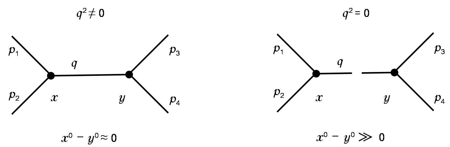
Figure 2: The schematic Feynman diagrams of the interaction of two particles in a massless theory.

shown in Fig. 2. When the time interval between vertexes $x$ and $y$ is very short, the magnitude of the energy-momentum vector for the propagator is non-zero and hence, the propagator is a virtual particle. However, when the time interval between these points is very long, the magnitude of the energy-momentum vector for the propagator is zero and hence, the propagator is a real particle. Therefore, for the first case, one needs to have one closed contour for real particles, while for the second case, two closed contours for real particles are required. Now consider another example in which five groups of particles interact with each other in a massless theory. If these five groups of particles move away from each other in such a way that the distances between those increase very much, then the propagators among those will become real particles (see, e.g., Fig. 3).

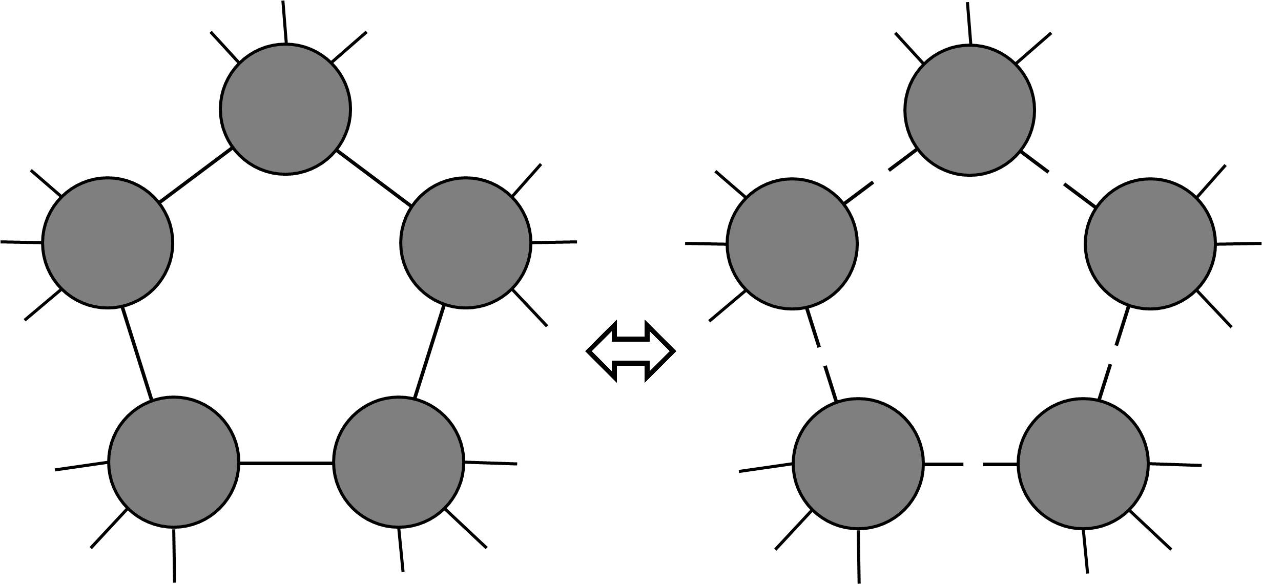
Figure 3: The schematic Feynman diagrams of the interaction of five groups of particles in a massless theory.

Each group of particles behaves like a composite particle and also interacts with other groups in a way that the outcome forms a closed contour of the momentum conservation. For example, see Fig. 4, wherein

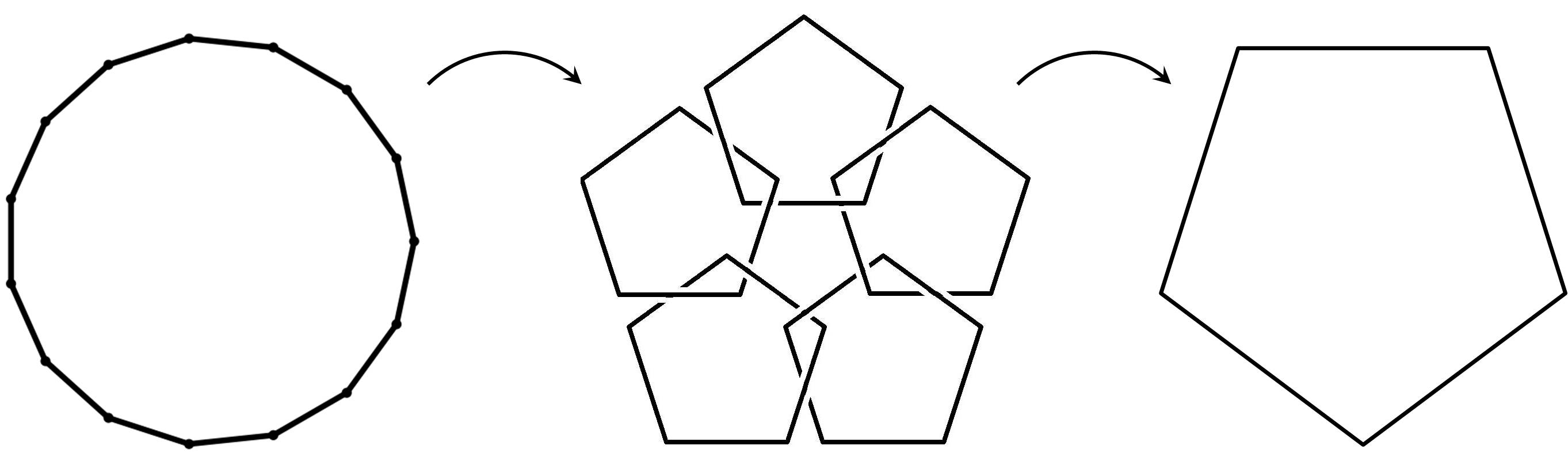
Figure 4: The closed contour of the momentum conservation of five groups of particles that move away from each other in such a way that the propagators among those become real particles, related to Fig. 3.

the reason for linking these five closed contours in this figure is that these five sets of particles are not independent of each other and interact with each other so that the result forms a closed contour of the momentum conservation. In the standard field theory, there is no significant physical difference between the left and right parts of Fig. 3. However, in the PT, geometrical difference of the left and right parts of Fig. 3 leads to different topology, and hence, physical properties.

Since links and knots have topological properties, we expect a correspondence between these topological properties, and in turn, the properties of the consisted structure of particles and interactions among those. For example, the carbon nanotubes, graphite and diamond are all made of carbon but have completely different properties. It is widely accepted that the difference in their properties is due to their different geometric structures in the placements of atoms of carbon. As an another example, let us mention the topological molecules Diudea , in which those atoms, that make up some of the molecules, may be the same but have completely different topological structures Forgan ; Shimokawa .

PT Description of Loop Level Scattering Amplitude:  From mathematical point of view, the result of the hidden particles method in describing loop corrections (mentioned in Refs. Elvang-2015 ; Arkani-Hamed-2011 ) is equivalent to what we have mentioned in the previous section. In fact, in the hidden particles method, two hidden particles are considered for each loop, and their momentum twisters are integrated in a certain way. On the other hand, in the previous section, instead of integrating on the momentum twisters of two hidden particles, the same number of Dirac delta functions have been removed and integrated on variables $y_{1}$ and $y_{2}$ in the same specific way.

Physically, from the PT point of view (also from the point of view of on-shell physics Elvang-2015 ; Arkani-Hamed-2011 ), a loop means the existence of a pair of entangled real particle-antiparticle whose energy-momentum vectors are opposite to each other. Thus, the existence of these pairs does not change the total energy-momentum, and therefore all possible values for their energy-momentum must be considered. This state is schematically as a state in which two points of the one-dimensional manifold touch each other Elvang-2015 (see, e.g., Fig. 5).

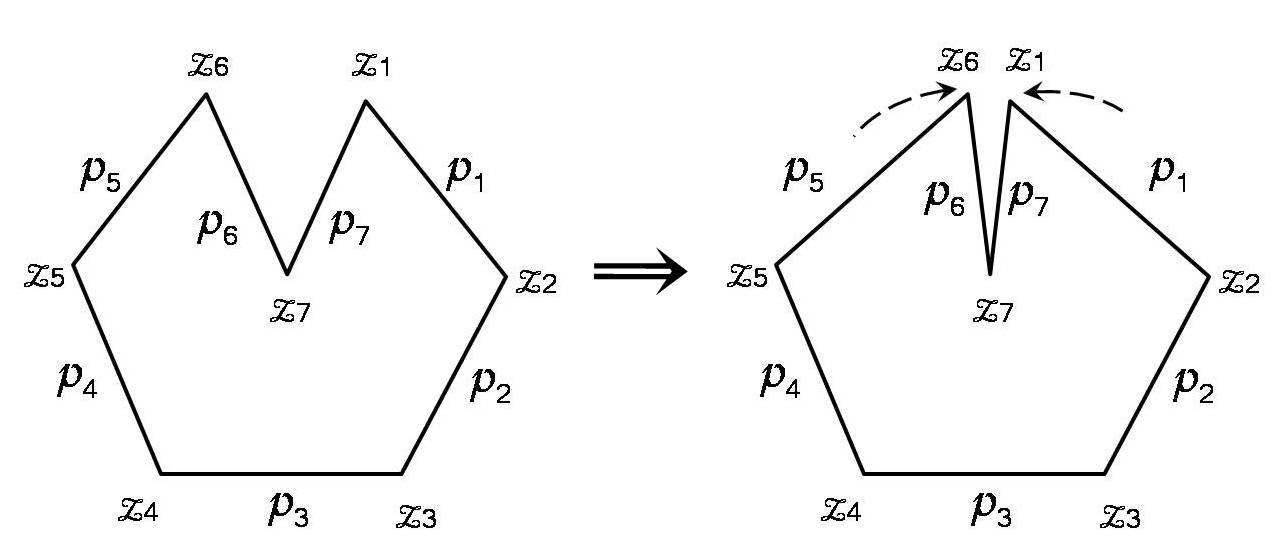
Figure 5: Forming a loop in the closed contour of the momentum conservation. After the points $z_{1}$ and $z_{6}$ touch each other, the energy-momentum vectors $p_{6}$ and $p_{7}$ will be equal and in opposite directions Elvang-2015 .

IX Conclusions

Inspired by the fact that geometric representation of the momentum conservation of particles participating in an interaction leads to the formation of a closed contour, we have introduced an integrable one-dimensional theory, i.e., the PT. This theory underlies some integrable models such as the KP-hierarchy and the amplituhedron. In this regard, we have defined the action and then the partition function of the PT. Afterward, we have shown that the fields of the PT are equivalent with their partition functions. Due to the quantization process, this issue means that the theory will not change after quantization. Therefore, this theory possesses a particular symmetry as a statistical symmetry. This symmetry implies that the theory, in small-scales, is statistically equivalent to large-scales (such a characteristic is what we have benefited in another work you-far ).

Also, by defining the S-matrix of the PT, we have indicated that the S-matrix has the Grassmannian structure. This Grassmannian corresponds to a chord diagram, which specifies the closed contour of the PT. Thereupon, by introducing and using a transformation (i.e., the hierarchy transformation), we have shown that the PT underlies some important kinds of integrable models in different dimensions such as the types of soliton models derived from the KP-hierarchy, two-dimensional models and the amplituhedron. Thus, we have represented that the S-matrix of the PT, after hierarchy transformation, is a solution of the KP-hierarchy.

Furthermore, we have indicated that the volume of phase-space of the one-dimensional manifold of the theory is equivalent with the Grassmannian integral. Indeed, contrary to Refs. Elvang-2015 ; Arkani-Hamed-2014 ; Arkani-Hamed-2016 ; Arkani-Hamed-2011 , without any use of supersymmetry, we have obtained a sort of general structure in comparison with the conventional Grassmannian integral and the resulted amplituhedron, which is closely related to the Yang-Mills scattering amplitudes in four dimensions. Accordingly, the common amplituhedron presented in the literature can be derived from the volume of phase-space of the proposed one-dimensional manifold as a special contour integration of the Grassmannian integral presented in this work, and being regarded as a particular choice of it. Indeed, the proposed theory is capable to express both the tree- and loop-levels amplituhedron (without employing hidden particles) in four dimensions in the twistor space. Finally, we have discussed the physical meaning and importance of the linked closed contour.

References

- (1) K. Kampf, J. Novotný and J. Trnka, “Tree-level amplitudes in the nonlinear sigma model”, J. High Energy Phys. 05 (2013), 032.
- (2) H. Elvang and Y. Huang, “Scattering Amplitudes in Gauge Theory and Gravity”, (Cambridge University Press, Cambridge, 2015).
- (3) J. Bijnens, K. Kampf and M. Sjö, “Higher-order tree-level amplitudes in the nonlinear sigma model”, J. High Energy Phys. 11 (2019), 074.
- (4) S.J. Parke and T.R. Taylor, “An amplitude for n-Gluon scattering”, Phys. Rev. Lett. 56 (1986), 2459.
- (5) M.L. Mangano and S.J. Parke, “Multi-parton amplitudes in gauge theories”, Phys. Rep. 200 (1991), 301.
- (6) R. Britto, F. Cachazo, B. Feng, and E. Witten, “Direct proof of the tree-level scattering amplitude recursion relation in Yang-Mills theory”, Phys. Rev. Lett. 94 (2005), 181602.
- (7) N. Arkani-Hamed and J. Trnka, “The amplituhedron”, J. High Energy Phys. 10 (2014), 030.
- (8) C. Callender, “Physics Meets Philosophy at the Planck Scale: Contemporary Theories in Quantum Gravity”, (Cambridge University Press, Cambridge, 2001).
- (9) M. Jimbo and T. Miwa, “Solitons and infinite dimensional Lie algebras”, Publ. RIMS, Kyoto Univ. 19 (1983), 943.
- (10) N. Ishibashi, “Soliton equations and free fermions on Riemann surfaces”, Mod. Phys. Lett. A 02 (1987), 119.
- (11) C. Vafa, “Operator formulation on Riemann surfaces”, Phys. Lett. B 190 (1987), 47.
- (12) E.P. Verlinde and H.L. Verlinde, “Chiral bosonization, determinants and the string partition function”, Nucl. Phys. B 288 (1987), 357.
- (13) J.M. Sullivan, “Curves of finite total curvature”, Disc. Diff. Geo. 38 (2008), 137.
- (14) P.R. Cromwell, “Knots and Links”, (Cambridge University Press, Cambridge, 2004).
- (15) S.A. Huggett and K.P. Tod, “An Introduction to Twistor Theory”, (Cambridge University Press, Cambridge, 1994).
- (16) T. Miwa, M. Jimbo and E. Date, “Solitons: Differential Equations, Symmetries and Infinite Dimensional Algebras”, (Cambridge University Press, Cambridge, 2000).
- (17) É. Cartan, “Les systèmes differentiels extérieure et leur applications géométriques”, (Hermann, Paris, 1945).
- (18) G.C. Wick, “Properties of Bethe-Salpeter wave functions”, Phys. Rev. 96 (1954), 1124.
- (19) M.E. Peskin and D. Schroeder, “An Introduction to Quantum Field Theory”, (Westview Press, New York, 1995).
- (20) G. Gentili and D.C. Struppa, “A new theory of regular functions of a quaternionic variable”, Adv. Math. 216 (2007), 279.
- (21) F.A. Berezin, “The Method of Second Quantization”, (Academic Press, London, 1966).
- (22) M. Yousefian and M. Farhoudi, “QED treatment of linear elastic waves in asymmetric environments”, Wa. Rand. Comp. Med. (2021), DOI:10.1080/17455030.2021.1938289.
- (23) M. Yousefian and M. Farhoudi, “Gravity as a ‘third’ quantization gauge theory with Minkowski metric, non-zero torsion and curvature”, arXiv: 2104.05768.
- (24) Y. Kodama, “KP Solitons and the Grassmannians Combinatorics and Geometry of Two-Dimensional Wave Patterns”, (Springer, Singapore, 2017).
- (25) Y. Kodama and L.K. Williams, “KP solitons, total positivity, and cluster algebras”, Proc. Nat. Acad. Sci. 108 (2011), 8984.
- (26) Y. Kodama and L.K. Williams, “KP solitons and total positivity for the Grassmannian”, Invent. Math. 198 (2014), 637.
- (27) S. Chakravarty and Y. Kodama, “Construction of KP solitons from wave patterns”, J. Phys. A 47 (2014), 025201.
- (28) N. Arkani-Hamed, et al. “Grassmannian Geometry of Scattering Amplitudes”, (Cambridge University Press, Cambridge, 2016).
- (29) N. Arkani-Hamed, H. Thomas and J. Trnka, “Unwinding the amplituhedron in binary”, J. High Energy Phys. 01 (2018), 016.
- (30) N. Arkani-Hamed, Y. Bai and T. Lam, “Positive geometries and canonical forms”, J. High Energy Phys. 11 (2017), 039.
- (31) R. Kojima and C. Langer, “Sign flip triangulations of the amplituhedron”, J. High Energy Phys. 05 (2020), 121.
- (32) N. Arkani-Hamed, F. Cachazo and C. Cheung, “The Grassmannian origin of dual superconformal invariance”, J. High Energy Phys. 03 (2010), 036.
- (33) N. Arkani-Hamed, J. Bourjaily, F. Cachazo, S. Caron-Huot and J. Trnka, “The all-loop integrand for scattering amplitudes in planar =4 SYM”, J. High Energy Phys. 01 (2011), 041.
- (34) Z. Bern, J.J. Carrasco, T. Dennen, Y.-t. Huang and H. Ita, “Generalized unitarity and six-dimensional helicity”, Phys. Rev. D 83 (2011), 085022.
- (35) N. Craig, H. Elvang, M. Kiermaier and T.R. Slatyer, “Massive amplitudes on the Coulomb branch of 4 SYM”, J. High Energy Phys. 12 (2011), 097.
- (36) M.V. Diudea, I. Gutman and J. Lorentz, “Molecular Topology”, (Nova Science Publishers, New York, 2001).
- (37) R.S. Forgan, J.P. Sauvage and J.F. Stoddart, “Chemical topology: Complex molecular knots, links, and entanglements”, Chem. Rev. 111 (2011), 5434.
- (38) K. Shimokawa, K. Ishihara and Y. Tezuka, “Topology of Polymers”, (Springer, Tokyo, 2019).