Template-Instance Loss for Offline Handwritten Chinese Character Recognition

Abstract

The long-standing challenges for offline handwritten Chinese character recognition (HCCR) are twofold: Chinese characters can be very diverse and complicated while similarly looking, and cursive handwriting (due to increased writing speed and infrequent pen lifting) makes strokes and even characters connected together in a flowing manner. In this paper, we propose the template and instance loss functions for the relevant machine learning tasks in offline handwritten Chinese character recognition. First, the character template is designed to deal with the intrinsic similarities among Chinese characters. Second, the instance loss can reduce category variance according to classification difficulty, giving a large penalty to the outlier instance of handwritten Chinese character. Trained with the new loss functions using our deep network architecture HCCR14Layer model consisting of simple layers, our extensive experiments show that it yields state-of-the-art performance and beyond for offline HCCR.

I Introduction

HCCR has been extensively studied for over 40 years. To deal with the challenge of large number of character classes, numerous approaches have been proposed to improve recognition accuracy, though the recognition results were still unsatisfactory. In hindsight, the recognition task is extremely challenging due to two reasons: 1) many Chinese characters have intrinsic similarities in structure; 2) great diversity of handwriting style makes the recognition problem more difficult. Traditional handcrafted features are incapable of representing well the inherent high complexity of Chinese characters. We believe that the limit has reached for handcrafted features for handwritten Chinese characters recognition, but unfortunately the pertinent recognition accuracy is still far from human performance.

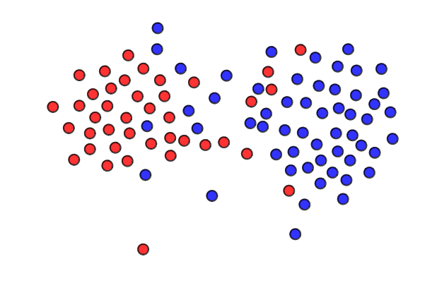
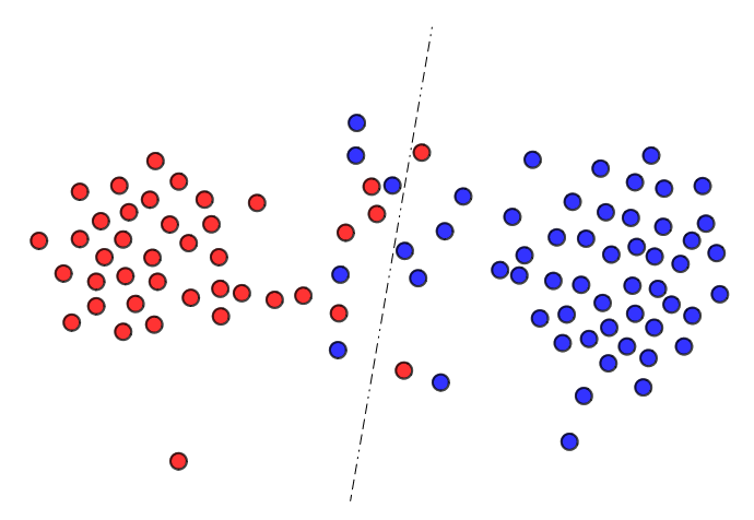
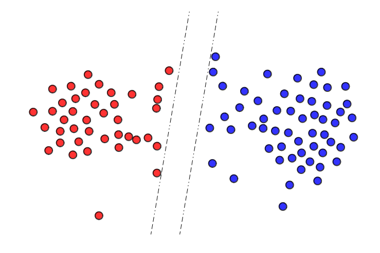
(a) Original	(b) Template	(c) Template+instance

Figure 1: Illustration of template-instance loss. The template loss works on category level, and the instance loss affects misclassified samples.

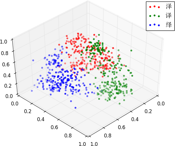
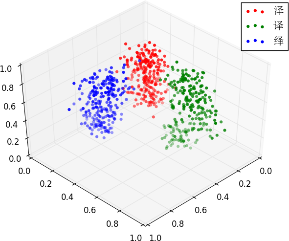
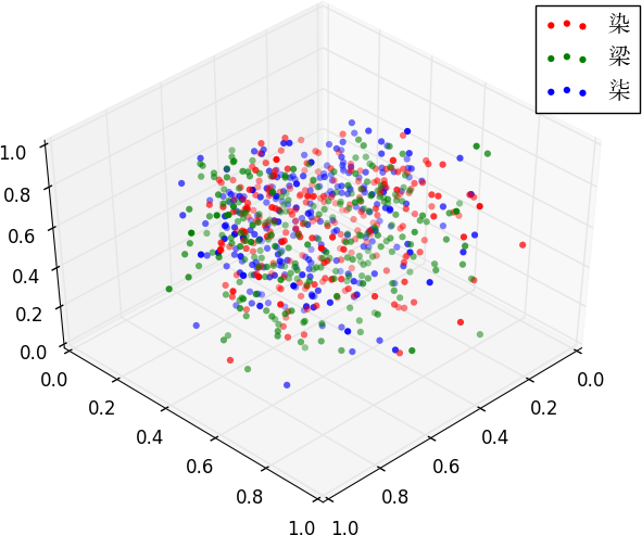
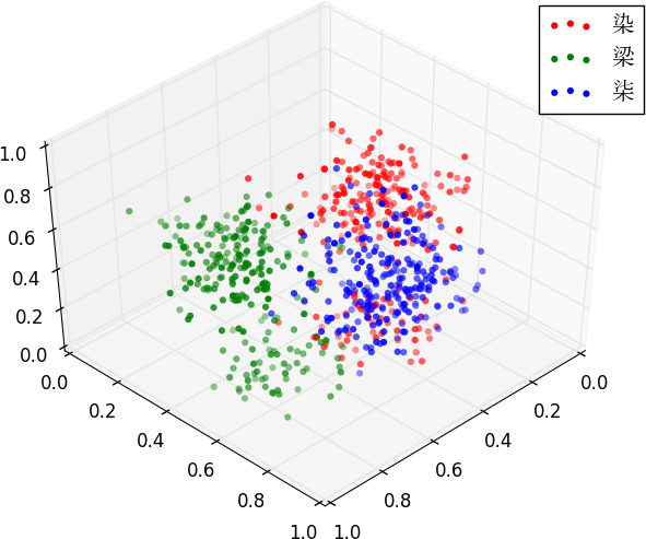
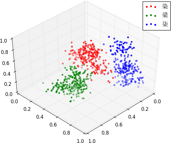
(a) Original image	(b) Softmax	(c) Template loss

Figure 2: Comparison of original image, softmax loss and our template loss. Characters with similar structure can be clearly separated with our proposed loss function.

The technical advent of computational power in recent years has fueled the development of deep convolution neural networks (CNNs) which have surpassed traditional machine learning in various problem domains. In particular, Ciresan et al. [1] first proposed the multi-column deep neural network (MCDNN), which was composed of several CNNs, to address the HCCR problem. Since then, the relevant state-of-the-art performance has been progressively improved. In the mean time, CNN is also evolving as well, with numerous new and effective network architectures and loss functions proposed to solve various problems.

To improve classification performance on large scale categories dataset, researchers have proposed various loss functions which have achieved impressive results in face recognition [10, 9, 15, 16, 2]. In summary, these loss functions are different variants of softmax loss. The intuition is to add a margin on the decision boundary to increase the distance between different categories. Nonetheless all previous methods expand a fixed decision margin in various manifolds. However, the Chinese character system is highly complicated. We observe two main difficulties: (1) many characters are similar, or partially similar in structure. Some print characters hold the common skeleton, e.g., the difference of three examples in the first row of Figure 3 consist of one stroke only. On the other hand, most characters are composed of a number of radicals. Different characters may contain the same radical, and most of characters are partially similar, e.g., the second row of Figure 3; (2) Handwritten strokes can easily lead to recognition confusion. Comparing to printed text, handwriting is usually distorted. Moreover, cursive handwriting produces stroke connections which can obscure the original structure of the character. For example, in Figure 4, the vertical stroke makes it much more difficult in distinguishing the two handwritten characters.

To handle the first challenge, we use print characters as templates of handwritten text. From character templates, we propose a measurement prior for template similarity. First we choose a set of image features to produce a measurement of print character similarity individually, followed by integrating them through dimension reduction to generate the final distance. Then, we set a prior margin between each class based on the estimated distance. We choose 8 kinds of standard Chinese font as templates and compute a mean feature over them. The final distance can sufficiently measure the similarity between two given templates.

To address the second challenge, we introduce an instance level loss function. Each handwritten character can be treated as an instance of template, with stroke variance introduced. we observe that the lack of clarity in handwriting introduces a number of difficult examples, which are far from class center. However there are still a lot of clearly written samples that can be easily distinguished by the classifier. In other words, there exists an imbalance between hard and easy samples. To increase the attention paid to the outliers, we propose our adaptive margin to dynamically fit the training loss to bias hard samples. The intuition is to add a moderating factor that is controlled by the estimated probability for the ground-truth class. Specifically, if the sample is far from class center, it will be given a large margin to other classes, thus increasing its contribution in the final loss function, and vice versa. With this re-balancing moderation, badly written characters will be given more attention. Outliers will be contracted to the class center, reducing category variance. We will demonstrate the effectiveness of our adaptive margin in the experiment section.

In summary, in this paper we propose two new types of loss function to deal with HCCR difficulties. Our contribution includes: 1) a new prior margin to handle character template similarity; 2) a new adaptive margin to reduce category instance variance; 3) an elaborate network architecture to accomplish HCCR task. Extensive experiments demonstrate that our networks are able to achieve state-of-the-art performance.

Figure 3: Ambiguous characters. Characters in the first row only differ in one stroke while those in the second row share the exactly same radical.

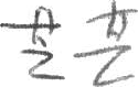
(a) Print	(b) Handwritten

Figure 4: Comparison of print and handwritten text. Stroke connection in handwritten text may cause confusion in recognition.

II Related Work

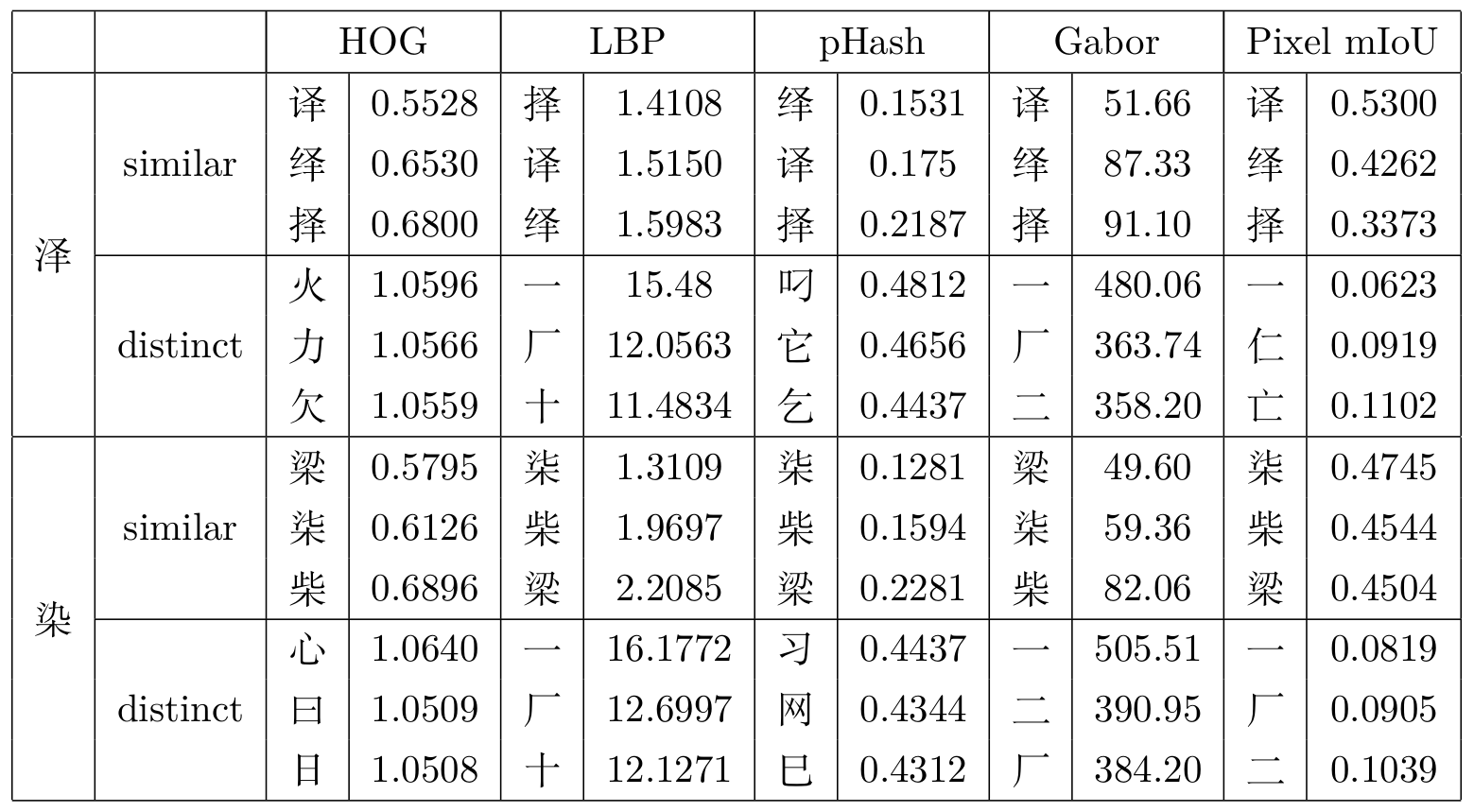
Figure 5: Estimated distance of templates.

II-A Offline HCCR

Handwritten Chinese Character Recognition (HCCR) has been intensively studied since 1980s. Traditional HCCR methods have three procedures: pre-processing, hand-crafted feature extraction, and classification. Recently, significant progress has been achieved by leveraging the great success of deep convolutional neural networks (CNN) in various domains. Multi-column deep neural network (MCDNN) [1] was the first successful application of CNN to offline HCCR, with the best performance of single network achieving an accuracy of 94.47%, which was improved to 95.78% by ensembling 8 networks. Since then, more researchers have shifted their attention from traditional methods to deep CNN models for HCCR. In the offline HCCR competition held by ICDAR in 2013, Yin et al. [21] won the first place with the recognition rate of 94.77%. A year later, the accuracy was improved to 96.06% by using a voting strategy on four ATR-CNNs [19]. In 2015, Zhong et al. [23] combined traditional feature extraction methods with GoogLeNet, and obtained an accuracy of 96.35%, 96.64%, and 96.74% with single, four and ten ensemble models, respectively. With these results, accuracy reported in  [23] became the first to surpass human performance. In 2017, Zhong et al. [22] further improved the accuracy to 96.95% by the combination of traditional DirectMaps and CNNs. Xiao et al. [20] designed a nine-layer CNN model with network pruning and achieved an accuracy of 97.09%, with only 1/18 size of its original size.

II-B Loss Function

Loss function is analogous to a ruler for deep learning, which is used to measure a given model and guide the training. Therefore, the design of loss function is as important as the model structure design. Loss function is used to evaluate the relationship between the predicted value and the ground truth value. Euclidean loss, hinge loss, softmax loss, etc. are widely used in deep CNN models. Contrastive loss [3] increases the inter-class and reduces the intra-class variance to get better deep features. Similar to contrastive loss [3], triplet loss [13] introduces triple sample pairs {x: input, x1: positive, x2: negative} to increase Euclidean margin for better feature embedding. Since contrastive loss and triplet loss need to use pair label information, both of them require a careful design of pair selection procedure. Center loss [18] was proposed to learn centers for deep features of each sample. The distribution of these deep features is uniform within the same class, which helps to reduce intra-class variance. Large margin softmax (L-softmax) [10] adds cosine distance constrain to each identity, with the aim of enhancing the inter-class compactness and inter-class separability. Deep CNN models with angular softmax (A-softmax) [9] can learn more discriminative features by normalizing the weights based on L-softmax.

Large margin cosine loss [16], Additive Margin Softmax (AM-softmax) [15] and Additive angular margin loss [2] all transform the original softmax loss function into a cosine loss style by normalizing the deep features and the weights. The normalization eliminates the variance in radial direction (compared to L-Softmax) and a cosine based margin is introduced. This margin was used to further maximize the decision boundary of the learned features in the angular space. Wan [14] proposed Large-margin Gaussian Mixture (LGM) loss, assuming that deep feature satisfied Gaussian mixture distribution and a certain classification margin at the same time. Lin [7] proposed focal loss to make the model more focused on difficult samples by reducing the weight of the easily classified samples.

III Template-Instance Loss Functions

We propose two novel loss function, namely template and instance loss. For the $i^{th}$ category, we derive our loss from additive margin [15] due to its simplicity:

$$L_{i}=-\log\frac{e^{s(\cos\theta_{y_{i}}-m)}}{e^{s(\cos\theta_{y_{i}}-m)}+\sum_{j=1,j\neq y_{i}}^{n}e^{s\cos\theta_{j}}}$$ (1)

where $y_{i}$ is the ground-truth label, $s$ is a scale factor and $m$ is the embedded margin.

III-A Template Loss

There exists intrinsic similarity among different templates of Chinese characters due to the unique structure of the Chinese character system. The Chinese dictionary provides isomorphic characters as reference. Typically these look-like characters are searched by humans, and the relevant similarity cannot be quantified. We seek to compare all commonly used characters templates to calculate an template affinity matrix as the prior margin.

There is no existing rule to define Chinese characters similarity. To quantify how two templates look like, we assemble a number of classical vision features as feature pool, including pixel-wise mIoU, pHash, SIFT, Hog and Gabor feature. To sidestep the irregularity of handwriting, we utilize gray-scale images of multiple standard fonts, such as SimSun, SimHei, FangSong, KaiTi and so on, as templates and compute features upon them. The average template feature distance is computed as the mean over all the fonts. See Figure 5 for demonstration.

However, different features are unrelated and exist in different spaces. We need to integrate them to produce our template affinity representation. Hence a proper normalization is needed. A naive solution is to linearly rescale each individual feature similarity to the range [0,1]. However some distance has unlimited upper bound which leads to scale imbalance. Instead, we perform a dimension reduction to generalized normalized score like [11].

Given $K$ features and $N$ templates, we define directional similarity $N\times K$ matrix $\mathbf{S}^{i}$ , which encodes the similarity between template $i$ and others over all features. Element $s^{i}_{k,j}$ represents similarity of feature $k$ between template $i$ and $j$. Since $\mathbf{S}^{i}$ is not symmetric, we compute its SVD decomposition

$$\mathbf{S}^{i}=\mathbf{U}^{i}\mathbf{S}^{i}{\mathbf{V}^{i}}^{T}$$ (2)

and the normalized ($N$ dimensions ) similarity vector $\mathbf{\hat{h}}^{i}$ is defined as the column of $\mathbf{V}^{i}$ corresponding to the maximum singular value. Similar to eigenvector, the elements of principal column of $\mathbf{V}^{i}$ are a measures of centrality, and are proportional to the amount of time that an infinite-length random walk on $\mathbf{S}^{i}$ will spend [11] to measure the distance of two templates. We stack the $N$ normalized vector for all templates to obtain a matrix $\mathbf{H}$ and the affinity matrix is expressed as

$$\mathbf{A}=\frac{\mathbf{H}+\mathbf{H^{T}}}{2}$$ (3)

which will be rescaled to normalize the diagonal elements. $a_{ij}$ indicate the similarity of two templates.

With the affinity matrix we define our prior margin between template $i$ and $j$ as the softmax probability:

$$m^{P}(i,j)=\left\{\begin{aligned} &\frac{e^{a_{ij}}}{\sum_{j}e^{a_{ij}}},&j\neq i\\ &0,&j=i\end{aligned}\right.$$ (4)

where $a_{ij}$ is the $(i,j)$ element of $\mathbf{A}$. We embed the margin into  Equation 1:

$$L_{i}=-\log\frac{e^{z_{y_{i}}}}{\sum_{j=1}^{n}e^{z_{j}+\beta m^{P}_{ij}}}$$ (5)

where $\beta$ is a scaling factor. After integrating the prior margin, highly similar template pair needs a larger decision boundary to be distinguished. Note that the prior margin is fixed for the whole category. Template loss works on class level, affecting the class center and scale. As for the hard samples or outliers, we need another loss function to deal with individually.

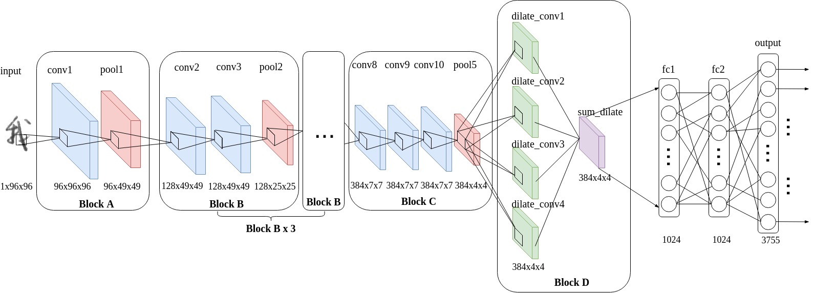
Figure 6: Network architecture.

III-B Adaptive Margin

Recent methods [10, 9, 15, 16, 2] all expand a fixed decision margin in various manifolds. These margins constrain trained features to be compact around class center, including both hard and easy samples. However, according to [7], in the detection process there exist a large number of background samples which are easy to classify. These easy samples can overwhelm hard positive ones and dominate the final loss. Similar situations occur for Chinese characters, because well-written instance could be easily distinguished, while badly-written ones are hard to be recognized. Since common radicals occur among distinct Chinese characters, stroke confusion raises classification difficulty. Therefore, it is of significant importance to adaptively impose the margin according to classification difficulty of each instance. We propose instance loss, which is achieved by adaptive margin based on the softmax loss. To evaluate the difficulty of input instance, we use the estimated probability for the ground-truth label $y_{i}$:

$$p_{i}=\frac{e^{z_{y_{i}}}}{\sum_{j}e^{z_{j}+\beta m^{P}_{ij}}}$$ (6)

Then we define our adaptive margin as

$$m^{A}_{i}=\alpha(1-p_{i})^{\gamma}$$ (7)

where $\alpha$ is the upper-bound of margin. Our margin has two desirable properties: (1) When an instance is far from class center and misclassified, $p$ should be small and the margin is maximized to its upper-bound $\alpha$, thus leading to larger penalty for the misclassification. As $p\to 1$, the margin goes to $0$ and the loss for well-classified samples will be close to the original softmax loss; (2) The parameter $\gamma$ smoothly adjusts the margin scale between easy and hard samples. When $\gamma=0$, $m$ is the same as additive margin, and as $\gamma$ increased the effect of margin adaptability is also enhanced. Since $m_{i}^{A}$ depends on $p_{i}$, which is the estimated probability of individual sample, the adaptive margin works on instance level, increasing the punishment of difficult samples or outliers.

Putting Equations 6 and 7 into 1 we get:

$$L_{i} =-\log\frac{e^{s(\cos\theta_{y_{i}}-m^{A}_{i})}}{e^{s(\cos\theta_{y_{i}}-m^{A}_{i})}+\sum_{j=1,j\neq y_{i}}^{n}e^{s\cos\theta_{j}+\beta m^{P}_{ij}}}$$

$$=-\log\frac{e^{-sm^{A}_{i}}}{\frac{\sum_{j}^{n}e^{s\cos\theta_{j}+\beta m^{P}_{ij}}}{e^{s\cos\theta_{y_{i}}}}+e^{-sm^{A}_{i}}-1}$$

$$=-\log\frac{e^{-sm^{A}_{i}}}{\frac{1}{p}+e^{-sm^{A}_{i}}-1}$$

$$=-\log\frac{1}{(\frac{1}{p_{i}}-1)e^{s\alpha(1-p_{i})^{\gamma}}+1}$$ (8)

In practice the $\alpha$ is not a fixed parameter. It increases with iteration number rising in a sigmoid style, i.e., at the beginning of training the loss is approximately the same with softmax. With the training proceeding, the margin influence will gradually increase, thus weakening contribution of easy samples. We will further discuss the setting of $\alpha$ in experiment section.

IV HCCR Networks

The architecture of our designed network is shown in Figure 6. The input image is resized to $96\times 96$ which slightly increases performance. Except for converting the RGB image into gray format and subtracting the mean gray value, we do not perform other preprocessing. The resized images are then passed through a stack of blocks and fully connected layers.

In this paper, we design four kinds of blocks, namely, Block A to Block D. Block A consists of one Conv-BN-PReLU module, followed by a max pooling layer over a $3\times 3$ window with stride of 2 and one pixel padding. The only difference between Block A, Block B, and Block C is the number of Conv-PReLU-BN modules. In Block B and Block C, the number of Conv-BN-PReLU modules is two and three, respectively. Convolutional kernels in Block A to C are $3\times 3$, with padding size of 1 and stride of 1. Block D is a hybrid dilated convolution (HDC) module [17], which includes a multi-dilated convolution layer and a pixelwise summation of the multi-dilated convolutional feature maps. After dilation, the dilated convolutional kernel size is changed from $k\times k$ into $r\times\left(k-1\right)+1$, where $k\times k$ is the original convolutional kernel size, and $r$ is the dilation rate. In order to retain the size for summation, the padding pixels are computed in accordance with the dilation rate of the kernel. In this paper, after the last pooling layer, the size of feature maps is $4\times 4$. The kernel sizes for the 4-channels dilation convolutional layers are all $3\times 3$, with dilation rates and padding pixels ranging from 1 to 4. These multi-dilated convolutional feature maps are summed up before sending into the subsequence fully connected fc1, fc2 and output layers. Fc1 and fc2 contains 1024 neurons, equipped with batch normalization (BN) [5] and parametric rectified linear unit (PReLU) [4]. Features in fc2 layer are applied L2 normalization before sent into the last output layer, which has 3755 neurons to carry out the final Chinese character recognition task.

The overall architecture is illustrated in 6, which contains 10 Conv-BN-PReLU modules, 5 pooling layers, 1 multi-dilated convolutional, and 3 fully connected layers. As a result, our network architecture is designed as a 14-layer network (only accounting for the convolutional and fully connected layers). We refer to this network as HCCR14layer.

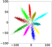
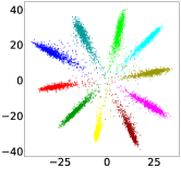
(a)	(b)	(c)	(d)
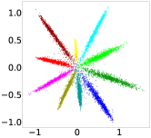
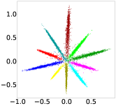
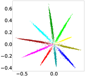
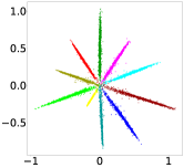
(e)	(f)	(g)	(h)

Figure 7: Visualization of two-dimensional feature embeddings on MNIST training set. First row: (a) Softmax loss. (b) Large-margin softmax loss [10]. (c) Additive margin loss [15]. (d) Adaptive margin loss. Second row: (e-h) Adaptive margin with $\alpha=0.1,0.2,0.3,0.4$. Margin effect expands with $\alpha$ increasing.

The main difference between our proposed HCCR14layer and other previous models for offline HCCR is that HCCR14layer involves PReLU, BN, and HDC layer. In our proposed network, all convolutional layers in Block A, B, C, and two fully-connected layers (fc1 and fc2) are followed by BN and PReLU layer. The BN layer was proposed by Ioffe et al. [5], which can not only efficiently speed up network convergence, but also effectively avoid the problem of vanishing gradients during training. The PReLU [4], with a parametric constrain based on ReLU [12], was shown to be able to handle vanishing and exploding gradient. Since PReLU [4] contains only a few parameters, the network can still easily converge to the optimal state, while risking a bit to overfitting.

The template and instance loss functions are combined as the final loss. Our proposed loss will rebalance the contribution of training samples according to template similarity and instance difficulty, improving model performance. Although the proposed HCCR14Layer model employs quite simple layers, it yields state-of-the-art performance for offline HCCR by cooperating with our novel template-instance loss.

V Experiments

We conducted extensive experiments to verify the effectiveness of our novel loss. We also present experimental results of our HCCR networks and perform comparison with state-of-the-art methods.

We used the data obtained from offline CASIA-HWDB1.0 (HWDB1.0) and CASIA-HWDB1.1 (HWDB1.1) [8] for training, and ICDAR-2013 [21] competition data for testing, which were provided by the Institute of Automation of the Chinese Academy of Sciences. The detailed information about these datasets are listed in Table III. The training set contains 2,678,424 samples written by 720 people, and 3,755 characters in the GB2312-80 level-1 set. The testing dataset contains 224,419 samples written by another 60 people. Before training, we merged HWDB1.0 and HWDB1.1 to get HWDB1.0+1.1 with respect to HWDB1.1’s class labels. We have also made sure that the merged dataset HWDB1.0+1.1 and ICDAR-2013 have the same class label.

V-A Adaptive and Prior Margin

$\alpha_{max}$	0 (softmax)	0.01	0.05	0.1	0.2
Accuracy (%)	94.49	95.32	95.59	95.75	95.66

TABLE I: Performance of instance loss with different setting. Note that $\alpha_{max}=0$ is original softmax

In Figure 7 we perform a toy experiment to better visualize the margin effect on features. We extract features on MNIST dataset using other losses and our proposed adaptive margin. In this experiment we fix $\alpha$ for simplicity. We show various results with different $\alpha$s for comparison. As shown in the figure, the first row displays the comparison of the original softmax, large margin softmax (LM), additive margin (AM) and our adaptive margin (AD). We can observe that our adaptive margin shows strong margin effect. As $\alpha$ increases, the angular margin between classes are amplified, as shown in the second row.

Layers	A	B	C
Bloak A	$\left[\begin{tabular}[]{@{}c@{}}Conv-BN-PReLU\\ Pool\end{tabular}\right]$ $\times 3$	$\left[\begin{tabular}[]{@{}c@{}}Conv-BN-PReLU\\ Pool\end{tabular}\right]$ $\times 1$	$\left[\begin{tabular}[]{@{}c@{}}Conv-BN-PReLU\\ Pool\end{tabular}\right]$ $\times 1$
Bloak B	$\left[\begin{tabular}[]{@{}c@{}}Conv-BN-PReLU\\ Conv-BN-PReLU\\ Pool\end{tabular}\right]$ $\times 2$	$\left[\begin{tabular}[]{@{}c@{}}Conv-BN-PReLU\\ Conv-BN-PReLU\\ Pool\end{tabular}\right]$ $\times 3$	$\left[\begin{tabular}[]{@{}c@{}}Conv-BN-PReLU\\ Conv-BN-PReLU\\ Pool\end{tabular}\right]$ $\times 3$
Bloak C	/	$\left[\begin{tabular}[]{@{}c@{}}Conv-BN-PReLU\\ Conv-BN-PReLU\\ Conv-BN-PReLU\\ Pool\end{tabular}\right]$ $\times 1$	$\left[\begin{tabular}[]{@{}c@{}}Conv-BN-PReLU\\ Conv-BN-PReLU\\ Conv-BN-PReLU\\ Pool\end{tabular}\right]$ $\times 1$
Bloak D	HDC
Fully Connected Layer	1024FC-BN-PReLU	1024FC-BN-PReLU	1024FC-BN-PReLU 1024FC-BN-PReLU
Classification Layer	3755FC

TABLE II: Configurations for HCCR (shown in columns). The dropout layer is not shown for different dropout ratios.

Dataset	$\#$samples	$\#$class	$\#$writers
HWDB1.0	1,556,675	3,740	420
HWDB1.1	1,121,749	3,755	300
ICDAR-2013	224,419	3,755	60

TABLE III: Statistics of offline isolated character datasets

Feature	HOG	LBP	pHash	Gabor	Pixel. mIoU
Accu (%)	87.61	79.63	81.66	82.97	85.47

TABLE IV: Verification of human perception and feature similarity.

We also demonstrate the performance boost of HCCR by adaptive margin. In this experiment we use our HCCR 12 layers as base network. Original softmax and the proposed adaptive margin are applied to compare the results, and template loss is not integrated. For the training and testing data, we choose CASIA HWDB1.1, which includes 897,758 training and 223,991 testing samples. Input images are resized to $96\times 96$ to increase performance, similarly done in [20].

Method	Input	Image Size	Accuracy (%)
HCCR-Gabor-GoogLeNet [23]	Gabor Feature Maps + Gray Image	$9\times 120\times 120$	96.35
DirectMap+ConvNet [22]	Direct Feature Maps	$8\times 32\times 32$	96.95
HCCR-CNN9Layer+Skeleton [17]	Gray Image + Skeleton	$1\times 96\times 96$	96.90
HCCR-CNN9Layer[20]	Gray Image	$1\times 96\times 96$	97.09
HCCR-WAP [6]	Gray Image	$1\times 64\times 64$	96.91
HCCR14Layer+softmax	Gray Image	$1\times 96\times 96$	97.20
HCCR14Layer+additive margin loss	Gray Image	$1\times 96\times 96$	97.31
HCCR14Layer+template-instance loss	Gray Image	$1\times 96\times 96$	97.45

TABLE V: Recognition accuracies on ICDAR-2013 dataset of different network configurations. All models are trained on HWDB1.0+HWDB1.1.

HCCR config. (Table II)	Accuracy (%)
A, without fc1 norm	96.80
A, fc1 norm	96.84
B, without fc1 norm	97.37
B, fc1 norm	97.40
C, without fc2 norm	97.40
C, fc2 norm	97.45
C(all conv), without fc2 norm	97.35
C(all conv), fc2 norm	97.38

TABLE VI: Recognition accuracies on ICDAR-2013 dataset of different network configurations. All models are trained on HWDB1.0+HWDB1.1.

The factor $\alpha$ in Equation 7 is a tuning parameter to control the strength of margin. Due to the adaptive mechanism, the difficult samples, which is estimated by the softmax probability, will be given a large margin to produce a larger contribution to the total loss. However, at the beginning of training, if we train from scratch the model cannot classify well training samples and produce inaccurate estimated probabilities. Thus the margin contribution will be amplified, leading to either not converging, or fast converging to a local optimization. To avoid this we moderate $\alpha$ by a sigmoid function:

$$\alpha=\frac{\alpha_{max}}{1+e^{-\rho(\frac{iter}{max\_iter}-0.5)}}$$ (9)

At the training starts, $\mathit{iter}=1,\alpha\to 0$. At the end, $\alpha\to\alpha_{max}$. When $\alpha=0$, the loss is equivalent to the softmax loss. Thus the training loss is smoothly decreasing in the beginning phase. As the training is progressing, increasing $\alpha$ imposes extra training difficult, resulting in the loss bouncing back. In our experiments $\rho$ is set to be 10. We also compare results with different $\alpha_{max}$ settings. As tabulated in Table I, with adaptive margin the accuracy surpass original softmax. Among all settings $\alpha=0.1$ outperforms others. Therefore in our following experiments $\alpha$ is set to be 0.1.

On the other hand, to prove the representative ability of the selected features, we conduct experiments to verify consistency between human perception and template feature similarity. Three persons were asked to randomly pick three templates (A,B,C) from the alphabet. Each person give a judgment if template A is more similar to B, or C. If three people have disagreement, we accept the majority opinion. Then we compute the similarity of (A,B) and (A,C) to compare to human opinion. The test is repeated 500 times. The accuracy of every feature are listed in Table IV. We can see that selected features are basically consistent with human perception, among them HOG and pixel mIoU perform better.

V-B HCCR14Layer

We trained our proposed HCCR14Layer model (Figure 6) using mini-batch gradient descent with batch size of 128 and momentum of 0.9 for training. The base learning rate was set to 0.1, and was reduced to 1/10 every 70,000 iterations. Training was completed after 360,000 iterations. Finally, the curve tended to reach a steady state with an accuracy of 97.45% on the testing set.

We also evaluated other network configurations for HCCR in this paper, and all configurations follow the generic design presented in Section III-A. We report the performance of different configurations (outlined in Table II) on the testing dataset in Table VI. From the table we can see that deeper network can get better results, and feature normalization can slightly increase performance. In Table VI, we also replace the max pooling layer in Block A, B, and C into convolutional layer with kernel size $3\times 3$ and stride of 2. Compared with the last row in Table VI, we find that our proposed HCCR14Layer (configuration C in Table II) achieves better recognition accuracy. The main reason is that pooling layer in HCCR14Layer block modules can not only simplify the complexity of network when computing, but also extract the representative features during feature compression.

In Table V, we compared our proposed network and loss with the other available methods and losses. It is noteworthy that our proposed approach outperforms the other HCCR recognition models, achieving a state-of-the-art recognition rate of 97.45%.

VI Conclusion

Handwritten Chinese character recognition has been a long-standing problem until recent development of deep CNNs which produced revolutionary improvement to recognition accuracies. In this paper we propose template-instance loss function to address HCCR: 1) a new prior margin to handle character template similarity; and 2) a new adaptive margin to rebalance easy and difficult instance. We propose and implement a carefully designed network architecture to accomplish HCCR task using our new loss functions. Extensive experiments demonstrate that our network has pushed the frontier of recognition accuracy beyond the existing state-of-the-art methods. In the future, we plan to apply our template-instance loss on other classification tasks such as object detection and face recognition. We believe that the two-level type loss function should generally boost classification performance on large scale dataset.

References

- [1] D. Cireşan and U. Meier. Multi-column deep neural networks for offline handwritten chinese character classification. In Neural Networks (IJCNN), 2015 International Joint Conference on, pages 1–6. IEEE, 2015.
- [2] J. Deng, J. Guo, and S. Zafeiriou. Arcface: Additive angular margin loss for deep face recognition. arXiv preprint arXiv:1801.07698, 2018.
- [3] R. Hadsell, S. Chopra, and Y. LeCun. Dimensionality reduction by learning an invariant mapping. In IEEE Computer Society Conference on Computer Vision and Pattern Recognition (CVPR), pages 1735–1742. IEEE, 2006.
- [4] K. He, X. Zhang, S. Ren, and J. Sun. Delving deep into rectifiers: Surpassing human-level performance on imagenet classification. In Proceedings of the IEEE international conference on computer vision, pages 1026–1034, 2015.
- [5] S. Ioffe and C. Szegedy. Batch normalization: Accelerating deep network training by reducing internal covariate shift. In Proceedings of International Conference on Machine Learning (ICML), pages 448–456, 2015.
- [6] Z. Li, N. Teng, M. Jin, and H. Lu. Building efficient cnn architecture for offline handwritten chinese character recognition. arXiv preprint arXiv:1804.01259, 2018.
- [7] T.-Y. Lin, P. Goyal, R. Girshick, K. He, and P. Dollár. Focal loss for dense object detection. arXiv preprint arXiv:1708.02002, 2017.
- [8] C.-L. Liu, F. Yin, D.-H. Wang, and Q.-F. Wang. Casia online and offline chinese handwriting databases. In Document Analysis and Recognition (ICDAR), 2011 International Conference on, pages 37–41. IEEE, 2011.
- [9] W. Liu, Y. Wen, Z. Yu, M. Li, B. Raj, and L. Song. Sphereface: Deep hypersphere embedding for face recognition. In The IEEE Conference on Computer Vision and Pattern Recognition (CVPR), volume 1, page 1, 2017.
- [10] W. Liu, Y. Wen, Z. Yu, and M. Yang. Large-margin softmax loss for convolutional neural networks. In ICML, pages 507–516, 2016.
- [11] N. Masuda, M. A. Porter, and R. Lambiotte. Random walks and diffusion on networks. Physics Reports, 2017.
- [12] V. Nair and G. E. Hinton. Rectified linear units improve restricted boltzmann machines. In Proceedings of the 27th international conference on machine learning (ICML-10), pages 807–814, 2010.
- [13] F. Schroff, D. Kalenichenko, and J. Philbin. Facenet: A unified embedding for face recognition and clustering. In Proceedings of the IEEE conference on computer vision and pattern recognition, pages 815–823, 2015.
- [14] W. Wan, Y. Zhong, T. Li, and J. Chen. Rethinking feature distribution for loss functions in image classification. In IEEE Conference on Computer Vision and Pattern Recognition (CVPR), 2018.
- [15] F. Wang, J. Cheng, W. Liu, and H. Liu. Additive margin softmax for face verification. IEEE Signal Processing Letters, 25(7):926–930, 2018.
- [16] H. Wang, Y. Wang, Z. Zhou, X. Ji, Z. Li, D. Gong, J. Zhou, and W. Liu. Cosface: Large margin cosine loss for deep face recognition. arXiv preprint arXiv:1801.09414, 2018.
- [17] T.-Q. Wang and C.-L. Liu. Fully convolutional network based skeletonization for handwritten chinese characters. AAAI Conference on Artificial Intelligence, pages 2540–2547, 2018.
- [18] Y. Wen, K. Zhang, Z. Li, and Y. Qiao. A discriminative feature learning approach for deep face recognition. In European Conference on Computer Vision, pages 499–515. Springer, 2016.
- [19] C. Wu, W. Fan, Y. He, J. Sun, and S. Naoi. Handwritten character recognition by alternately trained relaxation convolutional neural network. In Frontiers in Handwriting Recognition (ICFHR), 2014 14th International Conference on, pages 291–296. IEEE, 2014.
- [20] X. Xiao, L. Jin, Y. Yang, W. Yang, J. Sun, and T. Chang. Building fast and compact convolutional neural networks for offline handwritten chinese character recognition. Pattern Recognition, 72:72–81, 2017.
- [21] F. Yin, Q.-F. Wang, X.-Y. Zhang, and C.-L. Liu. Icdar 2013 chinese handwriting recognition competition. In Document Analysis and Recognition (ICDAR), 2013 12th International Conference on, pages 1464–1470. IEEE, 2013.
- [22] X.-Y. Zhang, Y. Bengio, and C.-L. Liu. Online and offline handwritten chinese character recognition: A comprehensive study and new benchmark. Pattern Recognition, 61:348–360, 2017.
- [23] Z. Zhong, L. Jin, and Z. Xie. High performance offline handwritten chinese character recognition using googlenet and directional feature maps. In Document Analysis and Recognition (ICDAR), 2015 13th International Conference on, pages 846–850. IEEE, 2015.