On the numerical approximations of the periodic Schrödinger equation

Abstract.

We consider semidiscrete finite differences schemes for the periodic Scrödinger equation in dimension one. We analyze whether the space-time integrability properties observed by Bourgain in the continuous case are satisfied at the numerical level uniformly with respect to the mesh size. For the simplest finite differences scheme we show that, as mesh size tends to zero, the blow-up in the $L^{4}$ time-space norm occurs, a phenomenon due to the presence of numerical spurious high frequencies.

To recover the uniformity of this property we introduce two methods: a spectral filtering of initial data and a viscous scheme. For both of them we prove a $L^{4}$ time-space estimate, uniform with respect to the mesh size.

Warning 2019: This paper was submitted to M2AN in 2007 and it was assigned the number 2007-29. It passed a first review round ( three reviews :-) ) without decision (”It is only after the consideration of a thoroughly revised version of your manuscript and a new iteration with all the referees that I will be in position to make my final decision.”)

After completing the PhD, I tried to publish the papers resulting from the thesis and I didn’t spent too much time on other related problems (the periodic case for example). It was only recently that I discovered some interest in the subject from other authors and I decided to upload it on arxiv.org.

Use with caution as there is no revision of the text in the last twelve years.

1. Introduction

Let us consider the linear Schrödinger equation(LSE):

(1.1) $$iu_{t}+\Delta u=0.$$

When this equation is considered on the whole space, in addition to the conservation of energy:

$$\|u(t)\|_{L^{2}(\mathbb{R}^{d})}=\|u(0)\|_{L^{2}(\mathbb{R}^{d})}$$

we have a dispersive property:

(1.2) $$\|u(t)\|_{L^{\infty}(\mathbb{R}^{d})}\leq\frac{c(d)}{|t|^{d/2}}\|u(0)\|_{L^{1}(\mathbb{R}^{d})},\,t\neq 0.$$

These properties have been employed to develop well-posedness results for inhomogeneous and nonlinear Schrödinger equations (NSE) [11, 4, 13]. The main idea of these works is to obtain space-time estimates for the solutions of LSE, called Strichartz estimates [11]:

(1.3) $$\|u\|_{L^{q}(\mathbb{R}\times\mathbb{R}^{d})}\leq c(d,q)\|u(0)\|_{L^{2}(\mathbb{R}^{d})},\,q=\frac{2(d+2)}{d}.$$

The local existence theory for NSE in $\mathbb{R}^{d}$ uses the dispersive properties of the free Schrödinger semigroup, in the form of the Strichartz estimates. When the domain is periodic, i.e. when the equation (1.1) is considered on the torus $\mathbb{T}^{d}=\mathbb{R}^{d}/2\pi\mathbb{Z}^{d}$, inequality (1.3) does not hold. Using refined properties of trigonometric series, Bourgain [1] has obtained an analogue of these estimates, by defining the temporal norm on a finite time interval and dealing with the projection of the linear Schrödinger equation on spaces spanned by a finite number of Fourier modes. In dimension one, this leads to estimates similar to classical Strichartz estimates in the case of the Cauchy problem, except that they involves constantes that increase with the number of the considered Fourier modes:

$$\Big{\|}\sum_{|k|\leq N}a_{k}e^{-4it\pi^{2}k^{2}}e^{2i\pi kx}\Big{\|}_{L^{6}(0,1/2\pi;\,\mathbb{T}^{1})}\leq cN^{\epsilon}\Big{(}\sum_{|k|\leq N}|a_{k}|^{2}\Big{)}^{1/2},$$

for some positive constant $\epsilon$. However, for $2\leq q\leq 4$ an estimate similar to (1.3) holds:

$$\|u\|_{L^{q}(0,1/2\pi;\,\mathbb{T}^{1})}\leq c(q)\|u(0)\|_{L^{2}(\mathbb{T}^{1})},$$

where the above constant does not depends by the number of Fourier modes of initial data. The case $q=4$, is a simple consequence of the orthogonality of the complex exponentials and goes back to Zygmund [15]:

(1.4) $$\Big{\|}\sum_{|k|\leq N}a_{k}e^{-4it\pi^{2}k^{2}}e^{2i\pi kx}\Big{\|}_{L^{4}(0,1/2\pi;\,\mathbb{T}^{1})}\leq c\Big{(}\sum_{|k|\leq N}|a_{k}|^{2}\Big{)}^{1/2}.$$

Using those estimates, Bourgain [1] has been proved that NSE on the one-dimensional torus $iu_{t}+\Delta u=|u|^{\sigma}u$ is locally well-posed in $H^{s}(\mathbb{T}^{1})$, provided that $\sigma<2/(1-2s)$. If $\sigma<1$, it is globally posed in the space $L^{4}(\mathbb{R}_{loc}\times\mathbb{T}^{1})$ for initial data in $L^{2}(\mathbb{T}^{1})$. If $\sigma=1$, the solution is in $C(\mathbb{R},H^{s}(\mathbb{T}^{1}))$ for all $u(0)\in H^{s}(\mathbb{T})$, $s\geq 0$.

The extension of (1.3) for the Schrödinger flow to riemannian compact manifolds has been recently studied in [3], where the authors have been obtained Strichartz estimates with loose of derivatives. More precisely, for any $p\geq 2$ and $q<\infty$ satisfying the admissibility condition

$$\frac{2}{p}+\frac{d}{q}=\frac{d}{2}$$

the solutions of the Schrödinger equation on the $d$-dimensional torus $\mathbb{T}^{d}$ satisfy

(1.5) $$\|u\|_{L^{p}(I,\,L^{q}(\mathbb{T}^{d}))}\leq C(I)\|u(0)\|_{H^{1/p}(\mathbb{T}^{d})}.$$

The aim of this paper is to analyze whether the property (1.4) holds for approximations of the one-dimensional LSE with periodic boundary conditions. We will consider two numerical schemes for the linear Schrödinger equation on the one-dimensional torus and analyze whether the space-time estimates of the type (1.4) hold at the discrete level, uniformly with respect to the mesh size parameter. The analysis of property (1.5) at the discrete level will be done in a further paper. The existence of uniform estimates in mixed norms for the discrete solutions will permit to introduce convergent numerical approximations for those NSE for which even in the continuous case the well posedness could not be established by energy methods, see [2] and the references therein. To determine all the pairs $(q,r)$ for which the discrete solutions remain uniformly bounded in the $L^{q}L^{r}$ norm when initial data is bounded in the $L^{2}$-norm as the mesh size goes to zero, is a difficult open problem.

In the case of the LSE on the whole line, the analysis of the Strichartz estimates for its numerical approximations has been done in [6, 7] and [8]. The authors have proven the lack of uniform dispersive properties of type (1.2) or (1.3) for the solutions of the simplest approximation of the linear Schrödinger equation:

(1.6) $$i\mathbf{u}_{t}+\Delta_{h}\mathbf{u}=0,$$

where uniformity is with respect to the mesh size. Above, $\Delta_{h}$ is the second order approximation by finite differences of the Laplace operator $\Delta$:

$$(\Delta_{h}\mathbf{u})_{j}=\frac{u_{j+1}-2u_{j}+u_{j-1}}{h^{2}},\,j\in\mathbb{Z}.$$

The lack of a uniform estimate of type (1.2) is due to the fact that the symbol $p_{h}(\xi)=4/h^{2}\sin(\xi h/2)$ of the operator $-\Delta_{h}$ changes the convexity at the points $\pm\pi/2h$, a property that the continuous one $\xi^{2}$, does not satisfy. Observing this pathology, in [7] the following estimate for the solutions of scheme (1.6) is proved:

$$\|\mathbf{u}(t)\|_{l^{\infty}(h\mathbb{Z}^{d})}\leq c(d)\Big{(}\frac{1}{|t|^{1/2}}+\frac{1}{|th|^{1/3}}\Big{)}\|\mathbf{u}(0)\|_{l^{1}(h\mathbb{Z}^{d})},$$

estimate that is not uniform on the mesh parameter $h$. This does not allow to prove uniform Strichartz-like estimates for the semi-discretization (1.6).

We mention that the Schrödinger equation on the lattice $h\mathbb{Z}^{d}$, without concern for the uniformity of the estimates with respect to the size of the lattice, has been also studied in [10]. The analysis of dispersive properties for fully discrete models has been done in [9] for the KdV equation and in [5] for the Schrödinger equation.

In the case of the approximations of the periodic LSE, we will prove in Section 2 that the same pathology occurs. The symbol introduced by the simplest finite difference approximation changes the convexity and thus the $L^{4}$-estimate of the numerical solution does not hold uniformly with respect to the mesh size.

The paper is organized as follows. In Section 2 we analyze the simplest finite difference scheme for the one-dimensional LSE on the torus $\mathbb{T}^{1}$. We prove the blow-up of the discrete $L^{4}(0,T;L^{4}(\mathbb{T}^{1}))$-norm of its solutions as mesh parameter goes to zero. In Section 3 by mean of Ingham’s inequality we show that a suitable Fourier filtering of the initial data allows us to prove an uniform $L^{4}$-estimate on the numerical solutions. Section 4 is devoted to a scheme that contains artificial numerical viscosity. In this case the $L^{4}$-estimate follows by using the dissipative effect for the high frequency component of the solutions and Ingham’s inequality for the low ones.

2. The conservative scheme

In this section we will analyze the semidiscrete scheme in finite differences for the one-dimensional LSE . Let us choose $N$ an even positive integer and $h=1/(N+1)$. With the convention $u^{h}_{-1}=u^{h}_{N}$ we consider the following numerical scheme:

(2.1) $$\left\{\begin{array}[]{ll}\displaystyle i\frac{du^{h}_{j}}{dt}+\frac{u^{h}_{j+1}-u^{h}_{j}+u^{h}_{j-1}}{h^{2}}=0,&t>0,\ j=0,\dots,N,\\ \\ u^{h}_{0}(t)=u^{h}_{N+1}(t),&t>0,\end{array}\right.$$

where $\mathbf{u}^{h}(0)$ is an approximation of the initial datum $u(0)$. Here $\mathbf{u}^{h}$ stands for the finite unknown vector $\{u_{j}^{h}\}_{j=0}^{N}$, $u_{j}^{h}(t)$ being the approximation of the continuous solution at the node $x_{j}=jh$ and time $t$.

This scheme satisfies the classical properties of consistency and stability which imply $L^{2}$-convergence. We will construct explicit solutions for scheme (2.1) for which an $L^{4}$-estimate similar to (1.4) does not hold uniformly with respect to the mesh-size parameter $h$.

In what follows for any $1\leq p<\infty$, we consider the spaces of sequences $\mathbf{u}=(u_{0},\dots,u_{N})$, $L^{p}(\mathbb{T}_{h})$, endowed with the norm

$$\|\mathbf{u}\|_{L^{p}(\mathbb{T}_{h})}^{p}=h\sum_{j=0}^{N}|u_{j}|^{p}.$$

The main ingredient in our analysis is the discrete Fourier transform (DFT) (for refined results on this transform we refer to [12], Ch. 3), which associate to any vector $\mathbf{v}=(v_{0},v_{1},\dots,v_{N})$ its Fourier coefficients:

$$\widehat{v}(k)=h\sum_{j=0}^{N}v_{j}e^{-2i\pi kjh},\,k=-\frac{N}{2},\dots,\frac{N}{2}.$$

Also we can recover v from $\widehat{v}$ by the inverse discrete Fourier transform as follows:

$$v_{j}=\sum_{k=-N/2}^{N/2}\widehat{v}(k)e^{2i\pi kjh}.$$

In the sequel we will denote by $\{\boldsymbol{\varphi}^{h}_{k}\}_{k=-N/2}^{N/2}$, $-N/2\leq k\leq N/2$, the following vectors $\boldsymbol{\varphi}^{h}_{k}=(\varphi^{h}_{kj})_{j=0}^{N}$ where $\varphi^{h}_{kj}=\exp(2ik\pi jh)$. These vectors corresponds to the projection of the functions $\exp(2i\pi kx)$ on the grid $\{jh:j=0,\dots,N\}$.

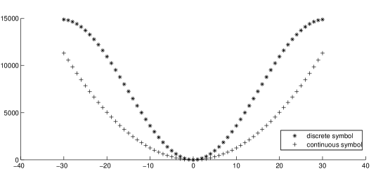
Figure 1. The discrete and continous symbols, $h=1/60$

Let $\{\widehat{u}_{0}(n)\}_{n=-N/2}^{N/2},$ be the Fourier coefficients of $\mathbf{u}^{h}(0)$. Thus $\mathbf{u}^{h}(0)$ writes as follows:

$$\mathbf{u}^{h}(0)=\sum_{n=-N/2}^{N/2}\widehat{u}_{0}(n)\boldsymbol{\varphi}^{h}_{n}.$$

Introducing this representation in equation (2.1) we find that the coefficients $\{\widehat{u}(t,n)\}$, $-N/2\leq n\leq N$, of $\mathbf{u}^{h}(t)$ satisfy the following ODE’s:

$$\left\{\begin{array}[]{ll}\displaystyle i\frac{d\widehat{u}(n,t)}{dt}+\widehat{u}(n,t)\frac{\exp(2i\pi nh)+\exp(-2i\pi nh)-2}{h^{2}}=0,&t>0,\\ \\ \widehat{u}(n,0)=\widehat{u}_{0}(n).&\end{array}\right.$$

Solving these ODE’s we obtain that the solution $\mathbf{u}^{h}$ of (2.1) is given by

(2.2) $$\mathbf{u}^{h}(t)=\sum_{n=-N/2}^{N/2}\widehat{u}_{0}(n)\exp\Big{(}-\frac{4it\sin^{2}(n\pi h)}{h^{2}}\Big{)}\boldsymbol{\varphi}^{h}_{n}$$

Observe that the in contrast with the continuous case, where the solutions are given by the following expression

$$u(t,x)=\sum_{n\in\mathbb{Z}}\widehat{u}_{0}(n)\exp(-4i\pi^{2}n^{2}t)\exp(2i\pi nx),$$

here the symbol $n^{2}$, $n\in\mathbb{Z}$, has been replaced by

(2.3) $$p_{h}(n)=\frac{4\sin^{2}\big{(}n\pi h\big{)}}{h^{2}}=4{(N+1)^{2}}\sin^{2}\Big{(}\frac{n\pi}{N+1}\Big{)},\,n=-\frac{N}{2},\dots,\frac{N}{2},$$

and the vectors $\boldsymbol{\varphi}_{n}^{h}$ are the projections of the exponentials $\exp(2i\pi kx)$ on the considered grid.

As we can see in Figure 1 the discrete symbol $p_{h}(n)$ introduced by scheme (2.1) changes convexity at the points $n=\pm(N+1)/4$. We recall that, in the case of Cauchy problem for LSE, this pathology of the discrete symbol has been used in [6] to prove the lack of uniform Strichartz estimates for the classical numerical approximation (1.6). It is then natural to expect that also in the periodic case the space time integrability of the solutions will be loosed in its simplest approximation scheme.

The following theorem shows the existence of initial data in $L^{2}$ for which the mixed $L^{4}$-norm of the approximate solutions blows-up as the mesh size tends to zero.

Theorem 2.1.

Let be $T>0$. Then the following holds:

(2.4) $$\sup_{h>0}\sup_{\mathbf{u}^{h}(0)\in L^{2}(\mathbb{T}_{h})}\frac{\|\mathbf{u}^{h}\|_{L^{4}(0,T;L^{4}(\mathbb{T}_{h}))}}{\|\mathbf{u}^{h}(0)\|_{L^{2}(\mathbb{T}_{h})}}=\infty,$$

where $\mathbf{u}^{h}$ is the solution of equation (2.1) with $\mathbf{u}^{h}(0)$ as initial datum.

Remark 2.2.

Let $\mathbf{P}^{h}$ be the piecewise constant interpolator. In view of Theorem 2.1, for any fixed $T>0$, the uniform boundedness principle guarantees the existence of a function $u(0)\in L^{2}(\mathbb{T^{1}})$ and a sequence $\mathbf{u}^{h}(0)$ such that $\mathbf{P}^{h}\mathbf{u}^{h}(0)\rightarrow u(0)$ in $L^{2}(\mathbb{T^{1}})$ such that the corresponding solutions $\mathbf{u}^{h}$ of (2.1) satisfy

$$\|\mathbf{P}^{h}\mathbf{u}^{h}\|_{L^{4}(0,T;L^{4}(\mathbb{T}^{1}))}\rightarrow\infty.$$

In what follows, to avoid the presence of constants, we will use the notation $A\lesssim B$ to report the inequality $A\leq constant\times B$, where the constant is independent of $h$. The statement $A\simeq B$ is equivalent to $A\lesssim B$ and $B\lesssim A$.

Proof of Theorem 2.1.

Let us fix $T>0$. We will consider initial data with their spectrum concentrated at the point $N/4$. A similar construction can be done for $-N/4$, this point having the same pathology as the previous one.

Let us fix $\alpha\in(0,1)$. We set

$$\Lambda_{N}=\Big{\{}n:|n|\leq\frac{N}{2},\,\Big{|}n-\frac{N}{4}\Big{|}<N^{\alpha}\Big{\}}.$$

To prove (2.4) we choose as initial datum in problem (2.1) the following function:

(2.5) $$\mathbf{u}^{h}(0)=\sum_{n\in\Lambda_{N}}\boldsymbol{\varphi}^{h}_{n}.$$

This function has all its Fourier coefficients identically one in $\Lambda_{N}$ and vanish outside this set. A similar construction has been done in [7] in the context of the analysis of the dispersive properties of the classical finite difference approximation of the Cauchy problem for the Schrödinger equation. By choosing initial data concentrated at the pathological points the solutions of the scheme will be more and more discrepant to its continuous counterpart.

Figure 2. Example of initial data chosen in (2.5), N=500, $\alpha=1/4$

Using the orthogonality of the vectors $\{\boldsymbol{\varphi}^{h}_{n}\}_{n=-N/2}^{N/2}$ we obtain the following behaviour of the $L^{2}$-norm of the initial datum:

(2.6) $$\|\mathbf{u}^{h}(0)\|_{L^{2}(\mathbb{T}_{h})}\simeq N^{\alpha/2}.$$

We will prove that the $L^{4}(0,T;L^{4}(\mathbb{T}_{h}))$-norm of

(2.7) $$\mathbf{u}^{h}(t)=\sum_{n\in\Lambda_{N}}\exp\Big{(}-\frac{4it\sin^{2}(n\pi h)}{h^{2}}\Big{)}\boldsymbol{\varphi}^{h}_{n},$$

solution of equation (2.1) with initial datum given by (2.5), increases faster than $N^{\alpha/2}$. To evaluate the $L^{4}(0,T;L^{4}(\mathbb{T}_{h}))$-norm of $\mathbf{u}^{h}$ we will use that for any vector $\mathbf{v}$ given by

$$\mathbf{v}=\sum_{n=-N/2}^{N/2}\widehat{a}(n)\boldsymbol{\varphi}^{h}_{n}$$

its $L^{4}(\mathbb{T}_{h})$-norm satisfies

(2.8) $$\|\mathbf{v}\|^{4}_{L^{4}(\mathbb{T}_{h})}=\sum_{\begin{subarray}{c}-N/2\leq n_{i}\leq N/2\\ n_{1}+n_{2}=n_{3}+n_{4}\end{subarray}}\widehat{a}(n_{1})\widehat{a}({n_{2}})\overline{\widehat{a}}(n_{3})\overline{\widehat{a}}(n_{4})$$

The proof of (2.8) uses only the orthogonality of the vectors $\boldsymbol{\varphi}^{h}_{n}$ and we will omit it. Applying this result to the solution $\mathbf{u}^{h}$ written in the form (2.2) we get

$$\|\mathbf{u}^{h}\|_{L^{4}(0,T;\mathbb{T}_{h})}^{4}=\int_{0}^{T}\sum_{\begin{subarray}{c}n_{i}\in\Lambda_{N}\\ n_{1}+n_{2}=n_{3}+n_{4}\end{subarray}}e^{-itq_{h}(\mathbf{n})}dt,$$

where the function $q_{h}(\mathbf{n})$ is given by

(2.9) $$q_{h}(\mathbf{n})=p_{h}(n_{1})+p_{h}(n_{2})-p_{h}(n_{3})-p_{h}(n_{4}),\,\mathbf{n}=(n_{1},n_{2},n_{3},n_{4}).$$

Using that the function $q_{h}$ satisfies $q_{h}(n_{1},n_{2},n_{3},n_{4})=-q_{h}(n_{3},n_{4},n_{1},n_{2})$ we have

$$\|\mathbf{u}^{h}\|_{L^{4}(0,T;\,L^{4}(\mathbb{T}_{h}))}^{4} =\frac{1}{2}\sum_{\begin{subarray}{c}n_{i}\in\Lambda_{N}\\ n_{1}+n_{2}=n_{3}+n_{4}\end{subarray}}\int_{0}^{T}(e^{-itq_{h}(n_{1},n_{2},n_{3},n_{4})}+e^{-itq_{h}(n_{3},n_{4},n_{1},n_{2})})dt$$

$$=\sum_{\begin{subarray}{c}n_{i}\in\Lambda_{N}\\ n_{1}+n_{2}=n_{3}+n_{4}\end{subarray}}\int_{0}^{T}\cos(tq_{h}(\mathbf{n}))dt$$

We will prove that for large enough $N$, the term $q_{h}(\mathbf{n})$ occurring in the right hand side is sufficiently small and then all the integrals occurring in the last sum behaves as $T$.

Explicit computations show that for any $\mathbf{n}=(n_{1},n_{2},n_{3},n_{4})$ with $n_{1}+n_{2}=n_{3}+n_{4}$ the following holds:

$$q_{h}(\mathbf{n})=8(N+1)^{2}\cos \Big{(}\frac{(n_{1}+n_{2})\pi}{N+1}\Big{)}\sin\Big{(}\frac{(n_{1}-n_{2}+n_{3}-n_{4})\pi}{2(N+1)}\Big{)}\sin\Big{(}\frac{(n_{1}-n_{2}-n_{3}+n_{4})\pi}{2(N+1)}\Big{)}.$$

We estimate each term in the above representation of $q_{h}(\mathbf{n})$. Using that $n_{1}$ and $n_{2}$ belong to $\Lambda_{N}$ we get

$$\left|\frac{(n_{1}+n_{2})\pi}{N+1}-\frac{\pi}{2}\right|\leq\left|\frac{n_{1}\pi}{N+1}-\frac{\pi}{4}\right|+\left|\frac{n_{2}\pi}{N+1}-\frac{\pi}{4}\right|\leq\frac{2\pi(N^{\alpha}+1/4)}{(N+1)}\lesssim\frac{1}{(N+1)^{1-\alpha}}.$$

Thus

(2.10) $$\left|\cos\Big{(}\frac{(n_{1}+n_{2})\pi}{N+1}\Big{)}\right|\lesssim\sin\Big{(}\frac{1}{(N+1)^{1-\alpha}}\Big{)}\lesssim\frac{1}{(N+1)^{1-\alpha}}.$$

Also using that $|n_{1}-n_{2}|+|n_{3}-n_{4}|\leq 4(N+1)^{\alpha}$ we obtain that

(2.11) $$\left|\sin\Big{(}\frac{(n_{1}-n_{2}+n_{3}-n_{4})\pi}{2(N+1)}\Big{)}\sin\Big{(}\frac{(n_{1}-n_{2}-n_{3}+n_{4})\pi}{2(N+1)}\Big{)}\right|\lesssim\frac{1}{(N+1)^{2-2\alpha}}.$$

In view of inequalities (2.10) and (2.11) we obtain that $q_{h}(\mathbf{n})$ satisfies $|q_{h}(\mathbf{n})|\lesssim N^{3\alpha-1}$ for any $\mathbf{n}=(n_{1},n_{2},n_{3},n_{4})\in\Lambda_{N}^{4}$ with $n_{1}+n_{2}=n_{3}+n_{4}$. Choosing $\alpha<1/3$ the following estimate holds uniformly for all $\mathbf{n}$ as above:

$$\int_{0}^{T}\cos(tq_{h}(\mathbf{n}))dt\geq T\cos\Big{(}\frac{T}{N^{1-3\alpha}}\Big{)}\gtrsim 1.$$

Using that the number of pairs $\mathbf{n}\in\Lambda_{N}^{4}$ with $n_{1}+n_{2}=n_{3}+n_{4}$ is of order $|\Lambda_{N}|^{3}$ we obtain that that

(2.12) $$\|\mathbf{u}^{h}\|_{L^{4}(0,T;\,L^{4}(\mathbb{T}_{h}))}\simeq N^{3\alpha/4}.$$

By (2.6) and (2.12) we finally obtain that

$$\frac{\|\mathbf{u}^{h}\|_{L^{4}(0,T;\,L^{4}(\mathbb{T}_{h}))}}{\|\mathbf{u}^{h}(0)\|_{l^{2}(\mathbb{T}_{h})}}\simeq N^{\alpha/4}$$

which finishes the proof. ∎

3. Filtering the high frequencies

In this section we prove that a spectral filtering of the initial data will provides uniform $L^{4}$-estimates for the discrete solutions. The following Theorem shows that this holds for all initial data supported far away from the pathological spectral points $\pm N/4$.

Theorem 3.1.

Let $\lambda<1/4$. There is a positive constant $c(\lambda)$ such that for all initial datum $\mathbf{u}^{h}(0)\in{\rm{Span}}\{\varphi_{n}^{h}:|n|\leq\lambda N\}$, the solution $\mathbf{u}^{h}$ of equation (2.1) satisfies

(3.1) $$\|\mathbf{u}^{h}\|_{L^{4}(0,T;\,L^{4}(\mathcal{\mathbb{T}}_{h}))}\leq c(\lambda)\|\mathbf{u}^{h}(0)\|_{L^{2}(\mathbb{T}_{h})}.$$

Remark 3.2.

The same result holds if for some positive constant $\epsilon$ the initial datum $\mathbf{u}^{h}(0)$ belongs to the set

$${\rm{Span}}\Big{\{}\varphi_{n}^{h}:\Big{|}|n|-\frac{N}{4}\Big{|}\geq\epsilon N\Big{\}}.$$

On this set the symbol introduced by the finite difference scheme (2.1) is uniformly convex, with a parameter which depends by $\epsilon$. Clearly, this uniform convexity is lost as $\epsilon$ goes to zero.

The main ingredient in the proof of the above result is the following direct Ingham’s inequality.

Lemma 3.3.

Let $(\mu_{n})_{n\in\mathbb{Z}}$ be a sequence of real numbers and $\gamma>0$ be such

(3.2) $$\mu_{n+1}-\mu_{n}\geq\gamma>0,\,\forall n\in\mathbb{Z}.$$

For any $T>0$ there exists a positive constant $C=C(T,\gamma)>0$ such that, for any finite sequence $(a_{n})_{n\in Z}$,

(3.3) $$\int_{-T}^{T}\Big{|}\sum_{n}a_{n}e^{i\mu_{n}t}\Big{|}^{2}dt\leq C\sum_{n}|a_{n}|^{2}.$$

The Ingham’s inequalities have been successfully used to prove observability inequalities in for many 1-D control problems. They generalize the classical Parseval equality for orthogonal sequences. We refer to Young [14] to a survey on the theme.

Proof of Theorem 3.1.

Let us consider $\mathbf{u}^{h}(0)\in{\rm{Span}}\{\varphi_{n}^{h}:|n|\leq\lambda N\}$ as initial data in equation (2.1):

$$\mathbf{u}^{h}(0)=\sum_{|n|\leq\lambda N}\widehat{u}_{0}(n)\boldsymbol{\varphi}^{h}_{n}.$$

The solution of (2.1) is given by

$$\mathbf{u}^{h}(t)=\sum_{|n|\leq\lambda N}\widehat{u}_{0}(n)\exp(-itp_{h}(n))\boldsymbol{\varphi}^{h}_{n}$$

where $p_{h}(n)=4/{h^{2}}\sin^{2}(n\pi h)$.

With $q_{h}$ as in (2.9), identity (2.8) applied to vector $\mathbf{u}^{h}$ gives us

$$\|\mathbf{u}^{h}\| {}^{4}_{L^{4}(0,T;\,L^{4}(\mathbb{T}_{h})}=\int_{0}^{T}\sum_{\begin{subarray}{c}|n_{i}|\leq\lambda N\\ n_{1}+n_{2}=n_{3}+n_{4}\end{subarray}}\widehat{u}_{0}(n_{1})\widehat{u}_{0}(n_{2})\overline{\widehat{u}}_{0}(n_{3})\overline{\widehat{u}}_{0}(n_{4})e^{-itq_{h}(\mathbf{n})}$$

$$=\int_{0}^{T}\sum_{|r|\leq 2\lambda N}\sum_{\begin{subarray}{c}|n_{i}|\leq\lambda N\\ n_{1}+n_{2}=r,\,n_{3}+n_{4}=r\end{subarray}}\widehat{u}_{0}(n_{1})\widehat{u}_{0}(n_{2})\overline{\widehat{u}}_{0}(n_{3})\overline{\widehat{u}}_{0}(n_{4})e^{-itq_{h}(\mathbf{n})}$$

$$=\sum_{|r|\leq 2\lambda N}\int_{0}^{T}\Big{|}\sum_{\begin{subarray}{c}|n_{i}|\leq\lambda N\\ n_{1}+n_{2}=r\end{subarray}}\widehat{u}_{0}(n_{1})\widehat{u}_{0}(n_{2})e^{-it(p_{h}(n_{1})+p_{h}(n_{2}))}\Big{|}^{2}dt.$$

It is sufficient to prove that for any $|r|\leq 2\lambda N$, $\Sigma(r)$ defined by

$$\Sigma(r)=\int_{0}^{T}\Big{|}\sum_{\begin{subarray}{c}|n_{i}|\leq\lambda N\\ n_{1}+n_{2}=r\end{subarray}}\widehat{u}_{0}(n_{1})\widehat{u}_{0}(n_{2})e^{-it(p_{h}(n_{1})+p_{h}(n_{2}))}\Big{|}^{2}dt$$

satisfies

(3.4) $$\Sigma(r)\leq\sum_{\begin{subarray}{c}|n_{i}|\leq\lambda N\\ n_{1}+n_{2}=r\end{subarray}}|\widehat{u}_{0}(n_{1})|^{2}|\widehat{u}_{0}(n_{2})|^{2}.$$

We consider the case $r\geq 0$ the other case being similar. We write $\Sigma(r)$ as

(3.5) $$\Sigma(r)=\int_{0}^{T}\Big{|}\sum_{r-\lambda N\leq n\leq\lambda N}\widehat{u}_{0}(n)\widehat{u}_{0}(r-n)e^{it\mu_{h}(n)}\Big{|}^{2}dt$$

where $\mu_{h}(n)=-p_{h}(n)-p_{h}(r-n)$.

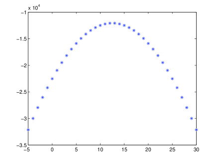
Figure 3. The sequence $\mu_{h}(n)$, $N=150$, $\lambda=1/5$, $r=N/6$, $n=r-\lambda N,\dots,\lambda N$

In order to apply Ingham’s inequality (3.3) we need to prove that the sequence $\mu_{h}(n)$ satisfies the gap condition (3.2). As we can see in Figure 3, there are two range of $n$’s for which the gap condition (3.2) is satisfied in each of them.

Elementary manipulations of trigonometric functions give us that

(3.6) $$\mu_{h}(n+1)-\mu_{h}(n)=8(N+1)^{2}\cos\Big{(}\frac{\pi r}{N+1}\Big{)}\sin\Big{(}\frac{\pi(r-2n-1)}{N+1}\Big{)}\sin\Big{(}\frac{\pi}{N+1}\Big{)}.$$

Thus the sequence $\mu_{h}(n)$ satisfies the following inequalities:

$$\mu_{h}(r-[\lambda N])<\mu_{h}(r-[\lambda n]+1)<\dots<\mu_{h}\Big{(}\Big{[}\frac{r}{2}\Big{]}-1\Big{)}<\mu_{h}\Big{(}\Big{[}\frac{r}{2}\Big{]}\Big{)}$$

and

$$\mu_{h}\Big{(}\Big{[}\frac{r}{2}\Big{]}+1\Big{)}>\mu_{h}\Big{(}\Big{[}\frac{r}{2}\Big{]}+2\Big{)}>\dots>\mu_{h}(\lambda N),$$

where $[\cdot]$ represents the floor function.

By (3.6), for any $n\leq[r/2]-1$ in the definition (3.5) of $\Sigma(r)$ we obtain

$$\mu_{h}(n+1)-\mu_{h}(n)\geq 8(N+1)^{2}\cos(2\lambda\pi)\sin^{2}\Big{(}\frac{\pi}{N+1}\Big{)}\geq c_{1}(\lambda).$$

Also, for $n\geq[r/2]$ the following holds

$$\mu_{h}(n+1)-\mu_{h}(n)\leq-8(N+1)^{2}\cos(2\lambda\pi)\sin^{2}\Big{(}\frac{\pi}{N+1}\Big{)}\leq-c_{2}(\lambda).$$

This suggests us to split the right hand side of (3.5) as $\Sigma(r)=\Sigma_{1}(r)+\Sigma_{2}(r)$ where

$$\Sigma_{1}(r)=\int_{0}^{T}\Big{|}\sum_{n=r-\lambda N}^{[r/2]}\widehat{u}_{0}(n)\widehat{u}_{0}({r-n})e^{it\mu_{h}(n)}\Big{|}^{2}dt$$

and

$$\Sigma_{2}(r)=\int_{0}^{T}\Big{|}\sum_{n=[r/2]+1}^{\lambda N}\widehat{u}_{0}(n)\widehat{u}_{0}({r-n})e^{it\mu_{h}(n)}\Big{|}^{2}dt.$$

For each of the above terms we apply Ingham’s inequality and obtain:

$$\Sigma_{1}(r)\leq\sum_{r-\lambda N\leq n}^{[r/2]}|\widehat{u}_{0}(n)|^{2}|\widehat{u}_{0}(r-n)|^{2}$$

and

$$\Sigma_{2}(r)\leq\sum_{[r/2]+1}^{\lambda N}|\widehat{u}_{0}(n)|^{2}|\widehat{u}_{0}(r-n)|^{2}$$

The last two estimates show that (3.4) holds and then (3.1). The proof is now complete. ∎

4. A viscous scheme

In this section we will analyze the $L^{4}$-property for numerical schemes that contain artificial numerical viscosity.

The scheme we will analyze is as follows:

(4.1) $$\left\{\begin{array}[]{lc}\displaystyle i\frac{du_{j}}{dt}+\frac{u^{h}_{j+1}-2u^{h}_{j}+u^{h}_{j-1}}{h^{2}}=ia(h)\frac{u^{h}_{j+1}-2u^{h}_{j}+u^{h}_{j-1}}{h^{2}},&j=0,\dots,N,\,t>0,\\ \\ u_{0}(t)=u_{N+1}(t),&t>0,\\ \end{array}\right.$$

where by convention $u_{-1}=u_{N}$.

The main result of this section is given by the following theorem.

Theorem 4.1.

Let $a(h)$ be such that

(4.2) $$\inf_{h>0}\frac{a(h)}{h}>0.$$

For any positive time $T$, there exists a positive constant $C(T)$ such that

(4.3) $$\|\mathbf{u}^{h}\|_{L^{4}(0,T;\,L^{4}(\mathbb{T}_{h}))}\leq C(T)\|\mathbf{u}^{h}(0)\|_{L^{2}(\mathbb{T}_{h})}$$

holds for all $\mathbf{u}^{h}(0)\in L^{2}(\mathbb{T}_{h})$, uniformly in $h>0$.

Remark 4.2.

We do not know whether condition (4.2) on $a(h)$ is necessary. It is an open problem to determine the range of $\beta>1$, if there exists any, such that for $a(h)=h^{\beta}$ the result of the above theorem still holds.

Proof.

Tacking the DFT in (4.1) we find that the Fourier coefficients of $\mathbf{u}^{h}(t)$, $\widehat{u}(t,k)$, $k=-N/2,\dots,N/2$ solve the following ODE’s:

$$\left\{\begin{array}[]{ll}\displaystyle i\frac{d\widehat{u}(t,k)}{dt}+\widehat{u}(t,k)p_{h}(n)=ia(h)\widehat{u}(t,k)p_{h}(n),\,t>0.\\ \\ \widehat{u}(0,k)=\widehat{u}_{0}(k),\end{array}\right.$$

where $\widehat{u}_{0}(k),k=-N/2,\dots,N/2$ are the Fourier coefficients of $\mathbf{u}^{h}(0)$:

$$\mathbf{u}^{h}(0)=\sum_{|n|\leq N/2}\widehat{u}_{0}(n)\boldsymbol{\varphi}_{n}^{h}.$$

Solving the above ODE’s we obtain that $\mathbf{u}^{h}$, the solution of (4.1) is as follows

$$\mathbf{u}^{h}(t)=\sum_{k=-N/2}^{N/2}\widehat{u}_{0}(k)\exp\left(-\frac{4it\sin^{2}(k\pi h)}{h^{2}}-a(h)\frac{4t\sin^{2}(k\pi h)}{h^{2}}\right)\boldsymbol{\varphi}_{k}^{h}.$$

We split $\mathbf{u}^{h}$ in two components $\mathbf{u}^{h}(t)=\mathbf{u}^{h}_{low}(t)+\mathbf{u}^{h}_{high}(t),$ corresponding to a low:

(4.4) $$\mathbf{u}^{h}_{low}(t)=\sum_{|k|\leq N/8}\widehat{u}_{0}(k)\exp\left(-itp_{h}(n)-a(h)tp_{h}(n)\right)\boldsymbol{\varphi}_{k}^{h},$$

respectively high frequencies component of $\mathbf{u}^{h}$:

(4.5) $$\mathbf{u}^{h}_{high}(t)=\sum_{N/8<|k|\leq N/2}\widehat{u}_{0}(k)\exp\left(-itp_{h}(n)-a(h)tp_{h}(n)\right)\boldsymbol{\varphi}_{k}^{h}.$$

The choice of $N/8$ as the range of low frequencies is motivated by the fact that there are solutions concentrated near the point $N/4$ of the spectrum that generate the blow-up of the $L^{4}(0,T;\,L^{4}(\mathbb{T}_{h}))$-norm as we have seen in Section 2.

In the following we will prove that the two components $\mathbf{u}^{h}_{low}$ and $\mathbf{u}^{h}_{low}$ of $\mathbf{u}^{h}$ satisfy:

$$\|\mathbf{u}^{h}_{low}\|_{L^{4}(0,T;\,L^{4}(\mathbb{T}_{h}))}\lesssim\|\mathbf{u}^{h}_{low}(0)\|_{L^{2}(\mathbb{T}_{h})}$$

and

$$\|\mathbf{u}^{h}_{high}\|_{L^{4}(0,T;\,L^{4}(\mathbb{T}_{h}))}\lesssim\|\mathbf{u}^{h}_{high}(0)\|_{L^{2}(\mathbb{T}_{h})}.$$

Step I. Estimate of $\mathbf{u}_{high}^{h}$. Using identity (2.8) we obtain that $\mathbf{u}^{h}_{high}$ satisfies the rough estimate

$$\|\mathbf{u}_{high}^{h}\|^{4}_{L^{4}(0,T;\,L^{4}(\mathbb{T}_{h}))} \leq\sum_{\begin{subarray}{c}N/8<|n_{i}|\leq N/2\\ n_{1}+n_{2}=n_{3}+n_{4}\end{subarray}}|\widehat{u}_{0}(n_{1})\widehat{u}_{0}(n_{2})\widehat{u}_{0}(n_{3})\widehat{u}_{0}(n_{4})|\int_{0}^{T}e^{-ta(h)\sigma_{h}(\bf n)}dt$$

$$\leq\sum_{\begin{subarray}{c}N/8<|n_{i}|\leq N/2\\ n_{1}+n_{2}=n_{3}+n_{4}\end{subarray}}\frac{|\widehat{u}_{0}(n_{1})\widehat{u}_{0}(n_{2})\widehat{u}_{0}(n_{3})\widehat{u}_{0}(n_{4})|}{a(h)\sigma_{h}(\bf n)}.$$

where $\sigma_{h}$ is given by

$$\sigma_{h}(\mathbf{n})=p_{h}(n_{1})+p_{h}(n_{2})+p_{h}(n_{3})+p_{h}(n_{4}),\,\mathbf{n}=(n_{1},n_{2},n_{3},n_{4}).$$

Observe that for all $\textbf{n}=(n_{1},n_{2},n_{3},n_{4})$ with $N/8<n_{i}\leq N/2$, $\sigma_{h}(\mathbf{n})$ can be bounded from below as follows:

$$\sigma_{h}(\mathbf{n})\geq{16}(N+1)^{2}\sin^{2}\Big{(}\frac{N\pi}{8(N+1)}\Big{)}\geq c_{1}(N+1)^{2}.$$

Thus, in the above inequality we replace $\sigma_{h}(\mathbf{n})$ by $(N+1)^{2}$ and we obtain

(4.6) $$\|\mathbf{u}_{high}^{h}\|^{4}_{L^{4}(0,T;\,L^{4}(\mathbb{T}_{h}))}\lesssim\frac{h^{2}}{a(h)}\sum_{\begin{subarray}{c}N/8<|n_{i}|\leq N/2\\ n_{1}+n_{2}=n_{3}+n_{4}\end{subarray}}|\widehat{u}_{0}(n_{1})\widehat{u}_{0}(n_{2})\widehat{u}_{0}(n_{3})\widehat{u}_{0}(n_{4})|.$$

The right hand side sum satisfies:

$$\sum_{\begin{subarray}{c}N/8<|n_{i}|\leq N/2\\ n_{1}+n_{2}=n_{3}+n_{4}\end{subarray}}|\widehat{u}_{0}(n_{1})\widehat{u}_{0}(n_{2}) \widehat{u}_{0}(n_{3})\widehat{u}_{0}(n_{4})|\leq\sum_{N/4<r\leq N}\Big{(}\sum_{\begin{subarray}{c}N/8<|n_{i}|\leq N/2\\ n_{1}+n_{2}=r\end{subarray}}|\widehat{u}_{0}(n_{1})\widehat{u}_{0}(n_{2})|\Big{)}^{2}$$

$$\lesssim\sum_{N/4<r\leq N}(r+1)\sum_{\begin{subarray}{c}N/8<|n_{i}|\leq N/2\\ n_{1}+n_{2}=r\end{subarray}}|\widehat{u}_{0}(n_{1})\widehat{u}_{0}(n_{2})|^{2}$$

(4.7) $$\lesssim(N+1)\Big{(}\sum_{N/8\leq n\leq N/2}|\widehat{u}_{0}(n)|^{2}\Big{)}^{2}.$$

Estimates (4.6) and (4) imply that

$$\|\mathbf{u}_{high}^{h}\|^{4}_{L^{4}(0,T;\,L^{4}(\mathbb{T}_{h}))}\lesssim\frac{h}{a(h)}{\|\mathbf{u}_{high}^{h}(0)\|_{L^{2}(\mathbb{T}_{h})}^{4}}.$$

In view of assumption (4.2) on $a(h)$ we obtain that the high frequencies component of $\mathbf{u}^{h}$, $\mathbf{u}^{h}_{high}$, satisfies the following estimate:

$$\|\mathbf{u}_{high}^{h}\|_{L^{4}(0,T;\,L^{4}(\mathbb{T}_{h}))}\lesssim\|\mathbf{u}_{high}^{h}(0)\|_{L^{2}(\mathbb{T}_{h})}.$$

Step II. Estimate of $\mathbf{u}_{low}^{h}$. Using the same ideas as above the low frequencies component $\mathbf{u}_{low}^{h}$ satisfies:

$$\|\mathbf{u}_{low}^{h}\|^{4}_{L^{4}(0,T;\,L^{4}(\mathbb{T}_{h}))} =\int_{0}^{T}\sum_{\begin{subarray}{c}|n_{i}|\leq N/8\\ n_{1}+n_{2}=n_{3}+n_{4}\end{subarray}}\widehat{u}_{0}(n_{1})\widehat{u}_{0}(n_{2})\overline{\widehat{u}}_{0}(n_{3})\overline{\widehat{u}}_{0}(n_{4})e^{-itq_{h}(\mathbf{n})}e^{-ta(h)\sigma_{h}(\mathbf{n})}dt$$

$$=\int_{0}^{T}\sum_{|r|\leq N/4}\sum_{\begin{subarray}{c}|n_{i}|\leq N/8\\ n_{1}+n_{2}=n_{3}+n_{4}=r\end{subarray}}\widehat{u}_{0}(n_{1})\widehat{u}_{0}(n_{2})\overline{\widehat{u}}_{0}(n_{3})\overline{\widehat{u}}_{0}(n_{4})e^{-itq_{h}(\mathbf{n})}e^{-ta(h)\sigma_{h}(\mathbf{n})}dt$$

$$=\int_{0}^{T}\sum_{|r|\leq N/4}\Big{|}\sum_{\begin{subarray}{c}|n_{i}|\leq N/8\\ n_{1}+n_{2}=r\end{subarray}}\widehat{u}_{0}(n_{1})\widehat{u}_{0}(n_{2})e^{-it(p_{h}(n_{1})+p_{h}(n_{2}))}e^{-ta(h)(p_{h}(n_{1})+p_{h}(n_{2}))}\Big{|}^{2}dt.$$

It is sufficient to prove the existence of a positive constant $c$, independent of $|r|\leq N/4$ and $N$, such that $\Sigma(r)$ defined by

(4.8) $$\Sigma(r)=\int_{0}^{T}\Big{|}\sum_{\begin{subarray}{c}|n_{i}|\leq N/8\\ n_{1}+n_{2}=r\end{subarray}}\widehat{u}_{0}(n_{1})\widehat{u}_{0}(n_{2})e^{-it(p_{h}(n_{1})+p_{h}(n_{2}))}e^{-ta(h)(p_{h}(n_{1})+p_{h}(n_{2}))}\Big{|}^{2}dt,$$

satisfies the following inequality:

(4.9) $$\Sigma(r)\leq c\sum_{\begin{subarray}{c}|n_{i}|\leq N/8\\ n_{1}+n_{2}=r\end{subarray}}|\widehat{u}_{0}(n_{1})|^{2}|\widehat{u}_{0}(n_{2})|^{2}.$$

We consider the case $r\geq 0$, the other case cans be treated in a similar manner. The conditions imposed on $r,n_{1},n_{2}$ in definition (4.8) of $\Sigma(r)$ give us that $n_{1}$ satisfies:

$$-\frac{N}{8}\leq r-\frac{N}{8}\leq n_{1}\leq\frac{N}{8}\leq r+\frac{N}{8}.$$

This allows us to rewrite $\Sigma(r)$ in the following form

$$\Sigma(r)=\int_{0}^{T}\Big{|}\sum_{n=\,r-N/8}^{N/8}\widehat{u}_{0}(n)\widehat{u}_{0}(r-n)e^{-it(p_{h}(n)+p_{h}(r-n))}e^{-ta(h)(p_{h}(n)+p_{h}(r-n))}\Big{|}^{2}dt.$$

Using that $r-{N}/8\leq r/2\leq{N}/8$ we write $\Sigma(r)\leq 2(\Sigma_{1}(r)+\Sigma_{2}(r))$ where

$$\Sigma_{1}(r)=\int_{0}^{T}\Big{|}\sum_{n=\,r-N/8}^{[r/2]}\widehat{u}_{0}(n)\widehat{u}_{0}(r-n)e^{-it(p_{h}(n)+p_{h}(r-n))}e^{-ta(h)(p_{h}(n)+p_{h}(r-n))}\Big{|}^{2}dt$$

and

$$\Sigma_{2}(r)=\int_{0}^{T}\Big{|}\sum_{n=[r/2]+1}^{N/8}\widehat{u}_{0}(n)\widehat{u}_{0}(r-n)e^{-it(p_{h}(n)+p_{h}(r-n))}e^{-ta(h)(p_{h}(n)+p_{h}(r-n))}\Big{|}^{2}dt.$$

In the following we prove that

$$\Sigma_{1}(r)\lesssim C(T)\sum_{n=r-N/8}^{[r/2]}|\widehat{u}_{0}(n)|^{2}|\widehat{u}_{0}(r-n)|^{2}.$$

In a similar manner $\Sigma_{2}(r)$ will satisfy

$$\Sigma_{2}(r)\lesssim C(T)\sum_{n=[r/2]+1}^{N/8}|\widehat{u}_{0}(n)|^{2}|\widehat{u}_{0}(r-n)|^{2}$$

and thus (4.9) holds, which finishes the proof.

With the notations $\mu_{h}(n,m)=q_{h}(n,r-n,m,r-m)$ and $\nu_{h}(n,m)=\sigma_{h}(n,r-n,m,r-m)$ we get

$$\Sigma_{1}(r) \leq \sum_{n=\,r-N/8}^{[r/2]}|\widehat{u}_{0}(n)|^{2}|\widehat{u}_{0}(r-n)|^{2}\int_{0}^{T}e^{-ta(h)\nu_{h}(n,m)}dt+S_{1}(r)$$

$$\leq T\sum_{n=r-N/8}^{[r/2]}|\widehat{u}_{0}(n)|^{2}|\widehat{u}_{0}(r-n)|^{2}+S_{1}(r).$$

where

$$S_{1}(r)=\sum_{\begin{subarray}{c}n,m=r-N/8\\ n\neq m\end{subarray}}^{[r/2]}|\widehat{u}_{0}(n)\widehat{u}_{0}(r-n){\widehat{u}}_{0}(m){\widehat{u}}_{0}(r-m)|\left|\int_{0}^{T}e^{-it\mu_{h}(n,m)}e^{-ta(h)\nu_{h}(n,m)}dt\right|$$

It is sufficient to prove that

(4.10) $$S_{1}(r)\lesssim\sum_{n=r-N/8}^{[r/2]}|\widehat{u}_{0}(n)|^{2}|\widehat{u}_{0}(r-n)|^{2}.$$

Observe that $S_{1}$ satisfies the following estimate :

$$S_{1}(r) \leq 2\sum_{\begin{subarray}{c}n,m=r-N/8\\ n\neq m\end{subarray}}^{[r/2]}\frac{|\widehat{u}_{0}(n)\widehat{u}_{0}(r-n){\widehat{u}}_{0}(m){\widehat{u}}_{0}(r-m)|}{|i\mu_{h}(n,m)+a(h)\nu_{h}(n,m)|}$$

$$=\sum_{n=r-N/8}^{[r/2]}|\widehat{u}_{0}(n)|^{2}|\widehat{u}_{0}(r-n)|^{2}\sum_{\begin{subarray}{c}m=r-N/8\\ m\neq n\end{subarray}}^{[r/2]}\frac{1}{|\mu_{h}(m,n)|}$$

$$\qquad+\sum_{m=r-N/8}^{[r/2]}|\widehat{u}_{0}(m)|^{2}|\widehat{u}_{0}(r-m)|^{2}\sum_{\begin{subarray}{c}n=r-N/8\\ n\neq m\end{subarray}}^{[r/2]}\frac{1}{|\mu_{h}(m,n)|}.$$

We prove the existence of a positive constant $C$, independent of $N$ and $r$ such that the following

$$l(n)=\sum_{\begin{subarray}{c}m=r-N/8\\ m\neq n\end{subarray}}^{[r/2]}\frac{1}{|\mu_{h}(m,n)|}\leq C$$

holds for all $n=r-N/8,\dots,[r/2]$. Thus (4.10) holds and the proof is finishes.

We claim the existence of a positive constant $c$ such that $\mu_{h}$ verifies

(4.11) $$|\mu_{h}(n,m)|\geq c|n-m||r-m-n|$$

for all $n,m\in I(r,N)=\{r-N/8,\dots,[r/2]\}$. Thus for a fixed $n$, $l(n)$ satisfies

$$l(n)\lesssim\sum_{\begin{subarray}{c}m=r-N/8\\ m\neq n\end{subarray}}^{[r/2]}\frac{1}{|n-m|^{2}}+\sum_{\begin{subarray}{c}m=r-N/8\\ m\neq n\end{subarray}}^{[r/2]}\frac{1}{|r-m-n|^{2}}\lesssim\sum_{m\geq 1}\frac{1}{m^{2}}\leq C.$$

It remains to prove (4.11). Explicit computations show that

$$\mu_{h}(n,m)=8(N+1)^{2}\cos\Big{(}\frac{r\pi}{N+1}\Big{)}\sin\Big{(}\frac{(r-m-n)\pi}{N+1}\Big{)}\sin\Big{(}\frac{(n-m)\pi}{N+1}\Big{)}.$$

Taking into account that $r\leq N/4$ we get $|\cos(r\pi/(N+1))|\geq\cos(\pi/4)$. This was the key point in choosing the low frequency component up to $N/8$. If we would have chosen all the frequencies up to $N/4$ we will obtain that $r\leq N/2$ and then the term $\cos(r\pi/N)$ could not be bounded from bellow by a positive constant. Using that $n$ and $m$ belong to $I(r,N)$ and that $r$ is nonnegative we have $|n|\leq N/8$ and $|m|\leq N/8$. Thus $|n-m|\leq N/4$ and

$$\Big{|}\sin\Big{(}\frac{(n-m)\pi}{N+1}\Big{)}\Big{|}\gtrsim\frac{|n-m|}{N+1}.$$

Also $r\leq N/4$ implies that $|r-m-n|\pi/(N+1)\leq\pi/2$ and

$$\Big{|}\sin\Big{(}\frac{(r-m-n)\pi}{N+1}\Big{)}\Big{|}\gtrsim\frac{|r-n-m|}{N+1}.$$

The last two inequalities prove (4.11).

The proof is now complete. ∎

References

- [1] J. Bourgain, Fourier transform restriction phenomena for certain lattice subsets and applications to nonlinear evolution equations. I. Schrödinger equations, Geom. Funct. Anal. 3 (1993), no. 2, 107–156.
- [2] by same author, Global solutions of nonlinear Schrödinger equations, American Mathematical Society Colloquium Publications, vol. 46, American Mathematical Society, Providence, RI, 1999.
- [3] N. Burq, P. Gérard, and N. Tzvetkov, Strichartz inequalities and the nonlinear Schrödinger equation on compact manifolds, Amer. J. Math. 126 (2004), no. 3, 569–605.
- [4] J. Ginibre and G. Velo, The global Cauchy problem for the nonlinear Schrödinger equation revisited, Ann. Inst. H. Poincaré Anal. Non Linéaire 2 (1985), no. 4, 309–327.
- [5] L.I. Ignat, Fully discrete schemes for the Schrödinger equation. Dispersive properties, M3AS, to appear.
- [6] L.I. Ignat and E. Zuazua, Dispersive properties of a viscous numerical scheme for the Schrödinger equation., C. R. Acad. Sci. Paris, Ser. I 340 (2005), no. 7, 529–534.
- [7] by same author, Dispersive properties of numerical schemes for nonlinear Schrödinger equations, Foundations of Computational Matehmatics, Santander 2005. L. M. Pardo et al. eds, vol. 331, London Mathematical Society Lecture Notes, 2006, pp. 181–207.
- [8] by same author, Numerical dispersive schemes for the nonlinear Schrödinger equation, preprint (2007).
- [9] M. Nixon, The discretized generalized Korteweg-de Vries equation with fourth order nonlinearity, J. Comput. Anal. Appl. 5 (2003), no. 4, 369–397.
- [10] A. Stefanov and P.G. Kevrekidis, Asymptotic behaviour of small solutions for the discrete nonlinear Schrödinger and Klein-Gordon equations, Nonlinearity 18 (2005), no. 4, 1841–1857.
- [11] R.S. Strichartz, Restrictions of Fourier transforms to quadratic surfaces and decay of solutions of wave equations., Duke Math. J. 44 (1977), 705–714.
- [12] L.N. Trefethen, Spectral methods in MATLAB, Software, Environments, and Tools, Society for Industrial and Applied Mathematics (SIAM), Philadelphia, PA, 2000.
- [13] Y. Tsutsumi, -solutions for nonlinear Schrödinger equations and nonlinear groups., Funkc. Ekvacioj, Ser. Int. 30 (1987), 115–125.
- [14] R.M. Young, An introduction to nonharmonic Fourier series, first ed., Academic Press Inc., San Diego, CA, 2001.
- [15] A. Zygmund, On Fourier coefficients and transforms of functions of two variables, Studia Math. 50 (1974), 189–201.