Learning deep linear neural networks: Riemannian gradient flows and convergence to global minimizers

Abstract.

We study the convergence of gradient flows related to learning deep linear neural networks (where the activation function is the identity map) from data. In this case, the composition of the network layers amounts to simply multiplying the weight matrices of all layers together, resulting in an overparameterized problem. The gradient flow with respect to these factors can be re-interpreted as a Riemannian gradient flow on the manifold of rank-$r$ matrices endowed with a suitable Riemannian metric. We show that the flow always converges to a critical point of the underlying functional. Moreover, we establish that, for almost all initializations, the flow converges to a global minimum on the manifold of rank $k$ matrices for some $k\leq r$.

1. Introduction

Deep learning [11] forms the basis of remarkable breakthroughs in many areas of machine learning. Nevertheless, its inner workings are not yet well-understood and mathematical theory of deep learning is still in its infancy. Training a neural networks amounts to solving a suitable optimization problem, where one tries to minimize the discrepancy between the predictions of the model and the data. One important open question concerns the convergence of commonly used gradient descent and stochastic gradient descent algorithms to the (global) minimizers of the corresponding objective functionals. Understanding this problem for general nonlinear deep neural networks seems to be very involved. In this paper, we study the convergence properties of gradient flows for learning deep linear neural networks from data. While the class of linear neural networks may be not be rich enough for many machine learning tasks, it is nevertheless instructive and still a non-trivial task to understand the convergence properties of gradient descent algorithms. Linearity here means that the activation functions in each layer are just the identity map, so that the weight matrices of all layers are multiplied together. This results in an overparameterized problem.

Our analysis builds on previous works on optimization aspects for learning linear networks [23, 13, 5, 4, 10, 22]. In [4] the gradient flow for weight matrices of all network layers is analyzed and an equation for the flow of their product is derived. The article [4] then establishes local convergence for initial points close enough to the (global) minimum. In [10] it is shown that under suitable conditions the flow converges to a critical point for any initial point. We contribute to this line of work in the following ways:

• We show that in the balanced case (see definition 1) the evolution of the product of all network layer matrices can be re-interpreted as a Riemannian gradient flow on the manifold of matrices of some fixed rank (see Corollary 17). This is remarkable because it is shown in [4] that the flow of this product cannot be interpreted as a standard gradient flow with respect to some functional. Our result is possible because we use a non-trivial Riemannian metric.

• We show in Theorem 5 that the flow always converges to a critical point of the loss functional $L^{N}$, see (2). This results applies under significantly more general assumptions than the mentioned result of [10].

• We show that the flow converges to the global optimum of $L^{1}$, see (4), restricted to the manifold of rank $k$ matrices for almost all initializations (Theorem 39), where the rank may be anything between $0$ and $r$ (the smallest of the involved matrix dimensions). In the case of two layers, we show in the same theorem that for almost all initial conditions, the flow converges to a global optimum of $L^{2}$, see (2). Our result in the case of two layers again applies under significantly more general conditions than a similar result in [10]. For the proof, we extend an abstract result in [16] that shows that strict saddle points of the functional are avoided almost surely. Moreover, we give an analysis of the critical points and saddle points of $L^{1}$ and $L^{N}$, which generalizes and refines results of [13, 22].

We believe that our results shed new light on global convergence of gradient flows (and thereby on gradient descent algorithms) for learning neural network. We expect that the insights will be useful for extending them to learning nonlinear neural networks.

Structure

This article is structured as follows. Section 2 describes the setup of gradient flows for learning linear neural networks and collects some basic results. Section 3 shows convergence of the flow to a critical point of the functional. Section 4 provides the interpretation as Riemannian gradient flow on the manifold of rank-$r$ matrices. For the special case of a linear autoencoder with two coupled layers and balanced initial points, Section 5 shows convergence of the flow to a global optimum for almost all starting points by building on [23]. Section 6 extends this result to general linear networks with an arbitrary number of (non-coupled) layers by first extending an abstract result in [16] that first order methods avoid strict saddle points almost surely to gradient flows and then analyzing the strict saddle point property for our functional under consideration. Section 7 illustrates our findings with numerical experiments. Appendices A and B contain detailed proofs of Propositions 10 and 11; while Appendices C and D collect additional results on flows on manifolds and on the autoencoder case with two (non-coupled) layers, respectively.

Acknowledgement

B.B., H.R. and U.T. acknowledge funding through the DAAD project Understanding stochastic gradient descent in deep learning (project number 57417829). B.B. acknowledges funding by BMBF through the Alexander-von-Humboldt Foundation.

2. Gradient flows for learning linear networks

Suppose we are given data points $x_{1},\ldots,x_{m}\in\mathbb{R}^{d_{x}}$ and label points $y_{1},\ldots,y_{m}\in\mathbb{R}^{d_{y}}$. The learning task consists in finding a map $f$ such that $f(x_{j})\approx y_{j}$. In deep learning, candidate maps are given by deep neural networks of the form

$$f(x)=f_{W_{1},\ldots,W_{N},b_{1},\ldots,b_{N}}(x)=g_{N}\circ g_{N-1}\circ\cdots\circ g_{1}(x),$$

where each layer is of the form $g_{j}(z)=\sigma(W_{j}z+b_{j})$ with matrices $W_{j}$ and vectors $b_{j}$ and an activation function $\sigma:\mathbb{R}\to\mathbb{R}$ that acts componentwise. The parameters $W_{1},\ldots,W_{N},b_{1},\ldots,b_{N}$ are commonly learned from the data via empirical risk minimization. Given a suitable loss function $\ell:\mathbb{R}^{d_{y}}\times\mathbb{R}^{d_{y}}\to\mathbb{R}$, one considers the optimization problem

$$\min_{W_{1},\ldots,W_{N},b_{1},\ldots,b_{N}}\sum_{j=1}^{m}\ell(f_{W_{1},\ldots,W_{N},b_{1},\ldots,b_{N}}(x_{j}),y_{j}).$$

In this article, we are interested in understanding the convergence behavior of the gradient flow (as simplification of gradient descent) for the minimization of this functional. Since providing such understanding for the general case seems to be hard, we concentrate on the special case of linear networks (with $b_{j}=0$ for all $j$) and the $\ell_{2}$-loss $\ell(z,y)=\|y-z\|_{2}^{2}/2$ in this article, i.e., the network takes the form

$$f(x)=W_{N}\cdot W_{N-1}\cdots W_{1}x,\quad\mbox{ for }N\geq 2,$$

where $W_{j}\in\mathbb{R}^{d_{j}\times d_{j-1}}$ for $d_{0}=d_{x}$, $d_{N}=d_{y}$ and $d_{1},\ldots,d_{N-1}\in\mathbb{N}$. Clearly, $f(x)=Wx$ with the factorization

$$W=W_{N}\cdots W_{1},$$ (1)

which can be viewed as an overparameterization of the matrix $W$. Note that the factorization imposes a rank constraint as the rank of $W$ is at most $r=\min\{d_{0},d_{1},\ldots,d_{N}\}$. The $\ell_{2}$-loss leads to the functional

$$L^{N}(W_{1},\ldots,W_{N})=\frac{1}{2}\sum_{j=1}^{m}\|y_{j}-W_{N}\cdots W_{1}x_{j}\|_{2}^{2}=\frac{1}{2}\|Y-W_{N}\cdots W_{1}X\|_{F}^{2}$$ (2)

where $X\in\mathbb{R}^{d_{x}\times m}$ is the matrix with columns $x_{1},\ldots,x_{m}$ and $Y\in\mathbb{R}^{d_{y}\times m}$ the matrix with columns $y_{1},\ldots,y_{m}$. Here $\|\cdot\|_{F}$ denotes the Frobenius norm induced by the inner product $\langle A,B\rangle_{F}:=\operatorname{tr}(AB^{T})$.

Empirical risk minimization is the optimization problem

$$\underset{W_{1},\ldots,W_{N}}{\min}L^{N}(W_{1},\ldots,W_{N}),\quad\mbox{where}\;W_{j}\in\mathbb{R}^{d_{j}\times d_{j-1}},\ j=1,\ldots,N.$$ (3)

For $W\in\mathbb{R}^{d_{y}\times d_{x}}$, we further introduce the functional

$$L^{1}(W):=\frac{1}{2}\|Y-WX\|_{F}^{2}.$$ (4)

Since the rank of $W=W_{N}\cdots W_{1}$ is at most $r=\min\{d_{0},d_{1},\ldots,d_{N}\}$, minimization of $L^{N}$ is closely related to the minimization of $L^{1}$ restricted to the set of matrices of rank at most $r$, but the optimization of $L^{N}$ does not require to formulate this constraint explicitly. However, $L^{N}$ is not jointly convex in $W_{1},\ldots,W_{N}$ so that understanding the behavior of corresponding optimization algorithms is not trivial.

The case of an autoencoder [11, Chapter 14], studied in detail below, refers to the situation where $Y=X$. Here one tries to find for $W$ a projection onto a subspace of dimension $r$ that best approximates the data, i.e., $Wx_{\ell}\approx x_{\ell}$ for $\ell=1,\ldots,m$. This task is relevant for unsupervised learning and only the rank deficient case, where $r:=\min_{i=0,\ldots,N}d_{i}<m$ is of interest then, as otherwise one could simply set $W=I_{d_{x}}$ and there would be nothing to learn.

The gradient of $L^{1}$ is given as

$$\nabla_{W}L^{1}(W)=WXX^{T}-YX^{T}.$$

For given initial values $W_{j}(0),\ j\in\{1,\ldots,N\}$, we consider the system of gradient flows

$$\dot{W_{j}}=-\nabla_{W_{j}}L^{N}(W_{1},\ldots,W_{N}).$$ (5)

Our aim is to investigate when this system converges to an optimal solution, i.e., one that is minimizing our optimization problem (3). For $W=W_{N}\cdots W_{1}$ we also want to understand the behavior of $W(t)$ as $t$ tends to infinity. Clearly, the gradient flow is a continuous version of gradient descent algorithms used in practice and has the advantage that its analysis does not require discussing step sizes etc. We postpone the extension of our results to gradient descent algorithms to later contributions.

Definition 1.

Borrowing notation from [4], for $W_{j}\in\mathbb{R}^{d_{j}\times d_{j-1}},\ j=1,\ldots,N$, we say that $W_{1},\ldots,W_{N}$ are $0$-balanced or simply balanced if

$$W_{j+1}^{T}W_{j+1}=W_{j}W_{j}^{T}\text{ for }j=1,\ldots,N-1.$$

We say that the flow (5) has balanced initial conditions if $W_{1}(0),\ldots,W_{N}(0)$ are balanced.

The following lemma summarizes basic properties of the flow which are well known; see [5, 4, 10].

Lemma 2.

With the notation above, the following holds:

1. For $j\in\{1,\ldots,N\}$,

   $$\nabla_{W_{j}}L^{N}(W_{1},\ldots,W_{N})=W_{j+1}^{T}\cdots W_{N}^{T}\nabla_{W}L^{1}(W_{N}\cdots W_{1})W_{1}^{T}\cdots W_{j-1}^{T}.$$

2. Assume the $W_{j}(t)$ satisfy (5). Then $W=W_{N}\cdots W_{1}$ satisfies

   $$\frac{dW(t)}{dt}=-\sum_{j=1}^{N}W_{N}\cdots W_{j+1}W_{j+1}^{T}\cdots W_{N}^{T}\nabla_{W}L^{1}(W)W_{1}^{T}\cdots W_{j-1}^{T}W_{j-1}\cdots W_{1}.$$ (6)

3. For all $j=1,\ldots,N-1$ and all $t\geq 0$ we have that

   $$\frac{d}{dt}\bigg{(}W_{j+1}^{T}(t)W_{j+1}(t)\bigg{)}=\frac{d}{dt}\bigg{(}W_{j}(t)W_{j}^{T}(t)\bigg{)}.$$

   In particular, the differences

   $$W_{j+1}^{T}(t)W_{j+1}(t)-W_{j}(t)W_{j}^{T}(t),\quad j=1,\ldots,N-1,$$

   and the differences

   $$\|W_{j}(t)\|^{2}_{F}-\|W_{i}(t)\|^{2}_{F},\quad i,j=1,\ldots,N,$$

   are all constant in time.

4. If $W_{1}(0),\ldots,W_{N}(0)$ are balanced, then

   $$W_{j+1}^{T}(t)W_{j+1}(t)=W_{j}(t)W_{j}^{T}(t)$$

   for all $j\in\{1,\ldots,N-1\}$ and $t\geq 0$, and

   $$R(t):=\frac{dW(t)}{dt}+\sum_{j=1}^{N}(W(t)W(t)^{T})^{\frac{N-j}{N}}\nabla_{W}L^{1}(W)(W(t)^{T}W(t))^{\frac{j-1}{N}}=0.$$ (7)

Here and the sequel, by the $p$-th root of a symmetric and positive semidefinite matrix we mean the principal $p$-th root, i.e. the $p$-th root is symmetric and positive semidefinite again. A concrete reference for the statements of the lemma is [5, Theorem 1] together with its proof. For point (3), see also [10, Lemma 1].

Definition 3.

For $W,Z\in\mathbb{R}^{d_{y}\times d_{x}}$ and $N\geq 2$ let

$$\mathcal{A}_{W}(Z)=\sum_{j=1}^{N}(WW^{T})^{\frac{N-j}{N}}\cdot Z\cdot(W^{T}W)^{\frac{j-1}{N}}.$$ (8)

Thus, if the $W_{j}(0)$ are balanced (see Definition 1), then

$$\frac{dW(t)}{dt}=-\mathcal{A}_{W(t)}\Big{(}\nabla_{W}L^{1}\big{(}W(t)\big{)}\Big{)}.$$ (9)

We will write this as a gradient flow with respect to a suitable Riemannian metric in Section 4.

3. Convergence of the gradient flow

In this section we will show that the gradient flow always converges to a critical point of $L^{N}$, also called an equilibrium point in the following, provided that $XX^{T}$ has full rank. We do not assume balancedness of the initial data. A similar statement was shown in [10, Proposition 1] and similarly as in loc. cit., our proof is based on Lojasiewicz’s Theorem and uses the fact that for $j=1,\ldots,N-1$ the terms $W_{j+1}^{T}(t)W_{j+1}(t)-W_{j}(t)W_{j}^{T}(t)$ are constant (cf. Lemma 2), but the technical exposition differs and we do not need the assumptions $d_{y}\leq d_{x}$ and $d_{y}\leq r=\min\{d_{1},\ldots,d_{N-1}\}$ made in [10], which, for instance, exclude the autoencoder case and imply that the set $\mathcal{M}_{r}$ of all admissible matrices appearing as a product $W=W_{N}\cdots W_{1}$, i.e., the variety of matrices of rank at most $r$, coincides with the vector space $\mathbb{R}^{d_{x}\times d_{y}}$. Let us first recall the following corollary of Lojasiewicz’s Inequality; see [1, 17, 10, 14, 21].

Theorem 4.

If $f\colon\mathbb{R}^{n}\rightarrow\mathbb{R}$ is analytic and the curve $t\mapsto x(t)\in\mathbb{R}^{n}$, $t\in[0,\infty)$, is bounded and a solution of the gradient flow equation $\dot{x}(t)=-\nabla f(x(t))$, then $x(t)$ converges to a critical point of $f$ as $t\to\infty$.

This result, sometimes called Lojasiewicz’s Theorem, follows from Theorem 2.2 in [1], for example (see also Theorem 1 in [10]). Indeed it is shown in [1] that under our assumptions $x(t)$ converges to a limit point $x^{*}$. By continuity, it follows that also the time derivative $\dot{x}(t)=-\nabla f(x(t))$ converges to a limit point $z:=-\nabla f(x^{*})$. Then $z=0$, i.e., $x^{*}$ is a critical point of $f$. Indeed, if $z$ had a component $z_{k}\neq 0$ then for $t_{0}$ large enough we would have $|\dot{x}_{k}(t)-z_{k}|\leq\frac{|z_{k}|}{2}$ for all $t\geq t_{0}$ and hence for $t_{2}\geq t_{1}\geq t_{0}$ we would have $|x_{k}(t_{2})-x_{k}(t_{1})|=|\int_{t_{1}}^{t_{2}}\dot{x}_{k}(t)dt|\geq(t_{2}-t_{1})\frac{|z_{k}|}{2}$, contradicting the convergence of $x_{k}$.

Theorem 5.

Assume $XX^{T}$ has full rank. Then the flows $W_{i}(t)$ defined by (5) and $W(t)$ given by (6) are defined and bounded for all $t\geq 0$ and $(W_{1},\ldots,W_{N})$ converges to a critical point of $L^{N}$ as $t\to\infty$.

Proof.

Note that the right-hand sides of (5) and (6) are continuous functions so existence of solutions locally in time follows from the Cauchy-Peano theorem. In order to show that the solutions exist for all times and to be able to apply Lojasiewicz’s Theorem, we want to show that the $\|W_{i}(t)\|_{F}$ are bounded. We will first show that the flow $W(t)$ given by (6) remains bounded for all $t$. We observe that for all $t\geq 0$ for which $W(t)$ is defined we have $L^{1}(W(t))\leq L^{1}(W(0))$. To see this, note that

$$\frac{d}{dt}L^{1}(W(t)) =\frac{d}{dt}L^{N}(W_{1}(t),\ldots,W_{N}(t))=\sum_{i=1}^{N}D_{W_{i}}L^{N}((W_{1}(t),\ldots,W_{N}(t))\dot{W_{i}}(t)$$

$$=-\sum_{i=1}^{N}\|\nabla_{W_{i}}L^{N}((W_{1}(t),\ldots,W_{N}(t))\|_{F}^{2}\leq 0.$$

Here the notation $D_{W_{i}}$ denotes the directional derivative w.r.t. $W_{i}$. Hence, for any $t\geq 0$ we have

$$\|W(t)\|_{F} =\|W(t)XX^{T}(XX^{T})^{-1}\|_{F}\leq\|W(t)X\|_{F}\|X^{T}(XX^{T})^{-1}\|_{F}=\|W(t)X-Y+Y\|_{F}\|X^{T}(XX^{T})^{-1}\|_{F}$$

$$\leq\left(\|W(t)X-Y\|_{F}+\|Y\|_{F}\right)\|X^{T}(XX^{T})^{-1}\|_{F}=\left(\sqrt{2L^{1}(W(t))}+\|Y\|_{F}\right)\|X^{T}(XX^{T})^{-1}\|_{F}$$

$$\leq\left(\sqrt{2L^{1}(W(0))}+\|Y\|_{F}\right)\|X^{T}(XX^{T})^{-1}\|_{F}.$$

In particular, $\|W(t)\|_{F}$ is bounded. Recall that the Frobenius norm is submultiplicative.

Next, in order to show the boundedness of the $\|W_{i}(t)\|_{F}$, we show the following claim: For any $i\in\{1,\ldots,N\}$, we have

$$\|W_{i}(t)\|_{F}\leq C_{i}\|W(t)\|^{1/N}_{F}+\widetilde{C}_{i},$$ (10)

for all $t\geq 0$ (for which the $W_{i}(t)$ and hence also $W(t)$ are defined). Here $C_{i}$ and $\widetilde{C}_{i}$ are suitable positive constants depending only on the initial conditions.

Before we prove the claim, we introduce the following notation.

Definition 6.

Suppose we are given a set of (real valued) matrices $\{X_{i},i\in I\}$, where $I$ is a finite set. A polynomial $P$ in the matrices $X_{i}$, $i\in I$, with matrix coefficients is a (finite) sum of terms of the form

$$A_{1}X_{i_{1}}A_{2}X_{i_{2}}\cdots A_{n}X_{i_{n}}A_{n+1}.$$ (11)

The $A_{j}$ are the matrix coefficients of the monomial (11) (where the dimensions of the $A_{j}$ have to be such that the product (11) as well as the sum of all the terms of the form (11) in the polynomial $P$ are well defined). The degree of the polynomial $P$ is the maximal value of $n$ in the summands of the above form (11) defining $P$ (where $n=0$ is also allowed).

In the following, the constants are allowed to depend on the dimensions $d_{i}$ and the initial matrices $W_{i}(0)$. We will suppress the argument $t$.

To prove the claim, we observe that

$$WW^{T}=W_{N}\cdots W_{1}W_{1}^{T}\cdots W_{N}^{T}.$$

Replacing $W_{1}W_{1}^{T}$ by $W_{2}^{T}W_{2}+A_{12}$, where $A_{12}$ is a constant matrix (see Lemma 2 (3)), we obtain

$$WW^{T}=W_{N}\cdots W_{3}W_{2}W_{2}^{T}W_{2}W_{2}^{T}W_{3}^{T}\cdots W_{N}^{T}+W_{N}\cdots W_{2}A_{12}W_{2}^{T}\cdots W_{N}^{T}.$$

We now replace $W_{2}W_{2}^{T}$ by $W_{3}^{T}W_{3}+A_{23}$ and, proceeding in this manner, we finally arrive at

$$WW^{T}=(W_{N}W_{N}^{T})^{N}+P(W_{2},\ldots,W_{N},W_{2}^{T},\ldots,W_{N}^{T}),$$ (12)

where $P(W_{2},\ldots,W_{N},W_{2}^{T},\ldots,W_{N}^{T})$ is a polynomial in $W_{2},\ldots,W_{N},W_{2}^{T},\ldots,W_{N}^{T}$ (with matrix coefficients) whose degree is at most $2N-2$.

In the following, we denote by $\sigma_{N}$ the maximal singular value of $W_{N}$. Thus

$$\sigma_{N}^{2N}\leq\|(W_{N}W_{N}^{T})^{N}\|_{F}\leq\|WW^{T}\|_{F}+\|P(W_{2},\ldots,W_{N},W_{2}^{T},\ldots,W_{N}^{T})\|_{F}.$$ (13)

Since $\|W_{N}\|_{F}^{2}$ and $\|W_{i}\|_{F}^{2}$ differ only by a constant (depending on $i$), there are suitable constants $a_{i}$ and $b_{i}$ such that $\|W_{i}\|_{F}\leq a_{i}\sigma_{N}+b_{i}$ for all $i\in\{1,\ldots,N\}$. It follows that

$$\|P(W_{2},\ldots,W_{N},W_{2}^{T},\ldots,W_{N}^{T})\|_{F}\leq P_{N}(\sigma_{N}),$$

where $P_{N}$ is a polynomial in one variable of degree at most $2N-2$. Since the degree of $P_{N}$ is strictly smaller than $2N$, there exists a constant $C$, which depends on the coefficients of $P_{N}$, such that $|P_{N}(x)|\leq\frac{1}{2}x^{2N}+C$ for all $x\geq 0$. Hence we obtain from (13)

$$\sigma_{N}^{2N}\leq B_{N}\|WW^{T}\|_{F}+\widetilde{B}_{N},$$ (14)

and therefore also

$$\sigma_{N}\leq B^{\prime}_{N}\|W\|^{1/N}_{F}+\widetilde{B}^{\prime}_{N},$$ (15)

for suitable positive constants $B_{N},\widetilde{B}_{N},B^{\prime}_{N},\widetilde{B}^{\prime}_{N}$ (we can choose $B_{N}=2$ by the discussion above). Since $\|W_{i}\|_{F}\leq a_{i}\sigma_{N}+b_{i}$, estimate (10) for $\|W_{i}\|_{F}$ follows.

The fact that all the $\|W_{i}\|_{F}$ are bounded now follows from the fact that $\|W\|_{F}$ is bounded as shown above together with estimate (10). This ensures the existence of solutions $W_{i}(t)$ (and hence $W(t)$) for all $t\geq 0$. The convergence of $(W_{1},\ldots,W_{N})$ to an equilibrium point (i.e., a critical point of $L^{N}$) now follows from Lojasiewicz’s Theorem 4. ∎

4. Riemannian gradient flows

Recall that in order to define a gradient flow, it is necessary to also specify the local geometry of the space. More precisely, suppose that a $C^{2}$ manifold $\mathcal{M}$ is given, on which a $C^{2}$-function $x\mapsto E(x)\in\mathbb{R}$ is defined for all $x\in\mathcal{M}$. Then the differential $dE(x)$ of $E$ at the point $x$ is a co-tangent vector, i.e., a linear map from the tangent space $T_{x}\mathcal{M}$ to $\mathbb{R}$. On the other hand, the derivative along any curve $t\mapsto\gamma(t)\in\mathcal{M}$ is a tangent vector. If now $g_{x}$ denotes a Riemannian metric on $\mathcal{M}$ at $x$, then it is possible to associate to the differential $dE(x)$ a unique tangent vector $\nabla E(x)$, called the gradient of $E$ at $x$, that satisfies

$$dE(x)v=:g_{x}(\nabla E(x),v)\quad\text{for all tangent vectors $v\in T_{x}\mathcal{M}$.}$$

It is the tangent vector $\nabla E(x)$ that enters in the definition of gradient flow $\dot{\gamma}(t)=-\nabla E(\gamma(t))$.

In this section, we are interested in minimizing the functional $L^{N}$ introduced in (2) over the family of all matrices $W_{1},\ldots,W_{N}$. This can be accomplished by considering the long-time limit of the gradient flow of $L^{N}$. Alternatively, we observe that we can equivalently lump all matrices together in the product $W:=W_{N}\cdots W_{1}$ and minimize the functional $L^{1}$ defined in (4) over the set of all matrices $W$ having this product form.

We consider the manifold $\mathcal{M}_{k}$ of real $d_{y}\times d_{x}$ matrices of rank $k\leq\min\{d_{x},d_{y}\}$. We regard $\mathcal{M}_{k}$ as a submanifold of the manifold of all real $d_{y}\times d_{x}$ matrices, from which we inherit the structure of a differentiable manifold for $\mathcal{M}_{k}$. We denote by $T_{W}(\mathcal{M}_{k})$ the tangential space of $\mathcal{M}_{k}$ at the point $W\in\mathcal{M}_{k}$. We have

$$T_{W}(\mathcal{M}_{k})=\{WA+BW\colon A\in\mathbb{R}^{d_{x}\times d_{x}},B\in\mathbb{R}^{d_{y}\times d_{y}}\};$$ (16)

see [12, Proposition 4.1]. We will need the following result on the orthogonal projection onto the tangent space, which is well-known, cf. [3, Equation 9]. Below the notions self-adjoint, positive definite, and orthogonal complement are understood with respect to the Frobenius scalar product, which we denote by $\langle\ ,\ \rangle_{F}$. Recall that $\langle A,B\rangle_{F}=\operatorname{tr}(AB^{T})$.

Lemma 7.

Let $W\in\mathcal{M}_{k}$ with full singular value decomposition $W=USV^{T}$ and reduced singular decomposition $W=\bar{U}\Sigma\bar{V}^{T}$, where $U\in\mathbb{R}^{d_{y}\times d_{y}}$ and $V\in\mathbb{R}^{d_{x}\times d_{x}}$ are orthogonal and $\bar{U}\in\mathbb{R}^{d_{y}\times k}$ and $\bar{V}\in\mathbb{R}^{d_{x}\times k}$ are submatrices consisting of the first $k$ columns of $U$ and $V$, respectively. Let $Q_{U}=\bar{U}\bar{U}^{T}=UP_{k}U^{T}$ denote the orthogonal projection onto the range of $\bar{U}$, where $P_{k}=\operatorname{diag}(1,\ldots,1,0,\ldots,0)$ is the diagonal matrix with $k$ ones on the diagonal, and likewise define $Q_{V}=\bar{V}\bar{V}^{T}=VP_{k}V^{T}$. Then the orthogonal projection $P_{W}:\mathbb{R}^{d_{y}\times d_{x}}\to T_{W}(\mathcal{M}_{k})$ onto the tangent space at $W$ is given by

$$P_{W}(Z)=Q_{U}Z+ZQ_{V}-Q_{U}ZQ_{V}\quad\mbox{ for }Z\in\mathbb{R}^{d_{y}\times d_{x}}.$$

Proof.

For convenience, we give a proof. For a matrix $Z=WA+BW\in T_{W}(\mathcal{M}_{k})$, a simple computation using $\bar{U}^{T}\bar{U}=I_{k}=\bar{V}^{T}\bar{V}$ gives

$$P_{W}(Z) =\bar{U}\bar{U}^{T}(\bar{U}\Sigma\bar{V}^{T}A+B\bar{U}\Sigma\bar{V}^{T})+(\bar{U}\Sigma\bar{V}^{T}A+B\bar{U}\Sigma\bar{V}^{T})\bar{V}\bar{V}^{T}-\bar{U}\bar{U}^{T}(\bar{U}\Sigma\bar{V}^{T}A+B\bar{U}\Sigma\bar{V}^{T})\bar{V}\bar{V}^{T}$$

$$=\bar{U}\Sigma\bar{V}^{T}A+B\bar{U}\Sigma\bar{V}^{T}=Z.$$

Moreover, for an arbitrary $Z\in\mathbb{R}^{d_{y}\times d_{x}}$ we have

$$P_{W}(Z) =\bar{U}\bar{U}^{T}Z(I_{d_{x}}-Q_{V})+Z\bar{V}\bar{V}^{T}=\bar{U}\Sigma\bar{V}^{T}\bar{V}\Sigma^{-1}\bar{U}^{T}Z(I_{d_{x}}-Q_{V})+Z\bar{V}\Sigma^{-1}\bar{U}^{T}\bar{U}\Sigma\bar{V}^{T}$$

$$=W\bar{V}\Sigma^{-1}\bar{U}^{T}Z(I_{d_{x}}-Q_{V})+Z\bar{V}\Sigma^{-1}\bar{U}^{T}W$$

so that $P_{W}(Z)\in T_{W}(\mathcal{M}_{k})$. We conclude that $P_{W}^{2}=P_{W}$. Moreover, it is easy to verify that $\langle P_{W}(Z),Y\rangle_{F}=\langle Z,P_{W}(Y)\rangle_{F}$ for all $Z,Y\in\mathbb{R}^{d_{y}\times d_{x}}$ so that $P_{W}$ is self-adjoint. Altogether, this proves the claim. ∎

Inspired by [9], we use the operator $\mathcal{A}_{W}$ to define a Riemannian metric on $\mathcal{M}_{k}$. The following lemma can be seen as an extension of (a part of) claim 1 in the proof of [5, Theorem 1], where positive semidefiniteness of ${\mathcal{A}}_{W}$ is established.

Lemma 8.

For any given $W\in\mathbb{R}^{d_{y}\times d_{x}}$ let $k$ be the rank of $W$, so that $W\in\mathcal{M}_{k}$. Let $N\geq 2$. Then the map ${\mathcal{A}}_{W}\colon\mathbb{R}^{d_{y}\times d_{x}}\rightarrow\mathbb{R}^{d_{y}\times d_{x}}$ defined in (8) is a self-adjoint endomorphism. Its image is $T_{W}(\mathcal{M}_{k})$ and its kernel is (consequently) the orthogonal complement $T_{W}(\mathcal{M}_{k})^{\perp}$ of $T_{W}(\mathcal{M}_{k})$. The restriction of ${\mathcal{A}}_{W}$ to arguments $Z\in T_{W}(\mathcal{M}_{k})$ defines a self-adjoint and positive definite endomorphism

$$\bar{\mathcal{A}}_{W}\colon T_{W}(\mathcal{M}_{k})\rightarrow T_{W}(\mathcal{M}_{k}).$$

In particular, $\bar{\mathcal{A}}_{W}$ is invertible and the inverse $\bar{\mathcal{A}}^{-1}_{W}$ is self-adjoint and positive definite as well.

Proof.

We split the proof into four steps.

Step 1. It is clear that $\mathcal{A}_{W}$ defines an endomorphism of $\mathbb{R}^{d_{y}\times d_{x}}$. To see that it is self-adjoint, we calculate, for $Z_{1},Z_{2}\in\mathbb{R}^{d_{y}\times d_{x}}$,

$$\langle\mathcal{A}_{W}(Z_{1}),Z_{2}\rangle_{F} =\operatorname{tr}\left(\sum_{j=1}^{N}(WW^{T})^{\frac{N-j}{N}}Z_{1}(W^{T}W)^{\frac{j-1}{N}}Z_{2}^{T}\right)=\operatorname{tr}\left(\sum_{j=1}^{N}Z_{1}(W^{T}W)^{\frac{j-1}{N}}Z_{2}^{T}(WW^{T})^{\frac{N-j}{N}}\right)$$

$$=\operatorname{tr}\left(Z_{1}\mathcal{A}_{W}(Z_{2})^{T}\right)=\langle Z_{1},\mathcal{A}_{W}(Z_{2})\rangle_{F}.$$

We conclude that ${\mathcal{A}}_{W}$ is indeed self-adjoint.

Step 2. Next we show that the image of ${\mathcal{A}}_{W}$ lies in $T_{W}(\mathcal{M}_{k})$; see (16). Let $W=\bar{U}\Sigma\bar{V}^{T}$ be a (reduced) singular value decomposition of $W$ in the following form: $\Sigma=\operatorname{diag}(\sigma_{1},\ldots,\sigma_{k})\in\mathbb{R}^{k\times k}$ is the diagonal matrix containing the non-zero singular values of $W$ and the columns of $\bar{U}\in\mathbb{R}^{d_{y}\times k}$ and $\bar{V}\in\mathbb{R}^{d_{x}\times k}$ are orthonormal, so that $\bar{U}^{T}\bar{U}=I_{k}=\bar{V}^{T}\bar{V}$. For any index $1\leq j<N$, we observe the identity

$$(WW^{T})^{\frac{N-j}{N}}=\bar{U}\Sigma^{2\frac{N-j}{N}}\bar{U}^{T}=\bar{U}\Sigma\bar{V}^{T}\bar{V}\Sigma^{2\frac{N-j}{N}-1}\bar{U}^{T}=W(\bar{V}\Sigma^{2\frac{N-j}{N}-1}\bar{U}^{T}).$$ (17)

Note that the second factor on the right-hand side of (17) is well-defined even though the exponent $2\frac{N-j}{N}-1$ may be negative because the diagonal entries of $\Sigma$ are all positive. Similarly, for $1<j\leq N$ we find

$$(W^{T}W)^{\frac{j-1}{N}}=\bar{V}\Sigma^{2\frac{j-1}{N}}\bar{V}^{T}=\bar{V}\Sigma^{2\frac{j-1}{N}-1}(\bar{U}^{T}\bar{U})\Sigma\bar{V}^{T}=(\bar{V}\Sigma^{2\frac{j-1}{N}-1}\bar{U}^{T})W.$$

We observe that every term in the sum (8) is of the form $WA$ or of the form $BW$ for suitable $A\in\mathbb{R}^{d_{x}\times d_{x}}$ or $B\in\mathbb{R}^{d_{y}\times d_{y}}$. Hence $\mathcal{A}_{W}(Z)\in T_{W}(\mathcal{M}_{k})$ for any $Z\in\mathbb{R}^{d_{y}\times d_{x}}$. It follows that the restriction of ${\mathcal{A}}_{W}$ to $T_{W}(\mathcal{M}_{k})$, denoted by $\bar{\mathcal{A}}_{W}$, is a self-adjoint endomorphism. To prove that $\bar{\mathcal{A}}_{W}$ is injective, it therefore suffices to show that all eigenvalues are non-zero. Since $T_{W}(\mathcal{M}_{k})$ is a finite-dimensional vector space, injectivity of $\bar{\mathcal{A}}_{W}$ then implies bijectivity.

Step 3. We show that $\bar{\mathcal{A}}_{W}$ is positive definite. For $Z\in T_{W}(\mathcal{M}_{k})$, we need to establish that $\langle{\mathcal{A}}_{W}(Z),Z\rangle_{F}>0$ if $Z\neq 0$. We will first show that for all $j\in\{1,\ldots,N\}$

$$\operatorname{tr}\left((WW^{T})^{\frac{N-j}{N}}Z(W^{T}W)^{\frac{j-1}{N}}Z^{T}\right)\geq 0.$$

Let again $W=\bar{U}\Sigma\bar{V}^{T}$ be a (reduced) singular value decomposition of $W$ as in Step 2. If $j=1$, then

$$\operatorname{tr}\left((WW^{T})^{\frac{N-1}{N}}ZZ^{T}\right)=\operatorname{tr}\left(\big{(}\bar{U}\Sigma^{2\frac{N-1}{N}}\bar{U}^{T}\big{)}ZZ^{T}\right)=\operatorname{tr}(R_{1}R_{1}^{T})\geq 0,$$

where $R_{1}:=\Sigma^{\frac{N-1}{N}}\bar{U}^{T}Z$. Similarly, for $j=N$ we get

$$\operatorname{tr}\left(Z(W^{T}W)^{\frac{N-1}{N}}Z^{T}\right)=\operatorname{tr}\left(Z\big{(}\bar{V}\Sigma^{2\frac{N-1}{N}}\bar{V}^{T}\big{)}Z^{T}\right)=\operatorname{tr}(R_{N}R_{N}^{T})\geq 0,$$

where $R_{N}:=Z\bar{V}\Sigma^{\frac{N-1}{N}}$. Finally, if $1<j<N$, then

$$\operatorname{tr}\left((WW^{T})^{\frac{N-j}{N}}Z(W^{T}W)^{\frac{j-1}{N}}Z^{T}\right)=\operatorname{tr}\left(\big{(}\bar{U}\Sigma^{2\frac{N-j}{N}}\bar{U}^{T}\big{)}Z\big{(}\bar{V}\Sigma^{2\frac{j-1}{N}}\bar{V}^{T}\big{)}Z^{T}\right)=\operatorname{tr}(R_{j}R_{j}^{T})\geq 0,$$

where $R_{j}:=\Sigma^{\frac{N-j}{N}}\bar{U}^{T}Z\bar{V}\Sigma^{\frac{j-1}{N}}$. It follows that $\langle{\mathcal{A}}_{W}(Z),Z\rangle_{F}\geq 0$ for all $Z\in T_{W}(\mathcal{M}_{k})$.

Suppose now that $\langle{\mathcal{A}}_{W}(Z),Z\rangle_{F}=0$. Then $\|R_{j}\|_{F}^{2}=\operatorname{tr}(R_{j}R_{j}^{T})=0$, thus $R_{j}=0$ for every $j\in\{1,\ldots,N\}$. Since $\Sigma\in\mathbb{R}^{k\times k}$ is invertible this implies for $j=1$ that $\bar{U}^{T}Z=0$ and for $j=N$ that $Z\bar{V}=0$. By Lemma 7 we have

$$Z=P_{W}(Z)=\bar{U}\bar{U}^{T}Z+Z\bar{V}\bar{V}^{T}-\bar{U}\bar{U}^{T}Z\bar{V}\bar{V}^{T}=0.$$

This proves that $\bar{\mathcal{A}}_{W}$ is strictly positive definite, therefore injective (bijective) as a map from $T_{W}(\mathcal{M}_{k})$ to itself.

Step 4. It remains to prove that the kernel of ${\mathcal{A}}_{W}$ is the orthogonal complement of $T_{W}(\mathcal{M}_{k})$. This follows from the general fact that for any self-adjoint endomorphism $f$ of an inner product space, the kernel of $f$ is the orthogonal complement of the image of the adjoint of $f$. ∎

Definition 9.

We introduce a Riemannian metric $g$ on the manifold $\mathcal{M}_{k}$ (for $k\leq\min\{d_{x},d_{y}\}$) by

$$g_{W}(Z_{1},Z_{2}):=\langle\bar{\mathcal{A}}_{W}^{-1}(Z_{1}),Z_{2}\rangle_{F}$$ (18)

for any $W\in\mathcal{M}_{k}$ and for all tangent vectors $Z_{1},Z_{2}\in T_{W}(\mathcal{M}_{k})$.

By Lemma 8, the map $g_{W}$ is well defined and defines indeed a scalar product on $T_{W}(\mathcal{M}_{k})$. We provide explicit expressions for this scalar product in the next result.

Proposition 10.

For $N\geq 2$, the metric $g$ on $\mathcal{M}_{k}$ defined in (18) satisfies

$$g_{W}(Z_{1},Z_{2}) =\frac{\sin(\pi/N)}{\pi}\int_{0}^{\infty}\operatorname{tr}\left((tI_{d_{y}}+WW^{T})^{-1}Z_{1}(tI_{d_{x}}+W^{T}W)^{-1}Z_{2}^{T}\right)t^{1/N}dt$$ (19)

$$=\frac{1}{N\Gamma(1-1/N)}\int_{0}^{\infty}\int_{0}^{t}\operatorname{tr}\left(e^{-sWW^{T}}Z_{1}e^{-(t-s)W^{T}W}Z_{2}^{T}\right)ds\,t^{-(1/N+1)}dt$$ (20)

for all $W\in\mathcal{M}_{k}$ and $Z_{1},Z_{2}\in T_{W}(\mathcal{M}_{k})$, where $\Gamma$ denotes the Gamma function.

In the case $N=2$, we additionally have

$$g_{W}(Z_{1},Z_{2})=\int_{0}^{\infty}\operatorname{tr}\Big{(}e^{-t(WW^{T})^{\frac{1}{2}}}Z_{1}e^{-t(W^{T}W)^{\frac{1}{2}}}Z_{2}^{T}\Big{)}\,dt.$$ (21)

Proof.

The proof is postponed to Appendix A. ∎

The next result states that the Riemannian metric is continuously differentiable as a function of $W\in\mathcal{M}_{k}$.

Proposition 11.

The metric $g$ on $\mathcal{M}_{k}$ given by (18) is of class $C^{1}$.

Proof.

The proof uses the representation (19). The main step consists in showing that the directional derivates with respect to $W$ of the corresponding integrand remain integrable so that Lebesgue’s dominated convergence theorem can be applied to interchange integration and differentiation. The lengthy details are postponed to Appendix B. ∎

For any differentiable function $f\colon\mathbb{R}^{d_{y}\times d_{x}}\rightarrow\mathbb{R}$, any $W\in\mathcal{M}_{k}\subset\mathbb{R}^{d_{y}\times d_{x}}$, and any $Z\in T_{W}(\mathcal{M}_{k})$, we have

$$g_{W}\big{(}\mathcal{A}_{W}(\nabla f(W)),Z\big{)}=\Big{\langle}\bar{\mathcal{A}}_{W}^{-1}\Big{(}\mathcal{A}_{W}\big{(}\nabla f(W)\big{)}\Big{)},Z\Big{\rangle}_{F}=\langle\nabla f(W),Z\rangle_{F}=Df(W)[Z],$$

where $Df$ denotes the differential of $f$ (which can be computed from the derivative with respect to $W$). Note here that by Lemma 8, the two quantities $\bar{\mathcal{A}}_{W}^{-1}(\mathcal{A}_{W}(\nabla f(W)))$ and $\nabla f(W)$ differ only by an element in $T_{W}(\mathcal{M}_{k})^{\perp}$, which is perpendicular to $Z$ with respect to the Frobenius norm, as noticed above. This allows us to identify $\mathcal{A}_{W}(\nabla f(W))$ with the gradient of $f$ with respect to the new metric $g$. We write

$$\mathcal{A}_{W}(\nabla f(W))=:\nabla^{g}f(W).$$ (22)

In particular, we have for all $Z\in T_{W}(\mathcal{M}_{k})$ that $g_{W}(\nabla^{g}f(W),Z)=Df(W)[Z]$. Let now $k\leq\min\{d_{0},\ldots,d_{N}\}$ and recall that, in the balanced case, the evolution of the product $W=W_{N}\cdots W_{1}$ is given by (9).

We note that the solutions $W_{1}(t),\ldots,W_{N}(t)$ of the gradient flow (5) of $L^{N}$ are unique (given initial values), since (5) obviously satisfies a local Lipschitz condition. Therefore the tuple $W_{1}(t),\ldots,W_{N}(t)$ gives rise to a well defined product $W(t)=W_{N}(t)\cdots W_{1}(t)$ which in the balanced case solves equation (9). However, due to the appearance of $N$-th roots in (9), it is unclear at the moment whether there are also other solutions of (9). The next proposition shows that in the balanced case (and for $XX^{T}$ of full rank) the solution $W(t)=W_{N}(t)\cdots W_{1}(t)$ of (9) stays in $\mathcal{M}_{k}$ for all finite times $t$ provided that $W(0)\in\mathcal{M}_{k}$.

Proposition 12.

Assume that $XX^{T}$ has full rank and suppose that $W_{1}(t),\ldots,W_{N}(t)$ are solutions of the gradient flow (5) of $L^{N}$ with balanced initial values $W_{j}(0)$ and define the product $W(t):=W_{N}(t)\cdots W_{1}(t)$. If $W(0)$ is contained in $\mathcal{M}_{k}$ for some $k\leq\min\{d_{0},\ldots,d_{N}\}$ then $W(t)$ is contained in $\mathcal{M}_{k}$ for all $t\geq 0$.

Proof.

It follows from Theorem 5 that for any given $t_{0}\in\mathbb{R}$ and initial values $W_{1}(t_{0}),\ldots,W_{N}(t_{0})$, a (unique) solution $W_{1}(t),\ldots,W_{N}(t)$ of (5) is defined for all $t\geq t_{0}$. By the Picard–Lindelöf theorem, there also exists $\varepsilon>0$ such that the solution $W_{1}(t),\ldots,W_{N}(t)$ is defined and unique on $(t_{0}-\varepsilon,0]$, hence on $(t_{0}-\varepsilon,\infty)$.

Since the initial values $W_{j}(0)$ are balanced, for any $t\geq 0$ the matrices $W_{1}(t),\ldots,W_{N}(t)$ are balanced as well, cf. Lemma 2. It follows that for any $t\geq 0$, we have

$$W(t)W(t)^{T}=(W_{N}(t)W_{N}(t)^{T})^{N}\text{ and }W(t)^{T}W(t)=(W_{1}(t)^{T}W_{1}(t))^{N},$$

compare also the proof of Theorem 1 in [5]. Both equations are directly verified for $N=2$ and easily follow by induction for any $N\geq 2$.

Let now $P(t)=W_{1}(t)^{T}W_{1}(t)$ and $Q(t)=W_{N}(t)W_{N}(t)^{T}$. It follows that $P(t)=(W(t)^{T}W(t))^{1/N}$ and $Q(t)=(W(t)W(t)^{T})^{1/N}$ for all $t\in[0,\infty)$. Using $\nabla_{W}L^{1}(W)=WXX^{T}-YX^{T}$ together with the explicit form of the gradient flow (5) for $W_{1}$ and $W_{N}$ given by Lemma 2, point (1), and substituting $P=(W^{T}W)^{1/N}$ and $Q=(WW^{T})^{1/N}$ in the flow equation (7) for $W$, we obtain the following system of differential equations for $P,Q,W$.

$$\begin{split}\dot{P}&=-W^{T}(WXX^{T}-YX^{T})-(WXX^{T}-YX^{T})^{T}W,\\ \dot{Q}&=-(WXX^{T}-YX^{T})W^{T}-W(WXX^{T}-YX^{T})^{T},\\ \dot{W}&=-\sum_{j=1}^{N}Q^{N-j}(WXX^{T}-YX^{T})P^{j-1}.\end{split}$$ (23)

Since the right hand side of the system (23) is locally Lipschitz continuous in $P,Q,W$, it follows in particular that $W(t)$ (and also $P(t)$ and $Q(t)$) is uniquely determined by any initial values $P(t_{0}),Q(t_{0}),W(t_{0})$.

Assume now that the claim of the proposition does not hold. Then there are $t_{0},t_{1}\in[0,\infty)$ with $\operatorname{rank}(W(t_{1}))>\operatorname{rank}(W(t_{0}))$. Since $W(t)=W_{N}(t)\cdots W_{1}(t)$, it follows that

$$\min(d_{0},\ldots,d_{N})\geq\operatorname{rank}(W(t_{1}))>\operatorname{rank}(W(t_{0})).$$

We define $\ell=\operatorname{rank}(W(t_{0}))$ and distinguish the cases $\ell=0$ and $\ell>0$.

Case 1. $\ell=0$. Then $W(t_{0})=0$ and hence also $W_{1}(t_{0})=0$. Due to balancedness it follows that $W_{i}(t_{0})=0$ for all $i\in\{1,\ldots,N\}$. But then it follows that $W_{i}(t)=0$ for all $t\in[0,\infty)$ and for all $i\in\{1,\ldots,N\}$, hence also $W(t)=0$ for all $t\in[0,\infty)$, so the rank of $W$ is constant.

Case 2. $\ell>0$. We assume first that $t_{1}>t_{0}$ and will discuss the case $t_{0}>t_{1}$ below.

We replace the first hidden layer (which has size $d_{1}$) by a new hidden layer of size $\ell$ (all other layer sizes remain as before) and define new initial values $\tilde{W}_{1},\ldots,\tilde{W}_{N}$ (at $t_{0}$) for our new layer sizes in such a way that $\tilde{W}_{1},\ldots,\tilde{W}_{N}$ are balanced and $\tilde{W}:=\tilde{W}_{N}\cdots\tilde{W}_{1}=W(t_{0})$ and $\tilde{P}:=\tilde{W}_{1}^{T}\tilde{W}_{1}=W_{1}(t_{0})^{T}W_{1}(t_{0})$ and $\tilde{Q}:=\tilde{W}_{N}\tilde{W}_{N}^{T}=W_{N}(t_{0})W_{N}(t_{0})^{T}$. For $t\in[t_{0},\infty)$, let $\tilde{W}_{1}(t),\ldots,\tilde{W}_{N}(t)$ be the corresponding solutions of the gradient flow (5) for the new layer sizes with initial values at $t_{0}$ given by $\tilde{W}_{1}(t_{0})=\tilde{W}_{1},\ldots,\tilde{W}_{N}(t_{0})=\tilde{W}_{N}$. Similarly, let $\tilde{W}(t)=\tilde{W}_{N}(t)\cdots\tilde{W}_{1}(t)$. Assuming that we can construct $\tilde{W}_{1},\ldots,\tilde{W}_{N}$ as above, it follows in particular that $\tilde{W}(t)=W(t)$ for all $t\in[t_{0},\infty)$, since, as discussed before, $W(t)$ is uniquely determined by $P(t_{0})=\tilde{P},Q(t_{0})=\tilde{Q},W(t_{0})=\tilde{W}$ for all $t\in[0,\infty)$. But our new minimal layer size is $\ell$, so it follows that the product $\tilde{W}(t)=\tilde{W}_{N}(t)\cdots\tilde{W}_{1}(t)$ has rank at most $\ell$ for any $t\in[t_{0},\infty)$. In particular, $\operatorname{rank}(W(t_{1}))=\operatorname{rank}(\tilde{W}(t_{1}))\leq\ell$. This contradicts our assumption $\operatorname{rank}(W(t_{1}))>\operatorname{rank}(W(t_{0}))=\ell$.

Assume now that $t_{0}>t_{1}$. Here we cannot directly argue as above since backward in time we only have local existence of solutions of (5). However, since the set $\{W\in\mathbb{R}^{d_{y}\times d_{x}}:\operatorname{rank}(W)<\operatorname{rank}(W(t_{1}))\}$ is closed in $\mathbb{R}^{d_{y}\times d_{x}}$, it follows that the set $\{t\geq t_{1}:\operatorname{rank}(W(t))<\operatorname{rank}(W(t_{1})\}$ has a minimum $\tau_{0}$, which is larger than $t_{1}$. Then for any $\varepsilon>0$, there is a $\tau_{1}\in(\tau_{0}-\varepsilon,\tau_{0})$ with $\operatorname{rank}(W(\tau_{1}))>\operatorname{rank}(W(\tau_{0}))$.

Now replace $t_{0}$ by $\tau_{0}$, define as before $\ell=\operatorname{rank}(W(t_{0}))=\operatorname{rank}(W(\tau_{0}))$ and assume that we can construct $\tilde{W}_{1},\ldots,\tilde{W}_{N}$ as above. Then for some $\varepsilon>0$, the flows $\tilde{W}_{1}(t),\ldots,\tilde{W}_{N}(t)$ solving the gradient flow (5) for the new layer sizes and with initial values at $t_{0}$ given by $\tilde{W}_{1}(t_{0})=\tilde{W}_{1},\ldots,\tilde{W}_{N}(t_{0})=\tilde{W}_{N}$ are defined (and balanced) on the interval $(t_{0}-\varepsilon,\infty)$. Next we replace $t_{1}$ by a suitable $\tau_{1}\in(\tau_{0}-\varepsilon,\tau_{0})$ with $\operatorname{rank}(W(\tau_{1}))>\operatorname{rank}(W(\tau_{0}))=\ell$. Now we can argue as above: On the one hand, the rank of $\tilde{W}(t_{1})=\tilde{W}_{N}(t_{1})\cdots\tilde{W}_{1}(t_{1})$ is at most $\ell$, on the other hand, we have $\tilde{W}(t_{1})=W(t_{1})$, so the rank of $W(t_{1})$ is also at most $\ell$, giving the desired contradiction.

It remains to construct $\tilde{W}_{1},\ldots,\tilde{W}_{N}$ as announced. First, we introduce some notation. Let ${\tilde{d}}_{1}=\ell$ and for $j\in\{0,\ldots,N\}\setminus\{1\}$ let $\tilde{d}_{j}=d_{j}$. (Thus the $\tilde{d}_{j}$ are our new layer sizes.) Given integers $a,b\geq\ell$ and $c_{1},\ldots,c_{\ell}\in\mathbb{R}$, we denote by $S_{a,b}(c_{1},\ldots,c_{\ell})\in\mathbb{R}^{a\times b}$ the $a\times b$ diagonal matrix whose first $\ell$ diagonal entries are $c_{1},\ldots,c_{\ell}$ and whose remaining entries are all equal to $0$.

Now write $W:=W(t_{0})=USV^{T},$ where $U\in O(d_{y})=O(d_{N})$ and $V\in O(d_{x})=O(d_{0})$ and $S=S_{d_{N},d_{0}}(\sigma_{1},\ldots,\sigma_{\ell})$, where $\sigma_{1}\geq\ldots\geq\sigma_{\ell}>0$. Let $W_{N}=W_{N}(t_{0})$ and $W_{1}=W_{1}(t_{0})$. Then since $W^{T}W=(W_{1}^{T}W_{1})^{N}$, we can write $W_{1}=U_{1}S_{d_{1},d_{0}}(\sigma_{1}^{1/N},\ldots,\sigma_{\ell}^{1/N})V^{T}$ for some $U_{1}\in O(d_{1})$. Similarly, since $WW^{T}=(W_{N}W_{N}^{T})^{N}$, we have $W_{N}=US_{d_{N},d_{N-1}}(\sigma_{1}^{1/N},\ldots,\sigma_{\ell}^{1/N})V_{N}^{T}$ for some $V_{N}\in O(d_{N-1})$. Define now $\tilde{W}_{1}=S_{\tilde{d}_{1},\tilde{d}_{0}}(\sigma_{1}^{1/N},\ldots,\sigma_{\ell}^{1/N})V^{T}$ and $\tilde{W}_{N}=US_{\tilde{d}_{N},\tilde{d}_{N-1}}(\sigma_{1}^{1/N},\ldots,\sigma_{\ell}^{1/N})$ and, for $j\in\{2,\ldots,N-1\}$, $\tilde{W}_{j}=S_{\tilde{d}_{j},\tilde{d}_{j-1}}(\sigma_{1}^{1/N},\ldots,\sigma_{\ell}^{1/N}).$ Note that this construction is possible since $\min(\tilde{d}_{0},\ldots,\tilde{d}_{N})=\ell$. (Compare [4, Section 3.3] for a similar construction of balanced initial conditions.) Then obviously, the $\tilde{W}_{i}$ are indeed balanced, and we have $\tilde{W}_{1}^{T}\tilde{W}_{1}=W_{1}^{T}W_{1}$ and $\tilde{W}_{N}\tilde{W}_{N}^{T}=W_{N}W_{N}^{T}$ and $\tilde{W}_{N}\cdots\tilde{W}_{1}=W.$ This ends the proof. ∎

Remark 13.

Assume again the situation of Proposition 12. Then in the limit $t\to\infty$, the rank of $W$ still cannot increase, i.e., if $W(0)$ has rank $k$ then the rank of $\underset{t\to\infty}{\lim}W(t)$ is at most $k$. This follows from Proposition 12 together with the fact that the set of matrices of rank at most $k$ is closed in $\mathbb{R}^{d_{y}\times d_{x}}$. However, it can happen that the rank of $\underset{t\to\infty}{\lim}W(t)$ is strictly smaller than $k$, see Remark 42 for an explicit example.

Remark 14.

Proposition 12 may fail if the initial values $W_{j}(0)$, $j=1,\ldots,N$, are not balanced, i.e., the rank of $W(t)$ may then drop or increase in finite time. An example for such behaviour can be easily given in the case $N=2$, $d_{0}=d_{1}=d_{2}=1$, $X=Y=1$. Choosing $W_{1}(0)=0$ and $W_{2}(0)=1$ gives $W(0)=0$. Moreover $\frac{d}{dt}W_{1}(0)=W_{2}(0)=1$ and $\frac{d}{dt}W_{2}(0)=W_{1}(0)=0$. This means that for $t\neq 0$ and $|t|$ sufficiently small we have $W_{1}(t)\neq 0$ and $W_{2}(t)\neq 0$, hence rank $W(t)=1$. In other words, for small enough $\varepsilon>0$, when moving with $t$ from $-\epsilon$ to $0$ the rank of $W(t)$ drops from $1$ to $0$ and when continuing from $t=0$ to $t=\epsilon$ the rank increases again to $1$.

The statements of Lemma 15 and Corollary 16 below are probably well known, but we include them here for completeness.

Lemma 15.

Let $\mathcal{M}$ be a $C^{2}$-manifold which carries a Riemannian metric $g$ of class $C^{1}$ and let $L:\mathcal{M}\to\mathbb{R}$ be a $C^{2}$-map. Then $-\nabla^{g}(L)$ is a $C^{1}$-vector field.

Proof.

In local coordinates, we have $-\nabla^{g}(L)=-\sum_{i,j}g^{i,j}\frac{\partial L}{\partial x_{i}}\frac{\partial}{\partial x_{j}}$, compare [6, Lemma 4.3]. Since by assumption the matrix with entries $g_{i,j}$ is $C^{1}$, also the inverse matrix $(g^{i,j})_{i,j}$ is $C^{1}$. Since also by assumption $L$ is a $C^{2}$-map, the partial derivatives $\frac{\partial L}{\partial x_{i}}$ are $C^{1}$. It follows that $-\nabla^{g}(L)$ is indeed a $C^{1}$-vector field. ∎

Corollary 16.

In the situation of Lemma 15, for any $x_{0}\in\mathcal{M}$, there is a unique maximal integral curve $\phi:J\to M$ with $\phi(0)=x_{0}$ and

$$\dot{\phi}(t)=-\nabla^{g}(L(\phi(t)))\ \forall t\in J.$$

Here maximal means that the interval $J$ is the maximal open interval containing $0$ with this property.

Proof.

This follows from Lemma 15 together with Theorem 44 in appendix C. For the existence of $J$, see also appendix C or directly [15, Section IV, §2]. ∎

Corollary 17.

Suppose that $XX^{T}$ has full rank and that $W_{1}(t),\ldots,W_{N}(t)$ are solutions of the gradient flow (5) of $L^{N}$, with initial values $W_{j}(0)$ that are balanced; recall Definition 1. Define the product $W(t):=W_{N}(t)\cdots W_{1}(t)$. If $W(0)$ is contained in $\mathcal{M}_{k}$ (i.e., has rank $k$), then $W(t)$ solves for all $t\in[0,\infty)$ the gradient flow equation

$$\dot{W}=-\nabla^{g}L^{1}(W)$$ (24)

on $\mathcal{M}_{k}$, where $\nabla^{g}$ denotes the Riemannian gradient of $L^{1}$ with respect to the metric $g$ on $\mathcal{M}_{k}$ defined in (18). Further this is the only solution of (24) in $\mathcal{M}_{k}$.

Proof.

Proposition 12 shows that $W(t)\in\mathcal{M}_{k}$ for all $t\in[0,\infty)$. Lemma 8 and the discussion below Proposition 11 show that $W(t)$ solves indeed equation (24) with the particular choice of $g$ as in (18) as the metric. (Note that then (24) is a reformulation of (9).) By Corollary 16 there are no other solutions in $\mathcal{M}_{k}$. ∎

Theorem 18.

Assume that $XX^{T}$ has full rank and let $N\geq 2$. Then for any initialization $W(0)\in\mathbb{R}^{d_{y}\times d_{x}}$, denoting by $k$ the rank of $W(0)$, there is a uniquely defined flow $W(t)$ on $\mathcal{M}_{k}$ for $t\in[0,\infty)$ which satisfies (24).

Proof.

Any $W(0)\in\mathcal{M}_{k}$ can be written as a product $W(0)=W_{N}(0)\cdots W_{1}(0)$ for suitable balanced $W_{i}(0)\in\mathbb{R}^{d_{i}\times d_{i-1}},\ i=1,\ldots N$, where $d_{0}=d_{x}$ and $d_{N}=d_{y}$ and the remaining $d_{i}$ (i.e. for $i\in\{1,\ldots,N-1\}$) are arbitrary integers greater than or equal to $k$; compare the proof of Proposition 12 or [4, Section 3.3]. If $W_{1}(t),\ldots,W_{N}(t)$ satisfy equation (5) with initial values $W_{1}(0),\ldots,W_{N}(0)$, then $W(t)$ solves (24) on $\mathcal{M}_{k}$; see Corollary 17. Since the $W_{i}(t)$ are defined for all $t\geq 0$ by Theorem 5, the claim follows (see again Corollary 17 for the fact that $W$ is well defined, i.e., there are no other solutions on $\mathcal{M}_{k}$). ∎

Remark 19.

Our Riemannian metric is (in the limit $N\rightarrow\infty$) similar to the Bogoliubov inner product of quantum statistical mechanics (when replacing $\mathcal{A}_{W}^{-1}$ with $\mathcal{A}_{W}$), which is defined on the manifold of positive definite matrices; see [9].

5. Linear Autoencoders with one hidden layer

In this section we consider linear autoencoders with one hidden layer in the symmetric case, i.e., we assume $Y=X$ and $N=2$ and we impose that $W_{2}=W_{1}^{T}$. The nonsymmetric case with one hidden layer will be discussed in Appendix D.

For $V:=W_{2}=W_{1}^{T}\in\mathbb{R}^{d\times r}$ (where we write $d$ for $d_{x}=d_{y}$ and $r$ for $d_{1}$), let

$$E(V)=L^{2}(V^{T},V)=\frac{1}{2}\|X-VV^{T}X\|_{F}^{2}.$$

We consider the gradient flow:

$$\dot{V}=-\nabla E(V),\ \ V(0)=V_{0},$$ (25)

where we assume that $V_{0}^{T}V_{0}=I_{r}.$ Computing the gradient of $E$ gives

$$\nabla E(V)=-(I_{d}-VV^{T})XX^{T}V-XX^{T}(I_{d}-VV^{T})V.$$

Thus the gradient flow for $V$ is given by

$$\dot{V}=(I_{d}-VV^{T})XX^{T}V+XX^{T}(I_{d}-VV^{T})V,\qquad V(0)=V_{0},\ V_{0}^{T}V_{0}=I_{r}.$$ (26)

This can be analyzed using results by Helmke, Moore, and Yan on Oja’s flow [23].

Theorem 20.

1. The flow (26) has a unique solution on the interval $[0,\infty)$.

2. $V(t)^{T}V(t)=I_{r}$ for all $t\geq 0$.

3. The limit $\overline{V}=\lim_{t\rightarrow\infty}V(t)$ exists and it is an equilibrium.

4. The convergence is exponential: There are positive constants $c_{1},c_{2}$ such that

   $$\|V(t)-\overline{V}\|_{F}\leq c_{1}e^{-c_{2}t}$$

   for all $t\geq 0$.

5. The equilibrium points of the flow (26) are precisely the matrices of the form

   $$\overline{V}=\left(v_{1}|\ldots|v_{r}\right)Q,$$

   where $v_{1},\ldots,v_{r}$ are orthonormal eigenvectors of $XX^{T}$ and $Q$ is an orthogonal $r\times r$-matrix.

Proof.

In [23] it is shown that Oja’s flow given by

$$\dot{V}=(I_{d}-VV^{T})XX^{T}V$$

satisfies all the claims in the proposition provided that $V(0)^{T}V(0)=I_{r}$. In particular, by [23, Corollary 2.2], all $V(t)$ in any solution of Oja’s flow with $V(0)^{T}V(0)=I_{r}$ fulfill $V(t)^{T}V(t)=I_{r}$. It follows that under the initial condition $V(0)^{T}V(0)=I_{r}$ the flow (26) is identical to Oja’s flow because the term $XX^{T}(I_{d}-VV^{T})V$ then vanishes for all $t$ if $V$ is a solution to Oja’s flow.

Hence, (2) follows from [23, Corollary 2.2]. In [23, Theorem 2.1] an existence and uniqueness result on $[0,\infty)$ is shown for Oja’s flow and thus implies (1). Statements (3) and (4) follow from [23, Theorem 3.1] (which states that the solution to Oja’s flow exponentially converges to an equilibrium point). Point (5) follows from [23, Corollary 4.1] (which shows that the equilibrium points $V$ of Oja’s flow satisfying $V^{T}V=I_{r}$ are of the claimed form). ∎

Remark 21.

Choosing $v_{1},\ldots,v_{r}$ orthonormal eigenvectors corresponding to the largest $r$ eigenvalues of $XX^{T}$, we obtain (for varying $Q$) precisely the possible solutions for the matrix $V$ in the $PCA$-problem.

In order to make this more precise and to see this claim, we recall the PCA-Theorem, cf. [18]. Given: $x_{1},\ldots,x_{m}\in\mathbb{R}^{d}$ and $1\leq r\leq d$, we consider the following problem: Find $v_{1},\ldots,v_{r}\in\mathbb{R}^{d}$ orthonormal and $h_{1},\ldots,h_{m}\in\mathbb{R}^{r}$ such that

$$\mathcal{L}(V;h_{1}\ldots,h_{m}):=\frac{1}{m}\sum_{i}\|x_{i}-Vh_{i}\|_{2}^{2}$$ (27)

is minimal. (Here $V=\left(v_{1}|\ldots|v_{r}\right)\in\mathbb{R}^{d\times r}$.)

Theorem 22 (PCA-Theorem [18]).

A minimizer of (27) is obtained by choosing $v_{1},\ldots,v_{r}$ as orthonormal eigenvectors corresponding to the $r$ largest eigenvalues of $\sum_{i}x_{i}x_{i}^{T}=XX^{T}$ and $h_{i}=V^{T}x_{i}$.

The other possible solutions for $V$ are of the form $V=\left(v_{1}|\ldots|v_{r}\right)Q$, where $v_{1},\ldots,v_{r}$ are chosen as above and $Q$ is an orthogonal $r\times r$-matrix. Again $h_{i}=V^{T}x_{i}$.

Let $\lambda_{1}\geq\ldots\geq\lambda_{d}$ be the eigenvalues of $XX^{T}$ and let $v_{1},\ldots,v_{d}$ be corresponding orthonormal eigenvectors.

Theorem 23.

Assume that $XX^{T}$ has full rank and that $\lambda_{r}>\lambda_{r+1}$. Then $\lim_{t\rightarrow\infty}V(t)=\left(v_{1}|\ldots|v_{r}\right)Q$ for some orthogonal $Q$ if and only if $V_{0}^{T}\left(v_{1}|\ldots|v_{r}\right)$ has rank $r$.

Proof.

This follows from [23, Theorem 5.1] (where an analogous statement for Oja’s flow is made) together with [23, Corollary 2.1]. ∎

Corollary 24.

Under the assumptions of Theorem 23, for almost all initial conditions (w.r.t. the Lebesgue measure), the flow converges to an optimal equilibrium, i.e., one of the form $V=\left(v_{1}|\ldots|v_{r}\right)Q$ in the notation of Theorem 23.

Proof.

This follows from Theorem 23, cf. also the analogous [23, Corollary 5.1]. ∎

In Section 6 we extend this result to autoencoders with $N>2$ layers using a more abstract approach.

The following theorem shows that the optimal equilibria are the only stable equilibria:

Theorem 25.

Assume $V=\left(v_{i_{1}}|\ldots|v_{i_{r}}\right)Q$, where the orthonormal eigenvectors $v_{i_{1}},\ldots,v_{i_{r}}$ are not eigenvectors corresponding to the largest $r$ eigenvalues of $XX^{T}$. Then in any neighborhood of $V$ there is a matrix $\widetilde{V}$ with $E(\widetilde{V})<E(V)$ (and $\widetilde{V}^{T}\widetilde{V}=I_{r}$).

Proof.

Let $v_{i_{j}}$ be one of the eigenvectors $v_{i_{1}},\ldots,v_{i_{r}}$ whose eigenvalue does not belong to the $r$ largest eigenvalues of $XX^{T}$. Let $v$ be an eigenvector of $XX^{T}$ of unit length which is orthogonal to the eigenvectors $v_{i_{1}},\ldots,v_{i_{r}}$ and whose eigenvalue $\lambda$ belongs to the $r$ largest eigenvalues of $XX^{T}$. Now for any $\varepsilon\in[0,1]$ consider $v_{i_{j}}(\varepsilon):=\varepsilon v+\sqrt{1-\varepsilon^{2}}v_{i_{j}}$. Then $V(\varepsilon):=\left(v_{i_{1}}|\ldots|v_{i_{j}}(\varepsilon)|\ldots|v_{i_{r}}\right)Q$ satisfies $E(V(\varepsilon))<E(V)$ for $\varepsilon\in(0,1]$ and $V(\varepsilon)^{T}V(\varepsilon)=I_{r}$. To see that indeed $E(V(\varepsilon))<E(V)$, we compute $E(V)=\frac{1}{2}\|X-VV^{T}X\|_{F}^{2}=\frac{1}{2}\operatorname{tr}(XX^{T}-XX^{T}VV^{T})$ and $E(V(\varepsilon))=\frac{1}{2}\operatorname{tr}(XX^{T}-XX^{T}V(\varepsilon)V(\varepsilon)^{T}).$ Writing $XX^{T}v_{i_{k}}=\lambda_{i_{k}}v_{i_{k}}$, we note that $\operatorname{tr}\left(XX^{T}VV^{T}\right)=\sum_{k=1}^{r}\lambda_{i_{k}}$ and $\operatorname{tr}\left(XX^{T}V(\varepsilon)V(\varepsilon)^{T}\right)=\varepsilon^{2}\lambda+(1-\varepsilon^{2})\lambda_{i_{j}}+\sum_{k=1,k\neq j}^{r}\lambda_{i_{k}}$. Since $\lambda>\lambda_{i_{j}}$, the claim follows. ∎

6. Avoiding saddle points

In Section 3 we have proven convergence of the gradient flow (5) a to critical point of $L^{N}$. (Together with Proposition 34 below, this also implies that the product $W$ converges to a critical point of $L^{1}$ restricted to $\mathcal{M}_{k}$ for some $k\leq r$.) Since we will remain in a saddle point forever if the initial point is a saddle point, the best we can hope for is convergence to global optima for almost all initial points (as in Corollary 24 for the particular autoencoder case with $N=2$).

We will indeed establish such a result for both $L^{N}$ and $L^{1}$ restricted to $\mathcal{M}_{r}$ in the autoencoder case. We note, however, that we can only ensure that the limit corresponds to an optimal point for $L^{1}$ restricted to $\mathcal{M}_{k}$ for some $k\leq r$ for almost all initialization. We conjecture $k=r$ (for almost all initializations), but this remains open for now.

We proceed by showing a general result on the avoidance of saddle points by extending the main result of [16] from gradient descent to gradient flows. A crucial ingredient is the notion of a strict saddle point. The application of the general abstract result to our scenario then requires to analyze the saddle points.

6.1. Strict saddle points

We start with the definition of a strict saddle point of a function on the Euclidean space $\mathbb{R}^{d}$.

Definition 26.

Let $f:\Omega\to\mathbb{R}$ be a twice continuously differentiable function on an open domain $\Omega\subset\mathbb{R}^{d}$. A critical point $x_{0}\in\Omega$ is called a strict saddle point if the Hessian $Hf(x_{0})$ has a negative eigenvalue.

Intuitively, the function $f$ possesses a direction of descent at a strict saddle point. Note that our definition also includes local maxima, which does not pose problems for our purposes.

Let us extend the notion of strict saddle points to functions on Riemannian manifolds $(\mathcal{M},g)$. To this end, we first introduce the Riemannian Hessian of a $C^{2}$-function $f$ on $\mathcal{M}$. Denoting by $\nabla$ be the Riemannian connection (Levi-Civita connection) on $(\mathcal{M},g)$ the Riemannian Hessian of $f$ at $x\in\mathcal{M}$ is the linear mapping $\operatorname{Hess}f(x):T_{x}\mathcal{M}\to T_{x}\mathcal{M}$ defined by

$$\operatorname{Hess}^{g}f(x)[\xi]:=\nabla_{\xi}\nabla^{g}f.$$

Of course, if $(\mathcal{M},g)$ is Euclidean, then this definition can be identified with the standard definition of the Hessian. Moreover, if $x\in\mathcal{M}$ is a critical point of $f$, i.e., $\nabla^{g}f(x)=0$, then the Hessian $\operatorname{Hess}^{g}f(x)$ is independent of the choice of the connection. Below, we will need the following chain type rule for curves $\gamma$ on $\mathcal{M}$, see e.g. [19, Eq. (3.1)],

$$\frac{d^{2}}{dt^{2}}f(\gamma(t))=g\left(\dot{\gamma}(t),\operatorname{Hess}^{g}f(\gamma(t))[\dot{\gamma}(t)]\right)+g\left(\frac{D}{dt}\dot{\gamma}(t),\nabla^{g}f(\gamma(t))\right),$$ (28)

where $\frac{D}{dt}\dot{\gamma}(t)$ is related to the Riemannian connection that is used to define the Hessian, see [2, Section 5.4]. We refer to [2] for more details on the Riemannian Hessian.

Definition 27.

Let $(\mathcal{M},g)$ be a Riemannian manifold with Levi-Civita connection $\nabla$ and let $f:\mathcal{M}\to\mathbb{R}$ be a twice continuously differentiable function. A critical point $x_{0}\in\mathcal{M}$, i.e., $\nabla^{g}f(x_{0})=0$ is called a strict saddle point if $\operatorname{Hess}f(x)$ has a negative eigenvalue. We denote the set of all strict saddles of $f$ by $\mathcal{X}=\mathcal{X}(f)$. We say that $f$ has the strict saddle point property, if all critical points of $f$ that are not local minima are strict saddle points.

Note that our definition of strict saddle points includes local maxima, which is fine for our purposes.

6.2. Flows avoid strict saddle points almost surely

We now prove a general result that gradient flows on a Riemannian manifold $(\mathcal{M},g)$ for functions with the strict saddle point property avoid saddle point for almost all initial values. This result extends the main result of [16] from time discrete systems to continuous flows and should be of independent interest.

For a twice continuously differentiable function $L:\mathcal{M}\to\mathbb{R}$, we consider the Riemannian gradient flow

$$\frac{d}{dt}\phi(t)=-\nabla^{g}L(\phi(t)),\quad\phi(0)=x_{0}\in\mathcal{M},$$ (29)

where $\nabla^{g}$ denotes the Riemannian gradient. When emphasizing the dependence on $x_{0}$, we write

$$\psi_{t}(x_{0})=\phi(t),$$ (30)

where $\phi(t)$ is the solution to (29) with initial condition $x_{0}$.

Sets of measure zero on $\mathcal{M}$ (as used in the next theorem) can be defined using push forwards of the Lebesgue measure on charts of the manifold $\mathcal{M}$.

Theorem 28.

Let $L:\mathcal{M}\to\mathbb{R}$ be a $C^{2}$-function on a second countable finite dimensional Riemannian manifold $(\mathcal{M},g)$, where we assume that $\mathcal{M}$ is of class $C^{2}$ as a manifold and the metric $g$ is of class $C^{1}$. Assume that $\psi_{t}(x_{0})$ exists for all $x_{0}\in\mathcal{M}$ and all $t\in[0,\infty)$. Then the set

$$\mathcal{S}_{L}:=\{x_{0}\in\mathcal{M}:\lim_{t\to\infty}\psi_{t}(x_{0})\in\mathcal{X}=\mathcal{X}(L)\}$$

of initial points such that the corresponding flow converges to a strict saddle point of $L$ has measure zero.

The proof of this relies on the following result for iteration maps (e.g., gradient descent iterations) shown in [16].

Theorem 29.

Let $h:\mathcal{M}\to\mathcal{M}$ be a continuously differentiable function on a second countable differentiable finite-dimensional manifold such that $\det(Dh(x))\neq 0$ for all $x\in\mathcal{M}$ (in particular, $h$ is a local $C^{1}$ diffeomorphism). Let

$$\mathcal{A}^{*}_{h}=\{x\in\mathcal{M}:h(x)=x,\max_{j}|\lambda_{j}(Dh(x))|>1\},$$

where $\lambda_{j}(Dh(x))$ denote the eigenvalues of $Dh(x)$, and consider sequences with initial point $x_{0}\in\mathcal{M}$, $x_{k}=h(x_{k-1})$, $k\in\mathbb{N}$. Then the set $\{x_{0}\in\mathcal{M}:\lim_{k\to\infty}x_{k}\in\mathcal{A}^{*}_{h}\}$ has measure zero.

Proof of Theorem 28.

By Lemma 15 and Theorem 45 in appendix C, the map

$$h\colon\mathcal{M}\to\mathcal{M},\ x_{0}\mapsto\psi_{T}(x_{0})$$

defines a diffeomorphism of $\mathcal{M}$ onto an open subset of $\mathcal{M}$. In particular, $Dh=D\psi_{T}$ is non-singular, i.e. $\det(Dh(x))\neq 0$ for all $x\in\mathcal{M}$.

Because of the semigroup property $\psi_{t+s}(x_{0})=\psi_{t}(\psi_{s}(x_{0}))$ the sequence $x_{k}=\psi_{kT}(x_{0})$, $k\in\mathbb{N}$, satisfies $x_{k}=h(x_{k-1})$ and $\lim_{t\to\infty}\psi_{t}(x_{0})\in\mathcal{X}$ implies $\lim_{k\to\infty}x_{k}\in\mathcal{X}$.

By Theorem 29 the set

$$\{x_{0}\in\mathcal{M}:\lim_{k\to\infty}\psi_{kT}(x_{0})\in\mathcal{A}^{*}_{\psi_{T}}\}$$

has measure zero. We need to show that if $\bar{x}$ is a strict saddle point of $L$, then $\bar{x}\in\mathcal{A}^{*}_{\psi_{T}}$ for suitable (i.e., sufficiently small) $T>0$. We will work with a sequence of parameters $T=\frac{1}{n}$ with $n\in\mathbb{N}$.

Let $\bar{x}\in\mathcal{X}(L)$ be a strict saddle point of $L$. If we choose local coordinates giving rise to an orthonormal basis with respect to the Riemannian metric at $\bar{x}$, then it follows from (29) that, for all $n\in\mathbb{N}$,

$$D\psi_{1/n}(\bar{x})=I-\frac{1}{n}\operatorname{Hess}^{g}L(\bar{x})+o(1/n),$$

where $\lim_{t\to 0}o(t)/t=0$. Compare also [6, Lemma 4.4] for the fact that we can identify here the differential of $\nabla^{g}L(\bar{x})$ with $\operatorname{Hess}^{g}L(\bar{x})$. (More precisely, it is shown in loc. cit. that the the differential of $\nabla^{g}L(\bar{x})$ coincides with the matrix $(\frac{\partial^{2}L(\bar{x})}{\partial x_{i}\partial x_{j}})_{i,j}$ at the critical point $\bar{x}$, if we assume that the local coordinates give rise to an orthonormal basis at this point. Using again that $\bar{x}$ is a critical point, we see that this matrix is the Riemannian Hessian at $\bar{x}$ in our local coordinates.) Since $\bar{x}$ is a strict saddle point of $L$, the matrix $\operatorname{Hess}^{g}L(\bar{x})$ has at least one strictly negative eigenvalue. It follows that there exists $N\in\mathbb{N}$ such that for all $n\geq N$ the differential $D\psi_{1/n}(\bar{x})$ has an eigenvalue larger than $1$. Hence $\bar{x}\in\mathcal{A}^{*}_{\psi_{1/n}}$ and

$$\{x_{0}\in\mathcal{M}:\lim_{t\to\infty}\psi_{t}(x_{0})=\bar{x}\}\subset\{x_{0}\in\mathcal{M}:\lim_{k\to\infty}\psi_{k/n}(x_{0})=\bar{x}\}\subset\{x_{0}\in\mathcal{M}:\lim_{t\to\infty}\psi_{k/n}\in\mathcal{A}^{*}_{\psi_{1/n}}\}$$

for all $n\geq N$. It follows that

$$\{x_{0}\in\mathcal{M}:\lim_{t\to\infty}\psi_{t}(x_{0})\in\mathcal{X}(L)\}\subset\bigcup_{n\in\mathbb{N}}\{x_{0}\in\mathcal{M}:\lim_{k\to\infty}\psi_{k/n}(x_{0})\in\mathcal{A}^{*}_{\psi_{1/n}}\}.$$

The set on the right hand side is a countable union of null sets and therefore has measure zero. This implies the claim of the theorem and the proof is completed. ∎

Remark 30.

The proof of Theorem 29 uses the center and stable manifold theorem, see, e.g., [20, Chapter 5, Theorem III.7]. If the absolute eigenvalues of $Dh(x)$ are all different from $1$, i.e., if all eigenvalues of the Hessian $\operatorname{Hess}^{g}f(x)$ are different from $0$ at a saddle point $x$, then slightly stronger conclusions may be drawn, including the speed at which the flow moves away from saddle points. We will not elaborate on this point here.

6.3. The strict saddle point property for $L^{1}$ on $\mathcal{M}_{r}$

In this section we establish the strict saddle point property of $L^{1}$ on $\mathcal{M}_{k}$ by showing that the Riemannian Hessian $\operatorname{Hess}L^{1}$ at all critical points that are not a global minimizer has a strictly negative eigenvalue. We assume that $XX^{T}$ has full rank $d_{x}=d_{0}$ and start with an analysis of the critical points. We first recall the following result of Kawaguchi [13].

Theorem 31.

[13, Theorem 2.3] Assume that $XX^{T}$ and $XY^{T}$ are of full rank with $d_{y}\leq d_{x}$ and that the matrix $YX^{T}(XX^{T})^{-1}XY^{T}$ has $d_{y}$ distinct eigenvalues. Let $r$ be the minimum of the $d_{i}$. Then the loss function $L^{N}(W_{1},\ldots,W_{N})$ has the following properties.

1. It is non-convex and non-concave.

2. Every local minimum is a global minimum.

3. Every critical point that is not a global minimum is a saddle point.

4. If $W_{N-1}\cdots W_{2}$ has rank $r$ then the Hessian at any saddle point has at least one negative eigenvalue.

Below we will remove the assumption that $XY^{T}$ has full rank and that $YX^{T}(XX^{T})^{-1}XY^{T}$ has distinct eigenvalues. Moreover, we will give more precise information on the strict saddle points.

The following matrix, which is completely determined by the given matrices $X,Y$ that define $L^{1}$ and $L^{N}$ (see (2) and (4)), will play a central role in our discussion. We define

$$Q:=YX^{T}(XX^{T})^{-\frac{1}{2}}$$ (31)

and let $q:=\operatorname{rank}(Q)$ be its rank. We will use a reduced singular value decomposition

$$Q=U\Sigma V^{T}=\sum_{i=1}^{q}\sigma_{i}u_{i}v_{i}^{T},$$

of $Q$, where $\sigma_{1}\geq\ldots\geq\sigma_{q}>0$ are the singular values of $Q$ and $U\in\mathbb{R}^{d_{y}\times q}$, $V\in\mathbb{R}^{d_{x}\times q}$ have orthonormal columns $u_{1},\ldots,u_{q}$ and $v_{1},\ldots,v_{q}$, respectively. Clearly, it holds $q\leq n:=\min\{d_{x},d_{y}\}$.

Let $k\leq n$ and let $g$ be an arbitrary Riemannian metric on the manifold $\mathcal{M}_{k}$ of all matrices in $\mathbb{R}^{d_{y}\times d_{x}}$ of rank $k$, for example it could be the metric induced by the standard metric on $\mathbb{R}^{d_{y}\times d_{x}}$ or the metric $g$ introduced in Section 4 for some number of layers $N$.

The next statement is similar in spirit to Kawaguchi’s result, Theorem 31, and follows from [22].

Proposition 32.

Let $Q$ be defined by (31) and $q=\operatorname{rank}(Q)$.

1. The critical points of $L^{1}$ on $\mathcal{M}_{k}$ are precisely the matrices of the form

   $$W=\sum_{j\in J}\sigma_{j}u_{j}v_{j}^{T}(XX^{T})^{-\frac{1}{2}},$$ (32)

   where $J\subseteq\{1,\ldots,q\}$ consists of precisely $k$ elements. Consequently, if $k>q$, then no such subset $J$ can exist and therefore $L^{1}$ restricted to $\mathcal{M}_{k}$ cannot have any critical points.

2. If $W$ is a critical point of $L$ (so that $W$ has the form (32)), then

   $$L^{1}(W)=\frac{1}{2}\left(\operatorname{tr}(YY^{T})-\sum_{j\in J}\sigma^{2}_{j}\right).$$

   It follows that the critical point $W$ is a global minimizer of $L^{1}$ on $\mathcal{M}_{k}$ if and only if

   $$\{\sigma_{j}:j\in J\}=\{\sigma_{1},\ldots,\sigma_{k}\},$$

   i.e., the set $J$ picks precisely the $k$ largest singular values of $Q$. In particular, if $k=q$, then there cannot be any saddle points. Recall that there are no critical points if $k>q$ because of (1).

Proof.

For $X=I$ see the proof of [22, Theorem 28]. To obtain the general case we observe that

$$L^{1}(W)=\frac{1}{2}\|WX-Y\|_{F}^{2}=\frac{1}{2}\|W(XX^{T})^{\frac{1}{2}}-YX^{T}(XX^{T})^{-\frac{1}{2}}\|_{F}^{2}+C=\frac{1}{2}\|W(XX^{T})^{\frac{1}{2}}-Q\|_{F}^{2}+C,$$

where $C:=\frac{1}{2}\|Y\|_{F}^{2}-\frac{1}{2}\|Q\|_{F}^{2}$ does not depend on $W$. Since $XX^{T}$ has full rank, the map $W\mapsto W(XX^{T})^{\frac{1}{2}}$ is invertible (on any $\mathcal{M}_{k}$). Therefore the critical points of the map $W\mapsto\frac{1}{2}\|W(XX^{T})^{\frac{1}{2}}-Q\|_{F}^{2}$ restricted to $\mathcal{M}_{k}$ are just the critical points of the map $W\mapsto\frac{1}{2}\|W-Q\|_{F}^{2}$ (restricted to $\mathcal{M}_{k}$) multiplied by $(XX^{T})^{-\frac{1}{2}}$. Now we substitute the results of [22, Theorem 28] on the critical points of the map $W\mapsto\frac{1}{2}\|W-Q\|_{F}^{2}$ restricted to $\mathcal{M}_{k}$ (which are just as claimed here in the case $X=I$) and we obtain the claim of the proposition. ∎

Proposition 33.

The function $L^{1}$ on $\mathcal{M}_{k}$ for $k\leq n$ satisfies the strict saddle point property. More precisely, all critical points of $L^{1}$ on $\mathcal{M}_{k}$ except for the global minimizers are strict saddle points.

Proof.

If $k\geq q=\operatorname{rank}(Q)$ then there are no saddle points by Proposition 32 so that the statement holds trivially. Therefore, we assume $k<q$ from now on. By Proposition 32, it is enough to show that the Riemannian Hessian of $L^{1}$ has a negative eigenvalue at any point of the form

$$W=\sum_{j\in J}\sigma_{j}u_{j}v_{j}^{T}(XX^{T})^{-\frac{1}{2}},$$

where $J\subseteq\{1,\ldots,q\}$ consists of precisely $k$ elements and has the property that there is a $j_{0}\in J$ with $\sigma_{j_{0}}<\sigma_{k}$. Thus there is also a $\sigma_{j_{1}}\in\{\sigma_{1},\ldots,\sigma_{k}\}$ with $\sigma_{j_{1}}>\sigma_{j_{0}}$ and $j_{1}\not\in J$. We define for $t\in(-1,1)$:

$$u_{j_{0}}(t)=tu_{j_{1}}+\sqrt{1-t^{2}}u_{j_{0}}\text{ and }v_{j_{0}}(t)=tv_{j_{1}}+\sqrt{1-t^{2}}v_{j_{0}}.$$

Now consider the curve $\gamma:(-1,1)\rightarrow\mathcal{M}_{k}$ given by

$$\gamma(t)=\left(\sigma_{j_{0}}u_{j_{0}}(t)v_{j_{0}}(t)^{T}+\sum_{j\in J,j\neq j_{0}}\sigma_{j}u_{j}v_{j}^{T}\right)(XX^{T})^{-\frac{1}{2}}.$$

Obviously we have $\gamma(0)=W$. We claim that it is enough to show that

$$\left.\frac{d^{2}}{dt^{2}}L^{1}(\gamma(t))\right|_{t=0}<0.$$

Indeed, by (28) it holds (for any Riemannian metric $g$) that

$$\frac{d^{2}}{dt^{2}}L^{1}(\gamma(t))=g\left(\dot{\gamma}(t),\operatorname{Hess}^{g}L^{1}(\gamma(t))\dot{\gamma}(t)\right)+g\left(\frac{D}{dt}\dot{\gamma}(t),\nabla^{g}L^{1}(\gamma(t))\right),$$

and since $\nabla^{g}L^{1}(\gamma(0))=\nabla^{g}L^{1}(W)=0$, it follows that $g\left(\dot{\gamma}(0),\operatorname{Hess}^{g}L^{1}(W)\dot{\gamma}(0)\right)<0$ if $\left.\frac{d^{2}}{dt^{2}}L^{1}(\gamma(t))\right|_{t=0}<0$ and hence that $\operatorname{Hess}^{g}L^{1}(W)$ has a negative eigenvalue in this case. (Note that $\operatorname{Hess}^{g}L^{1}(W)$ is self-adjoint with respect to the scalar product $g$ on $T_{W}(\mathcal{M}_{k})$ and that it cannot be positive semidefinite (wrt. $g$) if $g\left(\dot{\gamma}(0),\operatorname{Hess}^{g}L^{1}(W)\dot{\gamma}(0)\right)<0$, hence it has a negative eigenvalue in this case.)

We note that

$$L^{1}(\gamma(t))=\frac{1}{2}\|\gamma(t)X-Y\|_{F}^{2}=\frac{1}{2}\operatorname{tr}(\gamma(t)^{T}\gamma(t)XX^{T}-2\gamma(t)XY^{T}+YY^{T}).$$ (33)

We compute

$$\left(\sigma_{j_{0}}v_{j_{0}}(t)u_{j_{0}}(t)^{T}+\sum_{j\in J,j\neq j_{0}}\sigma_{j}v_{j}u_{j}^{T}\right)\left(\sigma_{j_{0}}u_{j_{0}}(t)v_{j_{0}}(t)^{T}+\sum_{j\in J,j\neq j_{0}}\sigma_{j}u_{j}v_{j}^{T}\right)$$

$$=\sum_{j\in J\setminus\{j_{0}\}}\sigma_{j}^{2}v_{j}v_{j}^{T}+\sigma_{j_{0}}^{2}v_{j_{0}}(t)v_{j_{0}}(t)^{T}$$

so that

$$\operatorname{tr}(\gamma(t)^{T}\gamma(t)XX^{T}) =\operatorname{tr}\left((XX^{T})^{-\frac{1}{2}}\left(\sum_{j\in J\setminus\{j_{0}\}}\sigma_{j}^{2}v_{j}v_{j}^{T}+\sigma_{j_{0}}^{2}v_{j_{0}}(t)v_{j_{0}}(t)^{T}\right)(XX^{T})^{-\frac{1}{2}}XX^{T}\right)$$

$$=\sum_{j\in J}\sigma_{j}^{2}.$$

In particular, this expression is independent of $t$. Further,

$$\operatorname{tr}(-2\gamma(t)XY^{T}) =-2\operatorname{tr}\left(\left(\sigma_{j_{0}}u_{j_{0}}(t)v_{j_{0}}(t)^{T}+\sum_{j\in J,j\neq j_{0}}\sigma_{j}u_{j}v_{j}^{T}\right)(XX^{T})^{-\frac{1}{2}}XY^{T}\right)$$

$$=-2\operatorname{tr}\left(\left(\sigma_{j_{0}}u_{j_{0}}(t)v_{j_{0}}(t)^{T}+\sum_{j\in J,j\neq j_{0}}\sigma_{j}u_{j}v_{j}^{T}\right)Q^{T}\right)$$

$$=-2\operatorname{tr}\left(\left(\sigma_{j_{0}}u_{j_{0}}(t)v_{j_{0}}(t)^{T}+\sum_{j\in J,j\neq j_{0}}\sigma_{j}u_{j}v_{j}^{T}\right)\sum_{j=1}^{q}\sigma_{j}v_{j}u_{j}^{T}\right)$$

$$=-2\operatorname{tr}\left(\sigma_{j_{0}}u_{j_{0}}(t)v_{j_{0}}(t)^{T}(\sigma_{j_{0}}v_{j_{0}}u_{j_{0}}^{T}+\sigma_{j_{1}}v_{j_{1}}u_{j_{1}}^{T})\right)-2\sum_{j\in J,j\neq j_{0}}\sigma_{j}^{2}$$

$$=-2(\sigma_{j_{0}}^{2}(1-t^{2})+t^{2}\sigma_{j_{0}}\sigma_{j_{1}})-2\sum_{j\in J,j\neq j_{0}}\sigma_{j}^{2}$$

$$=2t^{2}\sigma_{j_{0}}(\sigma_{j_{0}}-\sigma_{j_{1}})-2\sum_{j\in J}\sigma_{j}^{2}.$$

Together with equation (33) it follows that

$$\left.\frac{d^{2}}{dt^{2}}L^{1}(\gamma(t))\right|_{t=0}=2\sigma_{j_{0}}(\sigma_{j_{0}}-\sigma_{j_{1}})<0.$$

This concludes the proof. ∎

We note that a construction similar to the curve constructed in the preceding proof is considered in the proof of [22, Theorem 28]. However, it is not discussed there that this implies strictness of the saddle points.

6.4. Strict saddle points of $L^{N}$

Before discussing the strict saddle point property, let us first investigate the relation of the critical points of $L^{N}$ and the ones of $L^{1}$ restricted to $\mathcal{M}_{r}$, where

$$r=\min\{d_{0},d_{1},\ldots,d_{N}\}.$$

Throughout this section we assume that $XX^{T}$ has full rank.

Proposition 34.

• Let $(W_{1},\ldots,W_{N})$ be a critical point of $L^{N}$. Define $W=W_{N}\cdots W_{1}$ and let $k:=\operatorname{rank}(W)\leq r$. Then $W$ is a critical point of $L^{1}$ restricted to $\mathcal{M}_{k}$.

• Let $W$ be a critical point of $L^{1}$ restricted to $\mathcal{M}_{k}$ for some $k\leq r$. Then there exists a tuple $(W_{1},\ldots,W_{N})$ with $W_{N}\cdots W_{1}=W$ that is a critical point of $L^{N}$.

Proof.

For (a), let $Z\in T_{W}(\mathcal{M}_{k})$ be arbitrary, i.e., $Z=WA+BW$ for some matrices $A\in\mathbb{R}^{d_{x}\times d_{x}}$ and $B\in\mathbb{R}^{d_{y}\times d_{y}}$. It suffices to show that for a curve $\gamma:\mathbb{R}\to\mathcal{M}_{k}$ with $\gamma(0)=W$ and $\dot{\gamma}(0)=Z$ that $\left.\frac{d}{dt}L^{1}(\gamma(t))\right|_{t=0}=0$. We choose the curve

$$\gamma(t)=(W_{N}+tV_{n})\cdot W_{N-1}\cdots W_{2}\cdot(W_{1}+tV_{1}),$$ (34)

where $V_{1}=W_{1}A$ and $V_{N}=BW_{N}$. Then, indeed $\gamma(0)=W_{N}\cdots W_{1}=W$ and $\dot{\gamma}(0)=W_{N}W_{N-1}\cdots W_{1}A+BW_{N}\cdots W_{1}=Z$. Next, observe that

$$\left.\frac{d}{dt}L^{1}(\gamma(t))\right|_{t=0} =\left.\frac{d}{dt}L^{N}(W_{1}+tV_{1},W_{2},\ldots,W_{N-1},W_{N}+tV_{N})\right|_{t=0}$$

$$=\langle\nabla L^{N}(W_{1},\ldots,W_{N}),(V_{1},0,\ldots,0,V_{N})\rangle=0,$$

since $(W_{1},\ldots,W_{N})$ is a critical point of $L^{N}$. Since $Z$ was arbitrary, this shows (a).

For (b) we first note that by Lemma 2, for a point $(W_{1},\ldots,W_{N})$ to be a critical point of $L^{N}$, it suffices that

$$(WXX^{T}-YX^{T})W_{1}^{T}=0\quad\text{ and }\quad W_{N}^{T}(WXX^{T}-YX^{T})=0.$$ (35)

This is equivalent to

$$WXX^{T}W_{1}^{T}=Q(XX^{T})^{\frac{1}{2}}W_{1}^{T}\quad\text{ and }\quad W_{N}^{T}WXX^{T}=W_{N}^{T}Q(XX^{T})^{\frac{1}{2}}.$$ (36)

Since $W$ is a critical point of $L^{1}$ restricted to $\mathcal{M}_{k}$, we can write

$$W=\sum_{j\in J}\sigma_{j}u_{j}v_{j}^{T}(XX^{T})^{-\frac{1}{2}},$$

where $J\subseteq\{1,\ldots,q\}$ consists of $k$ elements, see Proposition 32. We write $J=\{j_{i_{1}},\ldots,j_{i_{k}}\}$ to enumerate the elements in $J$. For $i,l\in\mathbb{N}$ with $i\leq l$ we denote by $e_{i}^{(l)}$ the $i$-th standard unit vector of dimension $l$ (i.e., it has $l$ entries, the $i$-th entry is $1$ and all other entries are $0$). Now we define

$$W_{1}: =\sum_{i=1}^{k}e^{(d_{1})}_{i}v_{j_{i}}^{T}(XX^{T})^{-\frac{1}{2}},$$

$$W_{l}: =\sum_{i=1}^{k}e^{(d_{l})}_{i}(e^{(d_{l-1})}_{i})^{T}\quad\text{ for }l=2,\ldots,N-1,$$

$$W_{N}: =\sum_{i=1}^{k}\sigma_{j_{i}}u_{j_{i}}(e^{(d_{N-1})}_{i})^{T}.$$

Since $k\leq r$ this is well defined and one easily checks that

$$W_{N}\cdots W_{1}=\sum_{j\in J}\sigma_{j}u_{j}v_{j}^{T}(XX^{T})^{-\frac{1}{2}}=W$$

and that the conditions in 36 are fulfilled (recall that $Q=\sum_{i=1}^{q}\sigma_{i}u_{i}v_{i}^{T}$ ). ∎

Let us now analyze the Hessian of $L^{N}$ in critical points.

Proposition 35.

Let $(W_{1},\ldots,W_{N})$ be a critical point of $L^{N}$ such that $W=W_{N}\cdots W_{1}$ has $\operatorname{rank}(W)=k$. If $W$ is not a global optimum of $L^{1}$ on $\mathcal{M}_{k}$ then $(W_{1},\ldots,W_{N})$ is a strict saddle point of $L^{N}$.

Proof.

Since $(W_{1},\ldots,W_{N})$ is a critical point of $L^{N}$, the matrix $W=W_{N}\cdots W_{1}$ is a critical point of $L^{1}$ restricted to $\mathcal{M}_{k}$, by Proposition 34 (a). Since $W$ is not a global optimum of $L^{1}$ on $\mathcal{M}_{k}$ it must be a strict saddle point of $L^{1}$ on $\mathcal{M}_{k}$, by Proposition 33. Therefore, there exists $Z\in T_{W}(\mathcal{M}_{k})$ such that (for some Riemannian metric $g$) it holds $g(\operatorname{Hess}^{g}L^{1}(W)Z,Z)<0$. Write $Z=WA+BW$ and choose again the curve (34) with $V_{1}=W_{1}A$ and $V_{N}=BW_{N}$. Then

$$\left.\frac{d^{2}}{dt^{2}}L^{1}(\gamma(t))\right|_{t=0}=g_{W}(\operatorname{Hess}^{g}L^{1}(W)Z,Z)<0.$$

On the other hand

$$0 >\left.\frac{d^{2}}{dt^{2}}L^{1}(\gamma(t))\right|_{t=0}=\left.\frac{d^{2}}{dt^{2}}L^{N}(W_{1}+tV_{1},W_{2},\ldots,W_{N-1},W_{N}+tV_{N})\right|_{t=0}$$

$$=\langle\operatorname{Hess}L^{N}(W)(V_{1},0,\ldots,0,V_{N}),(V_{1},0,\ldots,0,V_{N})\rangle,$$

which implies that $\operatorname{Hess}L^{N}(W)$ is not positive semidefinite, i.e., has a negative eigenvalue. In other words, $(W_{1},\ldots,W_{N})$ is a strict saddle point. ∎

We note that the global minimizers of $L^{1}$ restricted to $\mathcal{M}_{k}$ for some $k<r$ are not covered by the above proposition, i.e., the proposition does not identify the corresponding tuples $(W_{1},\ldots,W_{N})$ (such that the product $W=W_{N}\cdots W_{1}$ is a global minimizer of $L^{1}$ restricted to $\mathcal{M}_{k}$) as strict saddle points of $L^{N}$. (In the language of [22] such points are called spurious local minima and they may lead to saddle points of $L^{N}$, see also Propositions 6 and 7 in [22].) The above proposition does not exclude that such points correspond to non-strict saddle points of $L^{N}$. In fact, in the special case of $k=0$, the point $(0,\ldots,0)$ is indeed not a strict saddle point if $N\geq 3$ as shown in the next result, which extends [13, Corollary 2.4] to the situation that $XX^{T}$ does not necessarily need to have distinct eigenvalues.

Proposition 36.

If $XY^{T}\neq 0$, the point $(0,\ldots,0)$ is a saddle point of $L^{N}$, which is strict if $N=2$ and not strict if $N\geq 3$.

Remark 37.

Note that if $XY^{T}=0$, then $(0,\ldots,0)$ is a global minimum of $L^{N}$.

Proof.

For convenience, we give a different proof than the one in [13, Corollary 2.4]. It is easy to see that $\nabla_{W_{j}}L^{N}(0,\ldots,0)=0$ for every $j=1,\ldots,N$ so that $(0,\ldots,0)$ is a critical point of $L^{N}$. Consider a tuple $(V_{1},\ldots,V_{N})$ of matrices, set $Z=V_{N}\cdots V_{1}$ and

$$\gamma(t)=(tV_{N})\cdot(tV_{N-1})\cdots(tV_{1})=t^{N}Z.$$

Note that by (33)

$$L^{N}(tV_{1},\ldots,tV_{N})) =L^{1}(\gamma(t))=\frac{1}{2}\operatorname{tr}(\gamma(t)^{T}\gamma(t)XX^{T}-2\gamma(t)XY^{T}+YY^{T})$$

$$=\frac{1}{2}t^{2N}\operatorname{tr}(Z^{T}ZXX^{T})-t^{N}\operatorname{tr}(ZXY^{T})+\frac{1}{2}\operatorname{tr}(YY^{T}).$$

Hence,

$$\frac{d^{2}}{dt^{2}}L^{N}(tV_{1},\ldots,tV_{N}))=\frac{d^{2}}{dt^{2}}L^{1}(\gamma(t))=N(2N-1)t^{2N-2}\operatorname{tr}(Z^{T}ZXX^{T})-N(N-1)t^{N-2}\operatorname{tr}(ZXY^{T}).$$

Note that $\operatorname{tr}(Z^{T}ZXX^{T})\geq 0$. Recall also that $N\geq 2$. Since $XY^{T}\neq 0$, there clearly exist matrices $(V_{1},\ldots,V_{N})$ such $\operatorname{tr}(ZXY^{T})>0$ for $Z=V_{N}\cdots V_{1}$, so that $L^{N}(tV_{1},\ldots,tV_{N})<L^{N}(0,\ldots,0)$ for small enough $t$. Hence, $(0,\ldots,0)$ is not a local minimum, but a saddle point. Moreover,

$$\langle\operatorname{Hess}L^{N}(0,\ldots,0)(V_{1},\ldots,V_{N}),(V_{1},\ldots,V_{N})\rangle=\left.\frac{d^{2}}{dt^{2}}L^{1}(\gamma(t))\right|_{t=0}$$

$$=\left\{\begin{array}[]{ll}-2\operatorname{tr}(ZXY^{T})&\mbox{ if }N=2\\ 0&\mbox{ if }N\geq 3\end{array}\right.$$

If $N=2$, we can find matrices $V_{1},V_{2}$ such that $\operatorname{tr}(ZXY^{T})>0$ for $Z=V_{2}V_{1}$ so that $(0,0)$ is a strict saddle for $N=2$. If $N\geq 3$ it follows that $\operatorname{Hess}L^{N}(0,\ldots,0)=0$ so that $(0,\ldots,0)$ is not a strict saddle. ∎

In the case $N=2$, the following result implies that all local minima of $L^{2}$ are global and all saddle points of $L^{2}$ are strict.

Proposition 38.

Let $N=2$ and $k<\min\{r,q\}$, where $r=\min\{d_{0},d_{1},d_{2}\}$ and $q=\operatorname{rank}(Q)$. Let $W$ be a global minimum of $L^{1}$ restricted to $\mathcal{M}_{k}$, i.e., $W=\sum_{j\in J}\sigma_{j}u_{j}v_{j}^{T}(XX^{T})^{-\frac{1}{2}},$ where $|J|=k$ and $\{\sigma_{j}:j\in J\}=\{\sigma_{1},\ldots,\sigma_{k}\}$. Then any critical point $(W_{1},W_{2})\in\mathbb{R}^{d_{1}\times d_{0}}\times\mathbb{R}^{d_{2}\times d_{1}}$ such that $W_{2}\cdot W_{1}=W$ is a strict saddle point of $L^{2}$.

Proof.

For $\kappa\in\mathbb{R}\setminus\{0\}$ and $u\in\mathbb{R}^{d_{2}}$, $v\in\mathbb{R}^{d_{1}}$, $w\in\mathbb{R}^{d_{0}}$ with $u^{T}u=1$ and $v^{T}v=1$ we define the curve

$$\gamma(t)=(W_{2}+t\kappa uv^{T})\cdot(W_{1}+t\kappa^{-1}vw^{T})=W+t(\kappa uv^{T}W_{1}+\kappa^{-1}W_{2}vw^{T})+t^{2}uw^{T}.$$

Then by (33)

$$L^{2}(W_{1}+t\kappa^{-1}vw^{T},W_{2}+t\kappa uv^{T})=L^{1}(\gamma(t))=\frac{1}{2}\operatorname{tr}(\gamma(t)^{T}\gamma(t)XX^{T}-2\gamma(t)XY^{T}+YY^{T}).$$

We compute

$$\gamma(t)^{T}\gamma(t)=t^{2} \left(W_{1}^{T}vu^{T}W_{2}vw^{T}+(W_{1}^{T}vu^{T}W_{2}vw^{T})^{T}+\kappa^{2}W_{1}^{T}vv^{T}W_{1}+\kappa^{-2}wv^{T}W_{2}^{T}W_{2}vw^{T}+wu^{T}W\right.$$

$$\left.+W^{T}uw^{T}\right)+\text{ terms which are not of order }t^{2}.$$

It follows that

$$\left.\frac{d^{2}}{dt^{2}}L^{1}(\gamma(t))\right|_{t=0}= \operatorname{tr}\left((W_{1}^{T}vu^{T}W_{2}vw^{T}+(W_{1}^{T}vu^{T}W_{2}vw^{T})^{T}\right.+\kappa^{2}W_{1}^{T}vv^{T}W_{1}$$

$$\left.+\kappa^{-2}wv^{T}W_{2}^{T}W_{2}vw^{T}\right.\left.+wu^{T}W+W^{T}uw^{T})XX^{T}-2uw^{T}XY^{T}\right).$$

Let us now choose the vectors $u,v,w$. Note that since $(W_{1},W_{2})$ is a critical point of $L^{2}$, we have $W_{2}^{T}(WXX^{T}-YX^{T})=0$ by Lemma 2, point 1, and hence

$$W_{2}^{T}(\sum_{j\in J}\sigma_{j}u_{j}v_{j}^{T}-\sum_{j=1}^{q}\sigma_{j}u_{j}v_{j}^{T})(XX^{T})^{\frac{1}{2}}=0.$$

Since $XX^{T}$ has full rank it follows that for any $j_{0}\in\{1,\ldots,q\}\setminus J$ we have $W_{2}^{T}u_{j_{0}}=0$. Since $k<q$ such a $j_{0}$ exists. Thus we may choose $j_{0}\in\{1,\ldots,q\}\setminus J$ and define $u=u_{j_{0}}$ and $w=(XX^{T})^{-\frac{1}{2}}v_{j_{0}}$.

If the kernel of $W_{1}^{T}$ is trivial then $d_{1}\leq d_{0}$ and $W_{1}$ has rank $d_{1}$. It follows that then the kernel of $W_{2}$ cannot be trivial since otherwise $W_{2}$ would be injective and the rank of $W=W_{2}W_{1}$ would be $d_{1}$. But the rank of $W$ is $k<r\leq d_{1}$. Hence we may choose $v$ as follows: We choose $v$ to be an element of the kernel of $W_{1}^{T}$ with $\|v\|_{2}=1$ if such a $v$ exists and otherwise we choose $v$ to be an element of the kernel of $W_{2}$ with $\|v\|_{2}=1$.

With these choices for $u,v,w$ we have $W_{1}^{T}vu^{T}W_{2}vw^{T}=0$ and $W^{T}uw^{T}=W_{1}^{T}W_{2}^{T}u_{j_{0}}w^{T}=0$ so that

$$\left.\frac{d^{2}}{dt^{2}}L^{1}(\gamma(t))\right|_{t=0}=\operatorname{tr}\left((\kappa^{2}W_{1}^{T}vv^{T}W_{1}+\kappa^{-2}wv^{T}W_{2}^{T}W_{2}vw^{T})XX^{T}-2uw^{T}XY^{T}\right),$$

where at least one of the terms $W_{1}^{T}vv^{T}W_{1}$ and $wv^{T}W_{2}^{T}W_{2}vw^{T}$ vanishes. We have

$$\operatorname{tr}(uw^{T}XY^{T})=w^{T}XY^{T}u=v_{j_{0}}^{T}(XX^{T})^{-\frac{1}{2}}XY^{T}u_{j_{0}}=v_{j_{0}}^{T}Q^{T}u_{j_{0}}=v_{j_{0}}^{T}\sum_{j=1}^{q}\sigma_{j}v_{j}u_{j}^{T}u_{j_{0}}=\sigma_{j_{0}}.$$

Hence

$$\left.\frac{d^{2}}{dt^{2}}L^{1}(\gamma(t))\right|_{t=0}=\kappa^{2}\operatorname{tr}\left(W_{1}^{T}vv^{T}W_{1}XX^{T}\right)+\kappa^{-2}\operatorname{tr}\left(wv^{T}W_{2}^{T}W_{2}vw^{T}XX^{T}\right)-2\sigma_{j_{0}}.$$

Since $\sigma_{j_{0}}>0$ and since at least one of the terms $W_{1}^{T}vv^{T}W_{1}XX^{T}$ and $wv^{T}W_{2}^{T}W_{2}vw^{T}XX^{T}$ vanishes, we can always choose $\kappa>0$ such that $\left.\frac{d^{2}}{dt^{2}}L^{1}(\gamma(t))\right|_{t=0}<0$.

As in the proof of Propositon 33, this shows that $(W_{1},W_{2})$ is a strict saddle point. ∎

6.5. Convergence to global minimizers

We now state the main result of this article about convergence to global minimizers. Part (b) of Theorem 39 for two layers generalizes a result in [10, Section 4], where it is assumed that $d_{x}\geq d_{y}$ and $d_{y}\leq\min\{d_{1},\ldots,d_{N-1}\}$ on top of some mild technical assumptions on matrices formed with $X$ and $Y$ (see Assumptions 3 and 4 of [10]).

Theorem 39.

Assume that $XX^{T}$ has full rank, let $q=\operatorname{rank}(Q)$, $r=\min\{d_{0},\ldots,d_{N}\}$ and let $\bar{r}:=\min\{q,r\}$.

• For almost all initial values $W_{1}(0),\ldots,W_{N}(0)$, the flow (5) converges to a critical point $(W_{1},\ldots,W_{N})$ of $L^{N}$ such that $W:=W_{N}\cdots W_{1}$ is a global minimizer of $L^{1}$ on the manifold $\mathcal{M}_{k}$ of matrices in $\mathbb{R}^{d_{N}\times d_{0}}$ of rank $k:=\operatorname{rank}(W)$, where $k$ lies between $0$ and $\bar{r}$ and depends on the initialization.

• For $N=2$, for almost all initial values $W_{1}(0),\ldots,W_{N}(0)$, the flow (5) converges to a global minimizer of $L^{N}$ on $\mathbb{R}^{d_{0}\times d_{1}}\times\ldots\times\mathbb{R}^{d_{N-1}\times d_{N}}$.

By “for almost all initial values” we mean that there exists a set $N$ with Lebesgue measure zero in $\mathbb{R}^{d_{0}\times d_{1}}\times\ldots\times\mathbb{R}^{d_{N-1}\times d_{N}}$ such that the statement holds for all initial values outside $N$.

Proof.

By Theorem 5, under the flow (5), the curve $(W_{1}(t),\ldots,W_{N}(t))$ converges to some critical point $(W_{1},\ldots,W_{N})$ of $L^{N}$. Let $k$ be the rank of $W:=W_{N}\cdots W_{1}$. Then $k\leq r$, by construction. But also $k\leq q$ because, if $(W_{1},\ldots,W_{N})$ is a critical point of $L^{N}$, then $W$ as above is a critical point of $L^{1}$ restricted to $\mathcal{M}_{k}$, by Proposition 34 (a). But we know that there are no critical points of $L^{1}$ in $\mathcal{M}_{k}$ with rank larger than $q$ because of Proposition 32 (a). This proves that $0\leq k\leq\bar{r}$.

If $W$ is not a global minimizer of $L^{1}$ restricted to $\mathcal{M}_{k}$, then $(W_{1},\ldots,W_{N})$ must be strict a saddle point of $L^{N}$ because of Proposition 35. By Theorem 28 only a negligible set of initial values $W_{1}(0),\ldots,W_{N}(0)$ converges to a strict saddle point of $L^{N}$. All other initial values therefore converge to a limit point $(W_{1},\ldots,W_{N})$ for which $W=W_{N}\cdots W_{1}$ is a global minimizer of $L^{1}$ restricted to $\mathcal{M}_{k}$. This proves part (a) of Theorem 39. Note that $W$ being a minimizer of $L^{1}$ restricted to $\mathcal{M}_{k}$ does not imply that the corresponding matrix tuple $(W_{1},\ldots,W_{N})$ is a minimizer of $L^{N}$. This happens only if the rank of $W$ is as large as possible, i.e., if $k=r$.

In the case $N=2$, Proposition 38 shows that if the limit $(W_{1},W_{2})$ has the property that $W=W_{2}W_{1}$ is a global minimizer of $L^{1}$ in $\mathcal{M}_{k}$ but $k<\bar{r}$, then $(W_{1},W_{2})$ is a strict saddle point of $L^{2}$. But we already know that the set of initial values $W_{1}(0),W_{2}(0)$ that converge to a strict saddle point of $L^{2}$ is negligible. We conclude that generically the solution of (5) converges to a limit $(W_{1},W_{2})$ for which $W=W_{2}W_{1}$ is a global minimizer of $L^{1}$ on $\mathcal{M}_{k}$ with $k=\bar{r}$, which implies that $(W_{1},W_{2})$ is a global minimizer of $L^{N}$. ∎

Balanced initial values $(W_{1}(0),\ldots,W_{N}(0))$ are of special interest as they give rise to a Riemannian gradient flow on $\mathcal{M}_{k}$. Unfortunately, Theorem 39 does not allow to make conclusions about the set of balanced initial values because this is a set of Lebesgue measure zero in $\mathbb{R}^{d_{1}\times d_{0}}\times\cdots\times\mathbb{R}^{d_{N}\times d_{N-1}}$. We are nevertheless able to derive the following convergence result by applying Theorem 28 to the Riemannian gradient flow on $\mathcal{M}_{k}$.

Theorem 40.

Assume that $XX^{T}$ has full rank and let $N\geq 2$. Then for almost all initializations $W(0)\in\mathbb{R}^{d_{y}\times d_{x}}$ on $\mathcal{M}_{k}$, the flow $W(t)$ on $\mathcal{M}_{k}$ solving (24) (cf. Theorem 18) converges to a global minimum of $L^{1}$ restricted to $\mathcal{M}_{k}$ or to a critical point on some $\mathcal{M}_{\ell}$, where $\ell<k$. Note that for $k>\operatorname{rank}(Q)$ there is no global minimum of $L^{1}$ on $\mathcal{M}_{k}$ so that then the second option applies. Here “for almost all $W(0)$” means for all $W(0)$ up to a set of measure zero.

Proof.

As in the proof of Theorem 18 we write $W(t)=W_{N}(t)\cdots W_{1}(t)$, where the $W_{i}(t)\in\mathbb{R}^{d_{i}\times d_{i-1}}$ (for some $d_{i}\geq k$ with $d_{0}=d_{x}$ and $d_{N}=d_{y}$) are balanced and solve (5). Since the tuple $(W_{1}(t),\ldots,W_{N}(t))$ satisfies (5), it converges to a critical point of $L^{N}$ by Theorem 5, hence the flow $W(t)$ converges for all initial values to some $W$ that is a critical point of $L^{1}$ on some $\mathcal{M}_{\ell}$, where $\ell\leq k$; see Proposition 34. Since by Proposition 33 all critical points of $L^{1}$ on $\mathcal{M}_{k}$ except for the global minimizers are strict saddle points, the claim follows from Theorem 28, whose assumptions are satisfied by Proposition 11 and Theorem 18. ∎

The reason why we cannot choose $k=\bar{r}$ in Theorem 39 (a), i.e., state that the flow for $N\geq 3$ converges to the global minimum of $L^{1}$ on $\mathcal{M}_{\bar{r}}$ for almost all initializations is that not all saddle points of $L^{N}$ are necessarily strict for $N\geq 3$. Nevertheless, we conjecture a more precise version of the previous result in the spirit of Theorem 23. Part (a) below is a strengthened version of the overfitting conjecture in [10], where additional assumptions are made.

Conjecture 41.

Assume that $XX^{T}$ has full rank.

• The statement in Theorem 39 (b) also holds for $N>2$.

• Consider the autoencoder case $X=Y$ and let $d=d_{0}=d_{N}$. Let $r=\min_{i=1,\ldots,N}d_{i}$. Let $\lambda_{1}\geq\ldots\geq\lambda_{d}$ be the eigenvalues of $XX^{T}$ and let $u_{1},\ldots,u_{d}$ be corresponding orthonormal eigenvectors. Let $U_{r}$ be the matrix with columns $u_{1},\ldots,u_{r}$. Assume that $\lambda_{r}>\lambda_{r+1}$. Assume further that $W(0)U_{r}$ has rank $r$ and that for all $i\in\{1,\ldots,r\}$ we have

  $$u_{i}^{T}W(0)u_{i}>0,$$ (37)

  where $W(t)=W_{N}(t)\cdots W_{1}(t)$. Then $W(t)$ converges to $\sum_{i=1}^{r}u_{i}u_{i}^{T}$.

• In Theorem 40, if $k\leq\operatorname{rank}(Q)$, convergence to a critical point on some $\mathcal{M}_{\ell}$, where $\ell<k$, happens only for a set of initial values that has measure zero.

Remark 42.

Without the condition that $u_{i}^{T}W(0)u_{i}>0$ for all $i\in\{1,\ldots,r\}$, the above conjecture (b) is wrong.

Proof.

Indeed, in the autoencoder case with $N=2$ and $r=1$ with $W_{1}(0)=u_{1}^{T}$ and $W_{2}(0)=-u_{1}$ (which is a balanced starting condition and $W(0)U_{1}$ has obviously rank $1$), we show that $W_{1},W_{2}$ and $W$ all converge to the zero-matrix of their respective size. Write $W_{1}=(\alpha_{1},\ldots,\alpha_{d})$ and $W_{2}=(\beta_{1},\ldots,\beta_{d})^{T}$. We may assume that $XX^{T}$ is a diagonal matrix with entries $\lambda_{1}\geq\ldots\geq\lambda_{d}>0$. (In particular, the $u_{i}$ are given by the standard unit vectors $u_{i}=e_{i}$.) Then the system (5), see also (48), becomes

$$\begin{split}\dot{\alpha}_{j}=-\lambda_{j}\alpha_{j}\sum_{i=1}^{d}\beta_{i}^{2}+\lambda_{j}\beta_{j},\ \ \ \alpha_{j}(0)=\delta_{j1},\\ \dot{\beta}_{j}=-\beta_{j}\sum_{i=1}^{d}\lambda_{i}\alpha_{i}^{2}+\lambda_{j}\alpha_{j},\ \ \ \beta_{j}(0)=-\delta_{j1}.\end{split}$$ (38)

This system is solved by the following functions:

$$\begin{split}\alpha_{1}(t)=\frac{1}{\sqrt{2e^{2\lambda_{1}t}-1}},\ \ \ \alpha_{j}(t)=0\text{ for all }j\geq 2,\\ \beta_{1}(t)=\frac{-1}{\sqrt{2e^{2\lambda_{1}t}-1}},\ \ \ \beta_{j}(t)=0\text{ for all }j\geq 2.\\ \end{split}$$ (39)

Obviously, all $\alpha_{j}$ and $\beta_{j}$ converge to $0$ as $t$ tends to infinity. From this the claim follows. (By Theorem 49, this equilibrium is not stable, so this behavior may not be obvious in numerical simulations.) ∎

7. Numerical results

We numerically study the convergence of gradient flows in the linear supervised learning setting as a proof of concept of the convergence results presented above in both the general supervised learning case and the special case of autoencoders. Moreover, in the autoencoder case the experiments also computationally explore the conjecture (Conjecture 41) of the manuscript.

7.1. Autoencoder case

We study the gradient flow (5) in the autoencoder setting, where $Y=X\in\mathbb{R}^{d_{x}\times m}$ in (3) for different dimensions of $X$ (i.e., $d_{x}$ and $m$) and different values of the number $N$ of layers, where we typically use $N\in\{2,5,10,20\}$. A Runge-Kutta method (RK4) is used to solve the gradient flow differential equation with appropriate step sizes $t_{n}=t_{0}+nh$ for large $n$ and $h\in(0,1)$. The experiments fall into two categories based on initial conditions of the gradient flow: a) balanced – where the balanced conditions are satisfied; and b) non-balanced – where the balanced conditions are not satisfied. Under a) we investigate the general case in these balanced conditions where condition (37) of Conjecture 41 is satisfied, but also a special case were the balanced conditions are satisfied but condition (37) of Conjecture 41 is not satisfied.

The results in summary, considering $W=W_{N}\cdots W_{1}$ as the limiting solution of the gradient flow, that is $W=\lim_{t\to\infty}W(t)$, where $W(t)=W_{N}(t)\cdots W_{1}(t)$: We show that with balanced initial conditions, the solutions of the gradient flow converges to $U_{r}U_{r}^{T}$, where the columns of $U_{r}$ are the $r$ eigenvectors corresponding to the $r$ largest eigenvalues of $XX^{T}$. The convergence rates decrease with an increase in either $d$ or $N$ or both. We see similar results for the non-balanced case.

7.1.1. Balanced initial conditions

In this section and Section 7.1.2 the data matrix $X\in\mathbb{R}^{d_{x}\times m}$ is generated with columns drawn i.i.d. from a Gaussian distribution, i.e., $x_{i}\sim\mathcal{N}(0,\sigma^{2}I_{d_{x}})$, where $\sigma=1/\sqrt{d_{x}}$. Random realization of $X$ with sizes $d_{x}=d$ and $m=3d$ are varied to investigate different dimensions of the input data, i.e., with $2N\leq d\leq 20N$. For each fixed $d$, the dimensions $d_{j}$ of the $W_{j}\in\mathbb{R}^{d_{j}\times d_{j-1}}$ for $j=1,\ldots,N$ are selected as follows: We set $d_{1}=r=[d/2]$, where $[\cdot]$ rounds to the nearest integer, and put $d_{j}=[r+(d-r)(j-1)/(N-1)]$, $j=2,\ldots,N$ (generating an integer “grid” of numbers between $d_{1}=r$ and $d_{N}=d_{x}=d$).

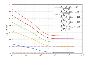
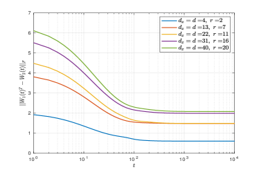
In the first set of experiments, we consider a general case of the balanced initial conditions, precisely $W_{j+1}^{T}(0)W_{j+1}(0)=W_{j}(0)W_{j}^{T}(0),\ j=1,\ldots,N-1,$ where condition (37) of Conjecture 41 is satisfied. The dimensions of the $W_{j}$ and their initializations are as follows. Recall, $W_{j}\in\mathbb{R}^{d_{j}\times d_{j-1}}$ for $j=1,\ldots,N$ where $d_{N}=d_{0}=d_{x}=d$ and $d_{1}=r$ is the rank of $W=W_{N}\cdots W_{1}$. We randomly generate $d_{j}\times d_{j}$ orthogonal matrices $V_{j}$ and then form $W_{j}(0)=V_{j}I_{d_{j}d_{1}}U_{j-1}^{T}$ for $j=1,\ldots,N$, where $U_{j}\in\mathbb{R}^{d_{j}\times d_{1}}$ is composed of the $d_{1}$ columns of $V_{j}$, and $I_{ab}$ is the (rectangular) $a\times b$ identity matrix. For all the values of $N$ and the different ranks of $W$ considered, Figure 1 shows that the limit of $W(t)$ as $t\rightarrow\infty$ is $U_{r}U_{r}^{T}$, where the columns of $U_{r}$ are $r$ eigenvectors of $XX^{T}$ corresponding to the largest $r$ eigenvalues of $XX^{T}$. This agrees with the theoretical results obtained for the autoencoder setting.

Figure 1. Convergence of solutions for the general balanced case. Error between $W(t)$ and $U_{r}U_{r}^{T}$ for different $r$ and $d$ values. Top left panel: $N=2$; top right panel: $N=5$; bottom left panel: $N=10$; bottom right panel: $N=20$.

Figure 2. Convergence of solutions for the general balanced case. Errors between $X$ and $W(t)X$ for different $r$ and $d$ values. Left panel: $N=2$; right panel: $N=20$.

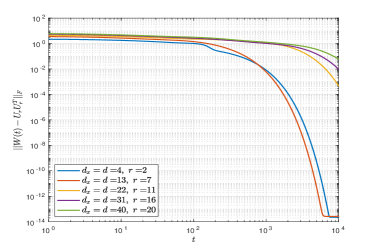
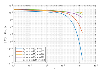
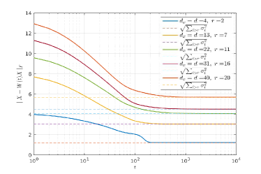
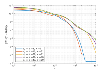
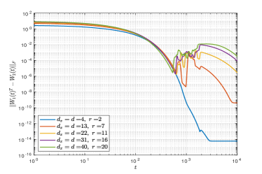
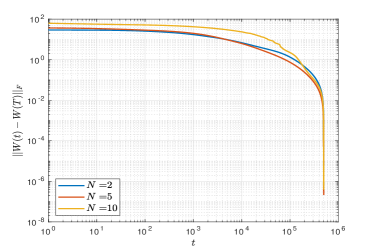
In addition, when $W(t)$ converges to $U_{r}U_{r}^{T}$ then $\|X-W(t)X\|_{F}$ converges to $\sqrt{\sum_{i>r}\sigma_{i}^{2}}$. This is also tested and confirmed for $N=2,5,10,20$, but for the purpose of saving space we show results for $N=2$ and $N=20$ in Figure 2. This depicts convergence of the functional $L^{1}(W(t))$ to the optimal error, which is the square-root of the sum of the tail eigenvalues of $XX^{T}$ of order greater than $r$. Moreover, in the autoencoder setting when $N=2$ we showed in Lemma 46 that the optimal solutions are $W_{2}=W_{1}^{T}$. This is also confirmed in the numerics as can be seen in the left panel plot of Figure 3.

Figure 3. Difference between $W_{1}(t)$ and $W_{2}(t)^{T}$ in the $N=2$ settings, for left panel: general balanced case; right panel: special balanced case.

Figure 4. In the special balanced case, left panel: norm of $W(t)$; right panel: errors between $W(t)$ and $U_{r}U_{r}^{T}$ for different $r$ and $d$ values.

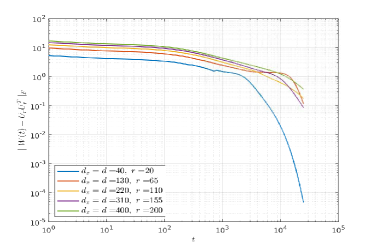
In the second set of experiments, we attempt to test Conjecture 41 by constructing pathological examples, where we have balanced initial conditions, but $W(0)$ violates condition (37) of Conjecture 41. Precisely, in the case $N=2$ we take $W_{1}(0)=V_{r}^{T}$ and $W_{2}(0)=-V_{r}$, where the columns of $V_{r}$ are the top $r$ eigenvectors of $XX^{T}$. Such $W(0)$ clearly violates the condition of the conjecture $u_{i}^{T}W(0)u_{i}>0$ for all $i\in[r]$.

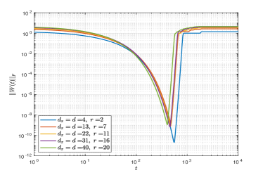
The hypothesis is that in such a setting the solution will not converge to the optimal solution proposed in Conjecture 41. Remark 42 showed that in such a case the solution should converge to $0$, that is $\lim_{t\rightarrow\infty}W(t)=0$. This can be seen in the left panel plot of Figure 4. The dip in the left panel shows that $W(t)$ is approaching zero in a first phase. However, probably due to numerical errors the flow escapes the equilibrium point at zero. In fact, zero is an unstable point (a strict saddle point), so that, numerically, the flow will hardly converge to zero. The right panel plot of Figure 4 shows very slow convergence to $U_{r}U_{r}^{T}$. Moreover, the limiting solutions (despite slow convergence) satisfy $W_{2}=W_{1}^{T}$ as shown in the right plot of Figure 3.

7.1.2. Non-balanced initial conditions

For $W_{j}(0)$, $j=1,\ldots,N$, we randomly generate Gaussian matrices. The two plots in Figure 5 and the left panel plot of Figure 6 show that $W(t)$ converges to $U_{r}U_{r}^{T}$. As in the balanced case we can confirm that $\|X-W(t)X\|_{F}$ converges to $\sqrt{\sum_{i>r}\sigma_{i}^{2}}$. On the other hand, for $N=2$ in this case we see that $W_{2}(t)$ does not converge to $W_{1}(t)^{T}$ in contrast to the balanced case, as can be seen in the right panel plot of Figure 6.

Figure 5. Non-balanced case convergence of solutions of the gradient flow. Errors between $W(t)$ and $U_{r}U_{r}^{T}$ for different $r$ and $d$ values for left panel: $N=2$, right panel: $N=5$.

Figure 6. Non-balanced case convergence. Left panel: Errors between $W(t)$ and $U_{r}U_{r}^{T}$ for different $r$ and $d$ values for $N=10$. Right panel: Errors between $W_{2}(t)$ and $W_{1}(t)^{T}$.

7.1.3. Convergence rates

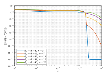
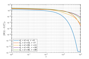
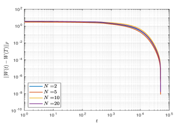
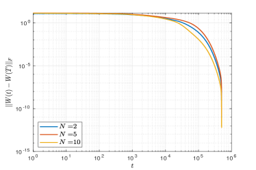
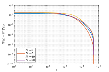
Here the data matrix $X\in\mathbb{R}^{d_{x}\times m}$ is generated with columns drawn i.i.d.from a Gaussian distribution, i.e., $x_{i}\sim\mathcal{N}(0,\sigma^{2}I_{d_{x}})$, where $\sigma=1/\sqrt{d_{x}}$. Random realization of $X$ with two different values for $d_{x}$ (as in above $m=3d$) and different $r$, the rank of $W(t)$, are used. For each fixed $d$, the dimensions $d_{j}$ of the $W_{j}\in\mathbb{R}^{d_{j}\times d_{j-1}}$ are selected using an arbitrarily chosen $r$ and setting $d_{j}=[r+(d-r)(j-1)/(N-1)]$ for $j=1,\ldots,N$. The value of $r$ is stated in the caption of the figures. The experiments show very rapid convergence of the solutions but also the dependence of the convergence rate on $N$, $d_{x}$, and $r$. We investigate this for different values of $N$, $d_{x}$ and $r$, in both the balanced and non-balanced cases. Convergence plots for the balanced initial conditions are shown in Figure 7, depicting smooth convergence. Similarly, we have convergence rates of the non-balanced case in Figure 8. These plots also show a slightly faster convergence for the balanced case than for the non-balanced case.

Figure 7. Convergence rates of solutions of the gradient flow in the autoencoder case with balanced initial conditions – errors between $W(t)$ and $W(T)$ for different $N$ values, where $T$ is the final time. Dimensions Left panel: $d_{x}=20$, $r=1$; Right panel: $d_{x}=200$, $r=10$.

Figure 8. Convergence rates of solutions of the gradient flow in the autoencoder case with non-balanced initial conditions – errors between $W(t)$ and $W(T)$ for different $N$ values, where $T$ is the final time. Dimensions Left panel: $d_{x}=20$, $r=1$; Right panel: $d_{x}=200$, $r=10$.

7.2. General supervised learning case

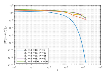
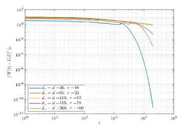
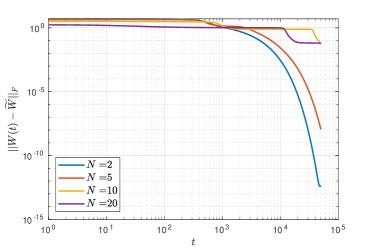
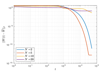
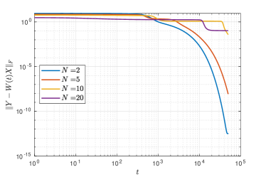
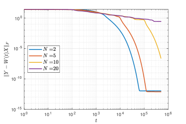
Experiments were also conducted to test the results in the general supervised learning setting to support theoretical results in Theorem 31 and Propositions 32 and 33. We show results for $N=2,5,10,20$, and two sets of values for $d_{x}$ and $r$ (rank of $W(t)$ and $\widetilde{W}$, the true parameters). The data matrix $X$ is generated as in the autoencoder case and $Y=\widetilde{W}X$, where $\widetilde{W}=\widetilde{W}_{N}\cdots\widetilde{W}_{1}$, with $\widetilde{W}_{j}\in\mathbb{R}^{d_{j}\times d_{j-1}}$ for $j=1,\ldots,N$ with $d_{N}=d_{0}=d_{x}=d$ and $d_{1}=r$ is the rank of $\widetilde{W}$. The entries of $\widetilde{W}_{j}$ are randomly generated independently from a Gaussian distribution with standard deviation $\sigma=1/\sqrt{d_{j}}$. The dimensions $d_{j}\times d_{j-1}$ of the $W_{j}$ for $j=1,\ldots,N$, are again selected respectively in an integer grid, i.e., $d_{j}=[r+(d_{x}-r)(j-1)/(N-1)]$, where $r$ is arbitrarily fixed. The initial conditions are generated as was done in the autoencoder case. We investigate the convergence rates for the balanced and non-balanced initial conditions of the gradient flows. The results of the experiments are plotted in Figures 9 and 10. In these plots $k$ is the rank of $Q\in\mathbb{R}^{d_{y}\times d_{x}}$ defined in (31), and $Q=U_{k}\Sigma_{k}V_{k}$ is the (reduced) singular value decomposition, i.e., $U_{k}\in\mathbb{R}^{d_{x}\times k}$ and $V_{k}\in\mathbb{R}^{d_{y}\times k}$ have orthonormal columns and $\Sigma_{k}\in\mathbb{R}^{k\times k}$ is a diagonal matrix containing the non-zero singular values of $Q$.

Figure 9. Convergence rates of solutions of the gradient flow of the general supervised learning problem depicted by convergence to $W$ in $(1)$ of Proposition 32 with balanced initial conditions for left panel: $d_{x}=20$, $r=2$; right panel: $d_{x}=200$, $r=20$.

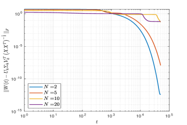
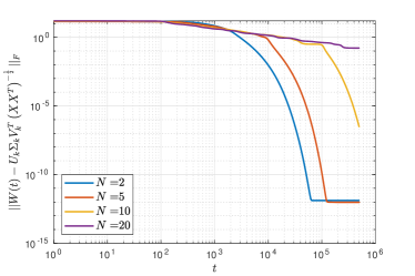
With balanced initial conditions the plots of Figure 9 show convergence rates of the flow to $W$ in $(1)$ of Proposition 32. With non-balanced initial conditions the plots of Figure 10 show convergence rates to $W$ in $(1)$ of Proposition 32. These results show rapid convergence of the flow and the dependence of the convergence rate on $N$, $r$ and $d_{x}$ with either balanced or non-balanced initial conditions. Note that $W$ in $(1)$ of Proposition 32 is the same as the true parameters $\widetilde{W}$. This can be seen by comparing the left panel plot of Figure 9 to the left panel plot of Figure 11 and the left panel plot of Figure 10 to the right panel plot of Figure 11.

Figure 10. Convergence rates of solutions of the gradient flow of the general supervised learning problem depicted by convergence to $W$ in $(1)$ of Proposition 32 with non-balanced initial conditions for left panel: $d_{x}=20$, $r=2$; right panel: $d_{x}=200$, $r=20$.

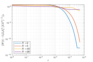
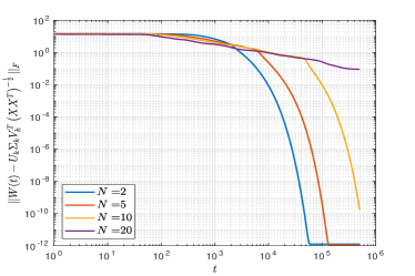
Convergence is slower for larger $N$, and it seems not to depend on the initial conditions, balanced or non-balanced, see the plots of Figures 9 and 10. Equivalently, this can be seen from the error of the supervised learning loss shown in the plots of Figure 12 for balanced initial conditions. There is much stronger dependence on $N$ in this setting than in the autoencoder setting.

Figure 11. Convergence to the true parameters $\widetilde{W}$ for ($d_{x}=20$, $r=2$) with left panel: balanced initial conditions; right panel: non-balanced initial conditions.

Figure 12. General supervised learning errors with balanced initial conditions for dimensions left panel: $d_{x}=20$, $r=2$; right panel: $d_{x}=200$, $r=20$.

7.3. Conclusion

To conclude the numerical section we summarise our results as follows. In the autoencoder case we confirmed that the solutions of the gradient flow converges to $U_{r}U_{r}^{T}$, while in the general supervised learning case we confirmed convergence of the flow to $W$ in $(1)$ of Proposition 32. Such convergence occurs with either balanced or non-balanced initial conditions albeit a slight faster convergence in the balanced than in the non-balanced. Secondly, in the autoencoder case we numerically confirmed the hypothesis of Conjecture 41 and that $W_{2}(t)=W_{1}(t)^{T}$ as claimed for $N=2$ with balanced initial conditions, which does not necessarily hold with non-balanced initial conditions. Moreover, in both the autoencoder and the general supervised learning setting we see that as the size ($N,d_{x},r$) of the problem instance increases the convergence rates decrease. In the autoencoder case we saw stronger dependence in $d_{x}$ and $r$ than in the general supervised learning case. On the other hand the dependence on $N$ seems to be stronger in the general supervised learning case than in the autoencoder case.

Appendix A Proof of Proposition 10

The proof is based on the next lemma, which follows from [8].

Lemma 43.

Let $A\in\mathbb{R}^{m\times m}$, $B\in\mathbb{R}^{n\times n}$, be positive definite matrices and $Y\in\mathbb{R}^{m\times n}$. Then, for $p\in\mathbb{N}$, $p\geq 2$, the solution $X\in\mathbb{R}^{m\times n}$ of the matrix equation

$$A^{p-1}X+A^{p-2}XB+\cdots+AXB^{p-2}+XB^{p-1}=Y$$ (40)

satisfies

$$X =\frac{\sin(\pi/p)}{\pi}\int_{0}^{\infty}(tI_{m}+A^{p})^{-1}Y(tI_{n}+B^{p})^{-1}t^{1/p}dt$$ (41)

$$=\frac{1}{p\Gamma(1-1/p)}\int_{0}^{\infty}\int_{0}^{t}e^{-sA^{p}}Ye^{-(t-s)B^{p}}ds\,t^{-(1+1/p)}dt.$$ (42)

Proof.

The first formula (41) is shown for $n=m$ in [8], for matrices with eigenvalues in $\{z\in\mathbb{C}:z\neq 0,-\pi/p<\arg z<\pi/p\}$. Positive definite matrices clearly have their eigenvalues in this set. Formula (41) extends to squares $A,B$ of possibly different dimensions $m,n$. In fact, [8] first proves (41) for $A=B$, see [8, eq. (8)] and then extends the solution by the “Berberian trick” which introduces the block matrices

$$\widetilde{A}=\left(\begin{matrix}A&0\\ 0&B\end{matrix}\right),\quad\widetilde{Y}=\left(\begin{matrix}0&Y\\ 0&0\end{matrix}\right),\quad\widetilde{X}=\left(\begin{matrix}X_{11}&X_{12}\\ X_{21}&X_{22}\end{matrix}\right).$$

If $\widetilde{X}$ solves $\sum_{i=1}^{p}\widetilde{A}^{p-i}\widetilde{X}\widetilde{A}^{i-1}=\widetilde{Y}$, then the submatrix $X=X_{12}$ solves (40) and one obtains (41). This argument works for general $m,n$ so that (41) holds under the conditions of the lemma.

In the case that $A=B$, [8, eq. (15)] implies (42). The general case of possibly different $A,B$ is then established again by the Berberian trick as above. ∎

Proof of Proposition 10.

We aim at applying Lemma 43 for the matrices $A=(WW^{T})^{1/N}$ and $B=(W^{T}W)^{1/N}$ in order to obtain a formula for $\bar{\mathcal{A}}_{W}^{-1}$. Unfortunately, in the rank deficient case, these matrices are only positive semi-definite and not positive definite. We will overcome this problem by using an approximation argument. For $u>0$, the matrices $(uI_{d_{y}}+WW^{T})^{1/N}$ and $(uI_{d_{x}}+W^{T}W)^{1/N}$ are positive definite and hence, the linear operator

$$\mathcal{A}_{W,u}:\mathbb{R}^{d_{y}\times d_{x}}\to\mathbb{R}^{d_{y}\times d_{x}},\quad\mathcal{A}_{W,u}(Z)=\sum_{j=1}^{N}(uI_{d_{y}}+WW^{T})^{\frac{N-j}{N}}Z(uI_{d_{x}}+W^{T}W)^{\frac{j-1}{N}}$$

is invertible by Lemma 43 with inverse $\mathcal{A}_{W,u}^{-1}:\mathbb{R}^{d_{y}\times d_{x}}\to\mathbb{R}^{d_{y}\times d_{x}}$,

$$\mathcal{A}_{W,u}^{-1}(Z)=\frac{\sin(\pi/N)}{\pi}\int_{0}^{\infty}\left((t+u)I_{d_{y}}+WW^{T}\right)^{-1}Z\left((t+u)I_{d_{x}}+W^{T}W\right)^{-1}t^{1/N}dt.$$ (43)

Furthermore, $\mathcal{A}_{W,u}$ maps $T_{W}(\mathcal{M}_{k})$ into $T_{W}(\mathcal{M}_{k})$ for all $u\geq 0$. Indeed, let $W=U\Sigma V^{T}$ be the full singular value decomposition of $W$ with $U$, $V$ being (square) orthogonal matrices and $\Sigma=\operatorname{diag}(\sigma_{1},\ldots,\sigma_{k},0,\ldots,0)$. If $Z=WA+BW\in T_{W}(\mathcal{M}_{k})$ then for $\alpha,\beta\geq 0$,

$$(uI_{d_{y}}+WW^{T})^{\alpha}Z(uI_{d_{x}}+W^{T}W)^{\beta}$$

$$\quad=U\operatorname{diag}((u+\sigma_{1}^{2})^{\alpha},\ldots,(u+\sigma_{k}^{2})^{\alpha},u^{\alpha},\ldots,u^{\alpha}))U^{T}U\Sigma V^{T}A(uI_{d_{x}}+W^{T}W)^{\beta}$$

$$\quad\quad+(uI_{d_{y}}+WW^{T})^{\alpha}BU\Sigma V^{T}V\operatorname{diag}((u+\sigma_{1}^{2})^{\beta},\ldots,(u+\sigma_{k}^{2})^{\beta},u^{\beta},\ldots,u^{\beta}))V^{T}$$

$$\quad=U\Sigma\operatorname{diag}((u+\sigma_{1}^{2})^{\alpha},\ldots,(u+\sigma_{k}^{2})^{\alpha},0,\ldots,0)V^{T}A(uI_{d_{x}}+W^{T}W)^{\beta}$$

$$\quad\quad+(uI_{d_{y}}+WW^{T})^{\alpha}BU\Sigma\operatorname{diag}((u+\sigma_{1}^{2})^{\beta},\ldots,(u+\sigma_{k}^{2})^{\beta},0,\ldots,0)V^{T}$$

$$\quad=WV\operatorname{diag}((u+\sigma_{1}^{2})^{\alpha},\ldots,(u+\sigma_{k}^{2})^{\alpha},0,\ldots,0)V^{T}A(uI_{d_{x}}+W^{T}W)^{\beta}$$

$$\quad\quad+(uI_{d_{y}}+WW^{T})^{\alpha}BU\operatorname{diag}((u+\sigma_{1}^{2})^{\beta},\ldots,(u+\sigma_{k}^{2})^{\beta},0,\ldots,0)U^{T}W.$$

The last expression is clearly an element of $T_{W}(\mathcal{M}_{k})$ and by the formula for $\mathcal{A}_{W,u}$ this implies that this operator maps the tangent space $T_{W}(\mathcal{M}_{k})$ into itself. Let us denote $\bar{\mathcal{A}}_{W,u}:T_{W}(\mathcal{M}_{k})\to T_{W}(\mathcal{M}_{k})$ the corresponding restriction and by $\bar{\mathcal{A}}^{-1}_{W,u}:T_{W}(\mathcal{M}_{k})\to T_{W}(\mathcal{M}_{k})$ the restriction of the inverse map to $T_{W}(\mathcal{M}_{k})$. Clearly, (43) still holds for the restriction $\bar{\mathcal{A}}^{-1}_{W,u}$. Lemma 8 implies that the restrictions $\bar{\mathcal{A}}_{W,u}$ and $\bar{\mathcal{A}}^{-1}_{W,u}$ are both well-defined also for $u=0$ with $\bar{\mathcal{A}}_{W,0}=\bar{\mathcal{A}}_{W}$ and $\bar{\mathcal{A}}^{-1}_{W,0}=\bar{\mathcal{A}}^{-1}_{W}$. Moreover, the map $u\mapsto\bar{\mathcal{A}}_{W,u}$ is continuous in $u\geq 0$ and, hence, also $u\mapsto\bar{\mathcal{A}}^{-1}_{W,u}$ is continuous in $u\geq 0$. We claim that also the right hand side of (43) with $Z\in T_{W}(\mathcal{M}_{k})$ is well-defined and continuous for all $u\geq 0$, which will give an inversion formula for $\bar{\mathcal{A}}^{-1}_{W}$ by setting $u=0$.

In order to show continuity of the right hand side of (43) in $u$, we investigate uniform integrability of the integrand for $Z\in T_{W}(\mathcal{M}_{k})$. By Lemma 7 we can write $Z=P_{W}(Z)=UP_{k}U^{T}Z(I_{d_{x}}-VP_{k}V^{T})+ZVP_{k}V^{T}$, where $P_{k}$ is the diagonal matrix from the lemma and $W=U\Sigma V^{T}$ is the (full) singular value decomposition of $W$. In particular, the matrix $\Sigma\in\mathbb{R}^{d_{y}\times d_{x}}$ has the singular values $\sigma_{1}\geq\ldots\geq\sigma_{k}>0$ on the diagonal, with all other entries equal to zero. For simplicity we write $E=I_{d_{x}}-VP_{k}V^{T}$. Denoting

$$\Lambda_{t,u} :=((t+u)I_{d_{y}}+\Sigma\Sigma^{T})^{-1}=\operatorname{diag}\left(\frac{1}{t+u+\sigma_{1}^{2}},\ldots,\frac{1}{t+u+\sigma_{k}^{2}},\frac{1}{t+u},\ldots,\frac{1}{t+u}\right)\in\mathbb{R}^{d_{y}\times d_{y}},$$

$$\widetilde{\Lambda}_{t,u} :=((t+u)I_{d_{x}}+\Sigma^{T}\Sigma)^{-1}=\operatorname{diag}\left(\frac{1}{t+u+\sigma_{1}^{2}},\ldots,\frac{1}{t+u+\sigma_{k}^{2}},\frac{1}{t+u},\ldots,\frac{1}{t+u}\right)\in\mathbb{R}^{d_{x}\times d_{x}},$$

$$K_{t,u} :=((t+u)I_{d_{y}}+\Sigma\Sigma^{T})^{-1}P_{k}=\operatorname{diag}\left(\frac{1}{t+u+\sigma_{1}^{2}},\ldots,\frac{1}{t+u+\sigma_{k}^{2}},0,\ldots,0\right)\in\mathbb{R}^{d_{y}\times d_{y}},$$

$$\widetilde{K}_{t,u} :=P_{k}((t+u)I_{d_{x}}+\Sigma^{T}\Sigma)^{-1}=\operatorname{diag}\left(\frac{1}{t+u+\sigma_{1}^{2}},\ldots,\frac{1}{t+u+\sigma_{k}^{2}},0,\ldots,0\right)\in\mathbb{R}^{d_{x}\times d_{x}}$$

we have

$$\left((t+u)I_{d_{y}}+WW^{T}\right)^{-1}Z\left((t+u)I_{d_{x}}+W^{T}W\right)^{-1} =UK_{t,u}U^{T}ZEV\widetilde{\Lambda}_{t,u}V^{T}+U\Lambda_{t,u}U^{T}ZV\widetilde{K}_{t,u}V^{T}.$$

Taking the spectral norm gives

$$\|\left((t+u)I_{d_{y}}+WW^{T}\right)^{-1}Z\left((t+u)I_{d_{x}}+W^{T}W\right)^{-1}\|_{2\to 2}\leq 2\|Z\|_{2\to 2}\sigma_{k}^{-2}(t+u)^{-1}\leq 2\|Z\|_{2\to 2}\sigma_{k}^{-2}t^{-1}.$$

This estimate will be good enough for $t\to 0$, for any $u>0$. For $t\to\infty$ we need a second estimate

$$\|\left((t+u)I_{d_{y}}+WW^{T}\right)^{-1}Z\left((t+u)I_{d_{x}}+W^{T}W\right)^{-1}\|_{2\to 2}$$

$$\quad\leq\|\left((t+u)I_{d_{y}}+WW^{T}\right)^{-1}\|_{2\to 2}\|Z\|_{2\to 2}\|\left((t+u)I_{d_{x}}+W^{T}W\right)^{-1}\|_{2\to 2}$$

$$\quad\leq\|Z\|_{2\to 2}(t+u)^{-2}\leq\|Z\|_{2\to 2}t^{-2},\vspace{-0.1cm}$$

which holds uniformly in $u>0$ and follows from the fact that $WW^{T}$ and $W^{T}W$ are positive semidefinite.

Altogether, for $Z\in T_{W}(\mathcal{M}_{k})$ the integrand in (43) satisfies

$$\|\left((t+u)I_{d_{y}}+WW^{T}\right)^{-1}Z\left((t+u)I_{d_{x}}+W^{T}W\right)^{-1}t^{1/N}\|_{2\to 2}\leq\|Z\|_{2\to 2}\min\{\sigma_{k}^{-2}t^{-1+1/N},t^{-2+1/N}\}.\vspace{-0.1cm}$$

The latter function is integrable over $t\in(0,\infty)$ since $N\geq 2$, and hence, for all $u\geq 0$, the integrand in (43) is uniformly dominated by an integrable function. By Lebesgue’s dominated convergence theorem and continuity of $u\mapsto\left((t+u)I_{d_{y}}+WW^{T}\right)^{-1}Z\left((t+u)I_{d_{x}}+W^{T}W\right)^{-1}t^{1/N}$ for all $t\in(0,\infty)$, the function $u\mapsto\bar{\mathcal{A}}_{W,u}^{-1}(Z)$ is continuous for all $Z\in T_{W}(\mathcal{M}_{k})$. Altogether, we showed that

$$\bar{\mathcal{A}}_{W}^{-1}(Z)=\frac{\sin(\pi/N)}{\pi}\int_{0}^{\infty}\left(tI_{d_{y}}+WW^{T}\right)^{-1}Z\left(tI_{d_{x}}+W^{T}W\right)^{-1}t^{1/N}dt,\quad Z\in T_{W}(\mathcal{M}_{k}),\vspace{-0.2cm}$$

and this implies (19).

A similar argument based on (42) proves (20). In the case $N=2$, it can be shown as in [7, Theorem VII.2.3] and with the approximation argument above that

$$\bar{\mathcal{A}}_{W}^{-1}(Z)=\int_{0}^{\infty}e^{-t(WW^{T})^{\frac{1}{2}}}Ze^{-t(W^{T}W)^{\frac{1}{2}}}\,dt,\vspace{-0.2cm}$$

which implies (21). ∎

Appendix B Proof of Proposition 11

Given a system $\{\gamma_{1},\ldots,\gamma_{n}\}$ of sufficiently smooth local coordinates on $\mathcal{M}_{k}$, where $n$ is the dimension of $\mathcal{M}_{k}$, the vectors $\xi_{j}(W):=\frac{\partial}{\partial\gamma_{j}}(W)$, $j=1,\ldots,n$, form a basis of the tangent space $T_{W}(\mathcal{M}_{k})$. We need to show that the maps

$$W\mapsto F_{i,j}(W):=g_{W}\left(\xi_{i}(W),\xi_{j}(W)\right)$$

are continuously differentiable for all $i,j$. Note that the vector fields $\xi_{j}(W)$ are smooth in $W$. We consider the representation (19) and introduce the functions

$$K_{i,j,t}(W):=\operatorname{tr}\left((t+WW^{T})^{-1}\xi_{i}(W)(t+W^{T}W)^{-1}\xi_{j}^{T}(W)\right),$$

where we write $(t+WW^{T})$ for $(tI_{d_{y}}+WW^{T})$ and likewise $(t+W^{T}W)=(tI_{d_{x}}+W^{T}W)$. For a function $f$ we denote the differential of $f$ at $A$ applied to $Y$ by $Df(A)[Y]$. Denoting $\phi_{t}(W)=(t+WW^{T})^{-1}$ and $\psi_{t}(W)=(t+W^{T}W)^{-1}$ the product rule gives, for $W\in\mathcal{M}_{k}$ and $Y\in T_{W}(\mathcal{M}_{k})$,

$$DK_{i,j,t}(W)[Y] =\operatorname{tr}(D\phi_{t}(W)[Y]\xi_{i}(W)\psi_{t}(W)\xi_{j}^{T}(W))+\operatorname{tr}(\phi_{t}(W)D\xi_{i}(W)[Y]\psi_{t}(W)\xi_{j}^{T}(W))$$ (44)

$$+\operatorname{tr}(\phi_{t}(W)\xi_{i}(W)D\psi_{t}(W)[Y]\xi_{j}^{T}(W))+\operatorname{tr}(\phi_{t}(W)\xi_{i}(W)\psi_{t}(W)D\xi_{j}^{T}(W)[Y]).$$ (45)

The differential of the function $\phi(A)=A^{-1}$ satisfies $D\phi(A)[Y]=-A^{-1}YA^{-1}$ so that

$$D\phi_{t}(W)[Y] =-(t+WW^{T})^{-1}(WY^{T}+YW^{T})(t+WW^{T})^{-1},$$

$$D\psi_{t}(W)[Y] =-(t+W^{T}W)^{-1}(W^{T}Y+Y^{T}W)(t+W^{T}W)^{-1}.$$

Let $W=U\Sigma V^{T}$ be the (full) singular value decomposition of $W$, i.e., $U\in\mathbb{R}^{d_{y}\times d_{y}}$, $V\in\mathbb{R}^{d_{x}\times d_{x}}$ with $U^{T}U=I_{d_{y}}$, $V^{T}V=I_{d_{x}}$ and $\Sigma=\operatorname{diag}(\sigma_{1},\ldots,\sigma_{k},0,\ldots,0)\in\mathbb{R}^{d_{y}\times d_{x}}$ with $\sigma_{1}\geq\cdots\geq\sigma_{k}>0$. The first term on the right hand side of (44) satisfies

$$\operatorname{tr}((D\phi_{t}(W)[Y]\xi_{i}(W)\psi_{t}(W)\xi_{j}^{T}(W))$$

$$=-\operatorname{tr}\left((t+WW^{T})^{-1}(WY^{T}+YW^{T})(t+WW^{T})^{-1}\xi_{i}(W)(t+W^{T}W)^{-1}\xi_{j}^{T}(W)\right).$$

Note that $(t+WW^{T})^{-1}(WY^{T}+YW^{T})(t+WW^{T})^{-1}=Q+Q^{T}$ with

$$Q=(t+WW^{T})^{-1}WY^{T}(t+WW^{T})^{-1}$$

$$=U\operatorname{diag}\left(\frac{1}{t+\sigma_{1}^{2}},\ldots,\frac{1}{t+\sigma_{k}^{2}},\frac{1}{t},\ldots,\frac{1}{t}\right)U^{T}(U\Sigma V^{T}Y^{T})U\operatorname{diag}\left(\frac{1}{t+\sigma_{1}^{2}},\ldots,\frac{1}{t+\sigma_{k}^{2}},\frac{1}{t},\ldots,\frac{1}{t}\right)U^{T}$$

$$=U\operatorname{diag}\left(\frac{\sigma_{1}}{t+\sigma_{1}^{2}},\ldots,\frac{\sigma_{k}}{t+\sigma_{k}^{2}},0,\ldots,0\right)V^{T}Y^{T}U\operatorname{diag}\left(\frac{1}{t+\sigma_{1}^{2}},\ldots,\frac{1}{t+\sigma_{k}^{2}},\frac{1}{t},\ldots,\frac{1}{t}\right)U^{T}.$$

By Lemma 7 it holds

$$\xi_{i}(W)=P_{W}(\xi_{i}(W))=UP_{k}U^{T}\xi_{i}(W)(I_{d_{x}}-VP_{k}V^{T})+\xi_{i}(W)VP_{k}V^{T}=\zeta^{1}_{i}(W)+\zeta^{2}_{i}(W).$$ (46)

where $P_{k}=\operatorname{diag}(1,\ldots,1,0,\ldots,0)$ (with $k$ ones on the diagonal), $\zeta^{1}_{i}(W)=UP_{k}U^{T}\xi_{i}(W)(I_{d_{x}}-VP_{k}V^{T})$ and $\zeta^{2}_{i}(W)=\xi_{i}(W)VP_{k}V^{T}$. Note that also $U$ and $V$ are functions of $W$, which may be non-unique, but in this case, we just fix one choice. Then we have

$$\xi_{i}(W)(t+W^{T}W)^{-1}\xi_{j}^{T}(W) =\overbrace{\zeta^{1}_{i}(W)(t+W^{T}W)^{-1}(\zeta^{1}_{j}(W))^{T}}^{=:E_{1}}+\overbrace{\zeta^{1}_{i}(W)(t+W^{T}W)^{-1}(\zeta^{2}_{j}(W))^{T}}^{=:E_{2}}$$

$$+\underbrace{\zeta^{2}_{i}(W)(t+W^{T}W)^{-1}(\zeta^{1}_{j}(W))^{T}}_{=:E_{3}}+\underbrace{\zeta^{2}_{i}(W)(t+W^{T}W)^{-1}(\zeta^{2}_{j}(W))^{T}}_{=:E_{4}}.$$

Using cyclicity of the trace, we obtain

$$\operatorname{tr}(QE_{1}) =\operatorname{tr}\left(\operatorname{diag}\left(\frac{\sigma_{1}}{t+\sigma_{1}^{2}},\ldots,\frac{\sigma_{k}}{t+\sigma_{k}^{2}},0,\ldots,0\right)V^{T}Y^{T}U\operatorname{diag}\left(\frac{1}{t+\sigma_{1}^{2}},\ldots,\frac{1}{t+\sigma_{k}^{2}},0,\ldots,0\right)\right.$$

$$\phantom{\operatorname{tr}(}\left.\times U^{T}\xi_{i}(W)(I_{d_{x}}-VP_{k}V^{T})V\operatorname{diag}\left(\frac{1}{t+\sigma_{1}^{2}},\ldots,\frac{1}{t+\sigma_{k}^{2}},\frac{1}{t},\ldots,\frac{1}{t}\right)V^{T}(I_{d_{x}}-VP_{k}V^{T})\xi_{j}^{T}(W)U\right),$$

$$\operatorname{tr}(QE_{2}) =\operatorname{tr}\left(\operatorname{diag}\left(\frac{\sigma_{1}}{t+\sigma_{1}^{2}},\ldots,\frac{\sigma_{k}}{t+\sigma_{k}^{2}},0,\ldots,0\right)V^{T}Y^{T}U\operatorname{diag}\left(\frac{1}{t+\sigma_{1}^{2}},\ldots,\frac{1}{t+\sigma_{k}^{2}},0,\ldots,0\right)\right.$$

$$\phantom{\operatorname{tr}(}\left.\times U^{T}\xi_{i}(W)(I_{d_{x}}-VP_{k}V^{T})V\operatorname{diag}\left(\frac{1}{t+\sigma_{1}^{2}},\ldots,\frac{1}{t+\sigma_{k}^{2}},0,\ldots,0\right)V^{T}\xi_{j}^{T}(W)U\right),$$

$$\operatorname{tr}(QE_{3}) =\operatorname{tr}\left(\operatorname{diag}\left(\frac{\sigma_{1}}{t+\sigma_{1}^{2}},\ldots,\frac{\sigma_{k}}{t+\sigma_{k}^{2}},0,\ldots,0\right)V^{T}Y^{T}U\operatorname{diag}\left(\frac{1}{t+\sigma_{1}^{2}},\ldots,\frac{1}{t+\sigma_{k}^{2}},\frac{1}{t},\ldots,\frac{1}{t}\right)\right.$$

$$\phantom{\operatorname{tr}(}\left.\times U^{T}\xi_{i}(W)V\operatorname{diag}\left(\frac{1}{t+\sigma_{1}^{2}},\ldots,\frac{1}{t+\sigma_{k}^{2}},0,\ldots,0\right)V^{T}(I_{d_{x}}-VP_{k}V^{T})\xi_{j}^{T}(W)U\right),$$

$$\operatorname{tr}(QE_{4}) =\operatorname{tr}\left(\operatorname{diag}\left(\frac{\sigma_{1}}{t+\sigma_{1}^{2}},\ldots,\frac{\sigma_{k}}{t+\sigma_{k}^{2}},0,\ldots,0\right)V^{T}Y^{T}U\operatorname{diag}\left(\frac{1}{t+\sigma_{1}^{2}},\ldots,\frac{1}{t+\sigma_{k}^{2}},\frac{1}{t},\ldots,\frac{1}{t}\right)\right.$$

$$\phantom{\operatorname{tr}(}\left.\times U^{T}\xi_{i}(W)V\operatorname{diag}\left(\frac{1}{t+\sigma_{1}^{2}},\ldots,\frac{1}{t+\sigma_{k}^{2}},0,\ldots,0\right)V^{T}\xi_{j}^{T}(W)U\right).$$

Note that $1/(t+\sigma_{i}^{2})\leq\min\{1/t,1/\sigma_{i}^{2}\}$ for all $t>0$. Using Cauchy-Schwarz inequality for the Frobenius inner product, the fact that $\|AB\|_{F}\leq\|A\|_{2\to 2}\|B\|_{F}$, and unitarity of $U$ and $V$, we obtain

$$|\operatorname{tr}(QE_{\ell})|\leq\|Y\|_{F}\|\xi_{i}(W)\|_{F}\|\xi_{j}(W)\|_{F}\sigma_{k}^{-3}t^{-1},\quad\ell=1,2,3,4.$$

By continuity of $\xi_{i}$ and $\xi_{j}$, it follows that there exists a neighborhood $\mathcal{U}\subset\mathcal{M}_{k}$ around a fixed $W_{0}\in\mathcal{M}_{k}$ (in which $\sigma_{k}(W)\geq c>0$ for some $c>0$ and all $W\in\mathcal{U}$) and a constant $C>0$ (depending only on the neighborhood) such that

$$|\operatorname{tr}(Q\xi_{i}(W)(t+W^{T}W)^{-1}\xi_{j}^{T}(W))|\leq C\|Y\|_{F}t^{-1}\quad\mbox{ for all }t>0\mbox{ and }W\in\mathcal{U}.$$

In the same way, one shows the above inequality for $Q$ replaced by $Q^{T}$ and hence

$$|\operatorname{tr}((D\phi_{t}(W)[Y]\xi_{i}(W)\psi_{t}(W)\xi_{j}^{T}(W))|\leq 2C\|Y\|_{F}t^{-1}\quad\mbox{ for all }t>0\mbox{ and }W\in\mathcal{U}.$$

Moreover, by the Cauchy-Schwarz inequality for the Frobenius inner product and since $WW^{T}$ as well as $W^{T}W$ are positive semidefinite, it holds

$$|\operatorname{tr}((D\phi_{t}(W)[Y]\xi_{i}(W)\psi_{t}(W)\xi_{j}^{T}(W))|$$

$$\quad\leq\|(t+WW^{T})^{-1}(WY^{T}+YW^{T})(t+WW^{T})^{-1}\|_{F}\|\xi_{i}(W)(t+W^{T}W)^{-1}\xi_{j}^{T}(W)\|_{F}$$

$$\quad\leq\|(t+WW^{T})^{-1}\|_{2\to 2}^{2}\|(t+W^{T}W)^{-1}\|_{2\to 2}\|WY^{T}+YW^{T}\|_{F}\|\xi_{i}(W)\|_{F}\|\xi_{j}(W)\|_{F}$$

$$\quad\leq 2t^{-3}\|WY^{T}\|_{F}\|\xi_{i}(W)\|_{F}\|\xi_{j}(W)\|_{F}.$$ (47)

Altogether, it holds, for a suitable constant $C_{1}>0$,

$$|\operatorname{tr}((D\phi_{t}(W)[Y]\xi_{i}(W)\psi_{t}(W)\xi_{j}^{T}(W))|\leq C_{1}\|Y\|_{F}\min\{t^{-1},t^{-3}\}\quad\mbox{ for all }t>0\mbox{ and }W\in\mathcal{U}.$$

Let us now consider the second term on the right hand side of (44). As in (47), we obtain

$$|\operatorname{tr}(\phi_{t}(W)D\xi_{i}(W)[Y]\psi_{t}(W)\xi_{j}^{T}(W))|\leq t^{-2}\|D\xi_{i}(W)[Y]\|_{F}\|\xi_{j}^{T}(W)\|_{F}.$$

By Lemma 7 we can write $\xi_{j}(W)=P_{W}(\xi_{j}(W))=\zeta^{1}_{j}(W)+\zeta^{2}_{j}(W)$ with $\zeta^{1}_{j}(W)=UP_{k}U^{T}\xi_{j}(W)(I_{d_{x}}-VP_{k}V^{T})$ and $\zeta^{2}_{j}(W)=\xi_{j}(W)VP_{k}V^{T}$ as in (46). With $E=I_{d_{x}}-VP_{k}V^{T}$ this gives

$$\operatorname{tr}(\phi_{t}(W)D\xi_{i}(W)[Y]\psi_{t}(W)\xi_{j}^{T}(W))$$

$$=\operatorname{tr}\left((t+WW^{T})^{-1}D\xi_{i}(W)[Y](t+W^{T}W)^{-1}(\zeta^{1}_{j}(W)+\zeta^{2}_{j}(W))^{T}\right)$$

$$=\operatorname{tr}\left(\operatorname{diag}\left(\frac{1}{t+\sigma_{1}^{2}},\ldots,\frac{1}{t+\sigma_{k}^{2}},0,\ldots,0\right)U^{T}D\xi_{i}(W)[Y]V\operatorname{diag}\left(\frac{1}{t+\sigma_{1}^{2}},\ldots,\frac{1}{t+\sigma_{k}^{2}},\frac{1}{t},\ldots,\frac{1}{t}\right)V^{T}E\xi_{j}^{T}(W)U\right)$$

$$+\operatorname{tr}\left(\operatorname{diag}\left(\frac{1}{t+\sigma_{1}^{2}},\ldots,\frac{1}{t+\sigma_{k}^{2}},\frac{1}{t},\ldots,\frac{1}{t}\right)U^{T}D\xi_{i}(W)[Y]V\operatorname{diag}\left(\frac{1}{t+\sigma_{1}^{2}},\ldots,\frac{1}{t+\sigma_{k}^{2}},0,\ldots,0\right)V^{T}\xi_{j}^{T}(W)U\right).$$

By the Cauchy-Schwarz inequality for the Frobenius inner product it follows that

$$|\operatorname{tr}(\phi_{t}(W)D\xi_{i}(W)[Y]\psi_{t}(W)\xi_{j}^{T}(W))|\leq 2\|D\xi_{i}(W)[Y]\|_{F}\|\xi_{j}(W)\|_{F}\sigma_{k}^{-2}t^{-1}.$$

Since the $\xi_{i}$ are continuously differentiable there exists $C_{2}>0$ such that

$$|\operatorname{tr}(\phi_{t}(W)D\xi_{i}(W)[Y]\psi_{t}(W)\xi_{j}^{T}(W))|\leq C_{2}\|Y\|_{F}\min\{t^{-1},t^{-2}\}\quad\mbox{ for all }t>0\mbox{ and }W\in\mathcal{U}.$$

The terms in (45) can be bounded in the same way as the ones in (44), hence

$$|DK_{i,j,t}(W)[Y]|\leq C^{\prime}\|Y\|_{F}\min\{t^{-1},t^{-2}\}\quad\mbox{ for all }t>0\mbox{ and }W\in\mathcal{U}.$$

It follows that $\int_{0}^{\infty}|DK_{i,j,t}(W)[Y]|t^{1/N}dt$ exists and is uniformly bounded in $W\in\mathcal{U}$. By Lebesgue’s dominated convergence theorem, it follows that we can interchange integration and differentiation, and hence, all directional derivatives of $F_{i,j}$ at $W$ in the direction of $Y$ exist and are continuous since $DK_{i,j,t}(W)[Y]$ is continuous in $W$ for all $Y\in T_{W}(\mathcal{M}_{k})$. Hence, by (19), $F_{i,j}$ is (totally) continuously differentiable for all $i,j$ with

$$DF_{i,j}(W)[Y]=\frac{\sin(\pi/N)}{\pi}\int_{0}^{\infty}DK_{i,j,t}(W)[Y]t^{1/N}dt.$$

Hence, the metric is of class $C^{1}$ as claimed.

Appendix C Some results on flows on manifolds

Here we summarize some notions and results on flows on manifolds that can be found in [15, Chapter IV,§2] to which we also refer for more details.

Let $p\geq 2$ be an integer or $p=\infty$, let $\mathcal{M}$ be a (finite dimensional) $C^{p}$-manifold and let $\xi$ be a vector field of class $C^{p-1}$ on $\mathcal{M}$. An integral curve for $\xi$ with initial condition $x_{0}\in\mathcal{M}$ is a $C^{p-1}$-curve

$$\gamma:J\to\mathcal{M},$$

where $J$ is an open intervall containing $0$ such that

$$\dot{\gamma}(t)=\xi(\gamma(t))\ \ \forall t\in J\ \text{ and }\gamma(0)=x_{0}.$$

Theorem 44 (Theorem 2.1 in Chapter IV,§2 in [15]).

If $\gamma_{1}:J_{1}\to\mathcal{M}$ and $\gamma_{2}:J_{2}\to\mathcal{M}$ are integral curves for $\xi$ with the same initial condition then $\gamma_{1}=\gamma_{2}$ on $J_{1}\cap J_{2}$.

Let $D(\xi)\subseteq\mathbb{R}\times\mathcal{M}$ be the set of all pairs $(t,x_{0})$ such that for any $x_{0}\in\mathcal{M}$ the set

$$J(x_{0}):=\{t\in\mathbb{R}\ |\ (t,x_{0})\in D(\xi)\}$$

is the maximal open existence interval of an integral curve for $\xi$ with initial condition $x_{0}$. For any $x_{0}\in\mathcal{M}$, this interval is non-empty (locally one can argue as in the case $\mathcal{M}=\mathbb{R}^{n}$).

A global flow for $\xi$ is a mapping

$$\alpha:D(\xi)\to\mathcal{M}$$

such that for all $x_{0}\in\mathcal{M}$ the map $t\mapsto\alpha(t,x_{0})$ for $t\in J(x_{0})$ is an integral curve for $\xi$ with initial condition $x_{0}$, i.e. $\alpha(0,x_{0})=x_{0}$ and $\dot{\alpha}(t,x_{0})=\xi(\alpha(t,x_{0}))$ for any $t\in J(x_{0})$. Note that by Theorem 44 there is only one such mapping $\alpha$. For $t\in\mathbb{R}$ let

$$D_{t}(\xi):=\{x\in\mathcal{M}\ |\ (t,x)\in D(\xi)\}$$

and define the map $\alpha_{t}\colon D_{t}(\xi)\to\mathcal{M}$ by $\alpha_{t}(x)=\alpha(t,x)$.

Theorem 45 (Theorems 2.6 and 2.9 in Chapter IV,§2 in [15]).

1. The set $D(\xi)$ is open in $\mathbb{R}\times\mathcal{M}$ and $\alpha$ is a $C^{p-1}$-morphism.

2. For any $t\in\mathbb{R}$, the set $D_{t}(\xi)$ is open in $\mathcal{M}$ and (for $D_{t}(\xi)$ non-empty) $\alpha_{t}$ defines a diffeomorphism of $D_{t}(\xi)$ onto an open subset of $\mathcal{M}$ (namely $\alpha_{t}(D_{t}(\xi))=D_{-t}(\xi))$ and $\alpha_{t}^{-1}=\alpha_{-t}$).

Appendix D The non-symmetric autoencoder case for $N=2$

Here we consider the optimization problem (3) with $N=2$ and the additional constraint that $Y=X$, but we do not assume that $W_{2}=W_{1}^{T}$. We also assume balanced starting conditions, i.e., $W_{2}(0)^{T}W_{2}(0)=W_{1}(0)W_{1}(0)^{T}$. In this special case, we can use a more direct approach than in Section 6 to establish some additional explicit statements below.

We write again $d$ for $d_{x}=d_{y}$ and $r$ for $d_{1}$. The equations for the flow here are:

$$\begin{split}\dot{W_{1}}&=-W_{2}^{T}W_{2}W_{1}XX^{T}+W_{2}^{T}XX^{T},\\ \dot{W_{2}}&=-W_{2}W_{1}XX^{T}W_{1}^{T}+XX^{T}W_{1}^{T}.\end{split}$$ (48)

Next we analyze the equilibrium points of the flow (48) and of the product $W=W_{2}W_{1}$ again assuming balanced initial conditions. We begin by exploring the equilibrium points of the flow (48) by setting the expressions in (48) equal to zero:

$$\begin{split}-W_{2}^{T}W_{2}W_{1}XX^{T}+W_{2}^{T}XX^{T}&=0,\\ -W_{2}W_{1}XX^{T}W_{1}^{T}+XX^{T}W_{1}^{T}&=0.\end{split}$$ (49)

If $W_{2}\in\mathbb{R}^{d\times r}$ is the zero matrix then (since $XX^{T}$ has full rank) it follows that (49) is solved if and only if $W_{1}$ is the $r\times d$ zero-matrix, hence $W$ is the $d\times d$ zero-matrix. The following lemma characterizes the non-trivial solutions. (The second part of the lemma is a special case of Proposition 32 below.)

Lemma 46.

The balanced nonzero solutions (i.e. solutions with $W_{2}\neq 0$) of (49) are precisely the matrices of the form

$$W_{2}=UV^{T},\quad W_{1}=W_{2}^{T}=VU^{T},\quad W=W_{2}W_{1}=UU^{T},$$ (50)

where $U\in\mathbb{R}^{d\times k}$ for some $1\leq k\leq r$ and where the columns of $U$ are orthonormal eigenvectors of $XX^{T}$ and $V\in\mathbb{R}^{r\times k}$ has orthonormal columns.

In particular, the equilibrium points for $W=W_{2}W_{1}$ are precisely the matrices of the form

$$W=\sum_{j=1}^{k}u_{j}u_{j}^{T},$$ (51)

where $k\in\{1,\ldots,r\}$ and $u_{1},\ldots,u_{k}$ (the columns of $U$ above) are orthonormal eigenvectors of $XX^{T}$.

Remark 47.

Note that $W=0$ is also an equilibrium point of (48) which formally corresponds to taking $k=0$ in (51).

Proof.

Since $W_{2}\neq 0$, the rank $k$ of $W_{2}$ is at least $1$. The balancedness condition $W_{2}^{T}W_{2}=W_{1}W_{1}^{T}$ implies that $W_{1}$ and $W_{2}$ have the same singular values. Since $XX^{T}$ has full rank, the first equation of (49) yields $W_{2}^{T}=W_{2}^{T}W_{2}W_{1}$. Again due to balancedness, this shows that $W_{2}^{T}=W_{1}W_{1}^{T}W_{1}$. It follows that all positive singular values of $W_{1}$ and of $W_{2}$ are equal to $1$ and that $W_{2}=W_{1}^{T}$. The second equation of (49) thus gives the equation

$$(I_{d}-W_{2}W_{2}^{T})XX^{T}W_{2}=0.$$ (52)

(The equilibrium points of full rank $r$ could now be obtained using [23, Propositon 4.1] again, but we are interested in all solutions here.) Since the positive singular values of $W_{2}$ are all equal to $1$, it follows that we can write

$$W_{2}W_{2}^{T}=\sum_{i=1}^{k}u_{i}u_{i}^{T},$$

where the $u_{i}$ are orthonormal. We extend the system $u_{1},\ldots,u_{k}$ to an orthonormal basis $u_{1},\ldots,u_{d}$ of $\mathbb{R}^{d}$. From (52) we obtain $(I_{d}-W_{2}W_{2}^{T})XX^{T}W_{2}W_{2}^{T}=0$, hence $\sum_{j=k+1}^{d}u_{j}u_{j}^{T}XX^{T}\sum_{i=1}^{k}u_{i}u_{i}^{T}=0$ and consequently

$$\sum_{j=k+1}^{d}\sum_{i=1}^{k}(u_{j}^{T}XX^{T}u_{i})u_{j}u_{i}^{T}=0.$$

It follows that for all $j\in\{k+1,\ldots,d\}$ and for all $i\in\{1,\ldots,k\}$ we have $u_{j}^{T}XX^{T}u_{i}=0$. This in turn implies that $XX^{T}$ maps the span of $u_{1},\ldots,u_{k}$ into itself and also maps the span of $u_{k+1},\ldots,u_{d}$ into itself. This implies that we can choose $u_{1},\ldots,u_{d}$ as orthonormal eigenvectors of $XX^{T}$. Thus we can indeed write the (reduced) singular value decomposition of $W_{2}$ as $W_{2}=UV^{T}$, where the columns $u_{1},\ldots,u_{k}$ of $U$ are orthonormal eigenvectors of $XX^{T}$ and where $V$ is as in the statement of the lemma. Since $W_{1}=W_{2}^{T}$ and $W=W_{2}W_{1}$, it follows that $W_{1}=VU^{T}$ and $W=UU^{T}$ as claimed. Altogether, we have shown that the equations (50) are necessary for having a balanced solution of (49). One easily checks that $W_{1},W_{2}$ defined by (50) also satisfy (49), which shows sufficiency. This completes the proof. ∎

Corollary 48.

Consider a linear autoencoder with one hidden layer of size $r$ with balanced initial conditions and assume that $XX^{T}$ has eigenvalues $\lambda_{1}\geq\ldots\geq\lambda_{d}>0$ and corresponding orthonormal eigenvectors $u_{1},\ldots,u_{d}$.

1. The flow $W(t)$ always converges to an equilibrium point of the form $W=\sum_{j\in J_{W}}u_{j}u_{j}^{T},$ where $J_{W}$ is a (possibly empty) subset of $\{1,\ldots,d\}$ of at most $r$ elements.

2. The flow $W_{2}(t)$ converges to $UV^{T}=:W_{2}$, where the columns of $U$ are the $u_{j},j\in J_{W}$ and $V\in\mathbb{R}^{r\times k}$ has orthonormal columns ($k=|J_{W}|$) . Furthermore $W_{1}(t)$ converges to $W_{2}^{T}$.

3. If $L^{1}(W(0))<\frac{1}{2}\sum_{i=r,i\neq r+1}^{d}\lambda_{i}$ then $W(t)$ converges to the optimal equilibrium $W=\sum_{j=1}^{r}u_{j}u_{j}^{T}$.

4. If $\lambda_{r}>\lambda_{r+1}$, then there is an open neighbourhood of the optimal equilibrium point in which we have convergence of the flow $W(t)$ to the optimal equilibrium point.

Proof.

The first and the second point follow from Lemma 46 together with Theorem 5. (Note that if $(W_{1},W_{2})$ is an equilibrium point to which the flow converges then $W_{1},W_{2}$ are balanced since we assume that the flow has balanced initial conditions.) To prove the third point, note that the loss of an equilibrium point $W=\sum_{j\in J_{W}}u_{j}u_{j}^{T}$ is given by $L^{1}(W)=\frac{1}{2}\sum_{i\in K_{W}}\lambda_{i}$, where $K_{W}=\{1,\ldots,d\}\setminus J_{W}$. This sum is minimal for $J_{W}=\{1,\ldots,r\}$. Among the remaining possible $J_{W}$, the value of $L^{1}(W)$ is minimal for $J_{W}=\{1,\ldots,r+1\}\setminus\{r\}$, i.e., $K_{W}=\{r,\ldots,d\}\setminus\{r+1\}$. Since the value of $L^{1}(W(t))$ monotonically decreases as $t$ increases (as follows e.g. from equation (24)), the claim now follows from the first point. The last point follows from the third point. ∎

The following result is an analogue to Theorem 25.

Theorem 49.

If $k\leq r$ and $u_{1},\ldots,u_{k}$ are orthonormal eigenvectors of $XX^{T}$ which do not form a system of eigenvectors to the $r$ largest eigenvalues of $XX^{T}$ (in particular for $k<r$), in any neighborhood of the equilibrium point $W=\sum_{j=1}^{k}u_{j}u_{j}^{T}$ there is some $\widetilde{W}$ of rank at most $r$ for which $L^{1}(\widetilde{W})<L^{1}(W)$. In particular, the equilibrium in $W$ is non-stable.

Proof.

If $k<r$ and $W=\sum_{j=1}^{k}u_{j}u_{j}^{T}$ for orthonormal eigenvectors $u_{j}$ of $XX^{T}$ then for any additional eigenvector $u_{k+1}$ orthonormal to the $u_{j}$ and for any $\varepsilon>0$, we can choose $\widetilde{W}=W+\varepsilon u_{k+1}u_{k+1}^{T}$ to obtain $L^{1}(\widetilde{W})<L^{1}(W)$. Let now $k=r$. This case can be treated analogously to the proof of Theorem 25: let $u_{i}$ be one of the eigenvectors $u_{1},\ldots,u_{r}$ whose eigenvalue does not belong to the $r$ largest eigenvalues of $XX^{T}$. Let $v$ be an eigenvector of $XX^{T}$ of unit length which is orthogonal to the eigenvectors $u_{1},\ldots,u_{r}$ and whose eigenvalue belongs to the $r$ largest eigenvalues of $XX^{T}$. Now for any $\varepsilon\in[0,1]$ consider $u_{i}(\varepsilon):=\varepsilon v+\sqrt{1-\varepsilon^{2}}u_{i}$. Then $W(\varepsilon):=u_{i}(\varepsilon)u_{i}(\varepsilon)^{T}+\sum_{j=1,j\neq i}^{r}u_{j}u_{j}^{T}$ satisfies $L^{1}(W(\varepsilon))<L^{1}(W)$ for $\varepsilon\in(0,1]$. From this the claim follows. ∎

Remark 50.

With the notation

$$V=\begin{pmatrix}W_{1}^{T}\\ W_{2}\end{pmatrix}\in\mathbb{R}^{2d\times r}\text{ and }C=XX^{T}\in\mathbb{R}^{d\times d}$$

and assuming that $C$ has full rank, the flow (48) can be written as the following Riccati-type-like ODE.

$$\dot{V}=\left(I_{2d}+\begin{pmatrix}-C&0\\ 0&0\end{pmatrix}VV^{T}\begin{pmatrix}0&0\\ C^{-1}&0\end{pmatrix}+\begin{pmatrix}0&0\\ 0&-I_{d}\end{pmatrix}VV^{T}\begin{pmatrix}0&I_{d}\\ 0&0\end{pmatrix}\right)\begin{pmatrix}0&C\\ C&0\end{pmatrix}V.$$ (53)

References

- [1] P. A. Absil, R. Mahony, and B. Andrews. Convergence of the iterates of descent methods for analytic cost functions. SIAM J. Optim. 16(2), pp. 531-547, 2005.
- [2] P.-A. Absil, R. Mahony, and R. Sepulchre. Optimization Algorithms on Matrix Manifolds. Princeton University Press, 2008.
- [3] P.-A. Absil, I.V. Oseledets. Low-rank retractions: a survey and new results. Comput. Optim. Appl. 62: 5–29, 2015.
- [4] S. Arora, N. Cohen, N. Golowich, and W. Hu. A convergence analysis of gradient descent for deep linear neural networks, ICLR, 2019. (arXiv:1810.02281).
- [5] S. Arora, N. Cohen, and E. Hazan. On the optimization of deep networks: Implicit acceleration by overparameterization. Preprint arXiv:1802.06509, 2018.
- [6] A. Banyaga, D. Hurtubise. Lectures on Morse homology. Springer Science and Business Media, 2004.
- [7] R. Bhatia. Matrix Analysis, volume 169. Springer, 1997.
- [8] R. Bhatia, M. Uchiyama. The operator equation . Expo. Math. 27:251–255, 2009.
- [9] E. Carlen and J. Maas. An analog of the 2-Wasserstein metric in non-commutative probability under which the fermionic Fokker-Planck equation is gradient flow for the entropy. Comm. Math. Phys., 331, 2012.
- [10] Y. Chitour, Z. Liao, and R. Couillet. A geometric approach of gradient descent algorithms in neural networks. Preprint, arXiv:1811.03568, 2018.
- [11] I. Goodfellow, Y. Bengio, and A. Courville. Deep Learning. MIT Press, 2016. http://www.deeplearningbook.org.
- [12] U. Helmke and M. A. Shayman. Critical points of matrix least squares distance functions. Lin. Alg. Appl., 215:1–19, 1995.
- [13] K. Kawaguchi. Deep learning without poor local minima. Advances in Neural Information Processing Systems 29, pages 586–594, 2016.
- [14] K. Kurdyka, T. Mostowski, and A. Parusinski. Proof of the gradient conjecture of R. Thom. Ann. of Math. (2), 152, pp. 763–792, 2000.
- [15] S. Lang. Fundamentals of Differential Geometry. Springer, 1999.
- [16] J. D. Lee, I. Panageas, G. Piliouras, M. Simchowitz, M. I. Jordan, and B. Recht. First-order methods almost always avoid strict saddle points. Math. Program., 176(1):311–337, 2019.
- [17] S. Lojasiewicz. Sur les trajectoires du gradient d’une fonction analytique. Seminari di geometria, 1983:115–117, 1984.
- [18] K. P. Murphy. Machine learning: a probabilistic perspective. MIT Press, Cambridge, Mass. [u.a.], 2013.
- [19] F. Otto and M. Westdickenberg. Eulerian calculus for the contraction in the Wasserstein distance. SIAM J. Math. Analysis, 37:1227–1255, 2005.
- [20] M. Shub. Global Stability of Dynamical Systems. Springer, 1986.
- [21] L. Simon. Theorems on Regularity and Singularity of Energy Minimizing Maps. Birkhäuser, 1996.
- [22] M. Trager, K. Kohn, J. Bruna, Pure and spurious critical points: a geometric study of linear networks. Preprint arXiv:1910.01671, 2019.
- [23] W. Yan, U. Helmke, and J. B. Moore. Global analysis of Oja’s flow for neural networks. IEEE Trans. Neural Netw., 5(5):674–683, 1994.