Pulsar glitch activity as a state-dependent Poisson process: parameter estimation and epoch prediction

Abstract

Rotational glitches in some rotation-powered pulsars display power-law size and exponential waiting time distributions. These statistics are consistent with a state-dependent Poisson process, where the glitch rate is an increasing function of a global stress variable (e.g. crust-superfluid angular velocity lag), diverges at a threshold stress, increases smoothly while the star spins down, and decreases step-wise at each glitch. A minimal, seven-parameter, maximum likelihood model is calculated for PSR J1740$-$3015, PSR J0534$+$2200, and PSR J0631$+$1036, the three objects with the largest samples whose glitch activity is Poisson-like. The estimated parameters have theoretically reasonable values and contain useful information about the glitch microphysics. It is shown that the maximum likelihood, state-dependent Poisson model is a marginally (23–27 per cent) better post factum “predictor” of historical glitch epochs than a homogeneous Poisson process for PSR J1740$-$3015 and PSR J0631$+$1036 and a comparable predictor for PSR J0534$+$2200. Monte Carlo simulations imply that $\gtrsim 50$ glitches are needed to test reliably whether one model outperforms the other. It is predicted that the next glitch will occur at Modified Julian Date (MJD) $57784\pm 256.8$, $60713\pm 1935$, and $57406\pm 1444$ for the above three objects respectively. The analysis does not apply to quasiperiodic glitchers like PSR J0537$-$6910 and PSR J0835$-$4510, which are not described accurately by the state-dependent Poisson model in its original form.

1 Introduction

The secular, electromagnetic braking of some rotation-powered pulsars is interrupted by random, impulsive, spin-up events called glitches (Lyne & Graham-Smith, 2012). Two categories of glitch activity have been identified (Melatos et al., 2008; Espinoza et al., 2011; Onuchukwu & Chukwude, 2016; Howitt et al., 2018; Carlin & Melatos, 2019b; Fuentes et al., 2019): Poisson-like, in which the waiting time probability density function (PDF) is exponential, and the size PDF is a power law over $\lesssim 4\,{\rm dex}$; and quasiperiodic, where both the size and waiting time PDFs are approximately Gaussian and centered on characteristic values. Most glitching pulsars with statistically significant glitch samples fall into one of the categories above, although there is some cross-over. For example, PSR J0534$+$2200 is Poisson-like (Wong et al., 2001), PSR J0537$-$6910 is quasiperiodic (Middleditch et al., 2006; Ferdman et al., 2018), and PSR J1341$-$6220 appears to be a hybrid (Howitt et al., 2018) with log-normal characteristics (Fuentes et al., 2019). The physical origin of glitches remains unknown but is linked commonly to a combination of internal processes such as starquakes and superfluid vortex avalanches (Haskell & Melatos, 2015).

Glitches are stochastic, in the sense that the epochs and sizes of individual events are unpredictable. Among the $\gtrsim 200$ pulsars in which glitches have been recorded, only a handful offer exceptions to this rule. A tight, three-sigma correlation of $6.5\,{\rm days\,}\mu{\rm Hz}^{-1}$ is observed between sizes and forward waiting times in PSR J0537$-$6910, which can be exploited to predict the epoch of the next glitch to within $\pm 3$ days; see the ‘staircase plots’ in Fig. 8 in Middleditch et al. (2006) and Fig. 2 in Ferdman et al. (2018). An analogous three-sigma correlation is observed in PSR J1801$-$2304 (Melatos et al., 2018; Fuentes et al., 2019). Weaker correlations between sizes and forward waiting times can also be discerned in PSR J1341$-$6220 (Yuan et al., 2010; Melatos et al., 2018; Fuentes et al., 2019), PSR J0205$+$6449 (Melatos et al., 2018; Fuentes et al., 2019), and PSR J1645$-$0317 (Shabanova, 2009). However more data are needed to evaluate their power as an epoch prediction tool, and the events in PSR J1645$-$0317 are ‘slow’ glitches, whose rise times are resolved over $\sim 1\,{\rm yr}$. Beyond the above examples, no size-waiting-time correlations have been measured, which could be exploited for the purpose of epoch prediction, not even in quasiperiodic objects. Independently, in PSR J0835$-$4510, there is evidence that a glitch is triggered, when the transient impulse response to the previous glitch recovers fully, if one corrects for the quasiexponential post-glitch relaxation and the inter-glitch frequency second derivative (Akbal et al., 2017). This approach predicts glitch epochs in PSR J0835$-$4510 with an uncertainty of about $\pm 150\,{\rm days}$ and deserves to be tested against other pulsars, e.g. Yu et al. (2013). Second-frequency-derivative corrections can be related to the physics of nonlinear vortex creep (Alpar et al., 1984).

In this paper, we approach the challenge of epoch prediction by modeling glitch activity as a state-dependent Poisson process (Fulgenzi et al., 2017; Melatos et al., 2018; Carlin & Melatos, 2019b, a), in which the glitch rate is variable and depends instantaneously on the ‘stress’ in the system (elastic stress in the starquake picture, crust-superfluid differential rotation in the vortex avalanche picture). The model naturally predicts two categories of glitch activity (Fulgenzi et al., 2017; Carlin & Melatos, 2019b) and a paucity of size-waiting-time auto- and cross-correlations (Melatos et al., 2018; Carlin & Melatos, 2019a) in line with observations. It also allows us to reconstruct the stress history of a pulsar from the observed sequence of glitch sizes and epochs in terms of seven model parameters and hence derive a maximum likelihood estimate of the stress value today, which in turn predicts a Poisson waiting time to the next glitch. This prediction should be better than the unmodeled prediction based on the time-averaged rate inferred from the waiting time PDF, if the stress and hence the instantaneous rate vary from one glitch to the next (Fulgenzi et al., 2017; Melatos et al., 2018; Carlin et al., 2019).

The paper is structured as follows. The minimal version of the state-dependent Poisson model is reviewed briefly in §2, and a maximum likelihood estimator is constructed for the seven parameters which control the model’s behavior. Maximizing the likelihood is not trivial. Two numerical maximization techniques, particle swarm and nested sampling, are presented and tested for accuracy against synthetic data in §3. The seven model parameters are estimated for three objects with Poisson-like glitch activity in §4, namely PSR J1740$-$3015, PSR J0534$+$2200, and PSR J0631$+$1036. The physical significance of the best-fit parameters is discussed. Finally the maximum likelihood estimates in §4 are used to “predict” post factum the epochs of past glitches for the above three objects (as a validation test) and then to genuinely predict the epoch of the next, future glitch (with confidence intervals). The predictions are therefore directly falsifiable over time. Parameter estimation for other, Poisson-like glitchers with smaller samples is premature at this juncture. The minimal version of the state-dependent Poisson model introduced by Fulgenzi et al. (2017) does not describe accurately the glitch activity of quasiperiodic glitchers like PSR J0537$-$6910 and PSR J0835$-$4510, so the latter category of object is not analysed here.

2 State-dependent Poisson process

For various physical mechanisms, glitch activity is controlled in the mean-field approximation by a single, global, random variable, $X(t)$, which measures the spatially averaged crust-superfluid angular velocity lag (vortex avalanche picture) or the crustal elastic stress (starquake picture) as a function of time $t$. In between glitches, $X(t)$ increases secularly in response to the electromagnetic braking torque $N_{\rm em}$, with $\dot{X}\propto|N_{\rm em}|$. When a glitch occurs, $X$ decreases discontinuously by a random amount determined by the avalanche physics governing the glitch trigger, e.g. vortex unpinning (Warszawski & Melatos, 2011) or crust cracking (Chugunov & Horowitz, 2010). The combination of a slow, global driver, which adds stress, and local, stick-slip relaxation, which releases stress, is characteristic of systems that exhibit self-organized criticality (Jensen, 1998; Melatos et al., 2008).

In §2.1 and §2.2, we model the evolution of $X(t)$ in an idealized fashion as a state-dependent Poisson process (Daly & Porporato, 2007; Wheatland, 2008; Warszawski & Melatos, 2013; Fulgenzi et al., 2017; Carlin & Melatos, 2019b). We then construct a maximum likelihood estimator of the model’s seven control parameters from an observed sequence of glitch sizes and waiting times in §2.3. A state-dependent Poisson process occupies a well-defined place within the established taxonomy of stochastic processes. In a general sense, it is a marked renewal process: marked, because every event is tagged with auxiliary information (here, the glitch size) besides its epoch; and renewal, because it involves stochastically recurring events, whose waiting time distribution resets after every glitch. A state-dependent Poisson process may also be regarded as doubly stochastic, because the event rate itself is a random variable; it increases deterministically between glitches, but its starting value immediately after every glitch depends on the random, post-glitch value of $X$. A state-dependent Poisson process is more general than an inhomogeneous, Poisson process because it is marked, and because the rate is stochastic. It is also more general than a continuous-time jump Markov process, because the waiting time distribution depends on the whole time series $X(t)$ since the previous glitch, not just $X$ at the previous time step. (The glitch sizes constitute a jump Markov process when viewed in isolation.) The reader is referred to the textbooks by Kingman (1993) and Del Moral & Penev (2017) for a comprehensive classification of stochastic processes, including formal definitions of the terms above.

2.1 Equations of motion

It is convenient to write the equations of motion in dimensionless form in order to identify clearly the minimum set of irreducible parameters in the model. Let $X_{\rm c}$ be the critical crust-superfluid angular velocity lag, at which the Magnus force exceeds the vortex pinning force globally, and a glitch is certain to occur (Link & Epstein, 1991). (An analogous threshold is easy to define in the starquake picture, but we focus here on glitches triggered by vortex unpinning for the sake of definiteness.) Let $I_{\rm c}$ be the moment of inertia of the crust, i.e. the nonsuperfluid stellar component which experiences $N_{\rm em}$ directly, and let $I_{\rm s}$ be the moment of inertia of the rest of the star. If we measure the global stress in units of $\tilde{X}_{0}=X_{\rm c}$ and time in units of $\tilde{t}_{0}=X_{\rm c}I_{\rm c}/N_{\rm em}$, then the crust-superfluid angular velocity lag satisfies a stochastic equation of motion given in dimensionless form by (Fulgenzi et al., 2017)

$$X(t)=X(T_{1}^{+})+t-T_{1}-\gamma\sum_{i=1}^{N(t)}\Delta\nu_{i}~{},$$ (1)

with $\gamma=2\pi(1+I_{\rm s}/I_{\rm c})$. In (1), $\Delta\nu_{i}$ is the observed size of the $i$-th glitch, i.e. the $i$-th positive spin frequency jump measured in units of $\tilde{X}_{0}$, $T_{i}$ is the epoch of the $i$-th glitch measured in units of $\tilde{t}_{0}$, and $N(t)$ is the number of glitches from $t=0$ up to but not including the instant $t$. We introduce the notation $T_{i}^{+}$ ($T_{i}^{-}$) to denote the instant infinitesimally after (before) $T_{i}$, so that one has $N(T_{i+1}^{-})=N(T_{i}^{+})$ and $N(T_{i+1}^{+})=N(T_{i+1}^{-})+1$. Equation (1) contains two random variables, $N(t)$ and $\Delta\nu_{i}$.

Let us assume that glitch triggering is a state-dependent, Poisson process, whose dimensionless rate function $\lambda(X)$ (i.e. the mean number of trigger events per unit time) increases monotonically with $X$ and diverges as $X\rightarrow X_{\rm c}=1$. As $X(t)$ evolves deterministically between glitches, with $\dot{X}(t)=1$, we can apply the standard theory of a variable-rate Poisson process to write down the waiting time PDF,

$$p[T_{i}-T_{i-1}|X(T_{i-1}^{+})]=\lambda[X(T_{i}^{-})]\exp\left\{-\int_{T_{i-1}}^{T_{i}}dt^{\prime}\,\lambda[X(t^{\prime})]\right\}~{}.$$ (2)

The PDF $p[T_{i}-T_{i-1}|X(T_{i-1}^{+})]$ is conditional on the stress $X(T_{i-1}^{+})$ just after the previous glitch, which determines $X(t^{\prime})$ for $T_{i-1}^{+}\leq t^{\prime}\leq T_{i}^{-}$ deterministically and hence $T_{i}-T_{i-1}$ statistically. The output of the model does not depend sensitively on the functional form of $\lambda(X)$; see footnote 6 in Fulgenzi et al. (2017). In this paper, for the sake of definiteness, we take

$$\lambda(X)=\frac{\alpha}{1-X}$$ (3)

with

$$\alpha=\frac{X_{\rm c}I_{\rm c}\lambda_{0}}{N_{\rm em}}~{},$$ (4)

where $\lambda_{0}$ is a reference trigger rate (with dimensions of inverse time) equal to half the mean number of glitch triggers per unit time for $X=1/2$. By fitting the model to data, as in §4 and §5, we can extract $\alpha$ and $\tilde{t}_{0}$ and hence infer $\lambda_{0}=\alpha\tilde{t}_{0}^{-1}$, garnering an important clue about the trigger physics, e.g. vortex unpinning or crust cracking (Warszawski & Melatos, 2011; Chugunov & Horowitz, 2010).

In the state-dependent Poisson process modeled by Fulgenzi et al. (2017), glitch sizes are uncorrelated with the accumulated stress, except that we have $\gamma\Delta\nu_{i}\leq X(T_{i}^{-})$ for all $i$ to keep $X(t)$ nonnegative. For example, the probability of a relatively large glitch does not increase, as $X(t)$ approaches $X_{\rm c}$. The lack of a $\Delta\nu_{i}$-$X(T_{i}^{-})$ correlation, although counterintuitive, is a general feature of self-organized critical systems (Jensen, 1998) and is verified by Gross-Pitaevskii simulations of superfluid vortex avalanches (Warszawski & Melatos, 2011). In contrast, glitch sizes do affect the waiting time statistics through $X(T_{i-1}^{+})$ in (2), and waiting times affect glitch sizes through the constraint $\gamma\Delta\nu_{i}\leq X(T_{i}^{-})$ and (1), creating potentially observable correlations between $\Delta\nu_{i}$ and $T_{i+1}-T_{i}$ ($T_{i}-T_{i-1}$) in the regime $\alpha\ll 1$ ($\alpha\gg 1$) (Fulgenzi et al., 2017; Melatos et al., 2018; Carlin & Melatos, 2019a). Therefore it is advantageous to exploit both the observed sequences $\Delta\nu_{1},\dots,\Delta\nu_{N}$ and $T_{1},\dots,T_{N}$ to estimate the parameters of the model and hence predict glitch epochs.

In this paper, we follow Fulgenzi et al. (2017) and model the PDF of the avalanche sizes, $X(T_{i}^{-})-X(T_{i}^{+})$, as a power law. Other functional forms are defensible, of course, but a power law is consistent with the scale invariant size PDFs observed in objects with Poisson-like glitches (Melatos et al., 2008; Espinoza et al., 2014; Ashton et al., 2017; Howitt et al., 2018; Shaw et al., 2018; Fuentes et al., 2019), which have exponents $\delta$ in the range $0.4\lesssim\delta\lesssim 2.4$; see Table 3 and Figure 9 in Melatos et al. (2008). It is also consistent with various self-organized critical systems including earthquakes (Jensen, 1998) and emerges from Gross-Pitaevskii simulations of superfluid vortex avalanches (Warszawski & Melatos, 2011; Melatos et al., 2015), although computational cost restricts the dynamic range in the simulations to $\approx 1.5\,{\rm dex}$. Letting $\eta[X(T_{i}^{+})|X(T_{i}^{-})]$ be the PDF of the stress $X(T_{i}^{+})$ immediately after the glitch, conditional on the stress equalling $X(T_{i}^{-})$ immediately before the glitch, we write

$$\eta[X(T_{i}^{-})-\gamma\Delta\nu_{i}|X(T_{i}^{-})]=\frac{(1-\delta)(\gamma\Delta\nu_{i})^{-\delta}}{(1-\beta^{1-\delta})[X(T_{i}^{-})]^{1-\delta}}~{},$$ (5)

where $\beta$ is the minimum fractional jump size required for the PDF to be normalizable, i.e. $\gamma\Delta\nu_{i}\geq\beta X(T_{i}^{-})$. Equation (5) is derived by assuming $\eta[X(T_{i}^{+})|X(T_{i}^{-})]=K(\Delta\nu_{i})^{-\delta}$ on the phenomenological basis discussed above and evaluating $K$ by normalizing $\eta$ on the interval $\beta X(T_{i}^{-})\leq X(T_{i}^{-})-X(T_{i}^{+})\leq X(T_{i}^{-})$, viz.

$$1=K\int_{\gamma^{-1}\beta X(T_{i}^{-})}^{\gamma^{-1}X(T_{i}^{-})}d(\Delta\nu_{i})\,(\Delta\nu_{i})^{-\delta}~{}.$$ (6)

2.2 Critical spin-down rate

The statistical behavior of the system described by (1)–(5) divides cleanly into two regimes, $\alpha\lesssim\alpha_{\rm c}(\beta)$ and $\alpha\gtrsim\alpha_{\rm c}(\beta)$, with $\alpha_{\rm c}(\beta)\sim 1$. The regimes are studied thoroughly in §4.4 and §5.5 in Fulgenzi et al. (2017); the reader is referred to the latter reference for a complete discussion. The PDFs generated by (1)–(5) can be calculated analytically, when $\eta[X(T_{i}^{+})|X(T_{i}^{-})]$ is separable, and numerically when it is not, as in (5).

In summary, in the slow-spin-down regime $\alpha\gtrsim\alpha_{\rm c}(\beta)$, equations (1)–(5) generate: (i) a power-law size PDF, whose inertial range increases as $\beta$ decreases, and whose mean decreases, as $\alpha$ increases [Figures 6 and 7 in Fulgenzi et al. (2017)]; (ii) an exponential waiting time PDF, whose mean increases, as $\alpha$ increases [Figure 8 in Fulgenzi et al. (2017)]; and (iii) a weak correlation between size and backward waiting time, which strengthens (but remains weak), as $\alpha$ increases (Melatos et al., 2018). These properties are broadly consistent with observations of pulsars with Poisson-like glitch activity, e.g. PSR J1740$-$3015, PSR J0534$+$2200, and PSR J0631$+$1036.

In the fast-spin-down regime $\alpha\lesssim\alpha_{\rm c}(\beta)$, equations (1)–(5) generate: (i) size and waiting time PDFs of the same functional form, whose inertial ranges depend on $\beta$; (ii) mean sizes and waiting times which are independent of $\alpha$ but decrease, as $\beta$ decreases; and (iii) a strong correlation between size and forward waiting time, which strengthens, as $\alpha$ decreases (Melatos et al., 2018). Aspects of these properties are broadly consistent with observations of quasiperiodic glitchers like PSR J0537$-$6910 and PSR J0835$-$4510, e.g. the size and waiting time PDFs are similar, and PSR J0537$-$6910 exhibits a strong size-waiting-time correlation. Other aspects are inconsistent, e.g. $\eta[X(T_{i}^{+})|X(T_{i}^{-})]$ of the form (5) leads to power-law size and waiting time PDFs, whereas observations reveal the PDFs to be approximately Gaussian. Therefore, as the state-dependent Poisson model in its currently published form describes some but not all of the properties of quasiperiodic glitchers accurately, we do not analyse such objects in this paper.

2.3 Maximum likelihood estimator

The equations of motion in §2.1 can be combined to construct a likelihood function, ${\cal L}[\tilde{X}_{0},\tilde{t}_{0},\alpha,X(T_{1}^{+}),\gamma,\beta,\delta|T_{1},\dots,T_{N},\Delta\nu_{1},\dots,\Delta\nu_{N}]$, which measures the likelihood that the hypothesis consisting of the state-dependent Poisson process in §2.1 with parameters $\theta=\{\tilde{X}_{0},\tilde{t}_{0},\alpha,X(T_{1}^{+}),\gamma,\beta,\delta\}$ gives rise to the observed data. We emphasize again that it is preferable to build ${\cal L}$ out of $T_{1},\dots,T_{N}$ and $\Delta\nu_{1},\dots,\Delta\nu_{N}$ — not just $T_{1},\dots,T_{N}$ — even if one cares only to predict glitch epochs. In essence, epoch prediction boils down to estimating the stress history $X(t)$. All the data are informative. The waiting times certainly communicate information about $X(t)$; they tend to shorten, as $X(t)$ approaches $X_{\rm c}$. But so do the sizes; they cannot be too large, otherwise $X(t)$ turns negative.

The probability of observing a given glitch sequence is given by the prior probability that the stress equals $X(T_{1}^{+})$ immediately after the first glitch, viz. $\Pr[X(T_{1}^{+})]$, multiplied by the probability that no glitch occurs from $T_{1}$ until $T_{2}$, multiplied by the probability that an event of size $\Delta\nu_{2}$ occurs, and so on, all the way up to the latest, $N$-th glitch:

$$\Pr(\{T_{i},\Delta\nu_{i}\}_{i=2}^{N})=\Pr[X(T_{1}^{+})]\prod_{i=2}^{N}p[T_{i}-T_{i-1}|X(T_{i-1}^{+})]\eta[X(T_{i}^{-})-\gamma\Delta\nu_{i}|X(T_{i}^{-})]~{}.$$ (7)

Interpreting the $N$-fold product as a likelihood, and taking the natural logarithm for numerical convenience, we arrive at the expression

$$\ln{\cal L} = \ln\Pr[X(T_{1}^{+})]$$ (8)

$$+\sum_{i=2}^{N}\left\{\ln\alpha+(\alpha-1)\ln[1-X(T_{i}^{-})]-\alpha\ln[1-X(T_{i-1}^{+})]\right\}$$

$$+\sum_{i=2}^{N}\left\{\ln(1-\delta)-\delta\ln(\gamma\Delta\nu_{i})-\ln(1-\beta^{1-\delta})-(1-\delta)\ln X(T_{i}^{-})\right\}~{}.$$

Equation (8) is obtained from (1)–(7) by integrating (2) analytically given the deterministic evolution $X(t)=X(T_{i-1}^{+})+t-T_{i-1}^{+}$ in the inter-glitch interval $T_{i-1}^{+}\leq t\leq T_{i}^{-}$:

$$p[T_{i}-T_{i-1}|X(T_{i-1}^{+})] = \frac{\alpha}{1-X(T_{i}^{-})}\exp\left[-\alpha\int_{T_{i-1}}^{T_{i}}\frac{dt^{\prime}}{1-X(T_{i-1}^{+})-t^{\prime}+T_{i-1}}\right]$$ (9)

$$= \frac{\alpha}{1-X(T_{i}^{-})}\left[\frac{1-X(T_{i-1}^{+})-T_{i}+T_{i-1}}{1-X(T_{i-1}^{+})}\right]^{\alpha}~{}.$$ (10)

In the remainder of the paper, we seek to maximize ${\cal L}$ with respect to the parameter set $\theta$.

Two assumptions are made when applying (8) to a real pulsar. First, it is taken for granted that the observed glitch sequence is a complete sample down to some minimum, resolvable glitch size. Completeness has been tested rigorously in some objects, e.g. by Monte Carlo simulations in PSR J0358$+$5413 (Janssen & Stappers, 2006) and by comparing with the dispersion of the phase residuals in PSR J0534$+$2200 [see §3.2 in Espinoza et al. (2014)]. However there are many objects, where rigorous testing of completeness remains to be done. Variable gaps in timing data, and the continuing, unavoidable role of subjective human interpretation in the tempo2-based glitch finding process (Edwards et al., 2006; Hobbs et al., 2006; Espinoza et al., 2011), argue for caution. Second, we assume that $N_{\rm em}/I_{\rm c}$ is constant for $T_{1}\leq t\leq T_{N}$. This is valid to within $\leq 5\%$ even in the youngest objects like PSR J0534$+$2200.

The prior, $\Pr X(T_{1}^{+})$, is sampled immediately after the first glitch. A Poisson process is memoryless, so we could just as well sample the prior whenever the pulsar was first monitored, at $T_{0}<T_{1}$, and include $\Delta\nu_{1}$ in (8) by extending the sum to $\sum_{i=1}^{N}$. We elect not to do so in this paper, because $T_{0}$ is tricky to pin down in the literature for some objects with long monitoring histories. We show in §4 a posteriori that the parameter estimates and epoch predictions do not depend sensitively on $\Pr X(T_{1}^{+})$. For the same reason, we are content to adopt a uniform prior on $\Pr X(T_{1}^{+})$ on the domain $0\leq X(T_{1}^{+})\leq 1$. Strictly speaking, for the state-dependent Poisson process in §2.1, $\Pr X(T_{1}^{+})$ peaks at $0.5\lesssim X(T_{1}^{+})\lesssim 1$; see Figure 21 in Fulgenzi et al. (2017). One can imagine an iterative procedure, wherein the model’s parameters are estimated from the data assuming a uniform prior, $\Pr X(T_{1}^{+})$ is updated from Fulgenzi et al. (2017) using the estimated parameters as inputs, then the parameters are reestimated with the updated prior. Although feasible in principle, the procedure is difficult, because $\Pr X(T_{1}^{+})$ cannot be calculated analytically, when $\eta[X(T_{i}^{-})-\gamma\Delta\nu_{i}|X(T_{i}^{-})]$ takes the power-law form in (5).

3 Numerical method

The likelihood ${\cal L}$ is a function of seven parameters: $\tilde{X}_{0}$, $\tilde{t}_{0}$, $\alpha$ (or equivalently $\lambda_{0}$), $X(T_{1}^{+})$ [or equivalently $\tilde{X}(T_{1}^{+})=\tilde{X}_{0}X(T_{1}^{+})$], $\gamma$, $\beta$, and $\delta$. Maximizing ${\cal L}$ with respect to these parameters is a challenging numerical exercise. Unsupervised approaches do not work; human intervention is needed to moderate the process on a case-by-case basis, e.g. bounds on some parameters are determined by trial and error. In this paper, we execute a supervised, iterative, step-by-step recipe, which combines analytic bounds on some parameters (see §3.1) with two independent, automatic, maximization algorithms (see §3.2) and human intervention through various safety checks on the intermediate results. The recipe and safety checks are described in Appendix A.

3.1 Bounding the parameter space

The internal logic of the state-dependent Poisson process imposes constraints on the seven model parameters $\theta$ (Fulgenzi et al., 2017). The constraints fall into two classes: those that affect the waiting time statistics via (2), namely $\tilde{t}_{0}$, $\alpha$, and $X(T_{1}^{+})$; and those that affect the size statistics via (5), namely $\tilde{X}_{0}$, $\gamma$, $\beta$, and $\delta$.

Consider the waiting times first. In order to make $0\leq X(t)\leq 1$ hold at all times between glitches, while $X(t)$ increases deterministically due to spin down, we must have $T_{i+1}-T_{i}\leq 1$ for all $i$ and hence

$$\tilde{t}_{0}\geq\max_{i}(\tilde{t}_{0}T_{i+1}-\tilde{t}_{0}T_{i})~{},$$ (11)

where $\tilde{t}_{0}T_{i}$ is the observed epoch of the $i$-th glitch, measured in units of Modified Julian Date (MJD). In other words, $\tilde{t}_{0}$ must be greater than the longest waiting time observed. In addition the state-dependent Poisson process generates exponentially distributed waiting times in the slow-spin-down regime, $\alpha\gtrsim\alpha_{\rm c}(\beta)\sim 1$; see §4.4 in Fulgenzi et al. (2017). Hence the option exists to inherit the additional constraint $\alpha\gtrsim 1$, if one wishes to apply the model to Poisson-like glitchers only. We do not impose the latter constraint in this paper in order to keep the likelihood maximization as general as possible but we find a posteriori that it is satisfied for the three objects analysed in §4.

Consider the sizes next. In order to make $0\leq X(T_{i}^{+})\leq 1$ hold immediately after every glitch, we must have $\beta X(T_{i}^{-})\leq\gamma\Delta\nu_{i}\leq X(T_{i}^{-})\leq 1$ for all $i$ and hence

$$\gamma^{-1}\tilde{X}_{0}\geq\max_{i}\tilde{X}_{0}\Delta\nu_{i}~{},$$ (12)

where $\tilde{X}_{0}\Delta\nu_{i}$ is the observed size of the $i$-th glitch, measured in units of Hz. In other words, $\tilde{X}_{0}$ must be greater than the largest spin-up event observed, after adjusting for the crust-superfluid moments-of-inertia ratio through $\gamma$. For a typical neutron star, modern nuclear physics calculations including entrainment predict (Link et al., 1999; Andersson et al., 2012; Chamel, 2013; Piekarewicz et al., 2014; Eya et al., 2017)

$$10^{-2}\lesssim-1+\frac{\gamma}{2\pi}=\frac{I_{\rm s}}{I_{\rm c}}\lesssim 10^{2}~{}.$$ (13)

In addition, $\delta$ in (5) equals the power-law exponent of the PDF of the observed glitch sizes, $\tilde{X}_{0}\Delta\nu_{i}$, and can therefore be estimated directly from the data.

It is tempting to reduce the search volume by marginalizing ${\cal L}$ over one or more parameters. The problem with doing so is that the likelihood is flatter (i.e. less informative) as a function of the surviving parameters than it would otherwise be. On the other hand, one hopes that a restricted search would rule out some of the parameter space and clarify the broad outline of the target volume, as a first step towards a refined, seven-parameter search.

In this paper, we experiment with two marginalization procedures. First, we marginalize ${\cal L}$ over $X(T_{1}^{+})$ subject to a uniform prior; that is, we calculate $\int_{0}^{1}dX(T_{1}^{+})\,{\cal L}$ and keep the other six parameters free. As the number of glitches rises, ${\cal L}$ depends more weakly on $X(T_{1}^{+})$; the memory of the initial condition fades. Second, we exclude $\Delta\nu_{1},\dots,\Delta\nu_{N}$ from consideration and fit $T_{1},\dots,T_{N}$ only. Hence we also exclude the second sum in (8) (involving four terms in curly braces), so that ${\cal L}$ depends only on $\tilde{X}_{0}$, $\tilde{t}_{0}$, $\alpha$, $X(T_{1}^{+})$, and $\gamma$. We find that neither marginalization procedure delivers a substantial advantage, so we focus on the full, seven-parameter search in §4.

3.2 Particle swarm and Markov chain Monte Carlo algorithms

We conduct the full, seven-parameter maximization of ${\cal L}$ with two independent algorithms: particle swarm (PS) optimization and nested random sampling (Markov chain Monte Carlo, henceforth MCMC). The algorithms have complementary strengths. Running both provides a useful cross-check on what is a challenging task.

PS is a population-based algorithm (Clerc, 2010). A collection of ‘walkers’ move in steps throughout a search volume. At each step, the algorithm evaluates the objective function at each walker and updates the walker’s velocity. We employ here the official MATLAB implementation, called by the function particleswarm in the Global Optimization Toolbox, e.g. Mezura-Montes & Coello Coello (2011). The relevant algorithm control parameters are inertia range $[0.9,2.5]$, social adjustment weight 0.35, self adjustment weight 0.35, swarm size $6\times 10^{3}$, function tolerance $10^{-7}$, and maximum stall interations $10^{3}$. Other parameters are set to their default values.

MCMC is a traditional, multi-nested, random sampler (Brooks et al., 2011). It evaluates the posterior directly from Bayes’s Rule at a random selection of search points. At each step, it preferentially refines the posterior, wherever the probability density is greatest. We employ a user-contributed MATLAB implementation (Pitkin & Romano, 2018), which is well tested and used extensively for high-dimensional parameter estimation by the gravitational wave data analysis community. MCMC provides a valuable cross-check and can be used to refine the posterior in the vicinity of a peak discovered first by PS. The relevant algorithm control parameters are live number $5\times 10^{3}$ and tolerance $5\times 10^{-5}$, with nested sampling activated.

4 Parameter estimation for Poisson-like glitchers

In this section, we estimate the parameters of the state-dependent Poisson model in §2 using the numerical method in §3 and Appendix A. We focus on three objects: PSR J1740$-$3015 ($N=35$), PSR J0534$+$2200 ($N=28$), and PSR J0631$+$1036 ($N=15$). These objects are chosen, because $N$ is large enough to make parameter estimation meaningful, and because their waiting time and size PDFs are consistent with exponentials and power laws respectively, which is exactly what the state-dependent Poisson model predicts in the $\alpha\gtrsim\alpha_{\rm c}$ regime; see Fulgenzi et al. (2017) and §2.2 above. The observed epochs and sizes in the three objects are plotted as time series in Figure 1. Other objects with relatively large samples, e.g. PSR J0537$-$6910 ($N=42$) (Ferdman et al., 2018) and PSR J0835$-$4510 ($N=21$), glitch quasiperiodically and display approximately Gaussian size PDFs. In its original form, the state-dependent Poisson model in §2 does not apply to them, so they are not analysed in this paper. Likewise, PSR J1341$-$6220 ($N=23$) appears to be a quasiperiodic-Poisson hybrid (Howitt et al., 2018; Fuentes et al., 2019) and also falls outside the scope of the analysis below.

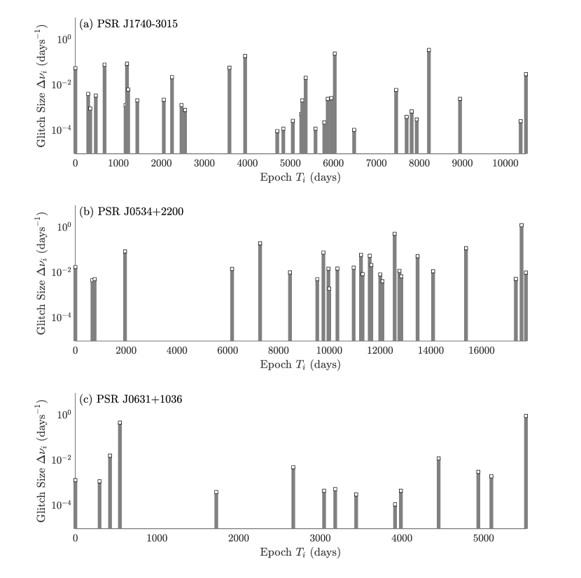
Figure 1: Time series of the observed glitch sizes $\Delta\nu_{i}$ (vertical axis; in ${\rm d}^{-1}$) and epochs $T_{i}$ (horizontal axis; in ${\rm d}$ since the first glitch) for PSR J1740$-$3015 (top panel), PSR J0534$+$2200 (middle panel), and PSR J0631$+$1036 (bottom panel). These data are used to estimate the parameters of the state-dependent Poisson model in §4 and predict future glitch epochs in §5.

4.1 Corner plots

Figures 2, 3, and 4 summarize the results of the MCMC estimation exercise pictorially for PSR J1740$-$3015, PSR J0534$+$2200, and PSR J0631$+$1036 respectively. Numerical values for the MCMC and PS maximum likelihood estimates of $\lambda_{0}$, $\tilde{t}_{0}$, $\tilde{X}_{0}$, $\tilde{X}(T_{1}^{+})$, $\delta$, and $\beta$ are quoted in Table 1 for the three objects. We start with $\gamma=2\pi$ for numerical convenience and extend to a range of $\gamma$ values in §4.3. Figures 2–4 are traditional corner plots. Every panel featuring colored contours corresponds to the likelihood marginalized over all but two parameters (e.g. $\lambda_{0}$ and $\beta$ in the bottom-left corner); yellow (blue) contours correspond to $\approx 0.9$ (0.09) times the maximum. Every panel featuring a single, black curve corresponds to the likelihood marginalized over all parameters but one (e.g. $\lambda_{0}$ in the top-left corner). In Table 1, the PS maximum likelihood estimates are quoted without error intervals, because we do not have the computational resources at our disposal to run a systematic suite of PS searches with different initializations for a seven-dimensional problem. However, the MCMC maximum likelihood estimates come with an error interval automatically attached (one-sigma half-width of the likelihood function).

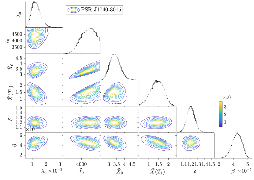
Figure 2: Corner plot of the likelihood for PSR J1740$-$3015 marginalized over all ${}^{6}C_{2}=15$ combinations of the parameters $\theta=\{\lambda_{0},\tilde{t}_{0},\tilde{X}_{0},\tilde{X}(T_{1}^{+}),\delta,\beta\}$. Ten evenly spaced contours are drawn between the maximum and minimum likelihoods in the MCMC sample, color-coded according to the color bar. Units: $\lambda_{0}$ in ${\rm d}^{-1}$, $\tilde{t}_{0}$ in d, $\tilde{X}_{0}$ and $\tilde{X}(T_{1}^{+})$ in ${\rm rad\,d^{-1}}$.

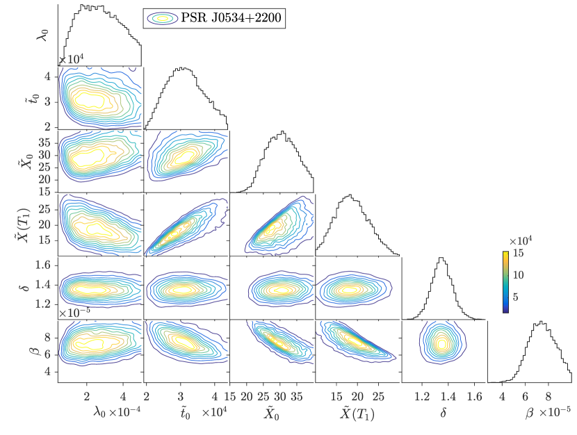
Figure 3: As for Figure 2 but for PSR J0534$+$2200.

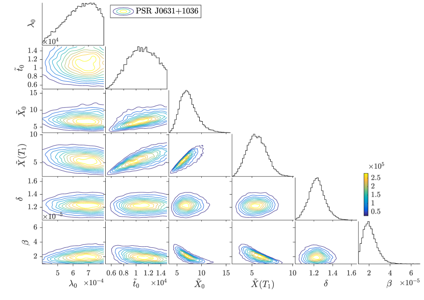
Figure 4: As for Figure 2 but for PSR J0631$+$1036.

PSR J	Method	$\lambda_{0}$	$\tilde{t}_{0}$	$\tilde{X}_{0}$	$\tilde{X}(T_{1}^{+})$	$\delta$	$\beta$
1740$-$3015	MCMC	$1.29\times 10^{-3}$	$4.35\times 10^{3}$	3.42	1.41	1.20	$4.5\times 10^{-5}$
		$\pm 3.3\times 10^{-4}$	$\pm 3.8\times 10^{2}$	$\pm 0.34$	$\pm 0.34$	$\pm 0.06$	$\pm 7\times 10^{-6}$
	PS	$1.04\times 10^{-3}$	$3.78\times 10^{3}$	2.89	1.34	1.21	$5.5\times 10^{-5}$
0534$+$2200	MCMC	$2.72\times 10^{-4}$	$3.14\times 10^{4}$	30.5	18.7	1.35	$7.5\times 10^{-5}$
		$\pm 1.1\times 10^{-4}$	$\pm 5.3\times 10^{3}$	$\pm 4.5$	$\pm 3.9$	$\pm 0.08$	$\pm 1\times 10^{-5}$
	PS	$1.08\times 10^{-4}$	$2.90\times 10^{4}$	25.9	18.5	1.36	$8.5\times 10^{-5}$
0631$+$1036	MCMC	$6.40\times 10^{-4}$	$1.10\times 10^{4}$	7.59	5.74	1.23	$2.0\times 10^{-5}$
		$\pm 9.7\times 10^{-5}$	$\pm 2.2\times 10^{3}$	$\pm 1.8$	$\pm 1.2$	$\pm 0.09$	$\pm 6\times 10^{-6}$
	PS	$4.91\times 10^{-4}$	$1.04\times 10^{4}$	6.70	6.04	1.24	$2.3\times 10^{-5}$

Table 1: MCMC and PS maximum likelihood estimates of the six parameters of the state-dependent Poisson process in §2 with $\gamma=2\pi$. The first (second) row of each MCMC entry contains the mean (standard deviation) of the likelihood function. Units: $\lambda_{0}$ in ${\rm d}^{-1}$, $\tilde{t}_{0}$ in d, $\tilde{X}_{0}$ and $\tilde{X}(T_{1}^{+})$ in ${\rm rad\,d^{-1}}$.

Despite the lack of formal confidence intervals on the PS estimates, we conclude that the PS and MCMC results are consistent on the whole. The PS estimate lies within the two-sigma MCMC error bar for every entry in Table 1 and within the one-sigma MCMC error bar for every entry except $\lambda_{0}$ and $\tilde{X}_{0}$ in PSR J0534$+$2200, $\tilde{t}_{0}$, $\tilde{X}_{0}$, and $\beta$ in PSR J1740$-$3015, and $\lambda_{0}$ in PSR J0631$+$1036. All the one- and two-variable likelihoods are unimodal. A detailed sensitivity analysis is computationally expensive and lies outside the scope of this paper. Instead we discuss what the estimates teach us physically, and how reasonable they are from the physical perspective, in §4.2 and §4.3.

4.2 Rate variables: $\tilde{t}_{0}$ and $\lambda_{0}$

The characteristic time-scale $\tilde{t}_{0}$ is $\sim 10$ times the mean observed waiting time for all three objects in Table 1. This is reasonable; the waiting times are bounded above by $\tilde{t}_{0}$ in the model in §2.

The microscopic trigger rate $\lambda_{0}$ is inferred to equal $\approx 6\tilde{t}_{0}^{-1}$ for all three objects in Table 1. In other words, $\lambda_{0}$ is within a factor of $\approx 2$ of the mean observed glitch rate. Again this is reasonable, because $X(t)$ spends most of the time fluctuating around $X(t)\sim 0.5$, yielding $\lambda[X(t)]\sim\lambda_{0}$. Interestingly, the maximum likelihood estimates yield $\alpha=\lambda_{0}\tilde{t}_{0}\approx 6$, cf. $\alpha_{\rm c}(\beta)\sim 1$. In other words, the objects spin down under but close to the critical rate and exhibit power-law size and exponential waiting time PDFs as expected.

4.3 Size variables: $\tilde{X}_{0}$, $\gamma$, $\beta$, and $\delta$

The characteristic angular velocity scale, $\tilde{X}_{0}$, ranges between $5\,\mu{\rm Hz}$ and $56\,\mu{\rm Hz}$ for the three objects in Table 1. From the observational perspective, this is reasonable. The above numbers are $\approx 10$ times larger than the maximum glitch size observed, and glitch size is bounded above by $\tilde{X}_{0}$ in the model in §2. From the theoretical perspective, $\tilde{X}_{0}=X_{\rm c}$ is consistent with sensible values of the maximum critical angular velocity lag in the superfluid vortex avalanche picture (Link & Epstein, 1991; Warszawski & Melatos, 2011), viz.

$$X_{\rm c}\leq 6\times 10^{-2}\left(\frac{F_{\rm max}}{{\rm kev\,fm^{-1}}}\right)\left(\frac{\rho}{10^{13}\,{\rm g\,cm^{-3}}}\right)^{-1}\left(\frac{l}{10^{2}\,{\rm fm}}\right)^{-1}\,{\rm Hz}~{},$$ (14)

where $F_{\rm max}$ is the maximum pinning force per nuclear lattice site, $\rho$ is the superfluid mass density, and $l$ is the pinning site separation. An analogous expression for the critical crustal stress in the starquake picture can be deduced from the models proposed by Middleditch et al. (2006) and Akbal & Alpar (2018); see also §5 in Melatos et al. (2018). The observed lack of strong size-waiting-time correlations in Poisson-like glitchers implies that the true critical lag is small compared to the maximum critical lag in (14); the stress reservoir never empties completely.

The minimum fractional avalanche size, $\beta$, satisfies $\beta\lesssim 10^{-4}\ll 1$ for the three objects in Table 1. In a fitting exercise of this kind, $\beta$ is expected to reflect the dynamic range of the observed glitch sizes. The observed glitches span $\approx 4\,{\rm dex}$ in the three objects, consistent with the maximum likelihood estimates of $\beta$. If future observations reveal even smaller events, the $\beta$ estimate will decrease. Conversely, if the smallest glitches observed to date are set by the resolution of the timing experiment, then the estimated value of $\beta$ is higher than the true, underlying, physical value, e.g. Janssen & Stappers (2006) but cf. Espinoza et al. (2014) for PSR J0534$+$2200.

The power-law exponents of the avalanche size PDF and observed glitch size PDF are equal in the theory in §2. Hence the PS and MCMC estimates of $\delta$ agree closely; they both reflect the well-defined shape of the observed glitch size PDF. They are also in accord with previous estimates of this quantity (Melatos et al., 2008; Ashton et al., 2017; Howitt et al., 2018; Shaw et al., 2018).

It turns out that maximizing ${\cal L}$ over $\gamma$ as well as the six parameters in Table 1 is too unwieldy even with human supervision, given the computational resources at our disposal. We therefore repeat the maximization in Table 1 for $\gamma=10$, 20, and 30 to gain an idea of how the results depend on $\gamma$. Overall, the dependence is weak: (i) $\lambda_{0}$ and $\tilde{t}_{0}$ change by $\lesssim 50$ per cent in opposite senses across the range, limiting the variation in $\alpha=\lambda_{0}\tilde{t}_{0}$ to $\lesssim 10$ per cent; (ii) $\tilde{X}_{0}$ and $\tilde{X}(T_{1}^{+})$ increase in rough proportion to $\gamma$, consistent with the appearance of $\gamma$ in (8) through the product $\gamma\Delta\nu_{i}$; (iii) $\beta$ decreases in rough proportion to $\gamma$; and (iv) $\delta$ changes by $\lesssim 10$ per cent.

When more data accumulate in the future, it will be interesting to study $\gamma$ in greater detail. The ratio of the crust and superfluid moments of inertia, which sets $\gamma$, is the subject of considerable theoretical uncertainty (Link et al., 1999; Andersson et al., 2012; Chamel, 2013; Piekarewicz et al., 2014; Eya et al., 2017). If the glitch-related angular momentum reservoir resides in the core superfluid, one expects $I_{\rm s}/I_{\rm c}\sim 10^{2}$ and $\gamma\lesssim 10^{3}$. Alternatively, if the reservoir resides in the inner crust, and the rigid crust and core superfluid are coupled magnetically by interactions between superfluid vortices and superconductor flux tubes, then one expects $I_{\rm s}/I_{\rm c}\sim 10^{-2}$ and $\gamma\approx 1$. The exact value of $\gamma$ depends on subtle microphysics, e.g. the strength of entrainment (Chamel, 2013) and the degree to which the vortices and flux tubes are tangled (Drummond & Melatos, 2018). Larger data sets have the potential to shed light on these interesting issues.

4.4 Stress history

Figure 5 displays the maximum likelihood estimates of the stress histories of the three objects in Table 1. We point out some key features. First, the trigger rate $\lambda(X)$ (middle column) varies substantially in all three objects, e.g. by a factor of $\approx 11$ from trough to peak in PSR J1740$-$3015. This is a general and slightly counterintuitive feature of the model in §2: the rate is variable, even though the waiting time PDF is consistent with a constant-$\lambda$ exponential to a good approximation; see §8 and Figure 24 in Fulgenzi et al. (2017). Second, $X(t)$ (left column) zig-zags more violently in PSR J1740$-$3015 than in PSR J0534$+$2200 and PSR J0631$+$1036. This is consistent with the $\delta$ estimates in the following sense. The long-term average $\langle\Delta\nu_{i}\rangle$ is dominated by the largest — and rarest — events for $\eta[X(T_{i}^{-})-\gamma\Delta\nu_{i}|X(T_{i}^{-})]\propto(\Delta\nu_{i})^{-\delta}$ and $1<\delta<2$. Hence it is normal for $X(t)$ to increase steadily over a relatively long interval, its rise interrupted by minor avalanches, before a large event strikes and resets $X(t)$ nearly to zero. Large events occur most frequently in PSR J1740$-$3015, whose $\delta$ value is the smallest of the three. Third, the histogram of the stresses $X(T_{i}^{+})$ ($1\leq i\leq N$) immediately after each glitch (right column) peaks at $0.5\lesssim X(T_{i}^{+})\lesssim 1$, consistent with the prediction by Fulgenzi et al. (2017); see Figure 21 in the latter reference.

Figure 5: Evolution of the stress variable in PSR J1740$-$3015 (top row), PSR J0534$+$2200 (middle row), and PSR J0631$+$1036 (bottom row). Left column. Maximum likelihood stress history, $X(t)$, normalized by the critical stress. Middle column. Dimensionless instantaneous glitch rate, $\lambda[X(t)]/\lambda_{0}=[1-X(t)]^{-1}$, versus time, $t$ (in MJD). Right column. Histogram of the normalized post-glitch stress, $X(T_{i}^{+})$ ($1\leq i\leq N$).

In Figure 6, we present an ensemble of stress histories $X(t)$ (left column) generated by Monte Carlo iteration of (1)–(5). For each object in Table 1, equations (1)–(5) are evaluated with the maximum likelihood estimate of the parameter vector $\theta$. It is clear by eye that many of the Monte Carlo stress histories (grey curves) resemble qualitatively the one that fits the observational data best (maximum ${\cal L}$; black curve). The size and waiting time cumulative distribution functions (CDFs) in the middle and right columns are also consistent with the data. Figure 6 therefore serves as a useful cross-check, that the maximum likelihood fit is not a statistical outlier.

Figure 6: Stress history $X(t)$ (left column), waiting time PDF $p(T_{i+1}-T_{i})$ (middle column; log linear axes), and size PDF $p(\gamma\Delta\nu_{i})$ (right column; log log axes) from Monte Carlo simulations of the model in §2 with the maximum likelihood estimate of $\theta$. The black, solid curves and grey, dotted curves indicate best-fitting and alternative stress histories respectively. Top row: PSR J1740$-$3015. Middle row: PSR J0534$+$2200. Bottom row: PSR J0631$+$1036. Parameters: as in Table 1; $10^{6}$ realizations per object.

The log likelihood (8) does not adjust for the measurement uncertainties in $T_{i}$ and $\Delta\nu_{i}$, because the formal errors quoted in the discovery papers are small (typically $\lesssim 5$ per cent in both variables), and the systematic errors are hard to quantify (Janssen & Stappers, 2006; Melatos et al., 2008; Espinoza et al., 2011; Yu & Liu, 2017). Generalizing ${\cal L}$ to include measurement uncertainties is a topic for future work. One interesting question is whether or not larger glitches, whose fractional measurement uncertainties are typically lower, are more informative about the maximum likelihood stress history than smaller glitches. In the analysis presented in this paper, the answer is no: all observed glitches above the minimum size set by $\beta$ in (5) are treated on an equal footing. In a fuller analysis including measurement uncertainties, the answer may be yes. Irrespective of measurement uncertainties, however, the constraint $\gamma\Delta\nu_{i}\leq X(T_{i}^{-})$ leading to (12) implies that larger glitches probe intervals, when $X(t)$ is closer to $X_{\rm c}$, and may influence the maximum likelihood estimate of $\tilde{X}_{0}$ more than smaller glitches. One can also ask: are larger glitches predicted more reliably than smaller glitches by the maximum likelihood model? Again the answer seems to be no. When we generate multiple Monte Carlo stress histories using the maximum likelihood estimate of $\theta$, as in Figure 6, the simulation is no better at predicting larger glitches at the observed epochs than smaller glitches, because the sizes are distributed as a power law and depend weakly on $X(T_{i}^{-})$ much of the time. Likewise, as the dispersion in waiting times for a Poisson process equals the mean, there is no reason to expect the Monte Carlo epochs in Figure 6 to coincide closely with the observed epochs on an individual basis. We merely expect the state-dependent Poisson model to predict epochs better than a homogeneous Poisson model on average, as discussed further in §5.

5 Epoch prediction

Even though the trigger rate $\lambda(X)$ varies $\gtrsim 10$-fold over the time intervals that PSR J1740$-$3015, PSR J0534$+$2200, and PSR J0631$+$1036 have been observed, the waiting time PDFs in all three objects are approximately exponential, as one would obtain for a homogeneous (i.e. constant-$\lambda$) Poisson process. It is therefore important to ask: is the predictive power of the state-dependent Poisson process in §2 any greater than a homogeneous Poisson process with the same average rate? The answer should be yes, because the model in §2 incorporates the extra information contained in the glitch sizes via the statistical correlation between $T_{i}-T_{i-1}$ and $X(T_{i}^{-})$ in (2). We quantify the relative performance below.

5.1 Validation against $T_{2},\dots,T_{N}$

We start by analysing the statistics of the errors in the epoch predictions of the state-dependent and homogeneous Poisson models when back-tested post factum against the historical epochs $T_{2},\dots,T_{N}$. Figure 7 displays histograms of the unsigned absolute error (i.e. absolute value of the predicted minus the true epoch) for all $T_{i}$ with $2\leq i\leq N$ for the three objects in Table 1. The associated means and standard deviations are summarized in Table 2. We find, as expected, that the state-dependent Poisson process is a better predictor than the homogeneous Poisson process. Importantly, though, the advantage is modest for the small samples available at present and it can be vitiated by an abnormally large, recent glitch. The mean error produced by the state-dependent Poisson model is $77$, $98$, and $73$ per cent of that produced by the homogeneous Poisson model for PSR J1740$-$3015, PSR J0534$+$2200 (minus the latest two glitches), and PSR J0631$+$1036 respectively. However, if the large, penultimate glitch in PSR J0534$+$2200 and its successor are included, the mean error of the state-dependent Poisson model rises to $108$ per cent of the homogeneous Poisson model (second line of Table 2). It drops back to $98$ per cent, if the first four glitches in PSR J0534$+$2200 are excluded (fourth line of Table 2), from the time before daily monitoring of the object commenced, when some small events may have been missed. For all three objects, the difference between the mean errors of the two models is smaller than their standard deviations. The dispersion in waiting times for any sort of Poisson process is typically comparable to the mean, due to the exponential form of (2), so wide error bars are the rule. In summary, therefore, the state-dependent Poisson model does not enjoy an unqualified advantage in epoch prediction over the homogeneous Poisson model for samples with $N\leq 35$ like those in Figure 7.

Figure 7: Histograms of the unsigned absolute error in the predicted epoch, i.e. the predicted minus the true epoch (measured in days), for $T_{2},\dots,T_{N}$ in (a) PSR J1740$-$3015, (b) PSR J0534$+$2200 and (c) PSR J0631$+$1036 for the state-dependent (red border) and homogeneous (blue border) Poisson models. The red and blue histograms overlap in some bins. Color-coded dots and horizontal error bars indicate the mean and standard deviation respectively for both models; see also Table 2.

PSR J	Mean (SDP)	Std dev (SDP)	Mean (HP)	Std dev (HP)
1740$-$3015	183.4	205.9	237.2	220.1
0534$+$2200	592.8	682.4	551.2	654.6
0534$+$2200	563.5	607.1	573.7	666.5
0534$+$2200	381.6	309.0	389.5	303.7
0631$+$1036	167.2	112.7	229.6	215.3

Table 2: Means and standard deviations of the error histograms in Figure 7 for the state-dependent (SDP) and homogeneous (HP) Poisson models. All entries are measured in days.

The histograms in Figure 7 unavoidably blend together two factors: the goodness-of-fit of each model, and the improved ability of each model to make predictions, as the sample of events grows. For example, both models are expected to perform better at predicting $T_{100}$ than $T_{2}$, statistically speaking. This is illustrated in Figure 8, where the error is graphed versus event number for both Poisson models. PSR J1740$-$3015 is chosen for this figure because it has the largest number of glitches. The early events ($2\leq i\leq 14$) are not plotted, because the scatter is large and uninformative; both models struggle to predict epochs with insufficient information. For intermediate events ($15\leq i\lesssim 25$), the scatter is lower, and the errors produced by the two models are comparable. For later events ($25\lesssim i\leq 35$), the red and blue curves separate, and the state-dependent Poisson model performs slightly better. Again, though, the performance difference is small compared to the dispersion. There is no strong, sustained decrease in the error produced by the state-dependent Poisson model over the range $15\leq i\leq 35$, confirming that the existing event sample is small.

Figure 8: Unsigned absolute error in the predicted epoch (in days) versus event number $i$ ($15\leq i\leq 35$) for the state-dependent (solid red curve) and homogeneous (dashed blue curve) Poisson models for PSR J1740$-$3015. The shading (with the same color coding) denotes the one-sigma error bars for the two models. Events with $2\leq i\leq 14$ are not plotted, because the scatter is large and uninformative.

Ideally, the histograms in Figure 7 would be redrawn for (say) $T_{50}$ for a large number of objects, but this is impossible with existing data. Instead we perform a numerical Monte Carlo simulation along the same lines and present the results in Appendix B. It is found that the predictive advantage of the state-dependent Poisson model asserts itself increasingly for $N\gtrsim 50$, as the information embedded in the glitch sizes increasingly constrains $X(t)$ and hence $\lambda[X(t)]$. That is, the mean error from the state-dependent Poisson model is lower than from the homogeneous Poisson model, and the standard deviation scales $\propto N^{-1/2}$ as expected. The Monte Carlo trend in the standard deviation contrasts somewhat with the real data from PSR J1740$-$3015, analysed in Figure 8, where there is no obvious shrinkage in the shaded red band at $i\approx 35$ relative to $i\lesssim 25$. It is unclear whether or not this is a statistical accident; more data are needed to resolve the issue. We emphasize that the results in Appendix B apply in an astrophysical setting only to the extent that the glitch microphysics conforms to the meta-model of a state-dependent Poisson process.

5.2 The next glitch: $T_{N+1}$

We conclude this section by presenting falsifiable epoch predictions for the next glitches to occur in the three objects in Table 1. Epochs and one-sigma error bars are tabulated in Table 3 for the state-dependent Poisson model in §2. Assuming the model is a faithful description of Poisson-like glitch activity, the central tendencies of the predicted epochs are $T_{36}=57784$ (MJD) for PSR J1740$-$3015, $T_{29}=60713$ (MJD) for PSR J0534$+$2200, and $T_{16}=57406$ (MJD) for PSR J0631$+$1036. Analogous, falsifiable predictions can be made for these or other Poisson-like glitchers in the future following the recipe in this paper, as more events are discovered.

PSR J	Mean $T_{N+1}$	Std dev
1740$-$3015	57784	256.8
0534$+$2200	60713	1935
0631$+$1036	57406	1444

Table 3: Mean predicted epoch (MJD) and one-sigma uncertainty (in days) of the next glitch in each of the objects in Table 1, based on the state-dependent Poisson model.

6 Conclusion

A state-dependent Poisson process of the form (1)–(5) generates power-law size and exponential waiting time PDFs in the slow-spin-down regime $\alpha\gtrsim\alpha_{\rm c}\sim 1$. It is a plausible meta-model for glitch activity in pulsars that do not glitch quasiperiodically, whether the glitch microphysics involves starquakes, superfluid vortex avalanches, or some other stress growth-release mechanism. In this paper we compute maximum likelihood estimates for the seven parameters governing the dynamics described by (1)–(5) for the three Poisson-like pulsars with the most events: PSR J1740$-$3015, PSR J0534$+$2200, and PSR J0631$+$1036. We find that MCMC and PS maximization algorithms produce similar estimates, with $3\leq\alpha\leq 9$, trigger rate $1\times 10^{-4}\leq\lambda_{0}/(1\,{\rm d^{-1}})\leq 1\times 10^{-3}$, stress threshold $3\leq X_{\rm c}/(1\,{\rm rad\,d^{-1}})\leq 31$, minimum fractional avalanche size $2\times 10^{-5}\leq\beta\leq 9\times 10^{-5}$, and a weak dependence on the moment-of-inertia ratio ($\alpha\approx{\rm constant}$, $X_{c}\propto\gamma$, $\beta\propto\gamma^{-1}$ approximately) in the fiducial range $6\leq\gamma\leq 30$. The maximum likelihood estimates are tabulated in Table 1 and cross-checked for consistency against Monte Carlo simulations. Parameter estimation of this sort is a promising tool for probing the glitch microphysics in the future, when more data become available. For example, improved estimates of $\lambda_{0}$ and $\gamma$ may shed light on the glitch trigger mechanism and site of the angular momentum reservoir respectively.

The trigger rate $\lambda[X(t)]=\lambda_{0}[1-X(t)]^{-1}$ varies more than 10-fold in the inferred maximum likelihood stress histories of the above three objects, so it is pertinent to ask whether or not a state-dependent Poisson model delivers more accurate epoch predictions than a homogeneous Poisson model. Back-testing against historical glitches indicates that the answer is a qualified yes for the above three objects, but the improvement is small both fractionally (7–27 per cent) and compared to the dispersion and can be reversed by an abnormally large, recent glitch (e.g. in PSR J0534$+$2200). Monte Carlo simulations indicate that a sample with $N\gtrsim 50$ is needed, in order to test reliably whether or not the state-dependent Poisson model outperforms. Falsifiable predictions are made that the epoch of the next glitch in the three tested objects is $T_{36}=57784$ (MJD) for PSR J1740$-$3015, $T_{29}=60713$ (MJD) for PSR J0534$+$2200, and $T_{16}=57406$ (MJD) for PSR J0631$+$1036, with associated one-sigma error intervals. The predicted epochs stand alongside falsifiable predictions concerning auto- and cross-correlations between sizes and waiting times, which can be tested independently (Melatos et al., 2018; Carlin & Melatos, 2019a). For example, Melatos et al. (2018) identified PSR J0205$+$6449 as one of five pulsars likely to exhibit a strong cross-correlation between sizes and forward waiting times with the advent of more data [see Table 2 in Melatos et al. (2018)]. The prediction found support recently in a reanalysis based on twice as many events (Fuentes et al., 2019) but it could have been falsified just as easily. We emphasize again that the state-dependent Poisson model does not apply to quasiperiodic glitchers in the form introduced by Fulgenzi et al. (2017).

In order to make the most of the opportunity for falsification, more glitches need to be discovered. As well as monitoring more objects with higher duty cycle, e.g. with phased arrays (Kramer & Stappers, 2010; Caleb et al., 2016), it is worth exploring how to reduce the minimum resolvable glitch size, in case there is a populous tail of smaller glitches waiting to be discovered in some objects [although arguably not in PSR J0534$+$2200; see Espinoza et al. (2014)]. Algorithms that harness the power of distributed volunteer computing (Clark et al., 2017) or take a Bayesian approach to inferring glitch parameters (Shannon et al., 2016) are set to play a role in delivering these and other improvements.

Appendix A Supervised, iterative, numerical recipe for maximizing ${\cal L}$

In this paper, we maximize the likelihood ${\cal L}$ defined by (8) with respect to the parameter set $\theta$ by executing the following, iterative, step-by-step recipe, which combines two species of automated numerical maximization algorithms with human supervision based on screening the intermediate results.

(i) We set bounds on the parameters using a combination of the data, order-of-magnitude estimates, and internal consistency constraints satisfied by (1)–(5). The bounds are specified in §3.1.

(ii) Working by hand, we run Monte Carlo simulations of (1)–(5) at a small number of random points in the parameter space. In each time series $X(t)$ generated thus, we check whether or not certain key glitch features (e.g. average size, maximum size, average waiting time, latest epoch) match the data approximately. When one bound on a variable is finite and the other is infinite, we start searching near the finite bound and gradually step further away. This part of the recipe is not systematic and relies on human discretion.

(iii) From the small set of ad hoc experiments in step (ii), we record the parameter vector $\theta^{\prime}$ with the highest ${\cal L}$. This rudimentary estimate serves as a safety check on the algorithmic searches to follow. If the algorithms return a completely different parameter vector with even higher ${\cal L}$, it counts as good news. On the other hand, if the algorithms settle on a lower ${\cal L}$, there are grounds for concern. We also generate synthetic, Monte Carlo data for $\theta^{\prime}$, feed the data to the algorithms, and check if the algorithms return $\theta^{\prime}$.

(iv) Starting and staying within the bounds established in step (i) and explored in steps (ii) and (iii), we run two automatic maximization algorithms, particle swarm (PS) and Markov chain Monte Carlo (MCMC). Details of the algorithms and their use are given in §3.2. As an example, for the three objects studied in this paper, the supervised experiments in steps (ii) and (iii) yield the following bounds for the automated maximisation algorithms: $\lambda_{0}\in[0,1]$ (in units of ${\rm d}^{-1}$), $\tilde{t}_{0}\in[\max_{i}(T_{i+1}-T_{i}),20\max_{i}(T_{i+1}-T_{i})]$, $\gamma^{-1}\tilde{X}_{0}\in[\max_{i}(\Delta\nu_{i}),20\max_{i}(\Delta\nu_{i})]$, $\delta\in[0,2]$, $\beta\in[0,1]$, and $\gamma\in[2\pi,30]$. These bounds are used for all the PS searches. The more expensive MCMC searches are done over a smaller region, centred around the PS point estimates, in order to compute the marginalized likelihoods.

(v) We check the results from step (iv) against those from step (iii). Optionally one can also run a brute force grid scan and a genetic algorithm (for example) in the vicinity of the maxima returned in step (iv) where necessary and appropriate. If any of these safety checks uncover a higher local maximum, we return to step (iv) and run PS and MCMC again with a refined starting point.

Appendix B Epoch prediction with homogeneous and state-dependent Poisson processes

In this appendix, we compare the predictive accuracy of (i) a homogeneous Poisson process with a constant rate equal to the reciprocal of the arithmetic mean of the observed waiting times, and (ii) a state-dependent Poisson process of the form specified in §2, whose variable rate is generated by the stress history $X(t)$ corresponding to the maximum likelihood estimates of the parameters $\tilde{X}_{0}$, $\tilde{t}_{0}$, $\alpha$ (or equivalently $\lambda_{0}$), $X(T_{1}^{+})$, $\gamma$, $\beta$, and $\delta$. The motivation for the comparative study is the results from §4 and §5, which suggest that (ii) is a marginally better epoch predictor than (i). The latter conclusion is tentative: it is reached in only three pulsars and for relatively small samples ($N\leq 35$) and reverses if certain events are excluded, e.g. the unusually large, penultimate glitch in PSR J0534$+$2200 (see Table 2). Below we employ Monte Carlo simulations to study the matter further and obtain improved statistics. Needless to say, the simulations cannot address the question of whether (i) or (ii) is a better epoch predictor for a real pulsar; this will be resolved in the future, as more astronomical data become available. The simulations simplify verify the expected result that, if a state-dependent Poisson process is hypothetically at work in a pulsar, then (ii) is a better epoch predictor than (i), because (ii) is calibrated against the observed sizes and waiting times and allows $\lambda[X(t)]$ to vary, while (i) is calibrated against the waiting times only and holds $\lambda[X(t)]$ constant artificially.

Figures 9 and 10 confirm that the parameters of the state-dependent Poisson model are estimated with increasing accuracy, as $N$ increases. Equations (1)–(5) are used to generate $96\times 2$ realizations of $X(t)$ with $N=20$ and $N=100$ for $\theta$ as specified in the caption of Figure 9. The PS algorithm is applied to the synthetic data to produce maximum likelihood point estimates of $\lambda_{0}$, $\tilde{t}_{0}$, $\tilde{X}_{0}$, $\tilde{X}(T_{1}^{+})$, $\beta$, and $\delta$. (We fix $\gamma=2\pi$ as in §4.1–§4.3 to keep the computation tractable.) The estimates are plotted pairwise to assist with visualization in Figure 9, with blue and red dots corresponding to $N=20$ and $N=100$ respectively. One finds that the red dots are clustered more tightly around the true values (grey horizontal and vertical lines) than the blue dots, as expected. Figure 10 makes the same point by presenting histograms for the normalized distance between the true and estimated parameters, as defined by the six-dimensional Euclidean norm. One finds that the $N=100$ histogram is narrower than the $N=20$ histogram; its mean and standard deviation are $\lesssim 4$ times smaller.

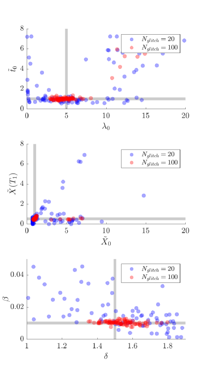
Figure 9: Dispersion of parameter estimates for PS searches of synthetic data generated by (1)–(5) containing 20 glitches (shaded red circles; 96 realizations) and 100 glitches (shaded blue circles; 96 realizations), visualized via three two-dimensional cross-sections of the parameter space: $\tilde{t}_{0}$ versus $\lambda_{0}$ (top panel), $\tilde{X}(T_{1})$ versus $\tilde{X}_{0}$ (middle panel), and $\beta$ versus $\delta$ (bottom panel), with $\gamma=2\pi$ fixed. The grey shaded lines denote the true parameter values: $\lambda_{0}=5$, $\tilde{t}_{0}=1$, $\tilde{X}_{0}=1$, $\tilde{X}(T_{1}^{+})=0.5$, $\delta=1.5$, $\beta=0.01$.

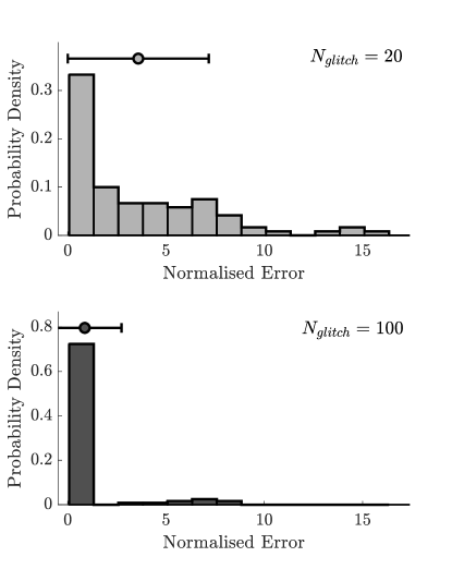
Figure 10: Normalized error between the true parameter values $\theta$ and PS estimates $\hat{\theta}$ for the Monte Carlo simulations in Figure 9 for $N=20$ (top histogram; 96 realizations) and $N=100$ (bottom histogram; 96 realizations). The normalized error is defined as the six-dimensional Euclidean norm, $[\sum_{j=1}^{6}(\theta_{j}-\hat{\theta}_{j})^{2}/\theta_{j}^{2}]^{1/2}$, with $\gamma=2\pi$ fixed. The mean and standard deviation are 3.59 and 3.59 for $N=20$ and $0.87$ and $1.87$ for $N=100$ respectively.

Figure 11 confirms that epoch predictions based on a state-dependent Poisson model are more accurate than epoch predictions based on a homogeneous Poisson model, if a state-dependent Poisson process governs the underlying dynamics. Although by itself this is not surprising, the purpose of Figure 11 is to quantify roughly how many events are needed, before the advantage asserts itself clearly. Histograms are presented of the unsigned absolute error in the predicted epochs $T_{2},\dots,T_{N}$ for $N=20$ and $N=100$, computed for $96\times 2$ realizations of $X(t)$ for a state-dependent Poisson process with the same parameters as in Figure 9. The state-dependent and homogeneous Poisson models are equally accurate for $N=20$, but the former outperforms the latter for $N=100$, where its mean error is 11 per cent smaller; see Table 4. The advantage is modest, for the reasons expressed in §5.1. The Monte Carlo simulations can be extended to study how the error in predicting $T_{N+1}$ scales with $N$, when warranted by additional data. Again we emphasize that the Monte Carlo results say nothing about whether glitch activity in real pulsars obeys a state-dependent Poisson process.

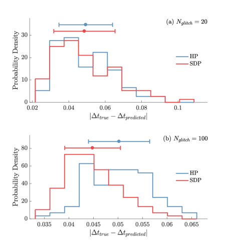
Figure 11: Histogram of the unsigned absolute error in the (dimensionless) predicted epoch, i.e. the predicted minus the true epoch inferred from the state-dependent (red border) and homogeneous (blue border) Poisson models, for the Monte Carlo simulations in Figure 9. (a) $T_{2},\dots,T_{20}$. (b) $T_{2},\dots,T_{100}$. The red and blue histograms overlap in some bins. Color-coded dots and horizontal error bars indicate the mean and standard deviation respectively for both models; see also Table 4.

$N$	Mean (SDP)	Std dev (SDP)	Mean (HP)	Std dev (HP)
20	0.0486	0.0422	0.0493	0.0414
100	0.0448	0.0420	0.0502	0.0461

Table 4: Means and standard deviations of the (dimensionless) epoch prediction error histograms in Figure 11 versus the number of glitches $N$ for the state-dependent (SDP) and homogeneous (HP) Poisson models.

References

- Akbal & Alpar (2018) Akbal O., Alpar M. A., 2018, MNRAS, 473, 621
- Akbal et al. (2017) Akbal O., Alpar M. A., Buchner S., Pines D., 2017, MNRAS, 469, 4183
- Alpar et al. (1984) Alpar M. A., Pines D., Anderson P. W., Shaham J., 1984, ApJ, 276, 325
- Andersson et al. (2012) Andersson N., Glampedakis K., Ho W. C. G., Espinoza C. M., 2012, Physical Review Letters, 109, 241103
- Ashton et al. (2017) Ashton G., Prix R., Jones D. I., 2017, Phys. Rev. D, 96, 063004
- Brooks et al. (2011) Brooks S., Gelman A., Jones G., Meng X.-L., 2011, Handbook of Markov Chain Monte Carlo
- Caleb et al. (2016) Caleb M., Flynn C., Bailes M., Barr E. D., Bateman T., Bhandari S., Campbell-Wilson D., Green A. J., Hunstead R. W., Jameson A., Jankowski F., Keane E. F., Ravi V., van Straten W., Krishnan V. V., 2016, MNRAS, 458, 718
- Carlin & Melatos (2019a) Carlin J. B., Melatos A., 2019a, MNRAS, 488, 4890
- Carlin & Melatos (2019b) Carlin J. B., Melatos A., 2019b, MNRAS, 483, 4742
- Carlin et al. (2019) Carlin J. B., Melatos A., Vukcevic D., 2019, MNRAS, 482, 3736
- Chamel (2013) Chamel N., 2013, Physical Review Letters, 110, 011101
- Chugunov & Horowitz (2010) Chugunov A. I., Horowitz C. J., 2010, MNRAS, 407, L54
- Clark et al. (2017) Clark C. J., Wu J., Pletsch H. J., Guillemot L., Allen B., Aulbert C., Beer C., Bock O., Cuéllar A., Eggenstein H. B., Fehrmann H., Kramer M., Machenschalk B., Nieder L., 2017, ApJ, 834, 106
- Clerc (2010) Clerc M., 2010, Particle Sawrm Optimization
- Daly & Porporato (2007) Daly E., Porporato A., 2007, Phys. Rev. E, 75, 011119
- Del Moral & Penev (2017) Del Moral P., Penev S., 2017, Stochastic Processes: From Applications to Theory
- Drummond & Melatos (2018) Drummond L. V., Melatos A., 2018, MNRAS, 475, 910
- Edwards et al. (2006) Edwards R. T., Hobbs G. B., Manchester R. N., 2006, MNRAS, 372, 1549
- Espinoza et al. (2014) Espinoza C. M., Antonopoulou D., Stappers B. W., Watts A., Lyne A. G., 2014, MNRAS, 440, 2755
- Espinoza et al. (2011) Espinoza C. M., Lyne A. G., Stappers B. W., Kramer M., 2011, MNRAS, 414, 1679
- Eya et al. (2017) Eya I. O., Urama J. O., Chukwude A. E., 2017, ApJ, 840, 56
- Ferdman et al. (2018) Ferdman R. D., Archibald R. F., Gourgouliatos K. N., Kaspi V. M., 2018, ApJ, 852, 123
- Fuentes et al. (2019) Fuentes J. R., Espinoza C. M., Reisenegger A., 2019, arXiv e-prints, p. arXiv:1907.09887
- Fulgenzi et al. (2017) Fulgenzi W., Melatos A., Hughes B. D., 2017, MNRAS, 470, 4307
- Haskell & Melatos (2015) Haskell B., Melatos A., 2015, International Journal of Modern Physics D, 24, 1530008
- Hobbs et al. (2006) Hobbs G., Edwards R., Manchester R., 2006, Chinese Journal of Astronomy and Astrophysics Supplement, 6, 189
- Howitt et al. (2018) Howitt G., Melatos A., Delaigle A., 2018, ApJ, 867, 60
- Janssen & Stappers (2006) Janssen G. H., Stappers B. W., 2006, A&A, 457, 611
- Jensen (1998) Jensen H. J., 1998, Self-Organized Criticality. Cambridge: University Press
- Kingman (1993) Kingman J. F., 1993, Poisson Processes
- Kramer & Stappers (2010) Kramer M., Stappers B., 2010, in ISKAF2010 Science Meeting LOFAR, LEAP and beyond: Using next generation telescopes for pulsar astrophysics
- Link et al. (1999) Link B., Epstein R. I., Lattimer J. M., 1999, Physical Review Letters, 83, 3362
- Link & Epstein (1991) Link B. K., Epstein R. I., 1991, ApJ, 373, 592
- Lyne & Graham-Smith (2012) Lyne A., Graham-Smith F., 2012, Pulsar Astronomy
- Melatos et al. (2015) Melatos A., Douglass J. A., Simula T. P., 2015, ApJ, 807, 132
- Melatos et al. (2018) Melatos A., Howitt G., Fulgenzi W., 2018, ApJ, 863, 196
- Melatos et al. (2008) Melatos A., Peralta C., Wyithe J. S. B., 2008, ApJ, 672, 1103
- Mezura-Montes & Coello Coello (2011) Mezura-Montes E., Coello Coello C., 2011, Swarm and Evolutionary Computation, 1, 173
- Middleditch et al. (2006) Middleditch J., Marshall F. E., Wang Q. D., Gotthelf E. V., Zhang W., 2006, ApJ, 652, 1531
- Onuchukwu & Chukwude (2016) Onuchukwu C. C., Chukwude A. E., 2016, Ap&SS, 361, 300
- Piekarewicz et al. (2014) Piekarewicz J., Fattoyev F. J., Horowitz C. J., 2014, Phys. Rev. C, 90, 015803
- Pitkin & Romano (2018) Pitkin M., Romano J., , 2018, mattpitkin/matlabmultinest: v0.1
- Shabanova (2009) Shabanova T. V., 2009, ApJ, 700, 1009
- Shannon et al. (2016) Shannon R. M., Lentati L. T., Kerr M., Johnston S., Hobbs G., Manchester R. N., 2016, MNRAS, 459, 3104
- Shaw et al. (2018) Shaw B., Lyne A. G., Stappers B. W., Weltevrede P., Bassa C. G., Lien A. Y., Mickaliger M. B., Breton R. P., Jordan C. A., Keith M. J., Krimm H. A., 2018, MNRAS, 478, 3832
- Veitch & Vecchio (2010) Veitch J., Vecchio A., 2010, Phys. Rev. D, 81, 062003
- Warszawski & Melatos (2011) Warszawski L., Melatos A., 2011, MNRAS, 415, 1611
- Warszawski & Melatos (2013) Warszawski L., Melatos A., 2013, MNRAS, 428, 1911
- Wheatland (2008) Wheatland M. S., 2008, ApJ, 679, 1621
- Wong et al. (2001) Wong T., Backer D. C., Lyne A. G., 2001, ApJ, 548, 447
- Yu & Liu (2017) Yu M., Liu Q.-J., 2017, MNRAS, 468, 3031
- Yu et al. (2013) Yu M., Manchester R. N., Hobbs G., Johnston S., Kaspi V. M., Keith M., Lyne A. G., Qiao G. J., Ravi V., Sarkissian J. M., Shannon R., Xu R. X., 2013, MNRAS, 429, 688
- Yuan et al. (2010) Yuan J. P., Wang N., Manchester R. N., Liu Z. Y., 2010, MNRAS, 404, 289