Covariant calculation of a two-loop test of
nonrelativistic QCD factorization

Abstract

We test the nonrelativistic QCD factorization conjecture for inclusive quarkonium production at two loops by carrying out a covariant calculation of the nonrelativistic quantum chromodynamics (NRQCD) long-distance matrix element (LDME) for a heavy-quark pair in an $S$-wave, color-octet state to fragment into a heavy-quark pair in a color-singlet state of arbitrary orbital angular momentum. The NRQCD factorization conjecture for the universality of the LDME requires that infrared divergences that it contains be independent of the direction of the Wilson line that appears in its definition. We find this to be the case in our calculation. The results of our calculation differ in some respects from those of a previous calculation that was carried out by Nayak, Qiu, and Sterman using light-cone methods. We have identified the sources of some of these differences. The results of both calculations are consistent with the NRQCD factorization conjecture. However, the general principle that underlies this confirmation of NRQCD factorization at two-loop order has yet to be revealed.

I Introduction

The nonrelativistic quantum chromodynamics (NRQCD) factorization conjecture for inclusive quarkonium production in hard-scattering QCD processes Bodwin:1994jh postulates that the production rates for those processes at large momentum transfer can be written as a sum of products of short-distance coefficients (SDCs) and NRQCD long-distance matrix elements (LDMEs). The SDCs are process dependent, but they contain no infrared (IR) divergences, and can be calculated in perturbation theory. The LDMEs contain all of the IR sensitivity of the process. They are generally nonperturbative in nature, but they are conjectured to be universal (process independent)—a property that gives NRQCD factorization much of its predictive power.

The NRQCD factorization conjecture has enjoyed considerable phenomenological success. (See, for example, Refs. Brambilla:2004wf ; Brambilla:2010cs ; Lansberg:2019adr .) However, there are also processes for which theory and experiment are in considerable tension. (See, for example, Refs. Brambilla:2010cs ; Lansberg:2019adr .)

Although the NRQCD factorization conjecture has been in existence for many years, there is still no demonstration that it is correct to all orders in perturbation theory or that it fails in perturbation theory. Important progress toward an all-orders proof of NRQCD factorization was presented in Ref. Nayak:2005rt . There, an all-orders argument was given, for the leading and first subleading powers of $m_{H}/p_{T}$, that quarkonium production rates can be written as a sum of SDCs convolved with fragmentation functions for one or two partons to fragment into a quarkonium. Here, $m_{H}$ and $p_{T}$ are the mass and transverse momentum, respectively, of the quarkonium.

A proof of NRQCD factorization would require the further factorization of the fragmentation functions into sums of products of SDCs with NRQCD LDMEs. (In the remainder of this paper, when we refer to SDCs, we mean the SDCs that relate the LDMEs to fragmentation functions.) One difficulty in carrying out this factorization is that the fragmentation functions at the scale of the heavy-quark mass $m_{Q}$ contain processes in which gluons are radiated with energies of order $m_{Q}$ in the quarkonium center-of-momentum (c.m.) frame. Such gluons cannot be absorbed into the NRQCD LDMEs, which contain radiation only at the small scale $m_{Q}v$, where $v$ is the typical velocity of the heavy quark $Q$ or antiquark $\bar{Q}$ in the quarkonium c.m. frame. On the other hand, soft gluons with arbitrarily small momenta can connect the order-$m_{Q}$ gluons to the $Q$ or $\bar{Q}$, and these soft gluons must be absorbed into the NRQCD LDME if NRQCD factorization is to hold. A resolution of this dilemma was suggested in Ref. Nayak:2005rt . It is based on modifying the original definition of an LDME to include a Wilson line, which acts as a proxy for an order-$m_{Q}$ gluon, in that its interactions with additional soft gluons are identical to those of the order-$m_{Q}$ gluon. This so-called “gauge completion” of the LDMEs is also required in order to make the LDMEs manifestly gauge invariant Nayak:2005rt . (In this paper, we will always refer to the gauge-completion Wilson lines as “Wilson lines” in order to distinguish them from soft approximations to the heavy-quark lines, which we refer to as “eikonal lines.”)

There are no apparent obstacles to establishing that all of the soft singularities in the fragmentation functions can be absorbed into the gauge-completed NRQCD LDMEs, given that the effective field theory NRQCD is a valid approximation to QCD in the soft limit and that the gauge-completed LDMEs account for the soft interactions with the order-$m_{Q}$ gluons. The central problem in proving NRQCD factorization is then to demonstrate that the soft divergences in the LDMEs are independent of the direction(s) of the gauge-completion Wilson line(s). Without such a demonstration, the LDMEs would depend on the directions of the order-$m_{Q}$ gluons, and so universality of the LDMEs would be lost, even for a single type of quarkonium production process.

Let us contrast this situation with that in exclusive quarkonium production. A proof of NRQCD factorization for exclusive quarkonium production at leading power in the inverse of the hard-scattering momentum transfer is given in Refs. Bodwin:2008nf ; Bodwin:2009cb . That proof focuses on a demonstration that soft-gluon contributions that do not decouple from the quarkonium can be absorbed completely into the quarkonium jet. The proof does not address the further factorization of the quarkonium jet into NRQCD LDMEs. In the proof, it was assumed, on general grounds, that this factorization would be valid, since NRQCD is the effective field theory that describes the relevant low-energy degrees of freedom. As we have mentioned, the issue of the dependence of the LDMEs on the Wilson-line direction arises in inclusive quarkonium production because of the emission of gluons with energies of order $m_{Q}$ in the quarkonium c.m. frame. Such real-gluon emissions do not occur in exclusive quarkonium production, and so no Wilson line is needed to account for their couplings to soft gluons. Furthermore, the relevant vacuum-to-quarkonium matrix elements have color-singlet quantum numbers and do not require a gauge-completion Wilson line. Therefore, the issue of dependence on the direction of a Wilson line never arises in this case.

A proof of factorization for inclusive quarkonium decays is also qualitatively different from a proof for inclusive quarkonium production. It is thought that NRQCD factorization for inclusive quarkonium decays can be established along the lines of the argument that is given in Ref. Bodwin:1994jh , although no complete proof has been published. The essential element of this argument is that contributions of final-state soft or collinear gluons that are radiated from final-state hard partons cancel in an inclusive process because of the Kinoshita-Lee-Nauenberg theorem. Because soft gluons decouple from the hard-scattering subdiagram, no Wilson line is needed in this case to account for soft-gluon exchanges between hard gluons (with energies of order $m_{Q}$) and the heavy quark or antiquark. Furthermore, the decay LDMEs do not require a gauge-completion Wilson line. Again, the issue of dependence on the direction of a Wilson line never arises in this case.

Returning to the case of inclusive quarkonium production, we note that perturbative tests at one and two loops of the proposition that the soft divergences in the LDMEs are independent of the direction of the gauge-completion Wilson line have been provided by Nayak, Qiu, and Sterman Nayak:2005rw ; Nayak:2005rt ; Nayak:2006fm . In Refs. Nayak:2005rw ; Nayak:2005rt , one- and two-loop contributions to the LDMEs were given at the leading nontrivial order in $v$ (order $v^{2}$), with the details of the calculations being given in Ref. Nayak:2005rt . In Ref. Nayak:2006fm , the one- and two-loop contributions were given to all orders in $v$, although explicit expressions were given only for the non-Abelian diagrams, which are the most complicated to evaluate. The calculations in these papers confirmed that the soft divergences in the LDMEs are independent of the Wilson-line direction through two loops. In the remainder of this paper, we refer collectively to Refs. Nayak:2005rt ; Nayak:2006fm as “NQS”.

The calculations in Refs. Nayak:2005rw ; Nayak:2005rt ; Nayak:2006fm make use of light-cone methods, in which one first uses contour integration to carry out the integration over the component of a loop momentum that lies in the minus light-cone direction. The calculations also make use of hard ultraviolet (UV) cutoffs for the phase-space integrations for real gluons. Hence, the calculations are not manifestly Lorentz invariant at intermediate stages, although the final results are. The calculations are quite complicated, especially for the non-Abelian diagrams, and the independence of the soft divergences from the Wilson-line direction emerges only after many complicated intermediate expressions are summed. Therefore, it seems worthwhile to check these calculations using manifestly covariant methods. One could hope that such covariant calculations might give insights into the independence of the soft divergences from the Wilson-line direction.

In this paper, we present such a manifestly covariant calculation of the soft divergences in an LDME at two-loop order. The calculation relies on a new UV regulator for the phase-space integrations that avoids the use of a hard cutoff. As we will see, our covariant calculation is actually considerably more complicated than the calculations in NQS. This is probably because the light-cone methods in NQS allow one to cancel contributions of real-real diagrams against contributions of real-virtual diagrams and to cancel certain real-virtual contributions by symmetry, without having to calculate them completely. In contrast, in our calculations, we compute all of the IR contributions of the real-real diagrams and real-virtual diagrams explicitly and implement cancellations only at the end. Consequently, we must deal with soft poles in dimensional regularization in $D=4-2\epsilon$ dimensions of order $1/\epsilon^{4}$, $1/\epsilon^{3}$, $1/\epsilon^{2}$, and $1/\epsilon$ in order to arrive at a final result of order $1/\epsilon$. Although we can eliminate the $1/\epsilon^{4}$ contribution trivially at the start by making a Ward-identity rearrangement of the numerator structure, we still must work out the cancellation of the $1/\epsilon^{3}$ and $1/\epsilon^{2}$ poles, while the NQS calculation contains only $1/\epsilon^{2}$ imaginary poles, which cancel in the absolute square of the amplitude, and $1/\epsilon$ real poles.

In NQS, it was found that IR poles in the LDME are independent of the Wilson-line direction, and we also find that to be the case. Our result for the non-Abelian diagrams agrees with that in NQS, aside from an overall sign. Our result for the Abelian diagrams differs from that in NQS in two respects. First, we find new contributions that have the form of a one-loop contribution to an SDC times the one-loop IR-divergent contribution to the LDME. For these contributions, the IR pole in the LDME is independent of the direction of the Wilson line. We conclude that some of these contributions are absent in NQS because a mismatch between virtual-gluon and real-gluon contributions in the UV region was neglected. We also find a new contribution that has the form of a two-loop IR-divergent contribution to the LDME. Again, the IR pole in the LDME is independent of the direction of the Wilson line. This new contribution can be reconciled with the result in NQS if we reinterpret a UV contribution in NQS as an IR contribution.

The remainder of this paper is organized as follows. In Sec. II we describe the LDME and its Feynman rules, the classes of diagrams that we calculate, and the kinematics. Section III contains a description of the covariant phase-space regulator that we use and also contains convenient formulas for the phase-space integration in dimensional regularization. The main body of our work is in Sec. IV, in which we give a description of the calculations for the various diagrams. Because the extraction of analytic expressions for the coefficients of the IR poles is not straightforward, we present our calculation in considerable detail, so that an interested reader would be able to reproduce our results. We have relegated the technical details of the calculation to appendices. Our results are summarized in Sec. V, and we compare them with the results in NQS in Sec.VI. Finally, we give our conclusions in Sec. VII.

II Preliminaries

The gauge-completed LDME is given by Nayak:2006fm

$$\langle{\mathcal{O}}^{H}_{n}(0)\rangle=\langle 0|\chi^{\dagger}(0){\mathcal{K}}_{n,e}\psi(0)\Phi_{\ell}^{(A)}{}^{\dagger}(0){}_{eb}\left(a^{\dagger}_{H}a_{H}\right)\Phi_{\ell}^{(A)}(0)_{ba}\psi^{\dagger}(0){\mathcal{K}}^{\prime}_{n,a}\chi(0)|0\rangle,$$ (1)

where $\psi^{\dagger}$ and $\chi$ are two-component Pauli fields that create a heavy quark and a heavy antiquark, respectively, $\mathcal{K}_{n,e}$ and $\mathcal{K^{\prime}}_{n,a}$ are local combinations of spin and color matrices and polynomials in covariant derivatives, and $a_{H}^{\dagger}$ is the operator that creates the quarkonium $H$. The operators $\Phi_{\ell}^{(A)}(0){}$ are Wilson lines, which are defined by

$$\Phi_{\ell}^{(A)}(0){} = \mathcal{P}\text{exp}\left[-ig_{s}\int_{0}^{\infty}d\lambda\,\ell\cdot A^{(A)}(\ell\lambda)\right],$$ (2)

where $\mathcal{P}$ stands for path ordering, $g_{s}=\sqrt{4\pi\alpha_{s}}$ is the QCD coupling constant, $A^{(A)\mu}=A^{\mu}_{a}t_{a}$ is the gauge field in the adjoint representation, $(t_{a})_{bc}=-if_{abc}$, and $\ell^{\mu}$ is the momentum of the Wilson line.

Following NQS, we consider the LDME for a $Q\bar{Q}$ pair in an $S$-wave, color-octet state to evolve into a $Q\bar{Q}$ pair in a color-singlet state of arbitrary orbital angular momentum. That is, we consider the matrix elements Nayak:2006fm

$${\cal M}^{(8\to I)}(P_{1},P_{2},\ell) = \sum_{X}\langle 0|\chi^{\dagger}(0)T^{(q)}_{e}\psi(0)\Phi_{\ell}^{(A)}{}^{\dagger}(0){}_{eb}|[Q(P_{1})\bar{Q}(P_{2})]^{(I)}X\rangle$$ (3)

$$\times\langle X[Q(P_{1})\bar{Q}(P_{2})]^{(I)}|\Phi_{\ell}^{(A)}(0)_{ba}\psi^{\dagger}(0)T^{(q)}_{a}\chi(0)|0\rangle,$$

where the superscript $I=1,\,8$ denotes the color of the $Q\bar{Q}$ pair, the $T_{i}^{(q)}$ are the generators of color SU$(3)$ in the fundamental representation, and $P_{1}$ and $P_{2}$ are momenta of $Q$ and $\bar{Q}$, respectively. We do not explicitly consider the spin state of the $Q\bar{Q}$ pair, as the soft approximation for the $Q$ and $\bar{Q}$ lines is independent of the spin.

In computing the matrix elements in Eq. (3), we encounter factors that arise from UV-divergent loop integrals. Since these factors contain no IR sensitivity, they can be interpreted as contributions to the SDCs that relate the LDMEs to fragmentation functions. As we have mentioned, the directions of the Wilson lines correspond to the directions of emitted gluons that have energies of order $m_{Q}$ in the quarkonium c.m. frame. Therefore, the directions of the Wilson lines are process dependent, and the SDCs, which are process dependent, can depend on the directions of the Wilson lines. Dependence of the SDCs on the Wilson-line directions is entirely consistent with NRQCD factorization, provided that the IR poles, which are absorbed into the LDMEs, are independent of the Wilson-line directions.

The only one-loop contribution to the matrix element in Eq. (3) that has a nonvanishing color factor is shown in Fig. 1. The superscripts $P_{j}P_{k}$ specify the gluon connections to the $Q$ or $\bar{Q}$ lines on either side of the cut.

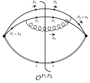
Figure 1: The one-loop diagram $\mathcal{O}^{P_{1}P_{2}}$

Now let us consider the two-loop diagrams that contribute to the matrix element in Eq. (3). Since we wish to test for a dependence on the direction of the LDME Wilson line, we need to consider only those diagrams in which at least one gluon attaches to the Wilson line. Furthermore, it is clear that a diagram has a nonzero color factor only if one or more gluons crosses the final-state cut. The specific classes of diagrams that we compute are illustrated in Figs. 3–7. We use the notation ${\mathcal{X}}_{i}^{P_{j}P_{k}}$ for the contributions of these diagrams. Here, ${\mathcal{X}}_{i}$ denotes the class of the diagram. For each class, the subscript $i$ labels the position of the final-state cut, and the superscripts $P_{j}P_{k}$ specify the gluon connections to the $Q$ and $\bar{Q}$ lines, as we will describe below. The classes are defined as follows.

• $\mathcal{A}_{i}^{P_{j}P_{k}}$ (Fig. 3) designates normal ladder diagrams. $P_{j}$ indicates the leftmost gluon connection to the heavy-quark lines; $P_{k}$ indicates the rightmost gluon connection to the heavy-quark lines.

• $\mathcal{B}_{i}^{P_{j}P_{k}}$ (Fig. 3) designates crossed ladder diagrams. $P_{j}$ indicates the leftmost gluon connection to the heavy-quark lines; $P_{k}$ indicates the rightmost gluon connection to the heavy-quark lines.

• $\mathcal{C}_{i}^{P_{j}P_{k}}$ (Fig. 6) designates Abelian diagrams with two connections of gluons to the same heavy-quark line to the left of the cut, in which the gluon that connects to the Wilson line connects to the heavy-quark line to the left of the other gluon. $P_{j}$ indicates the two leftmost connections of gluons to the heavy-quark lines; $P_{k}$ indicates the rightmost connection of a gluon to the heavy-quark lines.

• $\mathcal{D}_{i}^{P_{j}P_{k}}$ (Fig. 6) designates Abelian diagrams with two connections of gluons to different heavy-quark lines to the left of the cut. $P_{j}$ indicates the leftmost connection to the heavy-quark lines of the gluon that does not attach to the Wilson line; $P_{k}$ indicates the rightmost connection to the heavy-quark lines of the gluon that does not attach to the Wilson line.

• $\mathcal{E}_{i}^{P_{j}P_{k}}$ (Fig. 6) designates Abelian diagrams with two connections of gluons to the same heavy-quark line to the left of the cut, in which the gluon that connects to the Wilson line connects to the heavy-quark line to the right of the other gluon. $P_{j}$ indicates the two leftmost connections of gluons to the heavy-quark lines; $P_{k}$ indicates the rightmost connection of a gluon to the heavy-quark lines.

• $\mathcal{F}_{i}^{P_{j}P_{k}}$ (Fig. 7) designates the non-Abelian diagrams. $P_{j}$ indicates the leftmost connection of a gluon to the heavy-quark lines; $P_{k}$ indicates the rightmost connection of a gluon to the heavy-quark lines.

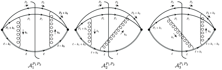
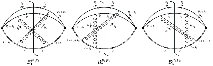
Figure 2: Ladder diagrams $\mathcal{A}_{i}^{P_{1}P_{2}}$

Figure 3: Crossed ladder diagrams $\mathcal{B}_{i}^{P_{1}P_{2}}$

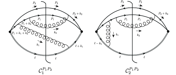
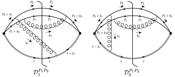
Figure 4: Diagrams $\mathcal{C}_{i}^{P_{1}P_{2}}$

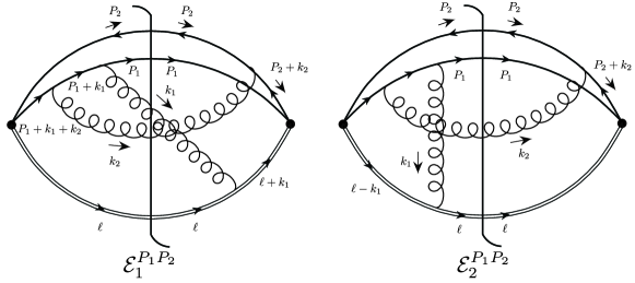
Figure 5: Diagrams $\mathcal{D}_{i}^{P_{1}P_{2}}$

Figure 6: Diagrams $\mathcal{E}_{i}^{P_{1}P_{2}}$

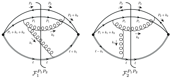
Figure 7: Non-Abelian diagrams $\mathcal{F}_{i}^{P_{1}P_{2}}$

The classes of diagrams are constructed such that one can obtain all of the contributions that we calculate by summing over the indices $i$, $j$, and $k$ and including Hermitian-conjugate diagrams, except for the classes $\mathcal{A}$ and $\mathcal{B}$, for which the sums over the indices $i$, $j$, and $k$ already include the Hermitian-conjugate contributions. We note that the assignments of our loop momenta $k_{1}$ and $k_{2}$ for the diagrams $\mathcal{C}_{i}$, $\mathcal{D}_{i}$, $\mathcal{E}_{i}$, and $\mathcal{F}_{i}$ are different from those of NQS.

We define the total momentum of the $Q\bar{Q}$ pair to be $2p$ and the relative momentum to $Q\bar{Q}$ rest frame to be $q$, and so

$$P_{1}=p+q,\quad P_{2}=p-q.$$ (4)

In the rest frame of the $Q\bar{Q}$ pair, $p$ and $q$ are given by

$$p=(E_{Q},\bm{0}),\quad q=(0,\bm{q}),$$ (5)

where $E_{Q}=\sqrt{m_{Q}^{2}+\bm{q}^{2}}$. The relative velocity of the $Q$ and $\bar{Q}$ is

$$\bm{v}=\frac{2\bm{q}}{E_{Q}}.$$ (6)

In comparing with the light-cone calculation in NQS, we need to make use of light-cone momentum coordinates for a $D$-dimensional vector $V=(V^{0},V^{1},\cdots,V^{D-1})$, which we take to be

$$V^{+} = \frac{1}{\sqrt{2}}\left(V^{0}+V^{D-1}\right),$$

$$V^{-} = \frac{1}{\sqrt{2}}\left(V^{0}-V^{D-1}\right),$$

$$\bm{V}_{\perp} = (V^{1},V^{2},\cdots,V^{D-2}).$$ (7)

Then, a scalar product of two vectors $V$ and $W$ is given by

$$V\cdot W = V^{0}W^{0}-V^{D-1}W^{D-1}-\bm{V}_{\perp}\cdot\bm{W}_{\perp}$$ (8)

$$= V^{+}W^{-}+V^{-}W^{+}-\bm{V}_{\perp}\cdot\bm{W}_{\perp}.$$

We note that, in NQS, the momentum of the Wilson line is specified to be along the minus light-cone direction:

$$\ell=(\ell^{+},\ell^{-},\bm{\ell}_{\perp})=(0,1,\bm{0}_{\perp}).$$ (9)

However, our covariant calculation does not make use of this assignment.

We define the following Lorentz-invariant quantities, which appear throughout our calculations:

$$P_{1}^{2}=P_{2}^{2},\quad\ell^{2}=0,\quad a=\frac{P_{1}\cdot P_{2}}{P_{1}^{2}},\quad c=\frac{P_{1}\cdot\ell}{P_{1}^{2}},\quad d=\frac{P_{2}\cdot\ell}{P_{1}^{2}}.$$ (10)

Since we are interested in analyzing the soft singularities, we take soft approximations for the interactions of the gluons with the $Q$ and $\bar{Q}$ lines. As we have mentioned, we refer to the $Q$ and $\bar{Q}$ lines in the soft approximation as “eikonal lines,” and we refer to the gauge-completion Wilson lines as “Wilson lines,” in order to distinguish them from each other. The Feynman rules for the eikonal lines and Wilson lines are given in Refs. Nayak:2005rt ; Nayak:2006fm . They are summarized below.

• The interaction between a gluon and a $Q$ or $\bar{Q}$ line to the left of the final-state cut is shown in Fig. 8. The propagator for a $Q$ or $\bar{Q}$ line to the left of the cut is given by

  $$\frac{i}{P_{i}\cdot k+i\varepsilon},$$ (11)

  and the vertex is given by

  $$\quad-ig_{s}\mu^{\epsilon}(T_{a})_{bc}P_{i}^{\alpha},$$ (12)

  where $\alpha$ is the Lorentz index of the vertex, $a$ is the color index of the vertex, $b$ and $c$ are the color indices of the $Q$, $\mu^{\epsilon}$ is introduced to account for the dimensionality of the coupling constant in $D=4-2\epsilon$ dimensions, and the diagrammatic momentum of the $\bar{Q}$ line is opposite to the physical momentum. The rules for propagators and vertices to the right of the final-state cut are obtained by taking the Hermitian conjugates of the rules that are shown. Note that the product of a propagator and a vertex is invariant with respect to a change of the scale of $P_{i}$.

  

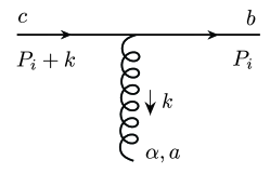
  Figure 8: Gluon interaction with a $Q$ or $\bar{Q}$ line.

• The interaction of a gluon with a Wilson line is illustrated in Fig. 9. On the left side of the final-state cut, the Wilson-line propagator is given by

  $$\frac{-i}{\ell\cdot k+i\varepsilon},$$ (13)

  and the vertex is given by

  $$-g_{s}\mu^{\epsilon}\ell^{\alpha}f_{abc},$$ (14)

  where $a,\,b,\,c$ are color indices and the $f_{abc}$ are the structure constants of SU$(3)$. The rules for propagators and vertices to the right of the final-state cut are obtained by taking the Hermitian conjugates of the rules that are shown. As in the eikonal-line case, the product of a Wilson-line propagator and vertex is invariant with respect to a change of the scale of line momentum $\ell$.

  

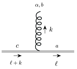
  Figure 9: Gluon interaction with a Wilson line.

The Feynman rules for the non-eikonal and non-Wilson-line parts of the diagram are the usual ones. We follow the conventions in Sterman:1994ce , which are consistent with the conventions that we have chosen for the eikonal and Wilson lines. We work in the Feynman gauge throughout.

We find that our expressions for the diagrams $\mathcal{C}_{i}$, $\mathcal{D}_{i}$, $\mathcal{E}_{i}$, and $\mathcal{F}_{i}$, which contain one gluon connection to the Wilson line, differ by an overall sign from the expressions for the corresponding diagrams in NQS.

III Phase Space

In this section we discuss the covariant phase-space regulators that we employ and also present convenient formulas for carrying out the phase-space integrations in dimensional regularization.

III.1 Phase-space regulators

Because the eikonal and Wilson propagator denominators are linear in the loop momenta and the eikonal and Wilson vertices are independent of the loop momenta, the unregulated expressions for the LDME are invariant under a simultaneous rescaling of both loop momenta. This scale invariance would lead to a vanishing of the unregulated loop integrations in dimensional regularization. That is, UV poles from the loop integrations would cancel IR poles from the loop integrations. However, our goal is to isolate and calculate the IR poles. We accomplish this by imposing an additional UV regulator, which breaks the scale invariance of the integrals and guarantees that our results contain only IR poles.

In the fragmentation function in which the LDME is embedded, there are restrictions on the final-state phase space that follow from Dirac $\delta$ functions that express conservation of the light-cone energy:

$$\begin{cases}\delta\left[\ell\cdot(k-P_{1}-P_{2}-k_{2})\right],\quad\hbox{when the gluon with momentum $k_{2}$ is real},\\ \delta\left[\ell\cdot(k-P_{1}-P_{2}-k_{1}-k_{2})\right],\quad\hbox{when the gluons with momenta $k_{1}$ and $k_{2}$ are real}.\end{cases}$$ (15)

Here $k$ is the momentum of the parton (gluon) that fragments into the $Q\bar{Q}$ pair. In the fragmentation function at a scale of order $m_{Q}$, the light-cone energy that is available to the final-state gluons, $\ell\cdot k^{\prime}=\ell\cdot(k-P_{1}-P_{2}$), is also of order $m_{Q}$.

Motivated by this constraint on the fragmentation-function phase space, we impose a UV cutoff on the phase space of the LDME. In NQS, there is also a UV cutoff on the phase space of the LDME. It is imposed as a hard cutoff on $\ell\cdot k^{\prime}$ (and on the remaining components of $k^{\prime}$). We find it calculationally more convenient to provide a cutoff of order $m_{Q}$ on $\ell\cdot k^{\prime}$ by applying a weight function to the available light-cone energy $\ell\cdot k^{\prime}$:

$$w(\ell\cdot k)\equiv\frac{\Lambda^{2}}{2(\ell\cdot k)+\Lambda^{2}},$$ (16)

where $\Lambda$ is a cutoff parameter of order $m_{Q}$. Then, integrating over the constraints in Eq. (15), we obtain

$$\int_{0}^{\infty}d(\ell\cdot k^{\prime})w(\ell\cdot k^{\prime})\,\delta\left[\ell\cdot(k^{\prime}-k_{2})\right]=\frac{\Lambda^{2}}{2\ell\cdot k_{2}+\Lambda^{2}},$$ (17a)

when the gluon with momentum $$k_{2}$$ is real, and

$$\int_{0}^{\infty}d(\ell\cdot k^{\prime})w(\ell\cdot k^{\prime})\,\delta\left[\ell\cdot(k^{\prime}-k_{1}-k_{2})\right]=\frac{\Lambda^{2}}{2\ell\cdot(k_{1}+k_{2})+\Lambda^{2}},$$ (17b)

when the gluons with momenta $k_{1}$ and $k_{2}$ are real. We call the factors on the right side of Eq. (17) our standard phase-space regulators. For some parts of the calculation, as we will explain later, we will find it necessary to impose temporarily additional UV regulators in order to ascertain the IR or UV nature of poles in $\epsilon$.

III.2 Phase-space integration

In computing the phase-space integration for the final-state gluons, it is convenient to extend the range of integration to infinity, relying on UV regulators to remove UV poles. Then, we obtain the following phase-space integration formulas:

$$\int_{k}\textrm{PS}\frac{1}{(2p\cdot k+M^{2}\pm i\varepsilon)^{s}} = \frac{1}{(4\pi)^{\frac{D}{2}}}\frac{\Gamma(\frac{D}{2}-1)\Gamma(s-D+2)}{\Gamma(s)\left(p^{0}+|\bm{p}|\pm i\varepsilon\right)^{\frac{D}{2}-1}\left(p^{0}-|\bm{p}|\pm i\varepsilon\right)^{\frac{D}{2}-1}(M^{2}\pm i\varepsilon)^{s-D+2}},$$

$$\int_{k}\textrm{PS}\frac{k^{\alpha}}{(2p\cdot k+M^{2}\pm i\varepsilon)^{s}} = \frac{p^{\alpha}}{(4\pi)^{\frac{D}{2}}}\frac{\Gamma(\frac{D}{2})\Gamma(s-D+1)}{\Gamma(s)\left(p^{0}+|\bm{p}|\pm i\varepsilon\right)^{\frac{D}{2}}\left(p^{0}-|\bm{p}|\pm i\varepsilon\right)^{\frac{D}{2}}\left(M^{2}\pm i\varepsilon\right)^{s-D+1}},$$

where $p^{0}$ is the temporal component of $p$, $\bm{p}$ is the vector of spatial components of $p$, and we define the measure of the phase-space integration as

$$\int_{k}\textrm{PS}\equiv\int\frac{d^{D}k}{(2\pi)^{D}}2\pi\delta(k^{2})\theta(k^{0}).$$ (19)

In all of the calculations in this paper, we have arranged the parameter integrations so that $p^{0}+|\bm{p}|>0$ and $p^{0}-|\bm{p}|>0$. In this case the first two denominator factors in Eq. (18) can be written as $(p^{2})^{\frac{D}{2}-1}$, and the first two denominator factors in Eq. (18) can be written as $(p^{2})^{\frac{D}{2}}$. The derivation of the formulas in Eq. (18) is given in Appendix B.

IV Analyses of the diagrams

In this section, we outline our calculations for the various classes of diagrams.

IV.1 Method of calculation

Our general method of calculation is as follows.

For the Abelian diagrams, we carry out the $k_{1}$ integration first, holding $k_{2}$ fixed. We control UV divergences by imposing our standard phase-space regulators and, in some cases, temporarily impose additional UV regulators in order to determine the IR or UV nature of the poles in $\epsilon$. We first combine the denominators by using Feynman parameters that run from 0 to 1 to combine denominators that have a common term involving $k_{1}$ and by using Feynman parameters that run from 0 to $\infty$ to combine the remaining denominators. We then carry out the integration over $k_{1}$, using standard formulas of dimensional regularization if $k_{1}$ is virtual and using Eq. (18) if $k_{1}$ is real. We identify the singular regions of the parameter integrals and isolate these as integrations over a single parameter, either by rescaling the parameters that run from 0 to $\infty$ or, in a few cases, by using sector decomposition. We then expand the integrals around the singularities by making use of formulas such as

$$\frac{1}{x^{1+a\epsilon}}=-\frac{1}{a\epsilon}\delta(x)+\left[\frac{1}{x}\right]_{+}-a\epsilon\left[\frac{\log x}{x}\right]_{+}+O(\epsilon^{2}),$$ (20)

which applies when the domain of integration is $0\leq x\leq 1$. Here, the plus distribution $[g(x)]_{+}$ is defined by

$$\int_{0}^{1}dx\,f(x)[g(x)]_{+}\equiv\int_{0}^{1}dx[f(x)-f(0)]g(x),$$ (21)

for a regular function $f(x)$ in $x\in[0,1]$. However, we avoid expanding factors involving $k_{2}$ in powers of $\epsilon$, as the complete $\epsilon$ dependence of these factors is needed to find the coefficient of the soft pole from the $k_{2}$ integration.

We find for the Abelian diagrams that the $k_{1}$ integrations for the sum over a class plus Hermitian conjugate are IR finite when $k_{2}$ is fixed. In some cases, there are UV poles from the $k_{1}$ integration. The IR finiteness of the $k_{1}$ integration when $k_{2}$ is fixed is expected on general principles because the sum over cuts in a class is sufficient to effect a unitarity cancellation of singularities that occur when $k_{1}$ is soft relative to $k_{2}$ or $k_{1}$ is collinear to $\ell$.

Some of the contributions from the $k_{1}$ integration remain finite as $k_{2}$ goes to zero, and these can be considered to be SDCs that multiply possible one-loop IR poles from the $k_{2}$ integration. In the cases of diagrams $\mathcal{C}$ and $\mathcal{E}$, there are contributions that become singular as $k_{2}$ goes to zero, and these yield two-loop IR-divergent contributions to the LDME.

Once we have evaluated the $k_{1}$ integration, we can carry out the $k_{2}$ integration straightforwardly by combining denominators with Feynman parameters and using Eq. (18) to carry out the phase-space integration. The remaining parameter integrals are easily reduced, by using expansions of the type in Eq. (20), to elementary integrals.

In the case of the non-Abelian diagrams, the $k_{1}$ integration for the sum over the class plus Hermitian conjugate is no longer IR finite when $k_{2}$ is held fixed. In this case, as we will explain, the unitarity cancellation requires that one carry out the $k_{2}$ integration, as well as the $k_{1}$ integration. Therefore, for the non-Abelian diagrams, we combine denominators involving both $k_{1}$ and $k_{2}$ using Feynman parameters that range from 0 to 1 or from 0 to $\infty$, as outlined above. We then carry out the $k_{1}$ and $k_{2}$ integrations, isolate the IR singularities in single-parameter integrals by using rescaling or sector decomposition, and evaluate the IR poles by using Eq. (20).

In most cases, we have checked the results from direct integration of the parameter integrals by using the Mellin-Barnes representation to decompose a denominator so as to obtain parameter integrations that can be carried out in terms of beta functions. We then evaluate the Mellin-Barnes integrations by isolating poles in $\epsilon$, using the methods of Tausk Tausk:1999vh or Smirnov Smirnov:2004ym , and computing the remaining finite integrals as a sum over residues in the complex plane of Mellin-Barnes integration variable.

IV.2 The one-loop IR contribution to the LDME

The color factor of the $\mathcal{O}$ diagram (Fig. 1) is given by

$$C_{\mathcal{O}^{P_{j}P_{k}}}=\frac{\textrm{Tr}(T_{a}T_{b})}{\sqrt{N_{c}}}\frac{\textrm{Tr}(T_{a}T_{b})}{\sqrt{N_{c}}}=\frac{\delta_{aa}}{4N_{c}}=\frac{N_{c}^{2}-1}{4N_{c}}.$$ (22)

The expression for the diagram $\mathcal{O}$, with our standard phase-space regulators in Eq. (17), is given by

$$\mathcal{O}^{P_{1}P_{2}} = \frac{4g_{s}^{2}a}{(P_{1}^{2})^{-1}}\times\mu^{2\epsilon}\int_{k_{2}}\textrm{PS}\frac{\Lambda^{2}}{\left(2P_{1}\cdot k_{2}\right)\left(2P_{2}\cdot k_{2}\right)\left(2\ell\cdot k_{2}+\Lambda^{2}\right)}.$$ (23)

Combining the denominators by using Feynman parameters and carrying out the $k_{2}$ phase-space integration by using Eq. (18), we find that

$$\mu^{2\epsilon}\int_{k_{2}}\textrm{PS}\,\frac{\Lambda^{2}}{(2P_{1}\cdot k_{2})(2P_{2}\cdot k_{2})\left(2\ell\cdot k_{2}+\Lambda^{2}\right)}$$

$$= \mu^{2\epsilon}\Lambda^{2}\frac{\Gamma(3)}{\Gamma(1)}\int_{0}^{\infty}d\lambda_{2}\int_{0}^{\infty}d\lambda_{3}\int_{k_{2}}\textrm{PS}\,\frac{1}{\left[2k_{2}\cdot(\ell+\lambda_{2}P_{1}+\lambda_{3}P_{2})+\Lambda^{2}\right]^{3}}$$ (24)

$$= -\frac{\left(\frac{\tilde{\mu}^{2}P_{1}^{2}}{\Lambda^{4}}\right)^{\epsilon}}{(4\pi)^{2}P_{1}^{2}}\frac{e^{\epsilon\gamma_{{}_{\textrm{E}}}}\Gamma(1+2\epsilon)\Gamma(1-2\epsilon)\Gamma(1+\epsilon)}{2\epsilon_{\textrm{IR}}}\int_{0}^{\infty}d\xi\frac{1}{A^{1+\epsilon}B^{-2\epsilon}}$$

$$= -\frac{1}{(4\pi)^{2}P_{1}^{2}}\frac{1}{2\epsilon_{\textrm{IR}}}\frac{\log\left(a+\sqrt{a^{2}-1}\right)}{\sqrt{a^{2}-1}}+O(\epsilon^{0}),$$

where $\tilde{\mu}^{2}\equiv 4\pi\mu^{2}e^{-\gamma_{{}_{\textrm{E}}}}$, $\gamma_{{}_{\textrm{E}}}$ is the Euler-Mascheroni constant, and we have made the change of variables $\lambda_{3}\to\xi\lambda_{2}$, carried out $\lambda_{2}$ integration in terms of the beta function, introduced the definitions

$$A \equiv \xi^{2}+2a\xi+1,$$

$$B \equiv 1+\frac{d}{c}\xi,$$ (25)

and carried out the $\xi$ integration by using Eq. (A).

Then, taking into account the color factor in Eq. (22) and summing over the gluon attachments, we obtain

$$\mathcal{O} \equiv \sum_{j=1}^{2}\sum_{k=1}^{2}C_{\mathcal{O}^{P_{j}P_{k}}}\mathcal{O}^{P_{j}P_{k}}$$ (26)

$$= \left[\frac{\alpha_{s}}{4\pi}\frac{N_{c}^{2}-1}{4N_{c}}\frac{4}{\epsilon_{\textrm{IR}}}\left(1-\frac{a\log\left(a+\sqrt{a^{2}-1}\right)}{\sqrt{a^{2}-1}}\right)+O(\epsilon^{0})\right]_{\textrm{IR}}.$$

If we expand Eq. (26) to leading order in $\bm{q}^{2}$, then it agrees with the expression in Eq. (38) of Ref. Nayak:2005rt , aside from the color factor, which has been dropped in Ref. Nayak:2005rt .

IV.3 $\mathcal{A}_{i}$ diagrams

We do not need to evaluate the momentum integrations for $\mathcal{A}_{i}$ diagrams, as the color factors vanish:

$$C_{\mathcal{A}_{i}^{P_{j}P_{k}}} = \frac{\textrm{Tr}\left[T^{a}T^{b}\right]}{\sqrt{N_{c}}}\frac{\textrm{Tr}\left[T^{c}T^{d}\right]}{\sqrt{N_{c}}}f_{abe}f_{ced}=\frac{f_{aae}f_{cec}}{4N_{c}}=0.$$ (27)

IV.4 $\mathcal{B}_{i}$ diagrams

The color factors of the $\mathcal{B}_{i}$ diagrams are given by

$$C_{\mathcal{B}_{i}^{P_{j}P_{k}}} = \frac{\textrm{Tr}\left[T^{a}T^{b}\right]}{\sqrt{N_{c}}}\frac{\textrm{Tr}\left[T^{c}T^{d}\right]}{\sqrt{N_{c}}}f_{cbe}f_{dae}=\frac{f_{cae}f_{cae}}{4N_{c}}=\frac{N_{c}(N_{c}^{2}-1)}{4N_{c}}.$$ (28)

The Feynman amplitudes for the $\mathcal{B}_{i}^{P_{1}P_{2}}$ diagrams with our standard phase-space regulators are given by

$$\mathcal{B}_{1}^{P_{1}P_{2}} = \frac{16g_{s}^{4}\Lambda^{2}cd}{(P_{1}^{2})^{-2}}\mu^{4\epsilon}\int_{k_{2}}\textrm{PS}\,\frac{1}{(2P_{2}\cdot k_{2})(2\ell\cdot k_{2})}\int_{k_{1}}\textrm{PS}\,\frac{1}{(2P_{1}\cdot k_{1})(2\ell\cdot k_{1})\left[2\ell\cdot(k_{1}+k_{2})+\Lambda^{2}\right]},$$

$$\mathcal{B}_{2}^{P_{1}P_{2}} = \frac{16ig_{s}^{4}\Lambda^{2}cd}{(P_{1}^{2})^{-2}}\mu^{4\epsilon}\int_{k_{2}}\textrm{PS}\,\frac{1}{(2P_{2}\cdot k_{2})(2\ell\cdot k_{2}+\Lambda^{2})}$$

$$\times\int\frac{d^{D}k_{1}}{(2\pi)^{D}}\frac{1}{(2P_{1}\cdot k_{1}+i\varepsilon)(-2\ell\cdot k_{1}+i\varepsilon)(k_{1}^{2}+i\varepsilon)\left[2\ell\cdot(-k_{1}+k_{2})+i\varepsilon\right]},$$

$$\mathcal{B}_{3}^{P_{1}P_{2}} = -\frac{16ig_{s}^{4}\Lambda^{2}cd}{(P_{1}^{2})^{-2}}\mu^{4\epsilon}\int_{k_{1}}\textrm{PS}\,\frac{1}{\left(2P_{1}\cdot k_{1}\right)\left(2\ell\cdot k_{1}+\Lambda^{2}\right)}$$ (29)

$$\times\int\frac{d^{D}k_{2}}{(2\pi)^{D}}\,\frac{1}{\left(2P_{2}\cdot k_{2}-i\varepsilon\right)\left(-2\ell\cdot k_{2}-i\varepsilon\right)\left(k_{2}^{2}-i\varepsilon\right)\left[2\ell\cdot(k_{1}-k_{2})-i\varepsilon\right]},$$

where $c$ and $d$ are defined in Eq. (10) and we have suppressed unnecessary $i\varepsilon$’s in the denominators.

IV.4.1 IR finiteness of the $k_{1}$ or $k_{2}$ integration

We wish to establish that, for a certain combination of the $\mathcal{B}_{i}$, the integration over $k_{1}$ with $k_{2}$ fixed is IR finite, while for the remaining part of the $\mathcal{B}_{i}$ the integration over $k_{2}$ with $k_{1}$ fixed is IR finite. For this purpose, we temporarily impose additional regulators to control all of the UV divergences.

It can be seen by power counting that our standard UV regulators render the integrations over $\ell\cdot k_{1}$ and $\ell\cdot k_{2}$ UV finite. However, there are still potential UV divergences that could arise from the integrations over the other components of $k_{1}$ and $k_{2}$. In order to control these divergences, we introduce the following additional UV-regulator factor

$$\frac{\Lambda^{\prime\hskip 0.49005pt4}}{(2P_{1}\cdot k_{1}+\Lambda^{\prime\hskip 0.49005pt2})(2P_{2}\cdot k_{2}+\Lambda^{\prime\hskip 0.49005pt2})},$$ (30)

where the cutoff $\Lambda^{\prime}$ is of order $m_{Q}$. We denote the $\mathcal{B}_{i}$ into which we have inserted this UV-regulator factor by $\mathcal{B}_{i}\big{|}_{\textrm{Reg}}$.

The $\mathcal{B}_{i}$ contain rapidity (collinear) divergences that are associated with the vanishing of the denominators of Wilson-line propagators. We expect these divergences to cancel, because of unitarity, in the sum over cuts of the $\mathcal{B}_{i}$. We can separate the parts of $\mathcal{B}_{1}$ that contribute to the cancellations of the rapidity divergences in $\mathcal{B}_{2}$ and $\mathcal{B}_{3}$ by making use of the following partial-fraction identity in $\mathcal{B}_{1}^{P_{1}P_{2}}\big{|}_{\textrm{Reg}}$:

$$\frac{1}{(2\ell\cdot k_{1})(2\ell\cdot k_{2})} = \frac{1}{\left[2\ell\cdot(-k_{1}+k_{2})-i\varepsilon\right]}\left(\frac{1}{2\ell\cdot k_{1}}-\frac{1}{2\ell\cdot k_{2}}\right).$$ (31)

Then we can write

$$\mathcal{B}_{1}^{P_{1}P_{2}}\big{|}_{\textrm{Reg}}=\mathcal{B}_{1a}^{P_{1}P_{2}}\big{|}_{\textrm{Reg}}+\mathcal{B}_{1b}^{P_{1}P_{2}}\big{|}_{\textrm{Reg}},$$ (32)

where

$$\mathcal{B}_{1a}^{P_{1}P_{2}}\big{|}_{\textrm{Reg}} = \frac{16g_{s}^{4}\Lambda^{2}\Lambda^{\prime\hskip 0.49005pt4}cd}{(P_{1}^{2})^{-2}}\mu^{2\epsilon}\int_{k_{2}}\textrm{PS}\,\frac{1}{(2P_{2}\cdot k_{2})(2P_{2}\cdot k_{2}+\Lambda^{\prime\hskip 0.49005pt2})}$$

$$\times\mu^{2\epsilon}\int_{k_{1}}\textrm{PS}\frac{1}{(2P_{1}\cdot k_{1})(2P_{1}\cdot k_{1}+\Lambda^{\prime\hskip 0.49005pt2})(2\ell\cdot k_{1})\left[2\ell\cdot(-k_{1}+k_{2})-i\varepsilon\right]\left[2\ell\cdot(k_{1}+k_{2})+\Lambda^{2}\right]},$$

$$\mathcal{B}_{1b}^{P_{1}P_{2}}\big{|}_{\textrm{Reg}} = \frac{16g_{s}^{4}\Lambda^{2}\Lambda^{\prime\hskip 0.49005pt4}cd}{(P_{1}^{2})^{-2}}\mu^{2\epsilon}\int_{k_{1}}\textrm{PS}\frac{1}{(2P_{1}\cdot k_{1})(2P_{1}\cdot k_{1}+\Lambda^{\prime\hskip 0.49005pt2})}$$

$$\times\mu^{2\epsilon}\int_{k_{2}}\textrm{PS}\,\frac{1}{(2P_{2}\cdot k_{2})(2P_{2}\cdot k_{2}+\Lambda^{\prime\hskip 0.49005pt2})(2\ell\cdot k_{2})\left[2\ell\cdot(k_{1}-k_{2})+i\varepsilon\right]\left[2\ell\cdot(k_{1}+k_{2})+\Lambda^{2}\right]}.$$

(33)

In Appendix C.1, we show that the $k_{1}$ integration with $k_{2}$ fixed in $\mathcal{B}_{1a}^{P_{1}P_{2}}\big{|}_{\textrm{Reg}}+\mathcal{B}_{2}^{P_{1}P_{2}}\big{|}_{\textrm{Reg}}$ is IR finite. We also show that the integrand of $\mathcal{B}_{1a}^{P_{1}P_{2}}\big{|}_{\textrm{Reg}}+\mathcal{B}_{2}^{P_{1}P_{2}}\big{|}_{\textrm{Reg}}$ is the Hermitian conjugate of the integrand of $\mathcal{B}_{1b}^{P_{2}P_{1}}\big{|}_{\textrm{Reg}}+\mathcal{B}_{3}^{P_{2}P_{1}}\big{|}_{\textrm{Reg}}$ with $k_{1}\leftrightarrow k_{2}$. It then follows that the $k_{2}$ integration with $k_{1}$ fixed in $\mathcal{B}_{1b}^{P_{1}P_{2}}\big{|}_{\textrm{Reg}}+\mathcal{B}_{3}^{P_{1}P_{2}}\big{|}_{\textrm{Reg}}$ is also IR finite. We note, for use below, that it also follows that $\mathcal{B}_{1b}^{P_{2}P_{1}}+\mathcal{B}_{3}^{P_{2}P_{1}}$ is the Hermitian conjugate of $\mathcal{B}_{1a}^{P_{1}P_{2}}+\mathcal{B}_{2}^{P_{1}P_{2}}$.

IV.4.2 Computation of the diagrams

Having established that $k_{1}$ integration with $k_{2}$ fixed in $\mathcal{B}_{1a}^{P_{1}P_{2}}\big{|}_{\textrm{Reg}}+\mathcal{B}_{2}^{P_{1}P_{2}}\big{|}_{\textrm{Reg}}$ is IR finite and that the $k_{2}$ integration with $k_{1}$ fixed in $\mathcal{B}_{1b}^{P_{1}P_{2}}\big{|}_{\textrm{Reg}}+\mathcal{B}_{3}^{P_{1}P_{2}}\big{|}_{\textrm{Reg}}$ is IR finite, we can remove the extra UV-cutoff factor (30) without introducing any ambiguities in dimensional regularization.

Carrying out the $k_{1}$ integrations, we obtain

$$\mathcal{B}_{1a}^{P_{1}P_{2}} = -\frac{16g_{s}^{4}\Lambda^{2}cd}{(4\pi)^{2}(P_{1}^{2})^{-1}(2c)^{1-2\epsilon}}\left(\tilde{\mu}^{2}P_{1}^{2}\right)^{\epsilon}e^{\epsilon\gamma_{{}_{\textrm{E}}}}\Gamma(1+2\epsilon)\Gamma(\epsilon)\Gamma(1-2\epsilon)$$

$$\times\mu^{2\epsilon}\int_{k_{2}}\textrm{PS}\,\frac{1}{(2P_{2}\cdot k_{2})(2\ell\cdot k_{2}+\Lambda^{2})}$$

$$\times\int_{0}^{1}dy\left\{\frac{e^{-i\pi(1+2\epsilon)}}{\left[y(2\ell\cdot k_{2})\right]^{1+2\epsilon}}-\frac{1}{\left[(1-y)(2\ell\cdot k_{2}+\Lambda^{2})-y(2\ell\cdot k_{2})+i\varepsilon\right]^{1+2\epsilon}}\right\},$$

$$\mathcal{B}_{2}^{P_{1}P_{2}} = -\frac{16g_{s}^{4}\Lambda^{2}cd}{(4\pi)^{2}(P_{1}^{2})^{-1}(2c)^{1-2\epsilon}}\left(\tilde{\mu}^{2}P_{1}^{2}\right)^{\epsilon}e^{\epsilon\gamma_{{}_{\textrm{E}}}}\Gamma(1+2\epsilon)\Gamma(\epsilon)\Gamma(1-2\epsilon)$$ (34)

$$\times\mu^{2\epsilon}\int_{k_{2}}\textrm{PS}\,\frac{1}{(2P_{2}\cdot k_{2})(2\ell\cdot k_{2}+\Lambda^{2})}\int_{0}^{1}dy\frac{1}{\left[y(2\ell\cdot k_{2})\right]^{1+2\epsilon}}.$$

Then, combining $\mathcal{B}_{1a}^{P_{1}P_{2}}$ and $\mathcal{B}_{2}^{P_{1}P_{2}}$ in Eq. (IV.4.2) and carrying out the $y$ integration, we find that

$$\mathcal{B}_{1a}^{P_{1}P_{2}}+\mathcal{B}_{2}^{P_{1}P_{2}} = \frac{16g_{s}^{4}\Lambda^{2}cd}{(4\pi)^{2}(P_{1}^{2})^{-1}(2c)^{1-2\epsilon}}\left(\tilde{\mu}^{2}P_{1}^{2}\right)^{\epsilon}\frac{e^{\epsilon\gamma_{{}_{\textrm{E}}}}\Gamma(1+2\epsilon)\Gamma(\epsilon)\Gamma(1-2\epsilon)}{2\epsilon}$$ (35)

$$\times\mu^{2\epsilon}\int_{k_{2}}\textrm{PS}\,\frac{1}{(2P_{2}\cdot k_{2})(2\ell\cdot k_{2}+\Lambda^{2})}$$

$$\times\left\{\frac{1-e^{-2i\pi\epsilon}}{(2\ell\cdot k_{2})^{1+2\epsilon}}+\frac{1}{(4\ell\cdot k_{2}+\Lambda^{2})}\left[\frac{e^{-2i\pi\epsilon}}{(2\ell\cdot k_{2})^{2\epsilon}}-\frac{1}{(2\ell\cdot k_{2}+\Lambda^{2})^{2\epsilon}}\right]\right\}.$$

Carrying out the $k_{2}$ integrations and expanding the resulting expression through $O(\epsilon^{-1})$, we have

$$\mathcal{B}_{1a}^{P_{1}P_{2}}+\mathcal{B}_{2}^{P_{1}P_{2}} = \frac{4g_{s}^{4}}{(4\pi)^{4}}\left(\frac{\tilde{\mu}^{2}P_{1}^{2}}{\Lambda^{4}}\right)^{2\epsilon}(4cd)^{2\epsilon}\frac{e^{2\epsilon\gamma_{{}_{\textrm{E}}}}\Gamma(1+2\epsilon)\Gamma^{2}(\epsilon)\Gamma(1-2\epsilon)\Gamma(1+4\epsilon)\Gamma(-4\epsilon)\left(1-e^{-2i\pi\epsilon}\right)}{2\epsilon}$$ (36)

$$+\frac{4g_{s}^{4}}{(4\pi)^{4}}\left(\frac{\tilde{\mu}^{2}P_{1}^{2}}{\Lambda^{4}}\right)^{2\epsilon}(4cd)^{2\epsilon}\frac{e^{2\epsilon\gamma_{{}_{\textrm{E}}}}\Gamma(1+2\epsilon)\Gamma^{2}(\epsilon)\Gamma(1-2\epsilon)\Gamma(1+4\epsilon)}{4\epsilon}$$

$$\times\bigg{\{}e^{-2i\pi\epsilon}\Gamma(1-4\epsilon)\int_{0}^{1}dx\frac{1}{\left(\frac{1+x}{2}\right)^{1+4\epsilon}}-\frac{\Gamma(1-2\epsilon)}{\Gamma(1+2\epsilon)}\int_{0}^{1}dx\frac{x^{2\epsilon}}{\left(\frac{1+x}{2}\right)^{1+4\epsilon}}\bigg{\}}$$

$$= -\frac{g_{s}^{4}}{(4\pi)^{4}}\left(\frac{\tilde{\mu}^{2}P_{1}^{2}}{\Lambda^{4}}\right)^{2\epsilon}\bigg{\{}\frac{i\pi}{\epsilon^{3}}+\frac{\frac{2\pi^{2}}{3}+2i\pi\log(cd)+8i\pi\log 2}{\epsilon^{2}}$$

$$\quad\quad\quad\quad\quad\quad\quad\quad\quad+\frac{\frac{4\pi^{2}}{3}\log(4cd)+8\zeta(3)+2i\pi\log^{2}(16cd)+\frac{17i\pi^{3}}{6}}{\epsilon}\bigg{\}},$$

where $\zeta(z)\equiv\sum_{n=1}^{\infty}n^{-z}$ is the Riemann zeta function. It is easily seen, from the Feynman rules, that

$$\mathcal{B}_{1a}^{P_{2}P_{1}}+\mathcal{B}_{2}^{P_{2}P_{1}} = \left(\mathcal{B}_{1a}^{P_{1}P_{2}}+\mathcal{B}_{2}^{P_{1}P_{2}}\right)\bigg{|}_{d\leftrightarrow c},$$

$$\mathcal{B}_{1a}^{P_{1}P_{1}}+\mathcal{B}_{2}^{P_{1}P_{1}} = -\left(\mathcal{B}_{1a}^{P_{1}P_{2}}+\mathcal{B}_{2}^{P_{1}P_{2}}\right)\bigg{|}_{d\to c},$$

$$\mathcal{B}_{1a}^{P_{2}P_{2}}+\mathcal{B}_{2}^{P_{2}P_{2}} = -\left(\mathcal{B}_{1a}^{P_{1}P_{2}}+\mathcal{B}_{2}^{P_{1}P_{2}}\right)\bigg{|}_{c\to d}.$$ (37)

Then, we have

$$\sum_{j=1}^{2}\sum_{k=1}^{2}\left(\mathcal{B}_{1a}^{P_{j}P_{k}}+\mathcal{B}_{2}^{P_{j}P_{k}}\right)=\frac{g_{s}^{4}\left(\frac{\tilde{\mu}^{2}P_{1}^{2}}{\Lambda^{4}}\right)^{2\epsilon}}{(4\pi)^{4}}\frac{4i\pi\log^{2}\frac{c}{d}}{\epsilon}+O(\epsilon^{0}).$$ (38)

Since, as we have noted at the end of Sec. IV.4.1, $\mathcal{B}_{1b}^{P_{2}P_{1}}+\mathcal{B}_{3}^{P_{2}P_{1}}$ is the Hermitian conjugate of $\mathcal{B}_{1a}^{P_{1}P_{2}}+\mathcal{B}_{2}^{P_{1}P_{2}}$, we find that

$$\sum_{j=1}^{2}\sum_{k=1}^{2}\left(\mathcal{B}_{1a}^{P_{j}P_{k}}+\mathcal{B}_{1b}^{P_{j}P_{k}}+\mathcal{B}_{2}^{P_{j}P_{k}}+\mathcal{B}_{3}^{P_{j}P_{k}}\right)=O(\epsilon^{0}).$$ (39)

That is, there are no poles in the sum over the $\mathcal{B}_{i}$ diagrams.

IV.5 $\mathcal{C}_{i}$ diagrams

The color factors of the $\mathcal{C}_{i}$ diagrams are given by

$$C_{\mathcal{C}_{i}^{P_{1}P_{2}}}=C_{\mathcal{C}_{i}^{P_{1}P_{1}}} = \frac{\textrm{Tr}\left[T_{a}T_{b}T_{c}\right]}{\sqrt{N_{c}}}\frac{\textrm{Tr}\left[T_{a}T_{d}\right]}{\sqrt{N_{c}}}f_{bcd}=\frac{\left(d_{abc}+if_{abc}\right)f_{abc}}{8N_{c}}=+\frac{iN_{c}(N_{c}^{2}-1)}{8N_{c}},$$

$$C_{\mathcal{C}_{i}^{P_{2}P_{1}}}=C_{\mathcal{C}_{i}^{P_{2}P_{2}}} = \frac{\textrm{Tr}\left[T_{a}T_{b}T_{c}\right]}{\sqrt{N_{c}}}\frac{\textrm{Tr}\left[T_{d}T_{c}\right]}{\sqrt{N_{c}}}f_{adb}=-\frac{\left(d_{abc}+if_{abc}\right)f_{abc}}{8N_{c}}=-\frac{iN_{c}(N_{c}^{2}-1)}{8N_{c}}.$$ (40)

The expressions for the $\mathcal{C}_{i}$ diagrams, with our standard phase-space regulators in Eq. (17), are given by

$$\mathcal{C}_{1}^{P_{1}P_{2}} = -\frac{16ig_{s}^{4}\mu^{4\epsilon}\Lambda^{2}ac}{(P_{1}^{2})^{-2}}\int_{k_{2}}\textrm{PS}\,\frac{1}{(2P_{1}\cdot k_{2})(2P_{2}\cdot k_{2})}$$

$$\times\int_{k_{1}}\textrm{PS}\frac{1}{\left[2P_{1}\cdot(k_{1}+k_{2})\right]\left(2\ell\cdot k_{1}\right)\left[2\ell\cdot(k_{1}+k_{2})+\Lambda^{2}\right]},$$

$$\mathcal{C}_{2}^{P_{1}P_{2}} = \frac{16g_{s}^{4}\mu^{4\epsilon}\Lambda^{2}ac}{(P_{1}^{2})^{-2}}\int_{k_{2}}\textrm{PS}\,\frac{1}{(2P_{1}\cdot k_{2})(2P_{2}\cdot k_{2})(2\ell\cdot k_{2}+\Lambda^{2})}$$ (41)

$$\times\int\frac{d^{D}k_{1}}{(2\pi)^{D}}\frac{1}{\left[2P_{1}\cdot(k_{1}+k_{2})+i\varepsilon\right]\left[2\ell\cdot(-k_{1})+i\varepsilon\right]\left(k_{1}^{2}+i\varepsilon\right)},$$

where $a$ and $c$ are defined in Eq. (10).

IV.5.1 IR finiteness of the $k_{1}$ integration in $\mathcal{C}_{1}$ and $\mathcal{C}_{2}$

It can be seen by power counting that our standard UV regulators render the integration over $\ell\cdot k_{1}$ UV finite. However, there are still potential UV divergences that could arise from the integrations over the other components of $k_{1}$. In order to control these divergences, we introduce the following additional UV-regulator factor

$$\frac{\Lambda^{\prime\hskip 0.49005pt2}}{2P_{1}\cdot(k_{1}+k_{2})+\Lambda^{\prime\hskip 0.49005pt2}}.$$ (42)

We denote the $\mathcal{C}_{i}$ into which we have inserted this UV-regulator factor by $\mathcal{C}_{i}\big{|}_{\textrm{Reg}}$.

The $k_{1}$ integrations of the individual $\mathcal{C}_{i}$ diagrams contain rapidity (collinear) divergences that arise when the denominators of the Wilson-line propagators vanish. We expect these divergences to cancel, by unitarity, in the sum over cuts in the $\mathcal{C}_{i}$.

In Appendix C.2, we have carried out the $k_{1}$ integrations of $\mathcal{C}_{1}^{P_{1}P_{2}}\big{|}_{\textrm{Reg}}$ and $\mathcal{C}_{2}^{P_{1}P_{2}}\big{|}_{\textrm{Reg}}$. The results are

$$\mathcal{C}_{1}^{P_{1}P_{2}}+\mathcal{C}_{2}^{P_{1}P_{2}}\big{|}_{\textrm{Reg}} = \frac{8ig_{s}^{4}\mu^{2\epsilon}\Lambda^{2}a}{(4\pi)^{2}(P_{1}^{2})^{-1}}\int_{k_{2}}\textrm{PS}\,\frac{\frac{1}{\epsilon_{\textrm{IR}}}\log\left(\frac{2P_{1}\cdot k_{2}+\Lambda^{\prime\hskip 0.35004pt2}}{2P_{1}\cdot k_{2}}\right)+O(\epsilon^{0})}{(2P_{1}\cdot k_{2})(2P_{2}\cdot k_{2})(2\ell\cdot k_{2}+\Lambda^{2})}$$ (43)

$$-\frac{8ig_{s}^{4}\mu^{2\epsilon}\Lambda^{2}a}{(4\pi)^{2}(P_{1}^{2})^{-1}}\int_{k_{2}}\textrm{PS}\,\frac{\frac{1}{\epsilon_{\textrm{IR}}}\log\left(\frac{2P_{1}\cdot k_{2}+\Lambda^{\prime\hskip 0.35004pt2}}{2P_{1}\cdot k_{2}}\right)+O(\epsilon^{0})}{(2P_{1}\cdot k_{2})(2P_{2}\cdot k_{2})(2\ell\cdot k_{2}+\Lambda^{2})},$$

where the first term comes from $\mathcal{C}_{1}^{P_{1}P_{2}}\big{|}_{\textrm{Reg}}$ and the second term comes from $\mathcal{C}_{2}^{P_{1}P_{2}}\big{|}_{\textrm{Reg}}$. We see the explicit cancellation of the poles in $\epsilon$ that arise from the rapidity (collinear) divergences.

IV.5.2 Computation of $\mathcal{C}_{1}$ and $\mathcal{C}_{2}$

Having established that the $k_{1}$ integration with $k_{2}$ fixed in $\mathcal{C}_{1}^{P_{1}P_{2}}\big{|}_{\textrm{Reg}}+\mathcal{C}_{2}^{P_{1}P_{2}}\big{|}_{\textrm{Reg}}$ plus Hermitian conjugate is IR finite, we can remove the extra UV-regulator factor in Eq. (42) without introducing any ambiguities in dimensional regularization. The expressions for the diagrams are given by

$$\mathcal{C}_{1}^{P_{1}P_{2}} = -\frac{16ig_{s}^{4}\Lambda^{2}ac}{(P_{1}^{2})^{-2}}\mu^{2\epsilon}\int_{k_{2}}\textrm{PS}\,\frac{1}{(2P_{1}\cdot k_{2})(2P_{2}\cdot k_{2})}\times C_{1}^{P_{1}P_{2}},$$

$$\mathcal{C}_{2}^{P_{1}P_{2}} = \frac{16g_{s}^{4}\Lambda^{2}ac}{(P_{1}^{2})^{-2}}\mu^{2\epsilon}\int_{k_{2}}\textrm{PS}\,\frac{1}{(2P_{1}\cdot k_{2})(2P_{2}\cdot k_{2})(2\ell\cdot k_{2}+\Lambda^{2})}\times C_{2}^{P_{1}P_{2}},$$ (44)

where the $k_{1}$ integrations of $\mathcal{C}_{1}^{P_{1}P_{2}}$ and $\mathcal{C}_{2}^{P_{1}P_{2}}$ are defined by

$$C_{1}^{P_{1}P_{2}} \equiv \mu^{2\epsilon}\int_{k_{1}}\textrm{PS}\,\frac{1}{\left[2P_{1}\cdot(k_{1}+k_{2})\right]\left(2\ell\cdot k_{1}\right)\left[2\ell\cdot(k_{1}+k_{2})+\Lambda^{2}\right]},$$

$$C_{2}^{P_{1}P_{2}} \equiv \mu^{2\epsilon}\int\frac{d^{D}k_{1}}{(2\pi)^{D}}\frac{1}{\left[2P_{1}\cdot(k_{1}+k_{2})+i\varepsilon\right]\left[2\ell\cdot(-k_{1})+i\varepsilon\right]\left(k_{1}^{2}+i\varepsilon\right)}.$$ (45)

Introducing Feynman parameters and performing the $k_{1}$ integrations, we obtain

$$C_{1}^{P_{1}P_{2}} = -\frac{1}{2c}\frac{\left(\tilde{\mu}^{2}P_{1}^{2}\right)^{\epsilon}}{(4\pi)^{2}(P_{1}^{2})}\frac{e^{\epsilon\gamma_{{}_{\textrm{E}}}}\Gamma(1+2\epsilon)\Gamma(1-\epsilon)}{\epsilon_{\textrm{UV}}}\int_{0}^{\infty}d\lambda_{1}\frac{1}{\lambda_{1}^{1-\epsilon}(\lambda_{1}+2c)^{-\epsilon}\left(\lambda_{1}K_{1}+K_{2}\right)^{1+2\epsilon}},$$

$$C_{2}^{P_{1}P_{2}} = -\frac{i}{4c}\frac{\left(\tilde{\mu}^{2}P_{1}^{2}\right)^{\epsilon}}{(4\pi)^{2}(P_{1}^{2})}\frac{e^{\epsilon\gamma_{{}_{\textrm{E}}}}\Gamma(1+2\epsilon)\Gamma(1-\epsilon)}{e^{-2i\pi\epsilon}\epsilon^{2}_{\textrm{UV}}}\frac{1}{K_{1}^{2\epsilon}},$$ (46)

where we define the $k_{2}$-dependent denominators $K_{1}$ and $K_{2}$ as

$$K_{1} \equiv 2P_{1}\cdot k_{2},$$

$$K_{2} \equiv 2\ell\cdot k_{2}+\Lambda^{2}.$$ (47)

Then, carrying out the $\lambda_{1}$ integration in Eq. (IV.5.2) by using the formula in Eq. (A) and inserting our results for $C_{1}^{P_{1}P_{2}}$ and $C_{2}^{P_{1}P_{2}}$ into Eq. (IV.5.2), we find that

$$\mathcal{C}_{1}^{P_{1}P_{2}}+\mathcal{C}_{2}^{P_{1}P_{2}} = \frac{8ig_{s}^{4}a}{(4\pi)^{2}(P_{1}^{2})^{-1}}\left[-\frac{i\pi}{\epsilon_{\textrm{UV}}}+\pi^{2}-i\pi\log\left(\frac{\tilde{\mu}^{2}P_{1}^{2}}{\Lambda^{4}}\right)+O(\epsilon)\right]$$ (48)

$$\times\mu^{2\epsilon}\int_{k_{2}}\textrm{PS}\,\frac{(\Lambda^{2})^{1+2\epsilon}}{(2P_{1}\cdot k_{2})^{2\epsilon}(2P_{1}\cdot k_{2})(2P_{2}\cdot k_{2})(2\ell\cdot k_{2}+\Lambda^{2})}$$

$$+\frac{8ig_{s}^{4}a}{(4\pi)^{2}(P_{1}^{2})^{-1}}\left[\frac{1}{2\epsilon_{\textrm{UV}}^{2}}+\frac{3\pi^{2}}{8}+\frac{\log\left[\frac{\tilde{\mu}^{2}P_{1}^{2}(2c)^{2}}{\Lambda^{4}}\right]}{2\epsilon_{\textrm{UV}}}+\frac{\log^{2}\left[\frac{\tilde{\mu}^{2}P_{1}^{2}(2c)^{2}}{\Lambda^{4}}\right]}{4}+O(\epsilon)\right]$$

$$\times\mu^{2\epsilon}\int_{k_{2}}\textrm{PS}\,\frac{(\Lambda^{2})^{1+2\epsilon}}{(2P_{1}\cdot k_{2})(2P_{2}\cdot k_{2})(2\ell\cdot k_{2}+\Lambda^{2})^{1+2\epsilon}}.$$

In Eq. (48), the factor $(2P_{1}\cdot k_{2})^{2\epsilon}$ in the denominator of the first integrand arises from the $k_{1}$ integration. It has an IR sensitivity, in that it becomes singular when $k_{2}$ goes to zero. It affects the strength of the IR pole that will appear in the $k_{2}$ integration. Consequently, all of the contributions from the first set of brackets in Eq. (48) should be regarded as IR in nature, except for the UV pole. However, this UV pole has an imaginary coefficient, and cancels when we add the Hermitian-conjugate contribution. The factor $(2\ell\cdot k_{2}+\Lambda^{2})^{1+2\epsilon}$ in the denominator of the second integrand in Eq. (48) also arises from the $k_{1}$ integration. However, in this case there is no IR sensitivity because this factor is finite as $k_{2}$ goes to zero. Consequently, all of the contributions from the second set of brackets in Eq. (48) are UV in nature.

Combining denominators in Eq. (48) by using Feynman parameters and carrying out the $k_{2}$ phase-space integration by using Eq. (18), we find that

$$\mu^{2\epsilon}\int_{k_{2}}\textrm{PS}\,\frac{(\Lambda^{2})^{1+2\epsilon}}{(2P_{1}\cdot k_{2})^{1+2\epsilon}(2P_{2}\cdot k_{2})(2\ell\cdot k_{2}+\Lambda^{2})}$$

$$= \mu^{2\epsilon}(\Lambda^{2})^{1+2\epsilon}\frac{\Gamma(3+2\epsilon)}{\Gamma(1+2\epsilon)}\int_{0}^{\infty}d\lambda_{2}\int_{0}^{\infty}d\lambda_{3}\int_{k_{2}}\textrm{PS}\,\frac{\lambda_{2}^{2\epsilon}}{\left[2k_{2}\cdot(\ell+\lambda_{2}P_{1}+\lambda_{3}P_{2})+\Lambda^{2}\right]^{3+2\epsilon}}$$ (49a)

$$= -\frac{1}{4}\frac{(2c)^{4\epsilon}}{(4\pi)^{2}P_{1}^{2}}\left(\frac{\tilde{\mu}^{2}P_{1}^{2}}{\Lambda^{4}}\right)^{\epsilon}\frac{e^{\epsilon\gamma_{{}_{\textrm{E}}}}\Gamma(1+4\epsilon)\Gamma(1-4\epsilon)\Gamma(1+3\epsilon)}{\epsilon_{\textrm{IR}}\Gamma(1+2\epsilon)}\int_{0}^{\infty}d\xi\frac{1}{A^{1+3\epsilon}B^{-4\epsilon}}$$

$$= -\frac{1}{(4\pi)^{2}P_{1}^{2}}\frac{1}{4\epsilon_{\textrm{IR}}}\int_{0}^{\infty}d\xi\frac{1}{A}+O(\epsilon^{0}),$$

and

$$\mu^{2\epsilon}\int_{k_{2}}\textrm{PS}\,\frac{(\Lambda^{2})^{1+2\epsilon}}{(2P_{1}\cdot k_{2})(2P_{2}\cdot k_{2})\left(2\ell\cdot k_{2}+\Lambda^{2}\right)^{1+2\epsilon}}$$

$$= \mu^{2\epsilon}(\Lambda^{2})^{1+2\epsilon}\frac{\Gamma(3+2\epsilon)}{\Gamma(1+2\epsilon)}\int_{0}^{\infty}d\lambda_{2}\int_{0}^{\infty}d\lambda_{3}\int_{k_{2}}\textrm{PS}\,\frac{1}{\left[2k_{2}\cdot(\ell+\lambda_{2}P_{1}+\lambda_{3}P_{2})+\Lambda^{2}\right]^{3+2\epsilon}}$$ (49b)

$$= -\frac{1}{2}\frac{(2c)^{2\epsilon}}{(4\pi)^{2}P_{1}^{2}}\left(\frac{\tilde{\mu}^{2}P_{1}^{2}}{\Lambda^{4}}\right)^{\epsilon}\frac{e^{\epsilon\gamma_{{}_{\textrm{E}}}}\Gamma(1+4\epsilon)\Gamma(1+\epsilon)\Gamma(1-2\epsilon)}{\epsilon_{\textrm{IR}}\Gamma(1+2\epsilon)}\int_{0}^{\infty}d\xi\frac{1}{A^{1+\epsilon}B^{-2\epsilon}}$$

$$= -\frac{1}{(4\pi)^{2}P_{1}^{2}}\frac{1}{2\epsilon_{\textrm{IR}}}\int_{0}^{\infty}d\xi\frac{1}{A}+O(\epsilon^{0}),$$

where we have made change of variables $\lambda_{3}\to\xi\lambda_{2}$, carried out $\lambda_{2}$ integrations in terms of the beta function, and used the definitions of $A$ and $B$ that are given in Eq. (IV.2). It can be seen from Eq. (10) that $a\geq 1$. Then, the $\xi$ integrations in Eq. (49) can be carried out by making use of the formulas in Eq. (A). The result is

$$\mathcal{C}_{1}^{P_{1}P_{2}}+\mathcal{C}_{2}^{P_{1}P_{2}} = -\left[\frac{ig_{s}^{4}}{(4\pi)^{4}}\frac{2\pi^{2}}{\epsilon_{\text{IR}}}\frac{a\log\left(a+\sqrt{a^{2}-1}\right)}{\sqrt{a^{2}-1}}+O(\epsilon^{0})\right]_{\textrm{IR}}$$ (50)

$$+\left[\frac{ig_{s}^{2}}{(4\pi)^{2}}\left(\frac{1}{\epsilon^{2}_{\textrm{UV}}}+\frac{3\pi^{2}}{4}+\frac{\log\left[\frac{\tilde{\mu}^{2}P_{1}^{2}(2c)^{2}}{\Lambda^{4}}\right]}{\epsilon_{\textrm{UV}}}+\frac{\log^{2}\left[\frac{\tilde{\mu}^{2}P_{1}^{2}(2c)^{2}}{\Lambda^{4}}\right]}{2}\right)+O(\epsilon)\right]_{\textrm{UV}}$$

$$\times\left[-\frac{g_{s}^{2}}{(4\pi)^{2}}\frac{2}{\epsilon_{\text{IR}}}\frac{a\log\left(a+\sqrt{a^{2}-1}\right)}{\sqrt{a^{2}-1}}+O(\epsilon^{0})\right]_{\textrm{IR}},$$

where we have omitted imaginary contributions, which cancel when we add the Hermitian conjugate. The subscripts “IR” and “UV” are reminders of the origins of the contributions. The factor labeled IR in the first term is a two-loop contribution to the LDME. The factor labeled IR in the second term is the one-loop contribution to the LDME (absent its color factor), which is computed in Sec. IV.2. The category UV includes all IR-finite contributions, as well as UV-divergent contributions.

We can find all the other $\mathcal{C}_{i}^{P_{j}P_{k}}$ contributions from the relations

$$\mathcal{C}_{1}^{P_{2}P_{1}}+\mathcal{C}_{2}^{P_{2}P_{1}} = -\left(\mathcal{C}_{1}^{P_{1}P_{2}}+\mathcal{C}_{2}^{P_{1}P_{2}}\right)\bigg{|}_{c\leftrightarrow d},$$

$$\mathcal{C}_{1}^{P_{1}P_{1}}+\mathcal{C}_{2}^{P_{1}P_{1}} = -\left(\mathcal{C}_{1}^{P_{1}P_{2}}+\mathcal{C}_{2}^{P_{1}P_{2}}\right)\bigg{|}_{d\to c,\,a\to 1},$$

$$\mathcal{C}_{1}^{P_{2}P_{2}}+\mathcal{C}_{2}^{P_{2}P_{2}} = \left(\mathcal{C}_{1}^{P_{1}P_{2}}+\mathcal{C}_{2}^{P_{1}P_{2}}\right)\bigg{|}_{c\to d,\,a\to 1}.$$ (51)

Taking into account the color factors in Eq. (IV.5), we obtain

$$\textrm{Re}\left(\sum_{i=1}^{2}\sum_{j=1}^{2}\sum_{k=1}^{2}C_{\mathcal{C}_{i}^{P_{j}P_{k}}}\mathcal{C}_{i}^{P_{j}P_{k}}\right)$$ (52)

$$= -\left[\frac{g_{s}^{4}}{(4\pi)^{4}}\frac{N_{c}(N_{c}^{2}-1)}{8N_{c}}\frac{4\pi^{2}}{\epsilon_{\text{IR}}}\left(1-\frac{a\log\left(a+\sqrt{a^{2}-1}\right)}{\sqrt{a^{2}-1}}\right)+O(\epsilon^{0})\right]_{\textrm{IR}}$$

$$-\left[\frac{g_{s}^{2}}{(4\pi)^{2}}\frac{N_{c}}{2}\left(\frac{1}{\epsilon^{2}_{\textrm{UV}}}+\frac{3\pi^{2}}{4}+\frac{\log\left[\frac{\tilde{\mu}^{2}P_{1}^{2}(4cd)}{\Lambda^{4}}\right]}{\epsilon_{\textrm{UV}}}+\frac{\log^{2}\left[\frac{\tilde{\mu}^{2}P_{1}^{2}(2c)^{2}}{\Lambda^{4}}\right]+\log^{2}\left[\frac{\tilde{\mu}^{2}P_{1}^{2}(2d)^{2}}{\Lambda^{4}}\right]}{4}\right)+{O}(\epsilon)\right]_{\textrm{UV}}$$

$$\times\left[\frac{g_{s}^{2}}{(4\pi)^{2}}\frac{N_{c}^{2}-1}{4N_{c}}\frac{4}{\epsilon_{\text{IR}}}\left(1-\frac{a\log\left(a+\sqrt{a^{2}-1}\right)}{\sqrt{a^{2}-1}}\right)+O(\epsilon^{0})\right]_{\text{IR}},$$

where we have kept only the real part because the imaginary contributions cancel when we add the Hermitian-conjugate contribution.

IV.6 $\mathcal{D}_{i}$ diagrams

The color factors of the $\mathcal{D}_{i}$ diagrams are given by

$$C_{\mathcal{D}_{i}^{P_{1}P_{2}}}=C_{\mathcal{D}_{i}^{P_{1}P_{1}}} = \frac{\textrm{Tr}\left[T_{a}T_{b}T_{c}\right]}{\sqrt{N_{c}}}\frac{\textrm{Tr}\left[T_{a}T_{d}\right]}{\sqrt{N_{c}}}f_{cbd}=-\frac{\left(d_{abc}+if_{abc}\right)f_{abc}}{8N_{c}}=-\frac{iN_{c}(N_{c}^{2}-1)}{8N_{c}},$$

$$C_{\mathcal{D}_{i}^{P_{2}P_{1}}}=C_{\mathcal{D}_{i}^{P_{2}P_{2}}} = \frac{\textrm{Tr}\left[T_{a}T_{b}T_{c}\right]}{\sqrt{N_{c}}}\frac{\textrm{Tr}\left[T_{d}T_{c}\right]}{\sqrt{N_{c}}}f_{abd}=\frac{\left(d_{abc}+if_{abc}\right)f_{abc}}{8N_{c}}=+\frac{iN_{c}(N_{c}^{2}-1)}{8N_{c}}.$$ (53)

The expressions for the $\mathcal{D}_{i}$ diagrams, with our standard phase-space regulators in Eq. (17), are given by

$$\mathcal{D}_{1}^{P_{1}P_{2}} = \frac{16ig_{s}^{4}\mu^{4\epsilon}\Lambda^{2}ad}{(P_{1}^{2})^{-2}}\int_{k_{2}}\textrm{PS}\,\frac{1}{(2P_{1}\cdot k_{2})(2P_{2}\cdot k_{2})}\int_{k_{1}}\textrm{PS}\frac{1}{(2P_{2}\cdot k_{1})(2\ell\cdot k_{1})\left[2\ell\cdot(k_{1}+k_{2})+\Lambda^{2}\right]},$$

$$\mathcal{D}_{2}^{P_{1}P_{2}} = -\frac{16g_{s}^{4}\mu^{4\epsilon}\Lambda^{2}ad}{(P_{1}^{2})^{-2}}\int_{k_{2}}\textrm{PS}\,\frac{1}{(2P_{1}\cdot k_{2})(2P_{2}\cdot k_{2})(2\ell\cdot k_{2}+\Lambda^{2})}$$ (54)

$$\times\int\frac{d^{D}k_{1}}{(2\pi)^{D}}\frac{1}{(2P_{2}\cdot k_{1}+i\varepsilon)[2\ell\cdot(-k_{1})+i\varepsilon](k_{1}^{2}+i\varepsilon)}.$$

IV.6.1 IR finiteness of the $k_{1}$ integration in $\mathcal{D}_{1}$ and $\mathcal{D}_{2}$

As in the case of the $\mathcal{C}_{i}$ diagrams, it can be seen by power counting that our standard UV regulators render the integration over $k_{1}$ UV finite. However, there are still potential UV divergences that could arise from the integrations over the other components of $k_{1}$. In order to control these divergences, we introduce the following additional UV-regulator factor

$$\frac{\Lambda^{\prime\hskip 0.49005pt2}}{2P_{2}\cdot k_{1}+\Lambda^{\prime\hskip 0.49005pt2}}.$$ (55)

We denote the $\mathcal{D}_{i}$ into which we have inserted this UV regulator factor by $\mathcal{D}_{i}\big{|}_{\textrm{Reg}}$.

The $k_{1}$ integrations of the individual $\mathcal{D}_{i}$ diagrams contain rapidity (collinear) divergences, which arise when the denominators of the Wilson-line propagators vanish, and also contain soft divergences. We expect these divergences to cancel, by unitarity, in the sum over cuts in the $\mathcal{D}_{i}$.

In Appendix C.3, we have carried out the $k_{1}$ integrations in $\mathcal{D}_{1}\big{|}_{\textrm{Reg}}$ and $\mathcal{D}_{2}\big{|}_{\textrm{Reg}}$. The results are

$$\mathcal{D}_{1}^{P_{1}P_{2}}\big{|}_{\textrm{Reg}} = \frac{8ig_{s}^{4}\mu^{2\epsilon}\Lambda^{2}a}{(4\pi)^{2}(P_{1}^{2})^{-1}}\int_{k_{2}}\textrm{PS}\,\frac{\frac{1}{2\epsilon_{\textrm{IR}}^{2}}+\frac{1}{2\epsilon_{\textrm{IR}}}\log\left(\frac{\tilde{\mu}^{2}P_{1}^{2}}{\Lambda^{\prime\hskip 0.35004pt4}}\right)+O(\epsilon^{0})}{(2P_{1}\cdot k_{2})(2P_{2}\cdot k_{2})(2\ell\cdot k_{2}+\Lambda^{2})},$$

$$\mathcal{D}_{2}^{P_{1}P_{2}}\big{|}_{\textrm{Reg}} = -\frac{8ig_{s}^{4}\mu^{2\epsilon}\Lambda^{2}a}{(4\pi)^{2}(P_{1}^{2})^{-1}}\int_{k_{2}}\textrm{PS}\,\frac{\frac{1}{2\epsilon_{\textrm{IR}}^{2}}+\frac{1}{2\epsilon_{\textrm{IR}}}\left[2i\pi+\log\left(\frac{\tilde{\mu}^{2}P_{1}^{2}}{\Lambda^{\prime\hskip 0.35004pt4}}\right)\right]+O(\epsilon^{0})}{(2P_{1}\cdot k_{2})(2P_{2}\cdot k_{2})(2\ell\cdot k_{2}+\Lambda^{2})},$$ (56)

Combining the results for the $k_{1}$ integrations of $\mathcal{D}_{1}^{P_{1}P_{2}}$ and $\mathcal{D}_{2}^{P_{1}P_{2}}$, we find that

$$\mathcal{D}_{1}^{P_{1}P_{2}}+\mathcal{D}_{2}^{P_{1}P_{2}}\big{|}_{\textrm{Reg}} = -\frac{8ig_{s}^{4}\mu^{2\epsilon}a\Lambda^{2}}{(4\pi)^{2}(P_{1}^{2})^{-1}}\left[\frac{i\pi}{\epsilon_{\textrm{IR}}}+O(\epsilon^{0})\right]\int_{k_{2}}\textrm{PS}\,\frac{1}{(2P_{1}\cdot k_{2})(2P_{2}\cdot k_{2})(2\ell\cdot k_{2}+\Lambda^{2})}.$$

We see that the real double and single poles cancel in the sum over cuts, leaving only an imaginary pole that cancels when we add the Hermitian conjugate. Hence, we find that the $k_{1}$ integration with $k_{2}$ fixed in $\mathcal{D}_{1}^{P_{1}P_{2}}+\mathcal{D}_{2}^{P_{1}P_{2}}$ plus Hermitian conjugate is IR finite.

IV.6.2 Calculation of $\mathcal{D}_{1}$ and $\mathcal{D}_{2}$

Having established that the $k_{1}$ integration with $k_{2}$ fixed in $\mathcal{D}_{1}^{P_{1}P_{2}}+\mathcal{D}_{2}^{P_{1}P_{2}}$ plus Hermitian conjugate is IR finite, we can remove the extra UV-cutoff factor (30) without introducing any ambiguities in dimensional regularization. That is, we can assume that any poles that we encounter in the final result for the sum over diagrams are UV in origin. We note that, as can be seen from Eq. (IV.6), the $k_{1}$ integration in $\mathcal{D}_{2}^{P_{1}P_{2}}$, without the additional UV regulator in Eq. (55), is scaleless and vanishes in dimensional regularization. That is, the IR and UV poles cancel. Therefore,

$$\mathcal{D}_{1}^{P_{1}P_{2}}+\mathcal{D}_{2}^{P_{1}P_{2}}=\mathcal{D}_{1}^{P_{1}P_{2}}=\frac{16ig_{s}^{4}\Lambda^{2}ad}{(P_{1}^{2})^{-2}}\mu^{2\epsilon}\int_{k_{2}}\textrm{PS}\,\frac{1}{(2P_{1}\cdot k_{2})(2P_{2}\cdot k_{2})}D_{1},$$ (58)

where $D_{1}$ is given by

$$D_{1} \equiv \mu^{2\epsilon}\int_{k_{1}}\textrm{PS}\frac{1}{(2P_{2}\cdot k_{1})(2\ell\cdot k_{1})\left[2\ell\cdot(k_{1}+k_{2})+\Lambda^{2}\right]}$$ (59)

$$= \mu^{2\epsilon}\Gamma(3)\int_{0}^{\infty}d\lambda_{1}\int_{0}^{\infty}d\lambda_{2}\int_{k_{1}}\textrm{PS}\frac{1}{\left[2\lambda_{1}P_{2}\cdot k_{1}+2\lambda_{2}\ell\cdot k_{1}+2\ell\cdot(k_{1}+k_{2})+\Lambda^{2}\right]^{3}}$$

$$= -\frac{1}{2d}\frac{(\tilde{\mu}^{2}P_{1}^{2})^{\epsilon}}{(4\pi)^{2}P_{1}^{2}}\frac{e^{\epsilon\gamma_{{}_{\textrm{E}}}}\Gamma(1+2\epsilon)\Gamma(1-\epsilon)}{\epsilon_{\textrm{UV}}}\frac{1}{\left(2\ell\cdot k_{2}+\Lambda^{2}\right)^{1+2\epsilon}}\int_{0}^{\infty}d\lambda_{1}\frac{1}{\lambda_{1}^{1-\epsilon}(\lambda_{1}+2d)^{-\epsilon}}.\phantom{XX}$$

The $\lambda_{1}$ integration can be carried out exactly to obtain

$$\mathcal{D}_{1}^{P_{1}P_{2}}+\mathcal{D}_{2}^{P_{1}P_{2}} = -\frac{8ig_{s}^{4}a}{(4\pi)^{2}(P_{1}^{2})^{-1}}\left[\frac{\tilde{\mu}^{2}P_{1}^{2}(2d)^{2}}{\Lambda^{4}}\right]^{\epsilon}\frac{e^{\epsilon\gamma_{{}_{\textrm{E}}}}\Gamma(1+2\epsilon)\Gamma(1-2\epsilon)\Gamma(1+\epsilon)}{2\epsilon_{\textrm{UV}}^{2}}$$ (60)

$$\times\mu^{2\epsilon}\int_{k_{2}}\textrm{PS}\,\frac{(\Lambda^{2})^{1+2\epsilon}}{(2P_{1}\cdot k_{2})(2P_{2}\cdot k_{2})\left(2\ell\cdot k_{2}+\Lambda^{2}\right)^{1+2\epsilon}}$$

$$= -\frac{8ig_{s}^{4}a}{(4\pi)^{2}(P_{1}^{2})^{-1}}\left[\frac{1}{2\epsilon_{\textrm{UV}}^{2}}+\frac{3\pi^{2}}{8}+\frac{\log\left[\frac{\tilde{\mu}^{2}P_{1}^{2}(2d)^{2}}{\Lambda^{4}}\right]}{2\epsilon_{\textrm{UV}}}+\frac{\log^{2}\left[\frac{\tilde{\mu}^{2}P_{1}^{2}(2d)^{2}}{\Lambda^{4}}\right]}{4}+O(\epsilon)\right]$$

$$\times\mu^{2\epsilon}\int_{k_{2}}\textrm{PS}\,\frac{(\Lambda^{2})^{1+2\epsilon}}{(2P_{1}\cdot k_{2})(2P_{2}\cdot k_{2})\left(2\ell\cdot k_{2}+\Lambda^{2}\right)^{1+2\epsilon}}.$$

The $k_{2}$-dependent denominator factor that arises from the $k_{1}$ integration, $(2\ell\cdot k_{2}+\Lambda^{2})^{1+2\epsilon}$, is nonsingular as $k_{2}$ goes to zero. Therefore, we conclude that the entire contribution from the $k_{1}$ integration is UV in nature.

Making use of the formula for the $k_{2}$ integration in Eq. (49), we obtain

$$\mathcal{D}_{1}^{P_{1}P_{2}}+\mathcal{D}_{2}^{P_{1}P_{2}} = -\left[\frac{ig_{s}^{2}}{(4\pi)^{2}}\left(\frac{1}{\epsilon_{\textrm{UV}}^{2}}+\frac{3\pi^{2}}{4}+\frac{\log\left[\frac{\tilde{\mu}^{2}P_{1}^{2}(2d)^{2}}{\Lambda^{4}}\right]}{\epsilon_{\textrm{UV}}}+\frac{\log^{2}\left[\frac{\tilde{\mu}^{2}P_{1}^{2}(2d)^{2}}{\Lambda^{4}}\right]}{2}\right)+O(\epsilon)\right]_{\textrm{UV}}$$ (61)

$$\times\left[-\frac{g_{s}^{2}}{(4\pi)^{2}}\frac{2}{\epsilon_{\textrm{IR}}}\frac{a\log\left(a+\sqrt{a^{2}-1}\right)}{\sqrt{a^{2}-1}}+O(\epsilon^{0})\right]_{\textrm{IR}}.$$

Here, as we have mentioned, the subscripts IR and UV on the brackets indicate the origins of the contributions, and the factor labeled IR is the one-loop contribution to the LDME, absent its color factor. At this point we should, in principle, discard any imaginary contributions, since our proof of the IR finiteness of the $k_{1}$ integration with $k_{2}$ fixed was valid only for $\mathcal{D}_{1}^{P_{1}P_{2}}+\mathcal{D}_{2}^{P_{1}P_{2}}$ plus Hermitian conjugate. However, the expression in Eq. (61) contains no imaginary parts. [The imaginary IR pole in $\mathcal{D}_{2}^{P_{1}P_{2}}\big{|}_{\textrm{Reg}}$ in Eq. (IV.6.1) is also present in $\mathcal{D}_{2}^{P_{1}P_{2}}$, but it cancels against an imaginary UV pole.]

The relations in Eq. (IV.5.2) also hold for the $\mathcal{D}_{i}^{P_{j}P_{k}}$. Taking these relations into account, along with the color factors in Eq. (IV.6), we obtain

$$\textrm{Re}\left(\sum_{i=1}^{2}\sum_{j=1}^{2}\sum_{k=1}^{2}C_{\mathcal{D}_{i}^{P_{j}P_{k}}}\mathcal{D}_{i}^{P_{j}P_{k}}\right)$$ (62)

$$= -\left[\frac{g_{s}^{2}}{(4\pi)^{2}}\frac{N_{c}}{2}\left(\frac{1}{\epsilon^{2}_{\textrm{UV}}}+\frac{3\pi^{2}}{4}+\frac{\log\left[\frac{\tilde{\mu}^{2}P_{1}^{2}(4cd)}{\Lambda^{4}}\right]}{\epsilon_{\textrm{UV}}}+\frac{\log^{2}\left[\frac{\tilde{\mu}^{2}P_{1}^{2}(2c)^{2}}{\Lambda^{4}}\right]+\log^{2}\left[\frac{\tilde{\mu}^{2}P_{1}^{2}(2d)^{2}}{\Lambda^{4}}\right]}{4}\right)+O(\epsilon)\right]_{\textrm{UV}}$$

$$\times\left[\frac{g_{s}^{2}}{(4\pi)^{2}}\frac{N_{c}^{2}-1}{4N_{c}}\frac{4}{\epsilon_{\text{IR}}}\left(1-\frac{a\log\left(a+\sqrt{a^{2}-1}\right)}{\sqrt{a^{2}-1}}\right)+O(\epsilon^{0})\right]_{\textrm{IR}}.$$

IV.7 $\mathcal{E}_{i}$ diagrams

The color factors of the $\mathcal{E}_{i}^{P_{j}P_{k}}$ diagrams are given by

$$C_{\mathcal{E}_{i}^{P_{1}P_{2}}}=C_{\mathcal{E}_{i}^{P_{1}P_{1}}} = \frac{\textrm{Tr}\left[T_{a}T_{b}T_{c}\right]}{\sqrt{N_{c}}}\frac{\textrm{Tr}\left[T_{b}T_{d}\right]}{\sqrt{N_{c}}}f_{acd}=-\frac{iN_{c}(N_{c}^{2}-1)}{8N_{c}},$$

$$C_{\mathcal{E}_{i}^{P_{2}P_{1}}}=C_{\mathcal{E}_{i}^{P_{2}P_{2}}} = \frac{\textrm{Tr}\left[T_{a}T_{b}T_{c}\right]}{\sqrt{N_{c}}}\frac{\textrm{Tr}\left[T_{b}T_{d}\right]}{\sqrt{N_{c}}}f_{adc}=+\frac{iN_{c}(N_{c}^{2}-1)}{8N_{c}}.$$ (63)

The expressions for the $\mathcal{E}_{i}$ diagrams with our standard phase-space regulators in Eq. (17) are given by

$$\mathcal{E}_{1}^{P_{1}P_{2}} = -\frac{16ig_{s}^{4}\Lambda^{2}ac}{(P_{1}^{2})^{-2}}\mu^{2\epsilon}\int_{k_{2}}\textrm{PS}\,\frac{1}{(2P_{2}\cdot k_{2})}E_{1}$$

$$\mathcal{E}_{2}^{P_{1}P_{2}} = \frac{16g_{s}^{4}\Lambda^{2}ac}{(P_{1}^{2})^{-2}}\mu^{2\epsilon}\int_{k_{2}}\textrm{PS}\,\frac{1}{(2P_{2}\cdot k_{2})(2\ell\cdot k_{2}+\Lambda^{2})}E_{2},$$ (64)

where

$$E_{1} \equiv \mu^{2\epsilon}\int_{k_{1}}\textrm{PS}\frac{1}{(2P_{1}\cdot k_{1})(2\ell\cdot k_{1})\left[2P_{1}\cdot(k_{1}+k_{2})\right]\left[2\ell\cdot(k_{1}+k_{2})+\Lambda^{2}\right]},$$

$$E_{2} \equiv \mu^{2\epsilon}\int\frac{d^{D}k_{1}}{(2\pi)^{D}}\frac{1}{(2P_{1}\cdot k_{1}+i\varepsilon)\left[2\ell\cdot(-k_{1})+i\varepsilon\right]\left[2P_{1}\cdot(k_{1}+k_{2})+i\varepsilon\right](k_{1}^{2}+i\varepsilon)}.$$ (65)

It can be seen by power counting that the $k_{1}$ integrations of the individual diagrams are rendered UV finite by our standard phase-space regulators. There is no need in this case to introduce additional UV regulators.

The $k_{1}$ integrations of the individual $\mathcal{E}_{i}$ diagrams contain rapidity (collinear) divergences that arise when the denominators of the Wilson-line propagators vanish. We expect these divergences to cancel, by unitarity, in the sum over cuts in the $\mathcal{E}_{i}$.

Applying Feynman parametrization to Eq. (IV.7), we obtain

$$E_{1} = \mu^{2\epsilon}\Gamma(4)\int_{0}^{\infty}d\lambda_{1}\int_{0}^{1}dx\int_{0}^{1}dy\int_{k_{1}}\textrm{PS}\frac{\lambda_{1}}{\left[2k_{1}\cdot(\ell+\lambda_{1}P_{1})+2\lambda_{1}yP_{1}\cdot k_{2}+2x\ell\cdot k_{2}+x\Lambda^{2}\right]^{4}},$$

$$E_{2} = \mu^{2\epsilon}\Gamma(4)\int_{0}^{\infty}d\lambda_{1}\int_{0}^{\infty}d\lambda_{2}\int_{0}^{1}dx\int\frac{d^{D}k_{1}}{(2\pi)^{D}}\frac{\lambda_{1}}{\left[k_{1}^{2}+2k_{1}\cdot(\lambda_{1}P_{1}-\lambda_{2}\ell)+2\lambda_{1}xP_{1}\cdot k_{2}+i\varepsilon\right]^{4}}.$$

Then, carrying out the $k_{1}$ integration and the parameter integrations, except for $\lambda_{1}$ integration in $E_{1}$, we obtain

$$E_{1} = -\frac{1}{(2c)}\frac{\left(\tilde{\mu}^{2}P_{1}^{2}\right)^{\epsilon}}{(4\pi)^{2}(P_{1}^{2})}\frac{e^{\epsilon\gamma_{{}_{\textrm{E}}}}\Gamma(1+2\epsilon)\Gamma(1-\epsilon)}{\epsilon_{\textrm{IR}}}\frac{1}{K_{1}}$$

$$\times\int_{0}^{\infty}d\lambda_{1}\frac{1}{\lambda_{1}^{1-\epsilon}(\lambda_{1}+2c)^{-\epsilon}}\left[\frac{1}{K_{2}^{1+2\epsilon}}-\frac{1}{(\lambda_{1}K_{1}+K_{2})^{1+2\epsilon}}\right],$$

$$E_{2} = \frac{i}{4c}\frac{\left(\tilde{\mu}^{2}P_{1}^{2}\right)^{\epsilon}}{(4\pi)^{2}(P_{1}^{2})}\frac{e^{\epsilon\gamma_{{}_{\textrm{E}}}}\Gamma(1+2\epsilon)\Gamma(1-\epsilon)}{e^{-2i\pi\epsilon}\epsilon_{\textrm{IR}}^{2}}\frac{1}{K_{1}^{1+2\epsilon}},$$ (67)

where $K_{1}$ and $K_{2}$ are given in Eq. (IV.5.2). The first $\lambda_{1}$ integration yields

$$\int_{0}^{\infty}d\lambda_{1}\frac{1}{\lambda_{1}^{1-\epsilon}(\lambda_{1}+2c)^{-\epsilon}}\frac{1}{K_{2}^{1+2\epsilon}} = \frac{(2c)^{2\epsilon}}{K_{2}^{1+2\epsilon}}\left[\frac{\Gamma(-2\epsilon_{\textrm{IR}})\Gamma(1+\epsilon)}{\Gamma(1-\epsilon)}+\frac{\Gamma(\epsilon_{\textrm{UV}})\Gamma(1-2\epsilon)}{\Gamma(1-\epsilon)}\right].$$ (68)

The second $\lambda_{1}$ integration is given in Eqs. (A). Then, we obtain

$$E_{1} = -\frac{1}{4c}\frac{\left(\tilde{\mu}^{2}P_{1}^{2}\right)^{\epsilon}}{(4\pi)^{2}(P_{1}^{2})}\frac{1}{K_{1}^{1+2\epsilon}K_{2}}\left[-\frac{1}{\epsilon_{\textrm{IR}}^{2}}-\frac{5\pi^{2}}{12}+O(\epsilon,K_{1}/\Lambda^{2})\right],$$

$$E_{2} = \frac{i}{4c}\frac{\left(\tilde{\mu}^{2}P_{1}^{2}\right)^{\epsilon}}{(4\pi)^{2}(P_{1}^{2})}\frac{1}{K_{1}^{1+2\epsilon}}\left[\frac{1}{\epsilon_{\textrm{IR}}^{2}}+\frac{2i\pi}{\epsilon_{\textrm{IR}}}-\frac{19\pi^{2}}{12}+O(\epsilon)\right].$$ (69)

The denominator factors $K_{1}^{1+2\epsilon}=(2P_{1}\cdot k_{2})^{1+2\epsilon}$ become singular as $k_{2}$ goes to zero, and so all of the terms in this expression yield IR contributions. Inserting these results into Eq. (IV.7), we find that

$$\mathcal{E}_{1}^{P_{1}P_{2}}+\mathcal{E}_{2}^{P_{1}P_{2}} = \frac{8ig_{s}^{4}a}{(4\pi)^{2}(P_{1}^{2})^{-1}}\left(\frac{\tilde{\mu}^{2}P_{1}^{2}}{\Lambda^{4}}\right)^{\epsilon}\bigg{[}\frac{i\pi}{\epsilon_{\textrm{IR}}}-\pi^{2}+O\left(\epsilon,2P_{1}\cdot k_{2}/\Lambda^{2}\right)\bigg{]}$$ (70)

$$\times\mu^{2\epsilon}\int_{k_{2}}\textrm{PS}\,\frac{(\Lambda^{2})^{1+2\epsilon}}{(2P_{1}\cdot k_{2})^{1+2\epsilon}(2P_{2}\cdot k_{2})(2\ell\cdot k_{2}+\Lambda^{2})}.$$

Making use of the formula for the $k_{2}$ integration in Eq. (49), we obtain

$$\mathcal{E}_{1}^{P_{1}P_{2}}+\mathcal{E}_{2}^{P_{1}P_{2}} = \left[\frac{ig_{s}^{4}}{(4\pi)^{4}}\frac{2\pi^{2}}{\epsilon_{\textrm{IR}}}\frac{a\log\left(a+\sqrt{a^{2}-1}\right)}{\sqrt{a^{2}-1}}+O(\epsilon^{0})\right]_{\textrm{IR}},$$ (71)

where we have dropped imaginary contributions that cancel when we add the Hermitian-conjugate contributions.

The relations in Eq. (IV.5.2) also hold for the $\mathcal{E}_{i}^{P_{j}P_{k}}$. Taking into account these relations and the color factors in Eq. (IV.6) we obtain

$$\textrm{Re}\left(\sum_{i=1}^{2}\sum_{j=1}^{2}\sum_{k=1}^{2}C_{\mathcal{E}_{i}^{P_{j}P_{k}}}\mathcal{E}_{i}^{P_{j}P_{k}}\right)$$ (72)

$$= -\left[\frac{g_{s}^{4}}{(4\pi)^{4}}\frac{N_{c}(N_{c}^{2}-1)}{8N_{c}}\frac{4\pi^{2}}{\epsilon_{\textrm{IR}}}\left(1-\frac{a\log\left(a+\sqrt{a^{2}-1}\right)}{\sqrt{a^{2}-1}}\right)+O(\epsilon^{0})\right]_{\textrm{IR}}.\phantom{XX}$$

IV.8 $\mathcal{F}_{i}$ diagrams

Now we turn to the calculation of the non-Abelian diagrams $\mathcal{F}_{i}^{P_{j}P_{k}}$.

The color factor of the $\mathcal{F}_{i}^{P_{j}P_{k}}$ diagrams is given by

$$C_{\mathcal{F}_{i}^{P_{j}P_{k}}} = \frac{\textrm{Tr}\left[T_{a}T_{b}\right]}{\sqrt{N_{c}}}\frac{\textrm{Tr}\left[T_{c}T_{d}\right]}{\sqrt{N_{c}}}f_{aec}f_{bde}=-\frac{f_{abc}f_{abc}}{4N_{c}}=-\frac{N_{c}(N_{c}^{2}-1)}{4N_{c}}.$$ (73)

We note that our expression for the color factor of the non-Abelian diagrams differs by a factor of $(1/\sqrt{N_{c}})^{2}$ from the color factor that is given in Eq. (16) of Ref. Nayak:2006fm because the factors $1/\sqrt{N_{c}}$ from the color-singlet projectors were omitted in Eq. (16) of Ref. Nayak:2006fm .

The expressions for the $\mathcal{F}_{i}^{P_{1}P_{2}}$ diagrams, with our standard UV phase-space regulator in Eq. (17) are given by

$$\mathcal{F}_{1}^{P_{1}P_{2}} = 8g_{s}^{4}\mu^{4\epsilon}\Lambda^{2}\int_{k_{1}}\textrm{PS}\int_{k_{2}}\textrm{PS}\frac{1}{(2P_{2}\cdot k_{2})}$$ (74a)

$$\times\frac{N_{\mathcal{F}}}{[2P_{1}\cdot(k_{1}+k_{2})](2\ell\cdot k_{1})[(k_{1}+k_{2})^{2}]\left[2\ell\cdot(k_{1}+k_{2})+\Lambda^{2}\right]},$$

$$\mathcal{F}_{2}^{P_{1}P_{2}} = 8ig_{s}^{4}\mu^{4\epsilon}\Lambda^{2}\int_{k_{2}}\textrm{PS}\frac{1}{(2P_{2}\cdot k_{2})\left(2\ell\cdot k_{2}+\Lambda^{2}\right)}$$ (74b)

$$\times\int\frac{d^{D}k_{1}}{(2\pi)^{D}}\frac{N_{\mathcal{F}}}{[2P_{1}\cdot(k_{1}+k_{2})+i\varepsilon](-2\ell\cdot k_{1}+i\varepsilon)(k_{1}^{2}+i\varepsilon)[(k_{1}+k_{2})^{2}+i\varepsilon]}.\phantom{XX}$$

The numerator factor $N_{\mathcal{F}}$ is given by

$$N_{\mathcal{F}}=P_{1}^{\nu}\ell^{\mu}P_{2}^{\lambda}V_{\nu\mu\lambda}(k_{1}+k_{2},-k_{1},-k_{2}),$$ (75)

where $V_{\mu_{1}\mu_{2}\mu_{3}}$ is the triple-gluon vertex

$$V_{\mu_{1}\mu_{2}\mu_{3}}(q_{1},q_{2},q_{3})=(q_{1}-q_{2})_{\mu_{3}}g_{\mu_{1}\mu_{2}}+(q_{2}-q_{3})_{\mu_{1}}g_{\mu_{2}\mu_{3}}+(q_{3}-q_{1})_{\mu_{2}}g_{\mu_{3}\mu_{1}},$$ (76)

with all momenta $q_{i}$ flowing into the vertex.

The numerator factor can be written as

$$N_{\mathcal{F}} = (P_{1}\cdot\ell)(P_{2}\cdot k_{2})+(P_{2}\cdot\ell)[P_{1}\cdot(k_{1}+k_{2})]$$ (77)

$$-(P_{1}\cdot P_{2})(\ell\cdot k_{1})-2(P_{2}\cdot\ell)(P_{1}\cdot k_{1})+2(P_{1}\cdot\ell)(P_{2}\cdot k_{1})-2(P_{1}\cdot P_{2})(\ell\cdot k_{2}).$$

The first two terms on the right side of Eq. (77) cancel the eikonal-propagator denominators $P_{2}\cdot k_{2}$ and $P_{1}\cdot(k_{1}+k_{2})$, respectively, resulting in expressions that are independent of $P_{1}$ or $P_{2}$. These expressions cancel when we sum over gluon connections to the quark and antiquark lines. (This is a manifestation of the graphical Ward identities.) Therefore, we drop these terms in the numerator and use a modified numerator factor

$$\tilde{N}_{\mathcal{F}}=-(P_{1}\cdot P_{2})(\ell\cdot k_{1})-2(P_{2}\cdot\ell)(P_{1}\cdot k_{1})+2(P_{1}\cdot\ell)(P_{2}\cdot k_{1})-2(P_{1}\cdot P_{2})(\ell\cdot k_{2}).$$ (78)

It can be seen from power counting that the individual diagrams $\mathcal{F}_{i}^{P_{1}P_{2}}$ are UV finite with respect to the $k_{1}$ and $k_{2}$ integrations. UV divergences that might occur when the component of $k_{1}$ or $k_{2}$ that is parallel to $\ell$ becomes large cancel because the terms in the modified numerator factor $\tilde{N}_{\mathcal{F}}$ [Eq. (78)] that are proportional to $k_{i}$ vanish when $k_{i}$ is proportional to $\ell$.

The $k_{1}$ and $k_{2}$ integrations contain IR divergences that arise from several sources: (i) the rapidity (collinear) divergence that occurs when the denominator $\ell\cdot k_{1}$ vanishes, (ii) the divergence that occurs when $k_{1}$ is collinear to $\ell$ and $k_{2}$ is collinear to $k_{1}$, (iii) the divergence that occurs when $k_{1}$ is collinear to $k_{2}$, (iv) the divergence that occurs when $k_{1}$ is soft relative to $k_{2}$, and (v) the divergence that occurs when both $k_{1}$ and $k_{2}$ are soft. These divergences can produce poles up to order $1/\epsilon^{4}$ in the original individual diagrams, which occur when $k_{1}$ and $k_{2}$ are both soft and collinear to $\ell$. However, our use of the modified numerator factor $\tilde{N}_{\mathcal{F}}$ [Eq. (78)] eliminates these $1/\epsilon^{4}$ poles because $\tilde{N}_{\mathcal{F}}$ vanishes when $k_{i}$ and $k_{2}$ are proportional to $\ell$.

We expect all of the remaining divergences to cancel by unitarity in the sum over diagrams, except for divergence (v), which is the object of our calculation. In comparison with the unitarity cancellations that we found in the Abelian case, the unitarity cancellations in the case of the $\mathcal{F}_{i}$ diagrams are rather involved. In particular, when $k_{1}$ is soft or collinear to $k_{2}$, the cancellations involve the Hermitian conjugate of the original diagram with $k_{1}\leftrightarrow k_{2}$ and $P_{1}\leftrightarrow P_{2}$. Rather than attempting to identify and implement all of the individual unitarity cancellations, we simply carry out a straightforward evaluation of the diagrams and cancel poles in the sum over diagrams. This approach leads to rather complicated intermediate expressions that contain poles of orders $1/\epsilon^{3}$ and $1/\epsilon^{2}$ that cancel to leave a final result of order $1/\epsilon$.

IV.8.1 $\mathcal{F}_{1}^{P_{1}P_{2}}$ diagram

Using Eq. (74a) with the modified numerator factor in Eq. (78), we obtain

$$\mathcal{F}_{1}^{P_{1}P_{2}}=-8\left[(P_{1}\cdot P_{2})\ell+2(P_{2}\cdot\ell)P_{1}-2(P_{1}\cdot\ell)P_{2}\right]_{\alpha}\mathcal{F}_{11}^{\alpha}-8\left[2(P_{1}\cdot P_{2})\ell\right]_{\alpha}\mathcal{F}_{12}^{\alpha},$$ (79)

where

$$\mathcal{F}_{11}^{\alpha} = \mu^{4\epsilon}\Lambda^{2}\int_{k_{1}}\textrm{PS}\int_{k_{2}}\textrm{PS}\frac{k_{1}^{\alpha}}{(2P_{2}\cdot k_{2})[2P_{1}\cdot(k_{1}+k_{2})](2\ell\cdot k_{1})(k_{1}+k_{2})^{2}\left[2\ell\cdot(k_{1}+k_{2})+\Lambda^{2}\right]},$$

$$\mathcal{F}_{12}^{\alpha} = \mu^{4\epsilon}\Lambda^{2}\int_{k_{1}}\textrm{PS}\int_{k_{2}}\textrm{PS}\frac{k_{2}^{\alpha}}{(2P_{2}\cdot k_{2})[2P_{1}\cdot(k_{1}+k_{2})](2\ell\cdot k_{1})(k_{1}+k_{2})^{2}\left[2\ell\cdot(k_{1}+k_{2})+\Lambda^{2}\right]}.$$

Note that any terms in $\mathcal{F}_{11}^{\alpha}$ and $\mathcal{F}_{12}^{\alpha}$ that are proportional to $\ell^{\alpha}$ vanish upon contraction with the associated factors in Eq. (79). It is this property that eliminates the contributions of order $1/\epsilon^{4}$.

Applying Feynman parametrization to Eq. (IV.8.1), we obtain

$$\mathcal{F}_{11}^{\alpha} = \mu^{4\epsilon}\Lambda^{2}\Gamma(5)\int_{0}^{\infty}d\lambda_{1}\int_{0}^{\infty}d\lambda_{2}\int_{0}^{\infty}d\lambda_{3}\int_{0}^{\infty}d\lambda_{4}\int_{k_{1}}\textrm{PS}\int_{k_{2}}\textrm{PS}$$

$$\times\frac{k_{1}^{\alpha}}{\left[2k_{1}\cdot(k_{2}+\lambda_{1}P_{1}+\lambda_{2}\ell+\lambda_{4}\ell)+2k_{2}\cdot(\lambda_{1}P_{1}+\lambda_{3}P_{2}+\lambda_{4}\ell)+\lambda_{4}\Lambda^{2}\right]^{5}},$$

$$\mathcal{F}_{12}^{\alpha} = \mu^{4\epsilon}\Lambda^{2}\Gamma(5)\int_{0}^{\infty}d\lambda_{1}\int_{0}^{\infty}d\lambda_{2}\int_{0}^{\infty}d\lambda_{3}\int_{0}^{\infty}d\lambda_{4}\int_{k_{1}}\textrm{PS}\int_{k_{2}}\textrm{PS}$$ (81)

$$\times\frac{k_{2}^{\alpha}}{\left[2k_{1}\cdot(k_{2}+\lambda_{1}P_{1}+\lambda_{2}\ell+\lambda_{4}\ell)+2k_{2}\cdot(\lambda_{1}P_{1}+\lambda_{3}P_{2}+\lambda_{4}\ell)+\lambda_{4}\Lambda^{2}\right]^{5}}.$$

We first carry out the $k_{1}$ integration by making use of the phase-space-integration formula in Eq. (18). In the result, we introduce a Feynman parameter $x$ to combine the two $k_{2}$-dependent denominators and then carry out the $k_{2}$ integration by using Eq. (18) once again. The results are

$$\mathcal{F}_{11}^{\alpha} = \frac{\mu^{4\epsilon}\Lambda^{2}}{(4\pi)^{D}}\Gamma(7-\tfrac{3D}{2})\Gamma(\tfrac{D}{2})\int_{0}^{\infty}[d\lambda_{i}]\int_{0}^{1}dx\,x^{\frac{D}{2}-1}(1-x)^{5-D}\frac{\lambda_{1}P_{1}^{\alpha}+\lambda_{3}(1-x)P_{2}^{\alpha}}{(P^{2})^{\frac{D}{2}}(M^{2})^{7-\frac{3D}{2}}}$$

$$+\frac{\mu^{4\epsilon}\Lambda^{2}}{(4\pi)^{D}}\Gamma(8-\tfrac{3D}{2})\Gamma(\tfrac{D}{2}-1)\int_{0}^{\infty}[d\lambda_{i}]\int_{0}^{1}dx\,x^{\frac{D}{2}-1}(1-x)^{5-D}\frac{\lambda_{1}P_{1}^{\alpha}}{(P^{2})^{\frac{D}{2}-1}(M^{2})^{8-\frac{3D}{2}}},$$

$$\mathcal{F}_{12}^{\alpha} = \frac{\mu^{4\epsilon}\Lambda^{2}}{(4\pi)^{D}}\Gamma(7-\tfrac{3D}{2})\Gamma(\tfrac{D}{2})\int_{0}^{\infty}[d\lambda_{i}]\int_{0}^{1}dx\,x^{\frac{D}{2}-2}(1-x)^{6-D}\frac{\lambda_{1}P_{1}^{\alpha}+\lambda_{3}(1-x)P_{2}^{\alpha}}{(P^{2})^{\frac{D}{2}}(M^{2})^{7-\frac{3D}{2}}}.\phantom{X}$$ (82)

Here, we have dropped the terms that are proportional to $\ell^{\alpha}$ because they cancel on contraction with the other factors in Eq. (79), and we have introduced the definitions $[d\lambda_{i}]\equiv d\lambda_{1}d\lambda_{2}d\lambda_{3}d\lambda_{4}$ and

$$P \equiv \lambda_{1}P_{1}+\lambda_{3}(1-x)P_{2}+\left(\lambda_{2}x+\lambda_{4}\right)\ell,$$

$$M^{2} \equiv \lambda_{1}^{2}xP_{1}^{2}+2\lambda_{1}(\lambda_{2}+\lambda_{4})xP_{1}\cdot\ell+\lambda_{4}(1-x)\Lambda^{2}.$$ (83)

We make a change of variables, replacing $\lambda_{2}$, $\lambda_{3}$, and $\lambda_{4}$ with

$$\omega \equiv 2c\frac{x\lambda_{2}}{\lambda_{1}},$$

$$\xi \equiv \frac{(1-x)\lambda_{3}}{\lambda_{1}},$$

$$\vartheta \equiv \frac{\lambda_{4}}{x\lambda_{2}}.$$ (84)

Then, we carry out the $\lambda_{1}$ integration by making use of the integral formula in Eq. (124) and obtain

$$\mathcal{F}_{11}^{\alpha} = \frac{\left[\frac{\tilde{\mu}^{2}P_{1}^{2}(2c)^{2}}{\Lambda^{4}}\right]^{2\epsilon}}{2c(P_{1}^{2})^{2}(4\pi)^{4}}e^{2\epsilon\gamma_{{}_{\textrm{E}}}}\Gamma(-\epsilon)\Gamma(2-\epsilon)\Gamma(1+4\epsilon)\int_{0}^{\infty}d\xi\int_{0}^{\infty}d\omega\int_{0}^{\infty}d\vartheta$$

$$\times\int_{0}^{1}dx\,\frac{\omega^{-4\epsilon}\vartheta^{-1-4\epsilon}x^{-\epsilon}(1-x)^{-1-2\epsilon}\left[\omega(1+\vartheta x)+x\right]^{\epsilon}\left(P_{1}+\xi P_{2}\right)^{\alpha}}{\left[\xi^{2}+2a\xi+1+\omega(1+\vartheta)(1+\frac{d}{c}\xi)\right]^{2-\epsilon}}$$

$$+\frac{\left[\frac{\tilde{\mu}^{2}P_{1}^{2}(2c)^{2}}{\Lambda^{4}}\right]^{2\epsilon}}{2c(P_{1}^{2})^{2}(4\pi)^{4}}e^{2\epsilon\gamma_{{}_{\textrm{E}}}}\Gamma^{2}(1-\epsilon)\Gamma(1+4\epsilon)\int_{0}^{\infty}d\xi\int_{0}^{\infty}d\omega\int_{0}^{\infty}d\vartheta$$

$$\times\int_{0}^{1}dx\,\frac{\omega^{-4\epsilon}\vartheta^{-1-4\epsilon}x^{-\epsilon}(1-x)^{-1-2\epsilon}\left[\omega(1+\vartheta x)+x\right]^{-1+\epsilon}(P_{1})^{\alpha}}{\left[\xi^{2}+2a\xi+1+\omega(1+\vartheta)(1+\frac{d}{c}\xi)\right]^{1-\epsilon}},$$

$$\mathcal{F}_{12}^{\alpha} = \frac{\left[\frac{\tilde{\mu}^{2}P_{1}^{2}(2c)^{2}}{\Lambda^{4}}\right]^{2\epsilon}}{2c(P_{1}^{2})^{2}(4\pi)^{4}}e^{2\epsilon\gamma_{{}_{\textrm{E}}}}\Gamma(-\epsilon)\Gamma(2-\epsilon)\Gamma(1+4\epsilon)\int_{0}^{\infty}d\xi\int_{0}^{\infty}d\omega\int_{0}^{\infty}d\vartheta$$ (85)

$$\times\int_{0}^{1}dx\,\frac{\omega^{-4\epsilon}\vartheta^{-1-4\epsilon}x^{-1-\epsilon}(1-x)^{-2\epsilon}\left[\omega(1+\vartheta x)+x\right]^{\epsilon}\left(P_{1}+\xi P_{2}\right)^{\alpha}}{\left[\xi^{2}+2a\xi+1+\omega(1+\vartheta)(1+\frac{d}{c}\xi)\right]^{2-\epsilon}}.$$

Next, we carry out the parameter integrations, except for the $\xi$ integration, by making use of Eq. (20). We find that the $1/\epsilon^{3}$, $1/\epsilon^{2}$, and $1/\epsilon$ contributions to $\mathcal{F}_{1}^{P_{1}P_{2}}$ are given by the following expressions:

$$\mathcal{F}_{1}^{P_{1}P_{2}}\Big{|}_{1/\epsilon^{3}} = -\frac{g_{s}^{4}\left(\frac{\tilde{\mu}^{2}P_{1}^{2}}{\Lambda^{4}}\right)^{2\epsilon}}{(4\pi)^{4}\epsilon^{3}}\int_{0}^{\infty}d\xi\bigg{\{}\frac{(3ad-2c)\xi+2d-ac}{2c}\left(-\frac{1}{AB}\right)+\frac{(2ad)\xi+2ac}{2c}\left(-\frac{2}{AB}\right)\bigg{\}},$$

$$\mathcal{F}_{1}^{P_{1}P_{2}}\Big{|}_{1/\epsilon^{2}} = -\frac{g_{s}^{4}\left(\frac{\tilde{\mu}^{2}P_{1}^{2}}{\Lambda^{4}}\right)^{2\epsilon}}{(4\pi)^{4}\epsilon^{2}}\int_{0}^{\infty}d\xi\bigg{\{}\frac{(3ad-2c)\xi+2d-ac}{2c}$$ (86b)

$$\quad\quad\quad\quad\quad\quad\quad\quad\quad\quad\times\left[\frac{3\log A-4\log B-4\log 2c}{AB}-\frac{\log A-\log B}{B(A-B)}\right]$$

$$\quad\quad\quad\quad\quad\quad\quad\quad\quad+\frac{2d-ac}{2c}\left(\frac{\log A-\log B}{A-B}\right)$$

$$\quad\quad\quad\quad\quad\quad\quad\quad\quad+\frac{(2ad)\xi+2ac}{2c}\left(\frac{4\log A-6\log B-8\log 2c}{AB}\right)\bigg{\}},$$

$$\mathcal{F}_{1}^{P_{1}P_{2}}\Big{|}_{1/\epsilon} = -\frac{g_{s}^{4}\left(\frac{\tilde{\mu}^{2}P_{1}^{2}}{\Lambda^{4}}\right)^{2\epsilon}}{(4\pi)^{4}\epsilon}\int_{0}^{\infty}d\xi$$ (86c)

$$\times\Bigg{\{}\frac{(3ad-2c)\xi+2d-ac}{2c}$$

$$\quad\quad\times\Bigg{(}\frac{1}{B(A-B)}\bigg{[}-4(\log 2c)\left(\log A-\log B\right)+\frac{1}{2}\log^{2}A+\frac{3}{2}\log^{2}B-2\log A\log B\bigg{]}$$

$$\quad\quad\quad\quad+\frac{1}{AB}\bigg{[}-\frac{13\pi^{2}}{6}-8\log^{2}2c+4(\log 2c)\left(3\log A-4\log B\right)+4\textrm{Li}_{2}\left(-\frac{B}{A-B}\right)$$

$$\quad\quad\quad\quad-\frac{9}{2}\log^{2}A-6\log^{2}B+2\log^{2}(A-B)+12\log A\log B-4\log B\log(A-B)\bigg{]}\Bigg{)}$$

$$\quad\quad+\frac{2d-ac}{2c}\Bigg{(}\frac{1}{A-B}\bigg{[}4(\log 2c)\left(\log A-\log B\right)-\frac{1}{2}\log^{2}A-\frac{3}{2}\log^{2}B+2\log A\log B\bigg{]}\Bigg{)}$$

$$\quad\quad+\frac{(2ad)\xi+2ac}{2c}\Bigg{(}\frac{1}{AB}\bigg{[}-\frac{17\pi^{2}}{3}-16\log^{2}2c+8(\log 2c)\left(2\log A-3\log B\right)$$

$$\quad\quad\quad\quad\quad\quad\quad\quad\quad\quad\quad\quad-2\textrm{Li}_{2}\left(-\frac{B}{A-B}\right)-3\log^{2}A-9\log^{2}B-\log^{2}(A-B)$$

$$\quad\quad\quad\quad\quad\quad\quad\quad\quad\quad\quad\quad+10\log A\log B+2\log B\log(A-B)\bigg{]}\Bigg{)}\Bigg{\}},$$

where the definitions of $A$ and $B$ are given in Eq. (IV.2), and $\textrm{Li}_{2}(z)$ is the dilogarithm function

$$\textrm{Li}_{2}(z)=-\int_{0}^{z}dt\,\frac{\log(1-t)}{t}.$$ (87)

IV.8.2 $\mathcal{F}_{2}$ diagram

Using Eq. (74b) with the modified numerator factor in Eq. (78), we have

$$\mathcal{F}_{2}^{P_{1}P_{2}}=-8\left[(P_{1}\cdot P_{2})\ell+2(P_{2}\cdot\ell)P_{1}-2(P_{1}\cdot\ell)P_{2}\right]_{\alpha}\mathcal{F}_{21}^{\alpha}-8\left[2(P_{1}\cdot P_{2})\ell\right]_{\alpha}\mathcal{F}_{22}^{\alpha},$$ (88)

where

$$\mathcal{F}_{21}^{\alpha} = i\mu^{4\epsilon}\Lambda^{2}\int_{k_{2}}\textrm{PS}\frac{1}{(2P_{2}\cdot k_{2})(2\ell\cdot k_{2}+\Lambda^{2})}$$

$$\times\int\frac{d^{D}k_{1}}{(2\pi)^{D}}\frac{k_{1}^{\alpha}}{[2P_{1}\cdot(k_{1}+k_{2})+i\varepsilon](-2\ell\cdot k_{1}+i\varepsilon)(k_{1}^{2}+i\varepsilon)[(k_{1}+k_{2})^{2}+i\varepsilon]},$$

$$\mathcal{F}_{22}^{\alpha} = i\mu^{4\epsilon}\Lambda^{2}\int_{k_{2}}\textrm{PS}\frac{k_{2}^{\alpha}}{(2P_{2}\cdot k_{2})(2\ell\cdot k_{2}+\Lambda^{2})}$$ (89)

$$\times\int\frac{d^{D}k_{1}}{(2\pi)^{D}}\frac{1}{[2P_{1}\cdot(k_{1}+k_{2})+i\varepsilon](-2\ell\cdot k_{1}+i\varepsilon)(k_{1}^{2}+i\varepsilon)[(k_{1}+k_{2})^{2}+i\varepsilon]}.$$

Applying Feynman parametrization to Eq. (IV.8.2), we obtain

$$\mathcal{F}_{21}^{\alpha} = i\mu^{4\epsilon}\Lambda^{2}\Gamma(6)\int_{0}^{\infty}[d\lambda_{i}]\int_{0}^{1}dx\int_{k_{2}}\textrm{PS}\int\frac{d^{D}k_{1}}{(2\pi)^{D}}$$

$$\times\frac{-[(1-x)k_{2}-\lambda_{2}\ell+\lambda_{1}P_{1}]^{\alpha}}{\{k_{1}^{2}+2[\lambda_{1}xP_{1}+\lambda_{3}P_{2}+\lambda_{2}(1-x)\ell+\lambda_{4}\ell]\cdot k_{2}+2\lambda_{1}\lambda_{2}P_{1}\cdot\ell-\lambda_{1}^{2}P_{1}^{2}+\lambda_{4}\Lambda^{2}+i\varepsilon\}^{6}},$$

$$\mathcal{F}_{22}^{\alpha} = i\mu^{4\epsilon}\Lambda^{2}\Gamma(6)\int_{0}^{\infty}[d\lambda_{i}]\int_{0}^{1}dx\int_{k_{2}}\textrm{PS}\int\frac{d^{D}k_{1}}{(2\pi)^{D}}$$

$$\times\frac{k_{2}^{\alpha}}{\{k_{1}^{2}+2[\lambda_{1}xP_{1}+\lambda_{3}P_{2}+\lambda_{2}(1-x)\ell+\lambda_{4}\ell]\cdot k_{2}+2\lambda_{1}\lambda_{2}P_{1}\cdot\ell-\lambda_{1}^{2}P_{1}^{2}+\lambda_{4}\Lambda^{2}+i\varepsilon\}^{6}},$$

where we have made the translation $k_{1}\to k_{1}-[(1-x)k_{2}-\lambda^{\prime}\ell+\lambda P_{1}]$.

We carry out the $k_{1}$ and $k_{2}$ integrations in Eq. (IV.8.2) by using the standard formulas for the virtual-gluon loop integration and the phase-space integration formula in Eq. (18). The result is

$$\mathcal{F}_{21}^{\alpha} = -\frac{\mu^{4\epsilon}\Lambda^{2}\Gamma(6-\frac{D}{2})}{(4\pi)^{\frac{D}{2}}}\int_{0}^{\infty}[d\lambda_{i}]\int_{0}^{1}dx\left[-(1-x)F_{22}^{\alpha}+(\lambda_{2}\ell-\lambda_{1}P_{1})^{\alpha}F_{21}\right],$$

$$\mathcal{F}_{21}^{\alpha} = -\frac{\mu^{4\epsilon}\Lambda^{2}\Gamma(6-\frac{D}{2})}{(4\pi)^{\frac{D}{2}}}\int_{0}^{\infty}[d\lambda_{i}]\int_{0}^{1}dx\,F_{22}^{\alpha},$$ (91)

where

$$F_{21} = \frac{1}{(4\pi)^{\frac{D}{2}}e^{-i\pi(D-2)}}\frac{\Gamma(8-\frac{3D}{2})\Gamma(\frac{D}{2}-1)}{\Gamma(6-\frac{D}{2})}\frac{1}{(P^{\prime 2})^{\frac{D}{2}-1}}\frac{1}{(M^{\prime 2}-i\varepsilon)^{8-\frac{3D}{2}}},$$

$$F_{22}^{\alpha} = \frac{1}{(4\pi)^{\frac{D}{2}}e^{-i\pi(D-1)}}\frac{\Gamma(7-\frac{3D}{2})\Gamma(\frac{D}{2})}{\Gamma(6-\frac{D}{2})}\frac{P^{\prime\alpha}}{(P^{\prime 2})^{\frac{D}{2}}}\frac{1}{(M^{\prime 2}-i\varepsilon)^{7-\frac{3D}{2}}},$$ (92)

and

$$P^{\prime} \equiv \lambda_{1}xP_{1}+\lambda_{3}P_{2}+\left[\lambda_{2}(1-x)+\lambda_{4}\right]\ell,$$

$$M^{\prime 2} \equiv \lambda_{1}^{2}P_{1}^{2}-2\lambda_{1}\lambda_{2}P_{1}\cdot\ell-\lambda_{4}\Lambda^{2}.$$ (93)

Now we make a change of variables, replacing $\lambda_{2}$, $\lambda_{3}$, $\lambda_{4}$, and $x$ with

$$\omega \equiv 2c\frac{\lambda_{2}}{\lambda_{1}},$$

$$\xi \equiv \frac{\lambda_{3}}{x\lambda_{1}},$$

$$\vartheta \equiv \frac{\lambda_{4}}{(1-x)\lambda_{2}},$$

$$t \equiv \frac{1-x}{x}.$$ (94)

Then, we can express the $\lambda_{1}$ integrations in terms of the beta function by making use of the integral formula in Eq. (124) to obtain

$$\mathcal{F}_{21}^{\alpha} = \frac{\left[\frac{\tilde{\mu}^{2}P_{1}^{2}(2c)^{2}}{\Lambda^{4}}\right]^{2\epsilon}}{2c(P_{1}^{2})^{2}(4\pi)^{4}}\frac{e^{2\epsilon\gamma_{{}_{\textrm{E}}}}\Gamma(2-\epsilon)\Gamma(-\epsilon)\Gamma(1+4\epsilon)}{e^{-i\pi\epsilon}}\int_{0}^{\infty}d\vartheta\int_{0}^{\infty}d\xi\int_{0}^{\infty}d\omega\int_{0}^{\infty}dt$$

$$\times\frac{\omega^{-4\epsilon}t^{1-4\epsilon}\vartheta^{-1-4\epsilon}\left(P_{1}+\xi P_{2}\right)^{\alpha}}{(1+t)^{1-2\epsilon}(\omega-1+i\varepsilon)^{-\epsilon}\left[\xi^{2}+2a\xi+1+\omega t\left(1+\vartheta\right)\left(1+\frac{d}{c}\xi\right)\right]^{2-\epsilon}}$$

$$+\frac{\left[\frac{\tilde{\mu}^{2}P_{1}^{2}(2c)^{2}}{\Lambda^{4}}\right]^{2\epsilon}}{2c(P_{1}^{2})^{2}(4\pi)^{4}}\frac{e^{2\epsilon\gamma_{{}_{\textrm{E}}}}\Gamma^{2}(1-\epsilon)\Gamma(1+4\epsilon)}{e^{-i\pi\epsilon}}\int_{0}^{\infty}d\vartheta\int_{0}^{\infty}d\xi\int_{0}^{\infty}d\omega\int_{0}^{\infty}dt$$

$$\times\frac{\omega^{-4\epsilon}t^{-4\epsilon}\vartheta^{-1-4\epsilon}\left(P_{1}\right)^{\alpha}}{(1+t)^{1-2\epsilon}(\omega-1+i\varepsilon)^{1-\epsilon}\left[\xi^{2}+2a\xi+1+\omega t\left(1+\vartheta\right)\left(1+\frac{d}{c}\xi\right)\right]^{1-\epsilon}},$$

$$\mathcal{F}_{22}^{\alpha} = -\frac{\left[\frac{\tilde{\mu}^{2}P_{1}^{2}(2c)^{2}}{\Lambda^{4}}\right]^{2\epsilon}}{2c(P_{1}^{2})^{2}(4\pi)^{4}}\frac{e^{2\epsilon\gamma_{{}_{\textrm{E}}}}\Gamma(2-\epsilon)\Gamma(-\epsilon)\Gamma(1+4\epsilon)}{e^{-i\pi\epsilon}}\int_{0}^{\infty}d\vartheta\int_{0}^{\infty}d\xi\int_{0}^{\infty}d\omega\int_{0}^{\infty}dt$$ (95)

$$\times\frac{\omega^{-4\epsilon}t^{-4\epsilon}\vartheta^{-1-4\epsilon}\left(P_{1}+\xi P_{2}\right)^{\alpha}}{(1+t)^{-2\epsilon}(\omega-1+i\varepsilon)^{-\epsilon}\left[\xi^{2}+2a\xi+1+\omega t\left(1+\vartheta\right)\left(1+\frac{d}{c}\xi\right)\right]^{2-\epsilon}}.$$

Again, we have dropped the terms that are proportional to $\ell^{\alpha}$, as they vanish on contraction with the other factors in Eq. (79). Then, we carry out the parameter integrations, except for the $\xi$ integration by making use of Eq. (20). Inserting the results into Eq. (88), we find that the $1/\epsilon^{3}$, $1/\epsilon^{2}$, and $1/\epsilon$ contributions to $\mathcal{F}_{2}^{P_{1}P_{2}}$ are given by the following expressions:

$$\mathcal{F}_{2}^{P_{1}P_{2}}\Big{|}_{1/\epsilon^{3}} = -\frac{g_{s}^{4}\left(\frac{\tilde{\mu}^{2}P_{1}^{2}}{\Lambda^{4}}\right)^{2\epsilon}}{(4\pi)^{4}\epsilon^{3}}\int_{0}^{\infty}d\xi\bigg{\{}\frac{(3ad-2c)\xi+2d-ac}{2c}\left(-\frac{1}{AB}\right)+\frac{(2ad)\xi+2ac}{2c}\left(\frac{3}{AB}\right)\bigg{\}},$$

$$\mathcal{F}_{2}^{P_{1}P_{2}}\Big{|}_{1/\epsilon^{2}} = -\frac{g_{s}^{4}\left(\frac{\tilde{\mu}^{2}P_{1}^{2}}{\Lambda^{4}}\right)^{2\epsilon}}{(4\pi)^{4}\epsilon^{2}}\int_{0}^{\infty}d\xi\bigg{\{}\frac{(3ad-2c)\xi+2d-ac}{2c}\left(\frac{-2i\pi-4\log 2c+3\log A-4\log B}{AB}\right)$$ (96b)

$$\quad\quad\quad\quad\quad\quad\quad\quad\quad+\frac{(2ad)\xi+2ac}{2c}\left(\frac{4i\pi+12\log 2c-7\log A+10\log B}{AB}\right)\bigg{\}},$$

$$\mathcal{F}_{2}^{P_{1}P_{2}}\Big{|}_{1/\epsilon} = -\frac{g_{s}^{4}\left(\frac{\tilde{\mu}^{2}P_{1}^{2}}{\Lambda^{4}}\right)^{2\epsilon}}{(4\pi)^{4}\epsilon}\int_{0}^{\infty}d\xi$$

$$\times\Bigg{\{}\frac{(3ad-2c)\xi+2d-ac}{2c}$$

$$\quad\quad\times\Bigg{(}\frac{1}{B(A-B)}\bigg{[}-2i\pi(\log A-\log B)+\log^{2}A+\log^{2}B-2\log A\log B\bigg{]}$$

$$\quad\quad\quad\quad+\frac{1}{AB}\bigg{[}-\frac{3\pi^{2}}{2}-8i\pi\log 2c-8\log^{2}2c+2i\pi(3\log A-4\log B)$$

$$\quad\quad\quad\quad\quad\quad+4(\log 2c)(3\log A-4\log B)-\frac{9}{2}\log^{2}A-8\log^{2}B+12\log A\log B\bigg{]}\Bigg{)}$$

$$\quad\quad+\frac{2d-ac}{2c}\Bigg{(}\frac{1}{A-B}\bigg{[}2i\pi(\log A-\log B)-\log^{2}A-\log^{2}B+2\log A\log B\bigg{]}\Bigg{)}$$

$$\quad\quad+\frac{(2ad)\xi+2ac}{2c}\Bigg{(}\frac{1}{AB}\bigg{[}\frac{13\pi^{2}}{2}+16i\pi\log 2c+24\log^{2}2c-4i\pi(2\log A-3\log B)$$

$$\quad\quad\quad\quad-4(\log 2c)(7\log A-10\log B)+\frac{15}{2}\log^{2}A+16\log^{2}B-22\log A\log B\bigg{]}\Bigg{)}\Bigg{\}},$$

where $A$ and $B$ are defined in Eq. (IV.2).

IV.8.3 Result for the IR poles in $\mathcal{F}_{1}+\mathcal{F}_{2}$

Now we compute the IR poles of various orders in $\epsilon$ in $\mathcal{F}_{1}+\mathcal{F}_{2}$.

First, let us consider the $1/\epsilon^{3}$ poles. From Eqs. (86) and (96), we find that

$$\mathcal{F}_{1}^{P_{1}P_{2}}+\mathcal{F}_{2}^{P_{1}P_{2}}\Big{|}_{1/\epsilon^{3}}=\frac{g_{s}^{4}}{(4\pi)^{4}\epsilon^{3}}\int_{0}^{\infty}d\xi\left[-\frac{(3ad+2c)\xi+(7ac-2d)}{2(\xi^{2}+2a\xi+1)(c+d\xi)}+\frac{(3ac+2d)\xi+(7ad-2c)}{2(\xi^{2}+2a\xi+1)(d+c\xi)}\right],$$ (97)

where we have made a change of variable $\xi\to 1/\xi$ for $\mathcal{F}_{1}^{P_{1}P_{2}}\Big{|}_{1/\epsilon^{3}}$ and used the definitions of $A$ and $B$ that are given in Eq. (IV.2). Since the integrand in Eq. (97) is antisymmetric under $P_{1}\leftrightarrow P_{2}$, or $c\leftrightarrow d$, we find that the triple poles cancel after symmetrization under $P_{1}\leftrightarrow P_{2}$:

$$\mathcal{F}_{1}^{P_{1}P_{2}}+\mathcal{F}_{2}^{P_{1}P_{2}}+\mathcal{F}_{1}^{P_{2}P_{1}}+\mathcal{F}_{2}^{P_{2}P_{1}}\Big{|}_{1/\epsilon^{3}}=0.$$ (98)

The triple poles in $\mathcal{F}_{1}^{P_{1}P_{1}}+\mathcal{F}_{2}^{P_{1}P_{1}}$ and $\mathcal{F}_{1}^{P_{2}P_{2}}+\mathcal{F}_{2}^{P_{2}P_{2}}$ cancel in a similar fashion.

Next, let us consider the $1/\epsilon^{2}$ poles. From Eqs. (86b) and (96b), we find that

$$\mathcal{F}_{1}^{P_{1}P_{2}}+\mathcal{F}_{2}^{P_{1}P_{2}}\Big{|}_{1/\epsilon^{2}} = \left(\mathcal{F}_{1}^{P_{1}P_{2}}+\mathcal{F}_{2}^{P_{1}P_{2}}\Big{|}_{1/\epsilon^{2}}\right)_{AB}+\left(\mathcal{F}_{1}^{P_{1}P_{2}}+\mathcal{F}_{2}^{P_{1}P_{2}}\Big{|}_{1/\epsilon^{2}}\right)_{A-B},$$ (99)

where

$$\left(\mathcal{F}_{1}^{P_{1}P_{2}}+\mathcal{F}_{2}^{P_{1}P_{2}}\Big{|}_{1/\epsilon^{2}}\right)_{AB} \equiv -\frac{g_{s}^{4}}{(4\pi)^{4}\epsilon^{2}}\int_{0}^{\infty}d\xi$$

$$\times\bigg{\{}\frac{(3ad-2c)\xi+2d-ac}{2c}\left(\frac{-2i\pi+6\log A-8\log B-8\log 2c}{AB}\right)$$

$$\quad+\frac{(2ad)\xi+2ac}{2c}\left(\frac{4i\pi-3\log A+4\log B+4\log 2c}{AB}\right)\bigg{\}},$$

$$\left(\mathcal{F}_{1}^{P_{1}P_{2}}+\mathcal{F}_{2}^{P_{1}P_{2}}\Big{|}_{1/\epsilon^{2}}\right)_{A-B} \equiv -\frac{g_{s}^{4}}{(4\pi)^{4}\epsilon^{2}}\int_{0}^{\infty}d\xi\bigg{\{}\frac{(3ad-2c)\xi+2d-ac}{2c}\left[-\frac{\log A-\log B}{B(A-B)}\right]$$ (100)

$$\quad\quad\quad\quad\quad\quad\quad~{}+\frac{2d-ac}{2c}\left[\frac{\log A-\log B}{(A-B)}\right]\bigg{\}}.$$

We compute the combination $\left(\mathcal{F}_{1}^{P_{1}P_{2}}+\mathcal{F}_{2}^{P_{1}P_{2}}\Big{|}_{1/\epsilon^{2}}\right)_{AB}$ by making use of the same method that we used to compute the $1/\epsilon^{3}$ contributions. The result is

$$\left(\mathcal{F}_{1}^{P_{1}P_{2}}+\mathcal{F}_{2}^{P_{1}P_{2}}\Big{|}_{1/\epsilon^{2}}\right)_{AB}+\left(\mathcal{F}_{1}^{P_{2}P_{1}}+\mathcal{F}_{2}^{P_{2}P_{1}}\Big{|}_{1/\epsilon^{2}}\right)_{AB}$$

$$= -\frac{g_{s}^{4}}{(4\pi)^{4}\epsilon^{2}}\int_{0}^{\infty}d\xi\left[\frac{6i\pi a}{1+2a\xi+\xi^{2}}+(c^{2}-2acd+d^{2})\frac{2(1-\xi^{2})\log\xi}{(d+c\xi)(c+d\xi)(1+2a\xi+\xi^{2})}\right].$$

Also, one can show that

$$\left(\mathcal{F}_{1}^{P_{1}P_{2}}+\mathcal{F}_{2}^{P_{1}P_{2}}\Big{|}_{1/\epsilon^{2}}\right)_{A-B}+\left(\mathcal{F}_{1}^{P_{2}P_{1}}+\mathcal{F}_{2}^{P_{2}P_{1}}\Big{|}_{1/\epsilon^{2}}\right)_{A-B}$$ (102)

$$= -\frac{g_{s}^{4}}{(4\pi)^{4}\epsilon^{2}}(c^{2}-2acd+d^{2})\int_{0}^{\infty}d\xi\bigg{[}\frac{\log(1+2a\xi+\xi^{2})-\log\left(d+c\xi\right)+\log d}{(d+c\xi)(2ad-c+d\xi)}$$

$$\quad\quad\quad\quad\quad\quad\quad\quad\quad\quad\quad\quad\quad\quad+\frac{\log(1+2a\xi+\xi^{2})-\log\left(c+d\xi\right)+\log c}{(c+d\xi)(2ac-d+c\xi)}\bigg{]}.$$

The $\xi$ integrations can be carried out through a straightforward, but tedious process, by partial-fractioning the denominators and factoring the arguments of the logarithms. We obtain a lengthy result, which we do not reproduce here, that contains logarithms and dilogarithms. This result can be greatly simplified by making use of the polylogarithm identities in Eq. (131) to obtain

$$\mathcal{F}_{1}^{P_{1}P_{2}}+\mathcal{F}_{2}^{P_{1}P_{2}}+\mathcal{F}_{1}^{P_{2}P_{1}}+\mathcal{F}_{2}^{P_{2}P_{1}}\Big{|}_{1/\epsilon^{2}} = \frac{g_{s}^{4}}{(4\pi)^{4}\epsilon^{2}}\left[-6i\pi\times\frac{a\log(a+\sqrt{a^{2}-1})}{\sqrt{a^{2}-1}}\right].$$ (103)

This expression contains no real IR poles.

Next, let us consider the $1/\epsilon$ contribution. From Eqs. (86c) and (96), we find that

$$\mathcal{F}_{1}^{P_{1}P_{2}}+\mathcal{F}_{2}^{P_{1}P_{2}}\Big{|}_{1/\epsilon}=\left(\mathcal{F}_{1}^{P_{1}P_{2}}+\mathcal{F}_{2}^{P_{1}P_{2}}\Big{|}_{1/\epsilon}\right)_{AB}+\left(\mathcal{F}_{1}^{P_{1}P_{2}}+\mathcal{F}_{2}^{P_{1}P_{2}}\Big{|}_{1/\epsilon}\right)_{A-B}+\left(\mathcal{F}_{1}^{P_{1}P_{2}}+\mathcal{F}_{2}^{P_{1}P_{2}}\Big{|}_{1/\epsilon}\right)_{\textrm{Li}_{2}},$$ (104)

where

$$\frac{\left(\mathcal{F}_{1}^{P_{1}P_{2}}+\mathcal{F}_{2}^{P_{1}P_{2}}\Big{|}_{1/\epsilon}\right)_{AB}}{\frac{g_{s}^{4}}{(4\pi)^{4}\epsilon}} = \int_{0}^{\infty}d\xi\frac{a}{A}\bigg{[}\pi^{2}-12i\pi\log 2c+i\pi(5\log A-8\log B)\bigg{]}$$

$$+\int_{0}^{\infty}d\xi\left(\frac{2a-\frac{c}{d}-\frac{d}{c}}{AB}-\frac{a-\frac{c}{d}}{A}\right)$$

$$\quad\quad\quad\quad\times\bigg{[}-\frac{11\pi^{2}}{3}-8i\pi\log 2c-16\log^{2}2c$$

$$\quad\quad\quad\quad\quad~{}+(2i\pi+8\log 2c)(3\log A-4\log B)$$

$$\quad\quad\quad\quad\quad~{}-9\log^{2}A-14\log^{2}B+24\log A\log B\bigg{]},$$

$$\frac{\left(\mathcal{F}_{1}^{P_{1}P_{2}}+\mathcal{F}_{2}^{P_{1}P_{2}}\Big{|}_{1/\epsilon}\right)_{A-B}}{\frac{g_{s}^{4}}{(4\pi)^{4}\epsilon}} = \int_{0}^{\infty}d\xi\frac{\left(2a-\frac{c}{d}-\frac{d}{c}\right)(1-B)}{B(A-B)}$$

$$\quad\quad\quad\times\bigg{[}-(2i\pi+4\log 2c)(\log A-\log B)$$

$$\quad\quad\quad\quad~{}+\frac{3}{2}\log^{2}A+\frac{5}{2}\log^{2}B-4\log A\log B\bigg{]}$$

$$+\int_{0}^{\infty}d\xi\left(\frac{2a-\frac{c}{d}-\frac{d}{c}}{AB}-\frac{a-\frac{c}{d}}{A}\right)$$

$$\quad\quad\quad\quad\times\bigg{[}2\log^{2}(A-B)-4\log B\log(A-B)\bigg{]},$$

$$\frac{\left(\mathcal{F}_{1}^{P_{1}P_{2}}+\mathcal{F}_{2}^{P_{1}P_{2}}\Big{|}_{1/\epsilon}\right)_{\textrm{Li}_{2}}}{\frac{g_{s}^{4}}{(4\pi)^{4}\epsilon}} = \int_{0}^{\infty}d\xi\left(\frac{2a-\frac{c}{d}-\frac{d}{c}}{AB}-\frac{a-\frac{c}{d}}{A}\right)\left[4\textrm{Li}_{2}\left(-\frac{B}{A-B}\right)\right].$$ (105)

Taking only the real parts, we obtain

$$\frac{\textrm{Re}\left(\mathcal{F}_{1}^{P_{1}P_{2}}+\mathcal{F}_{2}^{P_{1}P_{2}}\Big{|}_{1/\epsilon}\right)}{\frac{g_{s}^{4}}{(4\pi)^{4}\epsilon}} = \int_{0}^{\infty}d\xi\frac{a}{A}\pi^{2}$$

$$+\int_{0}^{\infty}d\xi\left(\frac{2a-\frac{c}{d}-\frac{d}{c}}{AB}-\frac{a-\frac{c}{d}}{A}\right)$$

$$\quad\quad\quad\quad\times\bigg{[}-\frac{11\pi^{2}}{3}-16\log^{2}2c+(8\log 2c)(3\log A-4\log B)$$

$$\quad\quad\quad\quad\quad~{}-9\log^{2}A-14\log^{2}B+24\log A\log B$$

$$\quad\quad\quad\quad\quad~{}+2\log^{2}(A-B)-4\log B\log(A-B)+4\textrm{Li}_{2}\left(-\frac{B}{A-B}\right)\bigg{]}$$

$$+\int_{0}^{\infty}d\xi\frac{\left(2a-\frac{c}{d}-\frac{d}{c}\right)(1-B)}{B(A-B)}\bigg{[}-(4\log 2c)(\log A-\log B)$$

$$\quad\quad\quad\quad\quad\quad\quad\quad\quad\quad\quad\quad\quad\quad+\frac{3}{2}\log^{2}A+\frac{5}{2}\log^{2}B-4\log A\log B\bigg{]}.$$

For the contribution that contains a dilogarithm in the integrand, we eliminate the dilogarithm by integrating by parts. Then, the $\xi$ integrations can again be carried out by partial-fractioning the denominators and factoring the arguments of the logarithms. This leads to an expression, which we do not reproduce here, that is hundreds of terms long and contains logarithms, dilogarithms, and trilogarithms. This result can be reduced, by making use of the polylogarithm identities in Eq. (131) and symmetrizing under $P_{1}\leftrightarrow P_{2}$ to obtain a remarkably simple form:

$$\textrm{Re}\left(\mathcal{F}_{1}^{P_{1}P_{2}}+\mathcal{F}_{2}^{P_{1}P_{2}}+\mathcal{F}_{1}^{P_{2}P_{1}}+\mathcal{F}_{2}^{P_{2}P_{1}}\Big{|}_{1/\epsilon}\right) = \frac{g_{s}^{4}a}{(4\pi)^{4}\epsilon}\int_{0}^{\infty}d\xi\frac{2\pi^{2}}{A}$$ (107)

$$= \frac{g_{s}^{4}}{(4\pi)^{4}}\frac{2\pi^{2}}{\epsilon_{\textrm{IR}}}\frac{a\log\left(a+\sqrt{a^{2}-1}\right)}{\sqrt{a^{2}-1}}.$$

Since this result shows no dependence on the UV cutoff, we conclude that it is entirely IR in nature. We have confirmed this conclusion by carrying out a calculation of the $k_{1}$ integration for $\mathcal{F}$ using light-cone methods.

We can find all the other $\mathcal{F}_{i}^{P_{j}P_{k}}$ contributions from the relations

$$\mathcal{F}_{1}^{P_{2}P_{1}}+\mathcal{F}_{2}^{P_{2}P_{1}} = \left(\mathcal{F}_{1}^{P_{1}P_{2}}+\mathcal{F}_{2}^{P_{1}P_{2}}\right)\bigg{|}_{c\leftrightarrow d},$$

$$\mathcal{F}_{1}^{P_{1}P_{1}}+\mathcal{F}_{2}^{P_{1}P_{1}} = -\left(\mathcal{F}_{1}^{P_{1}P_{2}}+\mathcal{F}_{2}^{P_{1}P_{2}}\right)\bigg{|}_{d\to c,\,a\to 1},$$

$$\mathcal{F}_{1}^{P_{2}P_{2}}+\mathcal{F}_{2}^{P_{2}P_{2}} = -\left(\mathcal{F}_{1}^{P_{1}P_{2}}+\mathcal{F}_{2}^{P_{1}P_{2}}\right)\bigg{|}_{c\to d,\,a\to 1}.$$ (108)

Taking into account the color factors in Eq. (73), we obtain

$$\textrm{Re}\left(\sum_{i=1}^{2}\sum_{j=1}^{2}\sum_{k=1}^{2}C_{\mathcal{F}_{i}^{P_{j}P_{k}}}\mathcal{F}_{i}^{P_{j}P_{k}}\right)$$

$$= \left[\frac{g_{s}^{4}}{(4\pi)^{4}}\frac{N_{c}(N_{c}^{2}-1)}{4N_{c}}\frac{2\pi^{2}}{\epsilon_{\textrm{IR}}}\left(1-\frac{a\log\left(a+\sqrt{a^{2}-1}\right)}{\sqrt{a^{2}-1}}\right)+O(\epsilon^{0})\right]_{\textrm{IR}}.$$

V Summary of results

Now let us summarize the results of our calculations.

From Eq. (27) we have

$$\mathcal{A}\equiv\sum_{i=1}^{3}\sum_{j=1}^{2}\sum_{k=1}^{2}C_{\mathcal{A}_{i}^{P_{j}P_{k}}}\mathcal{A}_{i}^{P_{j}P_{k}}=0,$$ (110)

and from Eqs. (28) and (39) we have

$$\mathcal{B}\equiv\sum_{i=1}^{3}\sum_{j=1}^{2}\sum_{k=1}^{2}C_{\mathcal{B}_{i}^{P_{j}P_{k}}}\mathcal{B}_{i}^{P_{j}P_{k}}=O(\epsilon^{0}).$$ (111)

That is, there are no IR divergences in the ladder diagrams.

From Eqs. (52) (62), (72), and (IV.8.3), we have

$$\mathcal{C} \equiv 2\textrm{Re}\left(\sum_{i=1}^{2}\sum_{j=1}^{2}\sum_{k=1}^{2}C_{\mathcal{C}_{i}^{P_{j}P_{k}}}\mathcal{C}_{i}^{P_{j}P_{k}}\right)$$ (112)

$$= -\left[\frac{\alpha_{s}^{2}}{(4\pi)^{2}}\frac{N_{c}(N_{c}^{2}-1)}{4N_{c}}\frac{4\pi^{2}}{\epsilon_{\text{IR}}}\left(1-\frac{a\log\left(a+\sqrt{a^{2}-1}\right)}{\sqrt{a^{2}-1}}\right)+O(\epsilon^{0})\right]_{\textrm{IR}}$$

$$-\left[\frac{\alpha_{s}}{4\pi}N_{c}\left(\frac{1}{\epsilon^{2}_{\textrm{UV}}}+\frac{3\pi^{2}}{4}+\frac{\log\left[\frac{\tilde{\mu}^{2}P_{1}^{2}(4cd)}{\Lambda^{4}}\right]}{\epsilon_{\textrm{UV}}}+\frac{\log^{2}\left[\frac{\tilde{\mu}^{2}P_{1}^{2}(2c)^{2}}{\Lambda^{4}}\right]+\log^{2}\left[\frac{\tilde{\mu}^{2}P_{1}^{2}(2d)^{2}}{\Lambda^{4}}\right]}{4}\right)+{O}(\epsilon)\right]_{\textrm{UV}}$$

$$\times\left[\frac{\alpha_{s}}{4\pi}\frac{N_{c}^{2}-1}{4N_{c}}\frac{4}{\epsilon_{\text{IR}}}\left(1-\frac{a\log\left(a+\sqrt{a^{2}-1}\right)}{\sqrt{a^{2}-1}}\right)+O(\epsilon^{0})\right]_{\text{IR}},$$

$$\mathcal{D} \equiv 2\textrm{Re}\left(\sum_{i=1}^{2}\sum_{j=1}^{2}\sum_{k=1}^{2}C_{\mathcal{D}_{i}^{P_{j}P_{k}}}\mathcal{D}_{i}^{P_{j}P_{k}}\right)$$ (113)

$$= -\left[\frac{\alpha_{s}}{4\pi}N_{c}\left(\frac{1}{\epsilon^{2}_{\textrm{UV}}}+\frac{3\pi^{2}}{4}+\frac{\log\left[\frac{\tilde{\mu}^{2}P_{1}^{2}(4cd)}{\Lambda^{4}}\right]}{\epsilon_{\textrm{UV}}}+\frac{\log^{2}\left[\frac{\tilde{\mu}^{2}P_{1}^{2}(2c)^{2}}{\Lambda^{4}}\right]+\log^{2}\left[\frac{\tilde{\mu}^{2}P_{1}^{2}(2d)^{2}}{\Lambda^{4}}\right]}{4}\right)+O(\epsilon)\right]_{\textrm{UV}}$$

$$\times\left[\frac{\alpha_{s}}{4\pi}\frac{N_{c}^{2}-1}{4N_{c}}\frac{4}{\epsilon_{\text{IR}}}\left(1-\frac{a\log\left(a+\sqrt{a^{2}-1}\right)}{\sqrt{a^{2}-1}}\right)+O(\epsilon^{0})\right]_{\textrm{IR}},$$

$$\mathcal{E} \equiv 2\textrm{Re}\left(\sum_{i=1}^{2}\sum_{j=1}^{2}\sum_{k=1}^{2}C_{\mathcal{E}_{i}^{P_{j}P_{k}}}\mathcal{E}_{i}^{P_{j}P_{k}}\right)$$ (114)

$$= -\left[\frac{\alpha_{s}^{2}}{(4\pi)^{2}}\frac{N_{c}(N_{c}^{2}-1)}{4N_{c}}\frac{4\pi^{2}}{\epsilon_{\textrm{IR}}}\left(1-\frac{a\log\left(a+\sqrt{a^{2}-1}\right)}{\sqrt{a^{2}-1}}\right)+O(\epsilon^{0})\right]_{\textrm{IR}},\phantom{XX}$$

$$\mathcal{F} \equiv 2\textrm{Re}\left(\sum_{i=1}^{2}\sum_{j=1}^{2}\sum_{k=1}^{2}C_{\mathcal{F}_{i}^{P_{j}P_{k}}}\mathcal{F}_{i}^{P_{j}P_{k}}\right)$$ (115)

$$= \left[\frac{\alpha_{s}^{2}}{(4\pi)^{2}}\frac{N_{c}(N_{c}^{2}-1)}{4N_{c}}\frac{4\pi^{2}}{\epsilon_{\textrm{IR}}}\left(1-\frac{a\log\left(a+\sqrt{a^{2}-1}\right)}{\sqrt{a^{2}-1}}\right)+O(\epsilon^{0})\right]_{\textrm{IR}},$$

where we have used $g_{s}^{2}=4\pi\alpha_{s}$. We remind the reader that the subscripts IR and UV on the brackets indicate the origins of the contributions and that the factors labeled IR are proportional to the one-loop contribution to the LDME, which is computed in Sec. IV.2. The expression for $\mathcal{C}$ contains two contributions: (i) a UV factor times an IR factor, which is a one-loop contribution to an SDC times the one-loop IR-divergent contribution to the LDME; (ii) a two-loop IR-divergent contribution to the LDME. The expression for $\mathcal{D}$ contains a UV factor times an IR factor, which is a one-loop contribution to an SDC times the one-loop IR-divergent contribution to the LDME. The expressions for $\mathcal{E}$ and for the non-Abelian contribution $\mathcal{F}$ are both two-loop IR-divergent contributions to the LDME. Note that all of the IR-divergent contributions to the LDME are independent of the direction of the Wilson line and, so, are consistent with the NRQCD factorization conjecture. All of the two-loop IR-divergent contributions to the LDME are of the same form, and their sum is nonzero.

VI Comparison with the results of NQS

VI.1 The NQS calculation and its correspondence to our calculation

In NQS, the integration over the minus component of the loop momentum of a virtual gluon is carried out by closing the integration contour in the complex plane and using Cauchy’s theorem. Some of the pole residues cancel against contributions in which the virtual gluon is replaced with a real gluon, and those contributions are not calculated. As we will see below, this cancellation is not exact because of sensitivity of the real-gluon contribution to the UV regulator.

In the calculations in Ref. Nayak:2005rt , a velocity expansion is made for the interactions of the gluons with the $Q$ and $\bar{Q}$ lines. This expansion mixes the contributions of some of the diagrams that appear in our calculations. Consequently, there is not a one-to-one correspondence between the diagrams in NQS and our diagrams. However, the following correspondences hold.

$$I+II \leftrightarrow \mathcal{A}+\mathcal{B},$$

$$IV+V+VI \leftrightarrow \mathcal{C}+\mathcal{D}+\mathcal{E},$$

$$III \leftrightarrow \mathcal{F}.$$ (116)

Here, the Roman numerals on the left sides of the correspondences are the notations for the diagrams in Ref. Nayak:2005rt .

VI.2 Comparison

Our result for the sum of the ladder and crossed ladder diagrams $\mathcal{A}+\mathcal{B}$ contains no IR poles, which is in agreement with the order-$v^{2}$ results for $\textrm{I}+\textrm{II}$ in Ref. Nayak:2005rt .

Our result for the non-Abelian diagrams $\mathcal{F}$ is in agreement with the corresponding result in Ref. Nayak:2006fm , except for an overall sign. The result for the non-Abelian diagrams in Ref. Nayak:2006fm , when expanded to order $v^{2}$, is identical to the result for $III$ in Ref. Nayak:2005rt .

Our result for the Abelian diagrams that involve one interaction on the Wilson line is contained in $\mathcal{C}+\mathcal{D}+\mathcal{E}$. In order to compare this result with the calculation of $IV+V+VI$ in Ref. Nayak:2005rt , we need to complete some of the calculations in NQS, which were left in the form of integrals in Ref. Nayak:2005rt . We have carried out these calculations in Appendix D, correcting some typographical errors in the expressions in Ref. Nayak:2005rt , inserting missing color factors, and correcting the overall signs. Our results, from Eqs. (185), (191), and (D.3), are

$$IV^{(k_{2}^{0})} = -\left(\frac{\alpha_{s}}{\pi}\right)^{2}(N_{c}^{2}-1)(2\pi)^{2\epsilon}\Gamma(1+\epsilon)\left[-i\pi-\pi^{2}\epsilon+O(\epsilon^{2})\right]\int_{0}^{\Lambda}\frac{dk_{1}^{+}}{(k_{1}^{+})^{1+4\epsilon}}$$

$$\times\left[\bm{q}^{2}-\epsilon\left(2q_{\perp}^{2}+\gamma_{{}_{\textrm{E}}}\bm{q}^{2}\right)+O(\epsilon^{2})\right],$$

$$V^{(k_{2}^{0})} = -\left(\frac{\alpha_{s}}{\pi}\right)^{2}(N_{c}^{2}-1)(2\pi)^{2\epsilon}\Gamma(1+\epsilon)\left[-i\pi-\pi^{2}\epsilon+O(\epsilon^{2})\right]\int_{0}^{\Lambda}\frac{dk_{1}^{+}}{(k_{1}^{+})^{1+4\epsilon}}$$

$$\times\left(\frac{1}{2\epsilon_{\textrm{UV}}}+1\right)\left[-\frac{2}{3}\bm{q}^{2}+O(\epsilon)\right],$$

$$VI^{(k_{2}^{0},k_{2}^{0}-k_{1}^{0})} = -\left(\frac{\alpha_{s}}{\pi}\right)^{2}(N_{c}^{2}-1)(2\pi)^{2\epsilon}\Gamma(1+\epsilon)\left[-i\pi-\pi^{2}\epsilon+O(\epsilon^{2})\right]\int_{0}^{\Lambda}\frac{dk_{1}^{+}}{(k_{1}^{+})^{1+4\epsilon}}$$ (117)

$$\times\left[-2\epsilon q_{3}^{2}+O(\epsilon^{2})\right].$$

The integral over $k_{1}^{+}$ yields an infrared pole:

$$\int_{0}^{\Lambda}\frac{dk_{1}^{+}}{(k_{1}^{+})^{1+4\epsilon}}\sim\frac{-1}{4\epsilon_{\textrm{IR}}}.$$ (118)

Note that the sum of diagrams IV and VI is rotationally invariant:

$$IV^{(k_{2}^{0})}+VI^{(k_{2}^{0},k_{2}^{0}-k_{1}^{0})} = -\left(\frac{\alpha_{s}}{\pi}\right)^{2}(N_{c}^{2}-1)(2\pi)^{2\epsilon}\Gamma(1+\epsilon)\left[-i\pi-\pi^{2}\epsilon+O(\epsilon^{2})\right]\int_{0}^{\Lambda}\frac{dk_{1}^{+}}{(k_{1}^{+})^{1+4\epsilon}}$$ (119)

$$\times\bm{q}^{2}\left[1-\epsilon\left(2+\gamma_{{}_{\textrm{E}}}\right)+O(\epsilon^{2})\right].$$

The real IR pole comes only from diagram V:

$$2\textrm{Re}\left(V^{(k_{2}^{0})}\right)=-\frac{\alpha_{s}^{2}(N_{c}^{2}-1)}{\epsilon_{\textrm{IR}}}\left(-\frac{\bm{q}^{2}}{6}\right).$$ (120)

We note that, in NQS, this contribution is dropped because it is regarded as a one-loop correction to an SDC, times the one-loop correction to the LDME. However, in Appendix D.2, we have checked this assignment of the contribution of diagram V and conclude that it is a two-loop IR-divergent contribution to the LDME.

In order to compare our results with those in NQS, we expand our results in Sec. V through order $v^{2}$ (order $\bm{q}^{2}$) to obtain

$$\mathcal{C} = -\left[\frac{\alpha_{s}^{2}}{(4\pi)^{2}}\frac{N_{c}(N_{c}^{2}-1)}{4N_{c}}\left(-\frac{16\pi^{2}}{3\epsilon_{\text{IR}}}\bm{q}^{2}\right)+O(\epsilon^{0},\bm{q}^{4})\right]_{\textrm{IR}}$$

$$-\left[\frac{\alpha_{s}}{4\pi}N_{c}\left(\frac{1}{\epsilon^{2}_{\textrm{UV}}}+\frac{3\pi^{2}}{4}+\frac{\log\left[\frac{\tilde{\mu}^{2}P_{1}^{2}(4cd)}{\Lambda^{4}}\right]}{\epsilon_{\textrm{UV}}}+\frac{\log^{2}\left[\frac{\tilde{\mu}^{2}P_{1}^{2}(2c)^{2}}{\Lambda^{4}}\right]+\log^{2}\left[\frac{\tilde{\mu}^{2}P_{1}^{2}(2d)^{2}}{\Lambda^{4}}\right]}{4}\right)+{O}(\epsilon)\right]_{\textrm{UV}}$$

$$\times\left[\frac{\alpha_{s}}{4\pi}\frac{N_{c}^{2}-1}{4N_{c}}\left(-\frac{16}{3\epsilon_{\text{IR}}}\bm{q}^{2}\right)+O(\epsilon^{0},\bm{q}^{4})\right]_{\text{IR}},$$

$$\mathcal{D} = -\left[\frac{\alpha_{s}}{4\pi}N_{c}\left(\frac{1}{\epsilon^{2}_{\textrm{UV}}}+\frac{3\pi^{2}}{4}+\frac{\log\left[\frac{\tilde{\mu}^{2}P_{1}^{2}(4cd)}{\Lambda^{4}}\right]}{\epsilon_{\textrm{UV}}}+\frac{\log^{2}\left[\frac{\tilde{\mu}^{2}P_{1}^{2}(2c)^{2}}{\Lambda^{4}}\right]+\log^{2}\left[\frac{\tilde{\mu}^{2}P_{1}^{2}(2d)^{2}}{\Lambda^{4}}\right]}{4}\right)+O(\epsilon)\right]_{\textrm{UV}}$$

$$\times\left[\frac{\alpha_{s}}{4\pi}\frac{N_{c}^{2}-1}{4N_{c}}\left(-\frac{16}{3\epsilon_{\text{IR}}}\bm{q}^{2}\right)+O(\epsilon^{0},\bm{q}^{4})\right]_{\textrm{IR}},$$

$$\mathcal{E} = -\left[\frac{\alpha_{s}^{2}}{(4\pi)^{2}}\frac{N_{c}(N_{c}^{2}-1)}{4N_{c}}\left(-\frac{16\pi^{2}}{3\epsilon_{\text{IR}}}\bm{q}^{2}\right)+O(\epsilon^{0},\bm{q}^{4})\right]_{\textrm{IR}},$$ (121)

where, following NQS, we have normalized the quark mass $m_{Q}$ to unity.

There are several differences between our results and those in NQS.

First, there are UV double poles in $\mathcal{C}$ and $\mathcal{D}$ in our calculation that are not present in the NQS result. In Appendix E, we demonstrate these UV double poles appear in an NQS-style calculation because the following two quantities cancel incompletely: (i) the double-real-gluon contribution $VB$ and (ii) the part of the real-virtual-gluon contribution $VA$ that comes from the residue of the pole in the virtual-gluon propagator. These contributions cancel in the IR, but they yield a net nonzero contribution in the UV because of a UV-regulator mismatch: Both real gluons have a UV phase-space regulator in $VB$, while only the real gluon has a UV phase-space regulator in $VA$. In the calculation in NQS, this contribution from the UV-regulator mismatch was discarded.

Of course, the appearance of these UV contributions from a UV-regulator mismatch is dependent on the choice of UV regulator, and the results that we have obtained are specific to our standard phase-space UV regulator. In any case, such UV-regulator dependences can always be absorbed into an SDC, and so they do not bear on the issue of the dependence of the LDME on the Wilson-line direction.

The single and double logarithms in $\mathcal{C}$ and $\mathcal{D}$, which are also UV in origin, do not appear in the NQS calculation. The sum of the constant terms $3\pi^{2}/4$ in $\mathcal{C}$ and $3\pi^{2}/4$ in $\mathcal{D}$, which are UV in origin, does not agree with the coefficient of the IR pole in $V$ [Eq. (120)]. As we have said, this coefficient is regarded in NQS as being UV in origin, but we believe it to be IR in origin. It is plausible that these discrepancies might also be removed once the UV-regulator mismatch has been taken into account fully in the NQS calculation, but we have not checked this. In any case, the UV factors, some of which are $\ell$ dependent, are consistent with NRQCD factorization because they can be interpreted as one-loop contributions to an SDC.

UV contributions from the UV-regulator mismatch could, in principle, occur in individual contributions from the non-Abelian diagrams in the calculation in NQS. There could be a residual contribution from the mismatch between the double-real-gluon contribution and real-virtual-gluon contribution that comes from the residue of the pole in the virtual-gluon propagator that is labeled as $k_{1[(k_{1}-k_{2})^{2}]}$ in NQS. There could also be a residual contribution from the residue of the pole in the virtual-gluon propagator that is labeled as $k_{1[k_{1}^{2}]}$ in NQS. That residue is discarded in NQS because of the antisymmetry of the integrand under the interchanges $P_{1}\leftrightarrow P_{2}$, $k_{1}^{+}\leftrightarrow k_{2}^{+}$, and $k_{1\perp}\leftrightarrow k_{2\perp}$. However, that symmetry is violated by the UV phase-space regulator. Evidently, such residual contributions, if they are present, cancel in the final result, since we find no UV contributions in the coefficient of the IR pole in our covariant calculations.

Finally, let us consider the Abelian two-loop IR-divergent contributions, which come from diagrams $\mathcal{C}$ and $\mathcal{E}$ in our calculation. The sum of these contributions is equal to the contribution in $V$ in the NQS calculation, and so our result for the two-loop IR-divergent contribution agrees with that in NQS, provided that we interpret $V$ as being a two-loop IR-divergent contribution.

VII Conclusions

The central issue in establishing the NRQCD factorization conjecture for inclusive quarkonium production is the question of the universality of the NRQCD LDMEs. Universality of the LDMEs requires that any IR divergences that they contain be independent of the direction of the Wilson line which makes the LDMEs gauge invariant.

In order to test for a possible dependence on the Wilson-line direction, we have used covariant methods to carry out a two-loop calculation of the NRQCD LDME for a heavy $Q\bar{Q}$ pair in an $S$-wave, color-octet state to evolve into a color-singlet state. Our calculation provides a check of a previous two-loop calculation by Nayak, Qiu, and Sterman in Refs. Nayak:2005rw ; Nayak:2005rt ; Nayak:2006fm , who used light-cone methods to carry out their calculation. Although our results differ from those of Nayak, Qiu, and Sterman in several respects, we find, as did they, that the LDME is independent of the direction of the Wilson line.

One might hope that a covariant calculation would reveal simplifications in comparison with the rather complicated light-cone calculation. That did not prove to be the case in our calculation, probably because, for the non-Abelian diagrams, we did not implement the unitarity cancellations between real- and virtual-gluon corrections at the integrand level. Consequently, we had to deal with poles in the dimensional-regularization parameter $\epsilon$ of orders $1/\epsilon^{3}$, $1/\epsilon^{2}$, which canceled, in order to obtain a final result of order $1/\epsilon$. Furthermore, in the case of the order-$1/\epsilon$ contribution, our intermediate expressions contained hundreds of terms involving dilogarithms and trilogarithms, which ultimately canceled to yield a very simple expression.

Our results for the non-Abelian diagrams $\mathcal{F}$ agree with those in Refs. Nayak:2005rw ; Nayak:2005rt ; Nayak:2006fm , up to an overall sign, and are independent of the Wilson line direction. Our results for the Abelian diagrams $\mathcal{A}$ and $\mathcal{B}$ that involve two gluon connections on the Wilson line do not contribute an IR pole, in agreement with the calculations in Ref. Nayak:2005rt . However, our results for the Abelian diagrams $\mathcal{C}$, $\mathcal{D}$, and $\mathcal{E}$ that involve one gluon connection on the Wilson line differ in some respects from those in Ref. Nayak:2005rt , although both our results and those in Ref. Nayak:2005rt are consistent with the NRQCD factorization conjecture. In our case, we find dependences on the Wilson-line direction in some contributions. However, these contributions can be factored into a one-loop contribution to a short-distance coefficient times the one-loop contribution to the LDME, the latter of which is independent of the Wilson-line direction.

We have identified one source of the differences between our calculation and that in Ref. Nayak:2005rt . In Ref. Nayak:2005rt , a double-real-gluon contribution is canceled against a particular real-virtual-gluon contribution that comes from the residue of the pole in the virtual-gluon propagator. That cancellation is exact in the IR limit, but leaves residual UV contributions from the virtual-gluon loop because, unlike the corresponding real-gluon loop, the virtual-gluon loop is not constrained by phase space in the UV. These residual contributions account for UV double poles that are present in our result but not in the result in Ref. Nayak:2005rt . They may also account for UV single poles and UV constant terms that are present in our results, but not in the results in Ref. Nayak:2005rt , although we have not checked this explicitly.

In our result, we find a two-loop IR-divergent contribution to the LDME that arises from the Abelian diagrams $\mathcal{C}$ and $\mathcal{E}$. This contribution is not present in the result for the Abelian diagrams in Ref. Nayak:2005rt . However, if we reinterpret the contribution from diagram V in Ref. Nayak:2005rt as a two-loop IR-divergent contribution to the LDME, rather than as a one-loop contribution to the SDC times the one-loop contribution to the LDME, as is done in Ref. Nayak:2005rt , then we find agreement with Ref. Nayak:2005rt for the total two-loop IR-divergent contribution to the LDME.

While our result confirms the NRQCD factorization conjecture through two loops, the principle that underlies that result has not emerged, and its elucidation remains a challenge for future work.

Appendix A Useful formulas

In this appendix, we compile some formulas that are useful in our calculation.

The Feynman parametrization that we use for parameters that run from $0$ to $1$ is given by

$$\frac{1}{A_{1}^{\alpha_{1}}\cdots A_{n}^{\alpha_{n}}} = \frac{\Gamma(\alpha_{1}+\cdots+\alpha_{n})}{\Gamma(\alpha_{1})\cdots\Gamma(\alpha_{n})}\int_{0}^{1}du_{1}\cdots\int_{0}^{1}du_{n}\frac{\delta(1-\sum_{k=1}^{n}u_{k})u_{1}^{\alpha_{1}-1}\cdots u_{n}^{\alpha_{n}-1}}{(\sum_{k=1}^{n}u_{k}A_{k})^{\sum_{k=1}^{n}\alpha_{k}}}.$$ (122)

The Feynman (Schwinger) parametrization that we use for parameters that run from $0$ to $\infty$ is given by

$$\frac{1}{A^{n}B^{m}} = \frac{\Gamma(n+m)}{\Gamma(n)\Gamma(m)}\int_{0}^{\infty}d\lambda\frac{\lambda^{m-1}}{(A+B\lambda)^{n+m}}.$$ (123)

We derive the following integral formula by calculating first with real values of the parameters $a$, $b$, $\alpha$, and $\beta$ and then constructing an analytic continuation in those parameters that is consistent with the original integral:

$$\int_{0}^{\infty}\frac{d\lambda}{\lambda^{\alpha}(a\lambda+b\pm i\varepsilon)^{\beta}}=\frac{1}{(a\pm i\varepsilon)^{1-\alpha}(b\pm i\varepsilon)^{\alpha+\beta-1}}\frac{\Gamma(1-\alpha)\Gamma(\alpha+\beta-1)}{\Gamma(\beta)},$$ (124)

where $a$, $b$, $\alpha$, and $\beta$ are complex numbers. This formula is used for the phase-space integrations and the parameter integrations in our calculations.

In computing the $k_{1}$ integrations of the Abelian diagrams, we encounter a parameter integration of the following form:

$$\int_{0}^{\infty}d\lambda_{1}\frac{1}{\lambda_{1}^{1-\epsilon}(\lambda_{1}+2c)^{-\epsilon}\left(\lambda_{1}K_{1}+K_{2}\right)^{1+2\epsilon}}$$ (125)

where $K_{1}$ and $K_{2}$ are $k_{2}$-dependent Lorentz products. We perform the $\lambda_{1}$ integration in Eq. (125) by making use of the Mellin-Barnes representation

$$\int_{0}^{\infty}d\lambda_{1}\frac{1}{\lambda_{1}^{1-\epsilon_{1}}(\lambda_{1}+2c)^{-\epsilon_{2}}\left(\lambda_{1}K_{1}+K_{2}\right)^{1+2\epsilon_{3}}}$$ (126)

$$= \frac{1}{K_{2}^{1+2\epsilon_{3}}}\oint\frac{dz}{2\pi i}\left(\frac{K_{1}}{K_{2}}\right)^{z}\frac{\Gamma(-z)\Gamma(1+2\epsilon_{3}+z)}{\Gamma(1+2\epsilon_{3})}\int_{0}^{\infty}d\lambda_{1}\frac{1}{\lambda_{1}^{1-\epsilon_{1}-z}(\lambda_{1}+2c)^{-\epsilon_{2}}}$$

$$= \frac{(2c)^{\epsilon_{1}+\epsilon_{2}}}{K_{2}^{1+2\epsilon_{3}}}\oint\frac{dz}{2\pi i}\left(\frac{2cK_{1}}{K_{2}}\right)^{z}\frac{\Gamma(-z)\Gamma(1+2\epsilon_{3}+z)\Gamma(-\epsilon_{1}-\epsilon_{2}-z)\Gamma(\epsilon_{1}+z)}{\Gamma(1+2\epsilon_{3})\Gamma(-\epsilon_{2})},$$

with

$$\textrm{Re}(\epsilon_{1}+\epsilon_{2}+z_{0})<0\textrm{~{}and~{}}\textrm{Re}(\epsilon_{1}+z_{0})>0.$$ (127)

The initial contour for the $z$ integration runs parallel to the imaginary axis with $\textrm{Re}(z)=z_{0}$ and separates the left poles and right poles of the $\Gamma$ functions, where the left (right) poles have a positive (negative) sign in the argument of the $\Gamma$ function. We analytically continue the function in Eq. (126) in $\epsilon_{1}$, $\epsilon_{2}$, and $\epsilon_{3}$ to a common value near zero, deforming the contour for the $z$ integration so that the poles in the $\Gamma$ functions never cross the contour. The result is a curved contour, in the style of the method of Smirnov Smirnov:2004ym , that still separates the left and right poles. If we close the contour at $\infty$ in the right half of the $z$ plane, we pick up only the right poles. The result is an asymptotic expansion in powers of $K_{1}/K_{2}$:

$$\int_{0}^{\infty}d\lambda_{1}\frac{1}{\lambda_{1}^{1-\epsilon}\left(\lambda_{1}+2c\right)^{-\epsilon}\left(\lambda_{1}K_{1}+K_{2}\right)^{1+2\epsilon}}$$ (128)

$$= -\frac{(2c)^{2\epsilon}}{K_{2}^{1+2\epsilon}}\sum_{n=0}^{\infty}\textrm{Res}\left[\left(\frac{2cK_{1}}{K_{2}}\right)^{z}\frac{\Gamma(-z)\Gamma(1+2\epsilon+z)\Gamma(-2\epsilon-z)\Gamma(\epsilon+z)}{\Gamma(1+2\epsilon)\Gamma(-\epsilon)}\right]_{z=n-2\epsilon}$$

$$-\frac{(2c)^{2\epsilon}}{K_{2}^{1+2\epsilon}}\sum_{n=0}^{\infty}\textrm{Res}\left[\left(\frac{2cK_{1}}{K_{2}}\right)^{z}\frac{\Gamma(-z)\Gamma(1+2\epsilon+z)\Gamma(-2\epsilon-z)\Gamma(\epsilon+z)}{\Gamma(1+2\epsilon)\Gamma(-\epsilon)}\right]_{z=n}.$$

In our applications of this parameter integral, $K_{1}/K_{2}$ is small, and we can retain the contribution of leading order in $K_{1}/K_{2}$, which comes from the $n=0$ terms. This leading contribution is given below.

$$\int_{0}^{\infty}d\lambda_{1}\frac{1}{\lambda_{1}^{1-\epsilon}(\lambda_{1}+2c)^{-\epsilon}\left(\lambda_{1}K_{1}+K_{2}\right)^{1+2\epsilon}} = \frac{1}{K_{1}^{2\epsilon}K_{2}}\frac{1}{2\epsilon_{\textrm{UV}}}+\frac{(2c)^{2\epsilon}}{K_{2}^{1+2\epsilon}}\frac{\Gamma(1-2\epsilon)\Gamma(1+\epsilon)}{2\epsilon_{\textrm{UV}}\Gamma(1-\epsilon)}+O\left(\frac{K_{1}}{K_{2}}\right).$$

We also make use of the following elementary integrals, which are valid for $a\geq 0$:

$$\int_{0}^{\infty}d\xi\frac{1}{A} = \int_{0}^{\infty}\frac{d\xi}{1+2a\xi+\xi^{2}}=\frac{\log\left(a+\sqrt{a^{2}-1}\right)}{\sqrt{a^{2}-1}},$$

$$\int_{0}^{\infty}d\xi\frac{1}{A}\bigg{|}_{a=1} = \int_{0}^{\infty}\frac{d\xi}{1+2\xi+\xi^{2}}=1.$$ (130)

We simplify a number of expressions in our calculations by applying the following polylogarithm identities:

$$\textrm{Li}_{2}(x) = -\textrm{Li}_{2}(1-x)+\frac{\pi^{2}}{6}-\log x\log(1-x),$$

$$\textrm{Li}_{2}(x) = -\textrm{Li}_{2}\left(-\frac{x}{1-x}\right)-\frac{1}{2}\log^{2}(1-x),\quad\textrm{for $x<1$},$$

$$\textrm{Li}_{2}(x) = -\textrm{Li}_{2}\left(\frac{x}{x-1}\right)+\frac{\pi^{2}}{2}-\frac{1}{2}\log^{2}(x-1)+i\pi\log\left(\frac{x-1}{x^{2}}\right),\quad\textrm{for $x>1$},$$

$$\textrm{Li}_{2}(x) = -\textrm{Li}_{2}\left(\frac{1}{x}\right)+\frac{\pi^{2}}{3}-\frac{1}{2}\log^{2}x-i\pi\log x\quad\textrm{for $x>1$},$$

$$\textrm{Li}_{2}(x) = -\textrm{Li}_{2}(y)+\textrm{Li}_{2}(xy)+\textrm{Li}_{2}\left[\frac{x(1-y)}{1-xy}\right]+\textrm{Li}_{2}\left[\frac{y(1-x)}{1-xy}\right]+\log\left(\frac{1-x}{1-xy}\right)\log\left(\frac{1-y}{1-xy}\right),$$

and

$$\textrm{Li}_{3}(x) = \textrm{Li}_{3}\left(\frac{1}{x}\right)-\frac{1}{6}\log^{3}(-x)-\frac{\pi^{2}}{6}\log(-x),\quad\textrm{for $x\notin(0,1)$}$$

$$\textrm{Li}_{3}(x) = -\textrm{Li}_{3}\left(\frac{x}{x-1}\right)-\textrm{Li}_{3}(1-x)+\frac{1}{6}\log^{3}(1-x)-\frac{1}{2}\log x\log^{2}(1-x)$$

$$+\frac{\pi^{2}}{6}\log(1-x)+\zeta(3),\quad\textrm{for $x\notin(1,\infty)$},$$

$$\textrm{Li}_{3}(x) = \frac{1}{2}\textrm{Li}_{3}\left[\frac{x(1-y)^{2}}{y(1-x)^{2}}\right]+\frac{1}{2}\textrm{Li}_{3}(xy)+\frac{1}{2}\textrm{Li}_{3}\left(\frac{x}{y}\right)-\textrm{Li}_{3}\left[\frac{x(1-y)}{y(1-x)}\right]-\textrm{Li}_{3}\left[\frac{x(1-y)}{x-1}\right]$$ (131b)

$$-\textrm{Li}_{3}\left(\frac{1-y}{1-x}\right)-\textrm{Li}_{3}\left[\frac{1-y}{y(x-1)}\right]-\textrm{Li}_{3}(y)+\zeta(3)-\frac{1}{2}\log^{2}y\log\left(\frac{1-y}{1-x}\right)$$

$$+\frac{\pi^{2}}{6}\log y+\frac{1}{6}\log^{3}y,$$

where $\text{Li}_{3}(x)$ is the trilogarithm, which is defined by

$$\text{Li}_{3}(x)=\int_{0}^{x}dz\,\frac{\text{Li}_{2}(z)}{z}.$$ (132)

Appendix B Phase-space integration

In this appendix, we derive the phase-space-integration formulas that are given in Eq. (18).

First, let us consider

$$I_{1}\equiv\int\frac{d^{D}k}{(2\pi)^{D}}2\pi\delta(k^{2})\theta(k^{0})\frac{1}{(2p\cdot k+M^{2}\pm i\varepsilon)^{s}},$$ (133)

where $p$ is an arbitrary real four-vector and $M^{2}$ is a real number.

In order to simplify the calculation, we initially choose a coordinate frame in which $p_{\perp}=0$. Then, we rewrite the result of this calculation in a form that is manifestly rotationally invariant. In the frame in which $p_{\perp}=0$, $I_{1}$ is given, in light-cone coordinates, by

$$I_{1}=\frac{1}{(2\pi)^{D-1}}\int d^{D-2}k_{\perp}\int_{-\infty}^{\infty}dk^{+}\int_{-\infty}^{\infty}dk^{-}\frac{\delta(2k^{+}k^{-}-k_{\perp}^{2})\theta(k^{+}+k^{-})}{(2p^{+}k^{-}+2p^{-}k^{+}+M^{2}\pm i\varepsilon)^{s}}.$$ (134)

Note that, because of the $\delta$ function and the $\theta$ function, we have $k^{+}\geq 0$ and $k^{-}\geq 0$.

Using the $\delta$ function to integrate over $k^{-}$, we find that

$$I_{1} = \frac{1}{(2\pi)^{D-1}}\int d^{D-2}k_{\perp}\int_{0}^{\infty}\frac{dk^{+}}{2k^{+}}\frac{1}{\left(2p^{+}\frac{k_{\perp}^{2}}{2k^{+}}+2p^{-}k^{+}+M^{2}\pm i\varepsilon\right)^{s}}$$ (135)

$$= \frac{1}{2(2\pi)^{D-1}}\int_{0}^{\infty}d\lambda\frac{1}{\lambda^{1-s}}\int d^{D-2}k_{\perp}\frac{1}{\left[\textrm{sgn}(p^{+})\left(k_{\perp}^{2}+2\lambda^{2}p^{+}p^{-}\right)+\lambda M^{2}\pm i\varepsilon\right]^{s}}.$$

In the last line we have introduced the definitions

$$\textrm{sgn}(x)=\begin{cases}1&\textrm{for}~{}x>0,\\ -1&\textrm{for}~{}x<0,\end{cases}$$ (136)

and $\lambda\equiv\frac{k^{+}}{|p^{+}|}$, where $p^{+}=\textrm{sgn}(p^{+})|p^{+}|$.

Next, let us perform the $k_{\perp}$ integration. Carrying out the angular integrations and making the change of variables $z=|k_{\perp}|^{2}$, we find that

$$\int d^{D-2}k_{\perp}\frac{1}{\left[\textrm{sgn}(p^{+})\left(k_{\perp}^{2}+2\lambda^{2}p^{+}p^{-}\right)+\lambda M^{2}\pm i\varepsilon\right]^{s}}$$ (137)

$$= \frac{\Omega_{D-2}}{2}\int_{0}^{\infty}dz\frac{1}{z^{2-\frac{D}{2}}\left[\textrm{sgn}(p^{+})(z+2\lambda^{2}p^{+}p^{-})+\lambda M^{2}\pm i\varepsilon\right]^{s}}$$

$$= \frac{\pi^{\frac{D}{2}-1}\Gamma(s-\frac{D}{2}+1)}{\Gamma(s)}\frac{1}{\left[\textrm{sgn}(p^{+})\pm i\varepsilon\right]^{\frac{D}{2}-1}\left[2\,\textrm{sgn}(p^{+})p^{+}p^{-}\lambda^{2}+\lambda M^{2}\pm i\varepsilon\right]^{s-\frac{D}{2}+1}},$$

where in the last equality, we have carried out the $z$ integration by making use of the integral formula in Eq. (124) and have made use of the $n$-dimensional solid angle

$$\Omega_{n}=\frac{2\pi^{\frac{n}{2}}}{\Gamma(\frac{n}{2})}.$$ (138)

Substituting this result into Eq. (135), we have

$$I_{1}=\frac{1}{(4\pi)^{\frac{D}{2}}}\frac{\Gamma(s-\frac{D}{2}+1)}{\Gamma(s)}\frac{1}{\left[\textrm{sgn}(p^{+})\pm i\varepsilon\right]^{\frac{D}{2}-1}}\int_{0}^{\infty}d\lambda\frac{1}{\lambda^{2-\frac{D}{2}}\left[2\,\textrm{sgn}(p^{+})p^{+}p^{-}\lambda+M^{2}\pm i\varepsilon\right]^{s-\frac{D}{2}+1}}.$$ (139)

We carry out the $\lambda$ integration by using Eq. (124) once again. The result is

$$I_{1} = \frac{1}{(4\pi)^{\frac{D}{2}}}\frac{\Gamma(\frac{D}{2}-1)\Gamma(s-D+2)}{\Gamma(s)}\frac{1}{\left[\textrm{sgn}(p^{+})\pm i\varepsilon\right]^{\frac{D}{2}-1}\left[2\,\textrm{sgn}(p^{+})p^{+}p^{-}\pm i\varepsilon\right]^{\frac{D}{2}-1}{(M^{2}\pm i\varepsilon)^{s-D+2}}}$$

$$= \frac{1}{(4\pi)^{\frac{D}{2}}}\frac{\Gamma(\frac{D}{2}-1)\Gamma(s-D+2)}{\Gamma(s)}\frac{1}{\left(\sqrt{2}p^{+}\pm i\varepsilon\right)^{\frac{D}{2}-1}\left(\sqrt{2}p^{-}\pm i\varepsilon\right)^{\frac{D}{2}-1}(M^{2}\pm i\varepsilon)^{s-D+2}}.$$

Now we restore rotational invariance in our result by making the replacements $p^{+}\to(p^{0}+|\bm{p}|)/\sqrt{2}$ and $p^{-}\to(p^{0}-|\bm{p}|)/\sqrt{2}$, where $p^{0}$ is the temporal component of $p$, and $\bm{p}$ is the vector of spatial components of $p$. (Note that the right sides of these replacements are equal to the left sides in the frame in which $p_{\perp}=0$.) The result is

$$I_{1} = \frac{1}{(4\pi)^{\frac{D}{2}}}\frac{\Gamma(\frac{D}{2}-1)\Gamma(s-D+2)}{\Gamma(s)}\frac{1}{\left(p^{0}+|\bm{p}|\pm i\varepsilon\right)^{\frac{D}{2}-1}\left(p^{0}-|\bm{p}|\pm i\varepsilon\right)^{\frac{D}{2}-1}(M^{2}\pm i\varepsilon)^{s-D+2}}.$$

Clearly, this expression is rotationally invariant. It is also invariant under boosts because the magnitude of the first two denominator factors is $|p^{2}|^{\frac{D}{2}-1}$ and the signs of the arguments in the first two denominator factors are also boost invariant.

Next, let us consider

$$q_{\alpha}I_{2}^{\alpha}\equiv\int\frac{d^{D}k}{(2\pi)^{D}}2\pi\delta(k^{2})\theta(k^{0})\frac{q\cdot k}{(2p\cdot k+M^{2}\pm i\varepsilon)^{s}},$$ (142)

where $q$ is an arbitrary four-vector.

Again, we initially choose a coordinate frame in which $p_{\perp}=0$ and, then, rewrite the result of the calculation in a form that is manifestly rotationally invariant. In the frame in which $p_{\perp}=0$, $q_{\alpha}I_{2}^{\alpha}$ is given, in light-cone coordinates, by

$$q_{\alpha}I_{2}^{\alpha} = \frac{1}{(2\pi)^{D-1}}\int d^{D-2}k_{\perp}\int_{-\infty}^{\infty}dk^{+}$$ (143)

$$\times\int_{-\infty}^{\infty}dk^{-}\frac{\delta(2k^{+}k^{-}-k_{\perp}^{2})\theta(k^{+}+k^{-})(q^{+}k^{-}+q^{-}k^{+}-q_{\perp}\cdot k_{\perp})}{(2p^{+}k^{-}+2p^{-}k^{+}+M^{2}\pm i\varepsilon)^{s}}.$$

Using the $\delta$ function to carry out the $k_{-}$ integration and performing the change of variables that is below Eq. (135), we obtain

$$q_{\alpha}I_{2}^{\alpha} = \frac{1}{2(2\pi)^{D-1}}\int_{0}^{\infty}d\lambda\frac{1}{\lambda^{1-s}}\int d^{D-2}k_{\perp}\frac{\frac{q^{+}k_{\perp}^{2}}{2|p^{+}|\lambda}+\lambda q^{-}|p^{+}|}{\left[\textrm{sgn}(p^{+})\left(k_{\perp}^{2}+2\lambda^{2}p^{+}p^{-}\right)+\lambda M^{2}\pm i\varepsilon\right]^{s}},\phantom{XX}$$ (144)

where we have dropped terms that are odd in $k_{\perp}$. The $k_{\perp}$ integration yields

$$\int d^{D-2}k_{\perp}\frac{\frac{q^{+}k_{\perp}^{2}}{2|p^{+}|\lambda}+\lambda q^{-}|p^{+}|}{\left[\textrm{sgn}(p^{+})\left(k_{\perp}^{2}+2\lambda^{2}p^{+}p^{-}\right)+\lambda M^{2}\pm i\varepsilon\right]^{s}}$$ (145)

$$= \frac{\pi^{\frac{D}{2}-1}\Gamma(\frac{D}{2})\Gamma(s-\frac{D}{2})}{\Gamma(\frac{D}{2}-1)\Gamma(s)}\frac{\frac{1}{2}\frac{q^{+}}{|p^{+}|\lambda}}{\left[\textrm{sgn}(p^{+})\pm i\varepsilon\right]^{\frac{D}{2}}\left[2\,\textrm{sgn}(p^{+})p^{+}p^{-}\lambda^{2}+\lambda M^{2}\pm i\varepsilon\right]^{s-\frac{D}{2}}}$$

$$+\frac{\pi^{\frac{D}{2}-1}\Gamma(s-\frac{D}{2}+1)}{\Gamma(s)}\frac{\lambda q^{-}|p^{+}|}{\left[\textrm{sgn}(p^{+})\pm i\varepsilon\right]^{\frac{D}{2}-1}\left[2\,\textrm{sgn}(p^{+})p^{+}p^{-}\lambda^{2}+\lambda M^{2}\pm i\varepsilon\right]^{s-\frac{D}{2}+1}}.\phantom{XX}$$

Substituting this result into Eq. (144) and carrying out the remaining $\lambda$ integration by making use of Eq. (124), we find that

$$q_{\alpha}I_{2}^{\alpha} = \frac{1}{(4\pi)^{\frac{D}{2}}}\frac{\Gamma(\frac{D}{2})\Gamma(s-D+1)}{\Gamma(s)\left(M^{2}\pm i\varepsilon\right)^{s-D+1}}\frac{\frac{q^{+}}{2|p^{+}|}}{\left[\textrm{sgn}(p^{+})\pm i\varepsilon\right]^{\frac{D}{2}}\left[2\,\textrm{sgn}(p^{+})p^{+}p^{-}\pm i\varepsilon\right]^{\frac{D}{2}-1}}$$ (146)

$$+\frac{1}{(4\pi)^{\frac{D}{2}}}\frac{\Gamma(\frac{D}{2})\Gamma(s-D+1)}{\Gamma(s)\left(M^{2}\pm i\varepsilon\right)^{s-D+1}}\frac{q^{-}|p^{+}|}{\left[\textrm{sgn}(p^{+})\pm i\varepsilon\right]^{\frac{D}{2}-1}\left[2\,\textrm{sgn}(p^{+})p^{+}p^{-}\pm i\varepsilon\right]^{\frac{D}{2}}}$$

$$= \frac{1}{(4\pi)^{\frac{D}{2}}}\frac{\Gamma(\frac{D}{2})\Gamma(s-D+1)}{\Gamma(s)\left(M^{2}\pm i\varepsilon\right)^{s-D+1}}\frac{q^{+}p^{-}+q^{-}p^{+}}{\left[\textrm{sgn}(p^{+})\pm i\varepsilon\right]^{\frac{D}{2}}\left[2\,\textrm{sgn}(p^{+})p^{+}p^{-}\pm i\varepsilon\right]^{\frac{D}{2}}}$$

$$= \frac{1}{(4\pi)^{\frac{D}{2}}}\frac{\Gamma(\frac{D}{2})\Gamma(s-D+1)}{\Gamma(s)\left(M^{2}\pm i\varepsilon\right)^{s-D+1}}\frac{q^{+}p^{-}+q^{-}p^{+}}{\left(\sqrt{2}p^{+}\pm i\varepsilon\right)^{\frac{D}{2}}\left(\sqrt{2}p^{-}\pm i\varepsilon\right)^{\frac{D}{2}}}.$$

Now, we restore rotational invariance in our result by making the replacements $p^{+}\to(p^{0}+|\bm{p}|)/\sqrt{2}$, $p^{-}\to(p^{0}-|\bm{p}|)/\sqrt{2}$, and $q^{+}p^{-}+q^{-}p^{+}\to q\cdot p$. The result is

$$q_{\alpha}I_{2}^{\alpha} = \frac{1}{(4\pi)^{\frac{D}{2}}}\frac{\Gamma(\frac{D}{2})\Gamma(s-D+1)}{\Gamma(s)\left(M^{2}\pm i\varepsilon\right)^{s-D+1}}\frac{q\cdot p}{\left(p^{0}+|\bm{p}|\pm i\varepsilon\right)^{\frac{D}{2}}\left(p^{0}-|\bm{p}|\pm i\varepsilon\right)^{\frac{D}{2}}}.$$ (147)

Appendix C IR finiteness of integrations in $\mathcal{B}_{i}$, $\mathcal{C}_{i}$, and $\mathcal{D}_{i}$

In this appendix, we demonstrate the IR finiteness of the $k_{1}$ integration with $k_{2}$ fixed in $\mathcal{B}_{1a}+\mathcal{B}_{2}$, $\mathcal{C}$ plus Hermitian conjugate, and $\mathcal{D}$ plus Hermitian conjugate.

C.1 IR finiteness of the $k_{1}$ integration in $\mathcal{B}_{1a}+\mathcal{B}_{2}$ and the $k_{2}$ integration in $\mathcal{B}_{1a}+\mathcal{B}_{3}$

We extract the $k_{1}$ integration in $\mathcal{B}_{1a}$ and $\mathcal{B}_{2}$ and extract the $k_{2}$ integration in $\mathcal{B}_{1b}$ and $\mathcal{B}_{3}$, writing

$$\mathcal{B}_{1a}^{P_{1}P_{2}}\big{|}_{\textrm{Reg}} = \frac{16g_{s}^{4}\Lambda^{2}\Lambda^{\prime\hskip 0.49005pt4}cd}{(P_{1}^{2})^{-2}}\mu^{2\epsilon}\int_{k_{2}}\textrm{PS}\,\frac{1}{(2P_{2}\cdot k_{2})(2P_{2}\cdot k_{2}+\Lambda^{\prime\hskip 0.49005pt2})}B_{1a}\big{|}_{\textrm{Reg}},$$

$$\mathcal{B}_{1b}^{P_{1}P_{2}}\big{|}_{\textrm{Reg}} = \frac{16g_{s}^{4}\Lambda^{2}\Lambda^{\prime\hskip 0.49005pt4}cd}{(P_{1}^{2})^{-2}}\mu^{2\epsilon}\int_{k_{1}}\textrm{PS}\frac{1}{(2P_{1}\cdot k_{1})(2P_{1}\cdot k_{1}+\Lambda^{\prime\hskip 0.49005pt2})}B_{1b}\big{|}_{\textrm{Reg}},$$

$$\mathcal{B}_{2}^{P_{1}P_{2}}\big{|}_{\textrm{Reg}} = \frac{16ig_{s}^{4}\Lambda^{2}\Lambda^{\prime\hskip 0.49005pt4}cd}{(P_{1}^{2})^{-2}}\mu^{2\epsilon}\int_{k_{2}}\textrm{PS}\,\frac{1}{(2P_{2}\cdot k_{2})(2P_{2}\cdot k_{2}+\Lambda^{\prime\hskip 0.49005pt2})(2\ell\cdot k_{2}+\Lambda^{2})}B_{2}\big{|}_{\textrm{Reg}},$$

$$\mathcal{B}_{3}^{P_{1}P_{2}}\big{|}_{\textrm{Reg}} = -\frac{16ig_{s}^{4}\Lambda^{2}\Lambda^{\prime\hskip 0.49005pt4}cd}{(P_{1}^{2})^{-2}}\mu^{2\epsilon}\int_{k_{1}}\textrm{PS}\frac{1}{\left(2P_{1}\cdot k_{1}\right)(2P_{1}\cdot k_{1}+\Lambda^{\prime\hskip 0.49005pt2})\left(2\ell\cdot k_{1}+\Lambda^{2}\right)}B_{3}\big{|}_{\textrm{Reg}},\phantom{XX}$$ (148)

where

$$B_{1a}\big{|}_{\textrm{Reg}} \equiv \mu^{2\epsilon}\int_{k_{1}}\textrm{PS}\frac{1}{(2P_{1}\cdot k_{1})(2P_{1}\cdot k_{1}+\Lambda^{\prime\hskip 0.49005pt2})(2\ell\cdot k_{1})\left[2\ell\cdot(-k_{1}+k_{2})-i\varepsilon\right]\left[2\ell\cdot(k_{1}+k_{2})+\Lambda^{2}\right]},$$

$$B_{1b}\big{|}_{\textrm{Reg}} \equiv \mu^{2\epsilon}\int_{k_{2}}\textrm{PS}\,\frac{1}{(2P_{2}\cdot k_{2})(2P_{2}\cdot k_{2}+\Lambda^{\prime\hskip 0.49005pt2})(2\ell\cdot k_{2})\left[2\ell\cdot(k_{1}-k_{2})+i\varepsilon\right]\left[2\ell\cdot(k_{1}+k_{2})+\Lambda^{2}\right]},$$

$$B_{2}\big{|}_{\textrm{Reg}} \equiv \mu^{2\epsilon}\int\frac{d^{D}k_{1}}{(2\pi)^{D}}\frac{1}{(2P_{1}\cdot k_{1}+i\varepsilon)(2P_{1}\cdot k_{1}+\Lambda^{\prime\hskip 0.49005pt2})(-2\ell\cdot k_{1}+i\varepsilon)(k_{1}^{2}+i\varepsilon)\left[2\ell\cdot(-k_{1}+k_{2})+i\varepsilon\right]},$$

$$B_{3}\big{|}_{\textrm{Reg}} \equiv \mu^{2\epsilon}\int\frac{d^{D}k_{2}}{(2\pi)^{D}}\,\frac{1}{\left(2P_{2}\cdot k_{2}-i\varepsilon\right)(2P_{2}\cdot k_{2}+\Lambda^{\prime\hskip 0.49005pt2})\left(-2\ell\cdot k_{2}-i\varepsilon\right)\left(k_{2}^{2}-i\varepsilon\right)\left[2\ell\cdot(k_{1}-k_{2})-i\varepsilon\right]}.$$

We can obtain $\mathcal{B}_{1b}^{P_{1}P_{2}}\big{|}_{\textrm{Reg}}$ and $\mathcal{B}_{3}^{P_{1}P_{2}}\big{|}_{\textrm{Reg}}$ from the expressions for $\mathcal{B}_{1a}^{P_{1}P_{2}}\big{|}_{\textrm{Reg}}$ and $\mathcal{B}_{2}^{P_{1}P_{2}}\big{|}_{\textrm{Reg}}$, respectively, by taking their Hermitian conjugates and making the substitutions $k_{2}\leftrightarrow k_{1}$ and $P_{1}\leftrightarrow P_{2}$ in the integrands. Therefore, it follows that $\mathcal{B}_{1b}^{P_{2}P_{1}}\big{|}_{\textrm{Reg}}+\mathcal{B}_{3}^{P_{2}P_{1}}\big{|}_{\textrm{Reg}}$ is the Hermitian conjugate of $\mathcal{B}_{1a}^{P_{1}P_{2}}\big{|}_{\textrm{Reg}}+\mathcal{B}_{2}^{P_{1}P_{2}}\big{|}_{\textrm{Reg}}$.

Applying Feynman parameters to Eq. (C.1), we find that

$$B_{1a}\big{|}_{\textrm{Reg}} = -\mu^{2\epsilon}\Gamma(5)\int_{0}^{\infty}d\lambda_{1}\int_{0}^{1}dx\int_{0}^{1}dy\int_{0}^{1}dz$$

$$\times\int_{k_{1}}\textrm{PS}\frac{\lambda_{1}(1-y)}{\left[2k_{1}\cdot(\ell+\lambda_{1}P_{1})+\lambda_{1}x\Lambda^{\prime\hskip 0.49005pt2}+(1-y)z(2\ell\cdot k_{2}+\Lambda^{2})-y(2\ell\cdot k_{2})+i\varepsilon\right]^{5}},$$

$$B_{2}\big{|}_{\textrm{Reg}} = \mu^{2\epsilon}\Gamma(5)\int_{0}^{\infty}d\lambda_{1}\int_{0}^{\infty}d\lambda_{2}\int_{0}^{1}dx\int_{0}^{1}dy$$ (150)

$$\times\int\frac{d^{d}k_{1}}{(2\pi)^{d}}\frac{\lambda_{1}\lambda_{2}}{\left[k_{1}^{2}+2k_{1}\cdot(\lambda_{1}P_{1}-\lambda_{2}\ell)+\lambda_{1}x\Lambda^{\prime\hskip 0.49005pt2}+\lambda_{2}y(2\ell\cdot k_{2})+i\varepsilon\right]^{5}}.$$

Let us compute $B_{1a}\big{|}_{\textrm{Reg}}$ first. Performing the $k_{1}$ phase-space integration and the $z$ integration, we obtain

$$B_{1a}\big{|}_{\textrm{Reg}} = -\frac{\left(\tilde{\mu}^{2}P_{1}^{2}\right)^{\epsilon}}{(4\pi)^{2}P_{1}^{2}}\frac{e^{\epsilon\gamma_{{}_{\textrm{E}}}}\Gamma(1-\epsilon)\Gamma(2+2\epsilon)}{2\ell\cdot k_{2}+\Lambda^{2}}\int_{0}^{\infty}d\lambda_{1}\int_{0}^{1}dx\int_{0}^{1}dy\frac{1}{\lambda_{1}^{-\epsilon}(\lambda_{1}+2c)^{1-\epsilon}}$$

$$\times\left\{\frac{1}{\left[\lambda_{1}x\Lambda^{\prime\hskip 0.49005pt2}-y(2\ell\cdot k_{2})+i\varepsilon\right]^{2+2\epsilon}}-\frac{1}{\left[\lambda_{1}x\Lambda^{\prime\hskip 0.49005pt2}+(1-y)(2\ell\cdot k_{2}+\Lambda^{2})-y(2\ell\cdot k_{2})+i\varepsilon\right]^{2+2\epsilon}}\right\}.$$

Separating the contributions that correspond to the first and second terms in braces in Eq. (C.1), we have

$$\mathcal{B}_{1a}^{P_{1}P_{2}}\big{|}_{\textrm{Reg}}=\mathcal{B}_{1aa}^{P_{1}P_{2}}\big{|}_{\textrm{Reg}}+\mathcal{B}_{1ab}^{P_{1}P_{2}}\big{|}_{\textrm{Reg}},$$ (152)

where

$$\mathcal{B}_{1aa}^{P_{1}P_{2}}\big{|}_{\textrm{Reg}} \equiv -\frac{16g_{s}^{4}\Lambda^{2}\Lambda^{\prime\hskip 0.49005pt4}cd}{(4\pi)^{2}(P_{1}^{2})^{-1}}\mu^{2\epsilon}\int_{k_{2}}\textrm{PS}\,\frac{\left(\tilde{\mu}^{2}P_{1}^{2}\right)^{\epsilon}e^{\epsilon\gamma_{{}_{\textrm{E}}}}\Gamma(1-\epsilon)\Gamma(2+2\epsilon)}{(2P_{2}\cdot k_{2})(2P_{2}\cdot k_{2}+\Lambda^{\prime\hskip 0.49005pt2})(2\ell\cdot k_{2}+\Lambda^{2})}$$

$$\times\int_{0}^{\infty}d\lambda_{1}\int_{0}^{1}dx\int_{0}^{1}dy\frac{1}{\lambda_{1}^{-\epsilon}(\lambda_{1}+2c)^{1-\epsilon}\left[\lambda_{1}x\Lambda^{\prime\hskip 0.49005pt2}-y(2\ell\cdot k_{2})+i\varepsilon\right]^{2+2\epsilon}},$$

$$\mathcal{B}_{1ab}^{P_{1}P_{2}}\big{|}_{\textrm{Reg}} \equiv \frac{16g_{s}^{4}\Lambda^{2}\Lambda^{\prime\hskip 0.49005pt4}cd}{(4\pi)^{2}(P_{1}^{2})^{-1}}\mu^{2\epsilon}\int_{k_{2}}\textrm{PS}\,\frac{\left(\tilde{\mu}^{2}P_{1}^{2}\right)^{\epsilon}e^{\epsilon\gamma_{{}_{\textrm{E}}}}\Gamma(1-\epsilon)\Gamma(2+2\epsilon)}{(2P_{2}\cdot k_{2})(2P_{2}\cdot k_{2}+\Lambda^{\prime\hskip 0.49005pt2})(2\ell\cdot k_{2}+\Lambda^{2})}$$

$$\!\!\!\!\!\!\!\!\!\!\times\int_{0}^{\infty}d\lambda_{1}\int_{0}^{1}dx\int_{0}^{1}dy\frac{1}{\lambda_{1}^{-\epsilon}(\lambda_{1}+2c)^{1-\epsilon}\left[\lambda_{1}x\Lambda^{\prime\hskip 0.49005pt2}+(1-y)(2\ell\cdot k_{2}+\Lambda^{2})-y(2\ell\cdot k_{2})+i\varepsilon\right]^{2+2\epsilon}}.$$

Let us consider the $\lambda_{1}$ integration in $\mathcal{B}_{1aa}^{P_{1}P_{2}}$. We can rotate the contour of integration counterclockwise by an angle of $\pi$ without encountering any singularities. Therefore, by Cauchy’s theorem, we have

$$\mathcal{B}_{1aa}^{P_{1}P_{2}}\big{|}_{\textrm{Reg}} = -\frac{16g_{s}^{4}\Lambda^{2}\Lambda^{\prime\hskip 0.49005pt4}cd}{(4\pi)^{2}(P_{1}^{2})^{-1}}\mu^{2\epsilon}\int_{k_{2}}\textrm{PS}\,\frac{\left(\tilde{\mu}^{2}P_{1}^{2}\right)^{\epsilon}e^{\epsilon\gamma_{{}_{\textrm{E}}}}\Gamma(1-\epsilon)\Gamma(2+2\epsilon)}{(2P_{2}\cdot k_{2})(2P_{2}\cdot k_{2}+\Lambda^{\prime\hskip 0.49005pt2})(2\ell\cdot k_{2}+\Lambda^{2})}$$ (154)

$$\times\int_{0}^{\infty}d\lambda_{1}\int_{0}^{1}dx\int_{0}^{1}dy\frac{1}{\lambda_{1}^{-\epsilon}\left(\lambda_{1}-2c-i\varepsilon\right)^{1-\epsilon}\left[\lambda_{1}x\Lambda^{\prime\hskip 0.49005pt2}+y(2\ell\cdot k_{2})\right]^{2+2\epsilon}}.$$

Next, let us consider $B_{2}\big{|}_{\textrm{Reg}}$ in Eq. (C.1). Carrying out the $k_{1}$ virtual integration and $\lambda_{1}$ integration, we obtain

$$B_{2}\big{|}_{\textrm{Reg}}=-\frac{i(\tilde{\mu}^{2}P_{1}^{2})^{\epsilon}}{(4\pi)^{2}(P_{1}^{2})}\int_{0}^{\infty}d\lambda_{1}\int_{0}^{1}dx\int_{0}^{1}dy\frac{e^{\epsilon\gamma_{{}_{\textrm{E}}}}\Gamma(1-\epsilon)\Gamma(2+2\epsilon)e^{2i\pi\epsilon}}{\lambda_{1}^{-\epsilon}(\lambda_{1}-2c-i\varepsilon)^{1-\epsilon}\left[\lambda_{1}x\Lambda^{\prime\hskip 0.49005pt2}+y(2\ell\cdot k_{2})\right]^{2+2\epsilon}},$$ (155)

where, in the result, we have made a change of variables $\lambda_{2}\to 1/\lambda_{1}$. Then, $\mathcal{B}_{2}^{P_{1}P_{2}}\big{|}_{\textrm{Reg}}$ becomes

$$\mathcal{B}_{2}^{P_{1}P_{2}}\big{|}_{\textrm{Reg}} = \frac{16g_{s}^{4}\Lambda^{2}\Lambda^{\prime\hskip 0.49005pt4}cd}{(4\pi)^{2}(P_{1}^{2})^{-1}}\mu^{2\epsilon}\int_{k_{2}}\textrm{PS}\,\frac{(\tilde{\mu}^{2}P_{1}^{2})^{\epsilon}e^{\epsilon\gamma_{{}_{\textrm{E}}}}\Gamma(1-\epsilon)\Gamma(2+2\epsilon)e^{2i\pi\epsilon}}{(2P_{2}\cdot k_{2})(2P_{2}\cdot k_{2}+\Lambda^{\prime\hskip 0.49005pt2})(2\ell\cdot k_{2}+\Lambda^{2})}$$ (156)

$$\times\int_{0}^{\infty}d\lambda_{1}\int_{0}^{1}dx\int_{0}^{1}dy\frac{1}{\lambda_{1}^{-\epsilon}(\lambda_{1}-2c-i\varepsilon)^{1-\epsilon}\left[\lambda_{1}x\Lambda^{\prime\hskip 0.49005pt2}+y(2\ell\cdot k_{2})\right]^{2+2\epsilon}}.$$

Therefore, we find that

$$\mathcal{B}_{1aa}^{P_{1}P_{2}}+\mathcal{B}_{2}^{P_{1}P_{2}}\big{|}_{\textrm{Reg}} = -\frac{16g_{s}^{4}\Lambda^{2}\Lambda^{\prime\hskip 0.49005pt4}cd}{(4\pi)^{2}(P_{1}^{2})^{-1}}\mu^{2\epsilon}\int_{k_{2}}\textrm{PS}\,\frac{\left(\tilde{\mu}^{2}P_{1}^{2}\right)^{\epsilon}e^{\epsilon\gamma_{{}_{\textrm{E}}}}\Gamma(1-\epsilon)\Gamma(2+2\epsilon)\left(1-e^{2i\pi\epsilon}\right)}{(2P_{2}\cdot k_{2})(2P_{2}\cdot k_{2}+\Lambda^{\prime\hskip 0.49005pt2})(2\ell\cdot k_{2}+\Lambda^{2})}$$

$$\times\int_{0}^{\infty}d\lambda_{1}\int_{0}^{1}dx\int_{0}^{1}dy\frac{1}{\lambda_{1}^{-\epsilon}\left(\lambda_{1}-2c-i\varepsilon\right)^{1-\epsilon}\left[\lambda_{1}x\Lambda^{\prime\hskip 0.49005pt2}+y(2\ell\cdot k_{2})\right]^{2+2\epsilon}}.$$

Carrying out the $x$ and $y$ integrations, we obtain

$$\mathcal{B}_{1aa}^{P_{1}P_{2}}+\mathcal{B}_{2}^{P_{1}P_{2}}\big{|}_{\textrm{Reg}} = -\frac{16g_{s}^{4}\Lambda^{2}\Lambda^{\prime\hskip 0.49005pt2}cd}{(4\pi)^{2}(P_{1}^{2})^{-1}}\times\mu^{2\epsilon}\int_{k_{2}}\textrm{PS}\,\frac{\left(\tilde{\mu}^{2}P_{1}^{2}\right)^{\epsilon}e^{\epsilon\gamma_{{}_{\textrm{E}}}}\Gamma(1-\epsilon)\Gamma(1+2\epsilon)\times\left(1-e^{2i\pi\epsilon}\right)}{(2P_{2}\cdot k_{2})(2P_{2}\cdot k_{2}+\Lambda^{\prime\hskip 0.49005pt2})(2\ell\cdot k_{2}+\Lambda^{2})(2\ell\cdot k_{2})}$$ (158)

$$\times\frac{1}{2\epsilon}\int_{0}^{\infty}d\lambda_{1}\frac{(\lambda_{1}\Lambda^{\prime\hskip 0.49005pt2}+2\ell\cdot k_{2})^{-2\epsilon}-(2\ell\cdot k_{2})^{-2\epsilon}-(\lambda_{1}\Lambda^{\prime\hskip 0.49005pt2})^{-2\epsilon}}{\lambda_{1}^{1-\epsilon}\left(\lambda_{1}-2c-i\varepsilon\right)^{1-\epsilon}}.$$

Note that the first two terms in the numerator cancel as $\lambda_{1}\to 0$, and so they result in a single IR pole. The $\lambda_{1}$ integration of the remaining numerator term can be carried out by making use of the integration formula in Eq. (124), and it results in a real double pole. Since

$$1-e^{2i\pi\epsilon}=-2i\pi\epsilon+2\pi^{2}\epsilon^{2}+O(\epsilon^{3}),$$ (159)

we can conclude that the IR double pole from the $k_{1}$ integration in $\mathcal{B}_{2}^{P_{1}P_{2}}\big{|}_{\textrm{Reg}}$ is canceled by the IR double pole from the $k_{1}$ integration in $\mathcal{B}_{1aa}^{P_{1}P_{2}}\big{|}_{\textrm{Reg}}$. The residual imaginary pole will be canceled by the corresponding pole in the Hermitian-conjugate contribution $\mathcal{B}_{1b}^{P_{2}P_{1}}\big{|}_{\textrm{Reg}}+\mathcal{B}_{3}^{P_{2}P_{1}}\big{|}_{\textrm{Reg}}$.

The remaining contribution to $\mathcal{B}^{P_{1}P_{2}}$ is $\mathcal{B}_{1ab}^{P_{1}P_{2}}\big{|}_{\textrm{Reg}}$ [Eq. (C.1)]. Let us consider the parameter integrations of $\mathcal{B}_{1ab}^{P_{1}P_{2}}$. Carrying out the $y$ integration, we obtain

$$\int_{0}^{\infty}d\lambda_{1}\int_{0}^{1}dx\int_{0}^{1}dy\frac{1}{\lambda_{1}^{-\epsilon}(\lambda_{1}+2c)^{1-\epsilon}\left[\lambda_{1}x\Lambda^{\prime\hskip 0.49005pt2}+(1-y)(2\ell\cdot k_{2}+\Lambda^{2})-y(2\ell\cdot k_{2})+i\varepsilon\right]^{2+2\epsilon}}$$ (160)

$$= -\frac{1}{(1+2\epsilon)(4\ell\cdot k_{2}+\Lambda^{2})}\int_{0}^{\infty}d\lambda_{1}\int_{0}^{1}dx\frac{1}{\lambda_{1}^{-\epsilon}\left(\lambda_{1}-2c-i\varepsilon\right)^{1-\epsilon}\left(\lambda_{1}x\Lambda^{\prime\hskip 0.49005pt2}+2\ell\cdot k_{2}\right)^{1+2\epsilon}}$$

$$-\frac{1}{(1+2\epsilon)(4\ell\cdot k_{2}+\Lambda^{2})}\int_{0}^{\infty}d\lambda_{1}\int_{0}^{1}dx\frac{1}{\lambda_{1}^{-\epsilon}(\lambda_{1}+2c)^{1-\epsilon}\left(\lambda_{1}x\Lambda^{\prime\hskip 0.49005pt2}+2\ell\cdot k_{2}+\Lambda^{2}\right)^{1+2\epsilon}}.$$

In the last line, we have rotated the $\lambda_{1}$ contour of integration counterclockwise by an angle of $\pi$, using the fact that one does not encounter any singularities in carrying out that rotation. Then, we find that

$$\mathcal{B}_{1ab}^{P_{1}P_{2}}\big{|}_{\textrm{Reg}} = -\frac{16g_{s}^{4}\Lambda^{2}\Lambda^{\prime\hskip 0.49005pt4}cd}{(4\pi)^{2}(P_{1}^{2})^{-1}}\mu^{2\epsilon}\int_{k_{2}}\textrm{PS}\,\frac{\left(\tilde{\mu}^{2}P_{1}^{2}\right)^{\epsilon}e^{\epsilon\gamma_{{}_{\textrm{E}}}}\Gamma(1-\epsilon)\Gamma(1+2\epsilon)}{(2P_{2}\cdot k_{2})(2P_{2}\cdot k_{2}+\Lambda^{\prime\hskip 0.49005pt2})(2\ell\cdot k_{2}+\Lambda^{2})(4\ell\cdot k_{2}+\Lambda^{2})}$$ (161)

$$\times\bigg{\{}\int_{0}^{\infty}d\lambda_{1}\int_{0}^{1}dx\frac{1}{\lambda_{1}^{-\epsilon}\left(\lambda_{1}-2c-i\varepsilon\right)^{1-\epsilon}\left(\lambda_{1}x\Lambda^{\prime\hskip 0.49005pt2}+2\ell\cdot k_{2}\right)^{1+2\epsilon}}$$

$$\quad+\int_{0}^{\infty}d\lambda_{1}\int_{0}^{1}dx\frac{1}{\lambda_{1}^{-\epsilon}(\lambda_{1}+2c)^{1-\epsilon}\left(\lambda_{1}x\Lambda^{\prime\hskip 0.49005pt2}+2\ell\cdot k_{2}+\Lambda^{2}\right)^{1+2\epsilon}}\bigg{\}}.$$

Carrying out the $x$ integration, we obtain

$$\mathcal{B}_{1ab}^{P_{1}P_{2}}\big{|}_{\textrm{Reg}} = -\frac{16g_{s}^{4}\Lambda^{2}\Lambda^{\prime\hskip 0.49005pt2}cd}{(4\pi)^{2}(P_{1}^{2})^{-1}}\mu^{2\epsilon}\int_{k_{2}}\textrm{PS}\,\frac{\left(\tilde{\mu}^{2}P_{1}^{2}\right)^{\epsilon}e^{\epsilon\gamma_{{}_{\textrm{E}}}}\Gamma(1-\epsilon)\Gamma(1+2\epsilon)}{(2P_{2}\cdot k_{2})(2P_{2}\cdot k_{2}+\Lambda^{\prime\hskip 0.49005pt2})(2\ell\cdot k_{2}+\Lambda^{2})(4\ell\cdot k_{2}+\Lambda^{2})}$$

$$\times\bigg{\{}\frac{1}{2\epsilon}\int_{0}^{\infty}d\lambda_{1}\frac{1}{\lambda_{1}^{1-\epsilon}\left(\lambda_{1}-2c-i\varepsilon\right)^{1-\epsilon}}\left[\frac{1}{\left(2\ell\cdot k_{2}\right)^{2\epsilon}}-\frac{1}{\left(\lambda_{1}\Lambda^{\prime\hskip 0.49005pt2}+2\ell\cdot k_{2}\right)^{2\epsilon}}\right]$$

$$\quad+\frac{1}{2\epsilon}\int_{0}^{\infty}d\lambda_{1}\frac{1}{\lambda_{1}^{1-\epsilon}(\lambda_{1}+2c)^{1-\epsilon}}\left[\frac{1}{\left(2\ell\cdot k_{2}+\Lambda^{2}\right)^{2\epsilon}}-\frac{1}{\left(\lambda_{1}\Lambda^{\prime\hskip 0.49005pt2}+2\ell\cdot k_{2}+\Lambda^{2}\right)^{2\epsilon}}\right]\bigg{\}}.$$

The $\lambda_{1}$ integration does not produce a pole in $\epsilon$. Therefore, we can expand the integrand in powers of $\epsilon$. The order-$\epsilon^{0}$ term vanishes and the order-$\epsilon^{1}$ term cancels the $1/\epsilon$ in Eq. (C.1). Hence, we conclude that the $k_{1}$ integration with $k_{2}$ fixed in $\mathcal{B}_{1ab}^{P_{1}P_{2}}\big{|}_{\textrm{Reg}}$ is IR finite.

Therefore, we conclude that the $k_{1}$ integration with $k_{2}$ fixed in $\mathcal{B}_{1a}+\mathcal{B}_{2}$ is IR finite, from which it follows that the $k_{2}$ integration with $k_{1}$ fixed in $\mathcal{B}_{1b}+\mathcal{B}_{3}$ is IR finite.

C.2 IR finiteness of the $k_{1}$ integration in $\mathcal{C}_{1}+\mathcal{C}_{2}$

We extract the $k_{1}$ integrations in $\mathcal{C}_{1}^{P_{1}P_{2}}$ and $\mathcal{C}_{2}^{P_{1}P_{2}}$, writing

$$\mathcal{C}_{1}^{P_{1}P_{2}}\big{|}_{\textrm{Reg}} = -\frac{16ig_{s}^{4}\mu^{2\epsilon}\Lambda^{2}\Lambda^{\prime\hskip 0.49005pt2}ac}{(P_{1}^{2})^{-2}}\int_{k_{2}}\textrm{PS}\,\frac{1}{(2P_{1}\cdot k_{2})(2P_{2}\cdot k_{2})}C_{1}\big{|}_{\textrm{Reg}},$$

$$\mathcal{C}_{2}^{P_{1}P_{2}}\big{|}_{\textrm{Reg}} = \frac{16g_{s}^{4}\mu^{2\epsilon}\Lambda^{2}\Lambda^{\prime\hskip 0.49005pt2}ac}{(P_{1}^{2})^{-2}}\int_{k_{2}}\textrm{PS}\,\frac{1}{(2P_{1}\cdot k_{2})(2P_{2}\cdot k_{2})(2\ell\cdot k_{2}+\Lambda^{2})}C_{2}\big{|}_{\textrm{Reg}},$$ (163)

where

$$C_{1}\big{|}_{\textrm{Reg}} \equiv \mu^{2\epsilon}\int_{k_{1}}\textrm{PS}\frac{1}{\left[2P_{1}\cdot(k_{1}+k_{2})\right]\left(2\ell\cdot k_{1}\right)\left[2\ell\cdot(k_{1}+k_{2})+\Lambda^{2}\right]\left[2P_{1}\cdot(k_{1}+k_{2})+\Lambda^{\prime\hskip 0.49005pt2}\right]},$$

$$C_{2}\big{|}_{\textrm{Reg}} \equiv \mu^{2\epsilon}\int\frac{d^{D}k_{1}}{(2\pi)^{D}}\frac{1}{\left[2P_{1}\cdot(k_{1}+k_{2})+i\varepsilon\right]\left[2\ell\cdot(-k_{1})+i\varepsilon\right]\left(k_{1}^{2}+i\varepsilon\right)\left[2P_{1}\cdot(k_{1}+k_{2})+\Lambda^{\prime\hskip 0.49005pt2}\right]}.$$

Applying Feynman parameters to Eq. (C.2), we find that

$$C_{1}\big{|}_{\textrm{Reg}} = \mu^{2\epsilon}\Gamma(4)\int_{0}^{\infty}d\lambda_{1}\int_{0}^{\infty}d\lambda_{2}\int_{0}^{1}dx$$

$$\times\int_{k_{1}}\textrm{PS}\frac{\lambda_{1}}{\left[2k_{1}\cdot\left(\ell+\lambda_{1}P_{1}+\lambda_{2}\ell\right)+2\lambda_{1}P_{1}\cdot k_{2}+x\lambda_{1}\Lambda^{\prime\hskip 0.49005pt2}+2\ell\cdot k_{2}+\Lambda^{2}\right]^{4}},$$

$$C_{2}\big{|}_{\textrm{Reg}} = \mu^{2\epsilon}\Gamma(4)\int_{0}^{\infty}d\lambda_{1}\int_{0}^{\infty}d\lambda_{2}\int_{0}^{1}dx$$ (165)

$$\times\int\frac{d^{D}k_{1}}{(2\pi)^{D}}\frac{\lambda_{1}}{\left[k_{1}^{2}+2k_{1}\cdot(\lambda_{1}P_{1}-\lambda_{2}\ell)+2\lambda_{1}P_{1}\cdot k_{2}+\lambda_{1}x\Lambda^{\prime\hskip 0.49005pt2}+i\varepsilon\right]^{4}}.$$

Let us compute $C_{1}\big{|}_{\textrm{Reg}}$ first. Performing the $k_{1}$ phase-space integration and $\lambda_{2}$ and $x$ parameter integrations, we obtain

$$C_{1}\big{|}_{\textrm{Reg}} = -\frac{1}{2c}\frac{\left(\frac{\tilde{\mu}^{2}}{P_{1}^{2}}\right)^{\epsilon}}{(4\pi)^{2}(P_{1}^{2})^{2}\Lambda^{\prime\hskip 0.49005pt2}}\frac{e^{\epsilon\gamma_{{}_{\textrm{E}}}}\Gamma(1-\epsilon)\Gamma(1+2\epsilon)}{\epsilon_{\textrm{IR}}}\int_{0}^{\infty}d\lambda_{1}\,\frac{1}{\lambda_{1}^{1-\epsilon}\left(\lambda_{1}+2c\right)^{-\epsilon}}$$ (166)

$$\times\left[\frac{1}{\left(\lambda_{1}\frac{2P_{1}\cdot k_{2}}{P_{1}^{2}}+\frac{2\ell\cdot k_{2}+\Lambda^{2}}{P_{1}^{2}}\right)^{1+2\epsilon}}-\frac{1}{\left(\lambda_{1}\frac{2P_{1}\cdot k_{2}+\Lambda^{\prime\hskip 0.35004pt2}}{P_{1}^{2}}+\frac{2\ell\cdot k_{2}+\Lambda^{2}}{P_{1}^{2}}\right)^{1+2\epsilon}}\right].$$

Since the $\lambda_{1}$ integration converges at both $0$ and $\infty$, we can expand the integrand as a series in $\epsilon$ and carry out the $\lambda_{1}$ integration term by term to obtain

$$C_{1}\big{|}_{\textrm{Reg}} = -\frac{1}{2c}\frac{1}{(4\pi)^{2}P_{1}^{2}\Lambda^{\prime\hskip 0.49005pt2}}\frac{\frac{1}{\epsilon_{\textrm{IR}}}\log\left(\frac{2P_{1}\cdot k_{2}+\Lambda^{\prime\hskip 0.35004pt2}}{2P_{1}\cdot k_{2}}\right)+O(\epsilon^{0})}{2\ell\cdot k_{2}+\Lambda^{2}}.$$ (167)

Next, let us consider $C_{2}\big{|}_{\textrm{Reg}}$. Carrying out the virtual $k_{1}$ integration and the $\lambda_{1}$ integration, using Eq. (124), we obtain

$$C_{2}\big{|}_{\textrm{Reg}}=-\frac{i\left(\frac{\tilde{\mu}^{2}}{P_{1}^{2}}\right)^{\epsilon}}{(4\pi)^{2}(P_{1}^{2})^{2}}\frac{e^{\epsilon\gamma_{{}_{\textrm{E}}}}\Gamma(1-\epsilon)\Gamma(2+2\epsilon)}{e^{-2i\pi\epsilon}\epsilon_{\textrm{IR}}}\int_{0}^{\infty}d\lambda_{1}\int_{0}^{1}dx\frac{1}{\lambda_{1}^{-2\epsilon}\left(\lambda_{1}\frac{2P_{1}\cdot k_{2}+x\Lambda^{\prime\hskip 0.35004pt2}}{P_{1}^{2}}+2c\right)^{2+2\epsilon}},$$ (168)

where, in the result, we have made a change of variables $\lambda_{2}\to 1/\lambda_{1}$. Then, carrying out the remaining $\lambda_{1}$ and $x$ integrations, we obtain

$$C_{2}\big{|}_{\textrm{Reg}} = -\frac{i}{2c}\frac{\left(\frac{\tilde{\mu}^{2}}{P_{1}^{2}}\right)^{\epsilon}}{(4\pi)^{2}(P_{1}^{2})^{2}}\frac{e^{\epsilon\gamma_{{}_{\textrm{E}}}}\Gamma(1-\epsilon)\Gamma(1+2\epsilon)}{e^{-2i\pi\epsilon}\epsilon_{\textrm{IR}}}\int_{0}^{1}dx\frac{1}{\left(\frac{2P_{1}\cdot k_{2}+x\Lambda^{\prime\hskip 0.35004pt2}}{P_{1}^{2}}\right)^{1+2\epsilon}}$$ (169)

$$= -\frac{i}{2c}\frac{\left(\frac{\tilde{\mu}^{2}}{P_{1}^{2}}\right)^{\epsilon}}{(4\pi)^{2}P_{1}^{2}\Lambda^{\prime\hskip 0.49005pt2}}\frac{e^{\epsilon\gamma_{{}_{\textrm{E}}}}\Gamma(1-\epsilon)\Gamma(1+2\epsilon)}{e^{-2i\pi\epsilon}\epsilon_{\textrm{IR}}}\frac{1}{2\epsilon}\left[\left(\frac{2P_{1}\cdot k_{2}}{P_{1}^{2}}\right)^{-2\epsilon}-\left(\frac{2P_{1}\cdot k_{2}+\Lambda^{\prime\hskip 0.49005pt2}}{P_{1}^{2}}\right)^{-2\epsilon}\right]$$

$$= -\frac{i}{2c}\frac{1}{(4\pi)^{2}P_{1}^{2}\Lambda^{\prime\hskip 0.49005pt2}}\left[\frac{1}{\epsilon_{\textrm{IR}}}\log\left(\frac{2P_{1}\cdot k_{2}+\Lambda^{\prime\hskip 0.49005pt2}}{2P_{1}\cdot k_{2}}\right)+O(\epsilon^{0})\right].$$

Inserting the results in Eqs. (167) and (169) into Eq. (C.2), we obtain

$$\mathcal{C}_{1}^{P_{1}P_{2}}\big{|}_{\textrm{Reg}} = \frac{8ig_{s}^{4}\mu^{2\epsilon}\Lambda^{2}a}{(4\pi)^{2}(P_{1}^{2})^{-1}}\int_{k_{2}}\textrm{PS}\,\frac{\frac{1}{\epsilon_{\textrm{IR}}}\log\left(\frac{2P_{1}\cdot k_{2}+\Lambda^{\prime\hskip 0.35004pt2}}{2P_{1}\cdot k_{2}}\right)+O(\epsilon^{0})}{(2P_{1}\cdot k_{2})(2P_{2}\cdot k_{2})(2\ell\cdot k_{2}+\Lambda^{2})},$$

$$\mathcal{C}_{2}^{P_{1}P_{2}}\big{|}_{\textrm{Reg}} = -\frac{8ig_{s}^{4}\mu^{2\epsilon}\Lambda^{2}a}{(4\pi)^{2}(P_{1}^{2})^{-1}}\int_{k_{2}}\textrm{PS}\,\frac{\frac{1}{\epsilon_{\textrm{IR}}}\log\left(\frac{2P_{1}\cdot k_{2}+\Lambda^{\prime\hskip 0.35004pt2}}{2P_{1}\cdot k_{2}}\right)+O(\epsilon^{0})}{(2P_{1}\cdot k_{2})(2P_{2}\cdot k_{2})(2\ell\cdot k_{2}+\Lambda^{2})}.$$ (170)

Hence, the $k_{1}$ integration in $\mathcal{C}_{1}+\mathcal{C}_{2}$ is IR finite.

C.3 IR finiteness of the $k_{1}$ integration in the $\mathcal{D}_{1}+\mathcal{D}_{2}$

We extract the $k_{1}$ integrations in $\mathcal{D}_{1}^{P_{1}P_{2}}\big{|}_{\textrm{Reg}}$ and $\mathcal{D}_{2}^{P_{1}P_{2}}\big{|}_{\textrm{Reg}}$, writing

$$\mathcal{D}_{1}^{P_{1}P_{2}}\big{|}_{\textrm{Reg}} = \frac{16ig_{s}^{4}\mu^{2\epsilon}\Lambda^{2}\Lambda^{\prime\hskip 0.49005pt2}ad}{(P_{1}^{2})^{-2}}\int_{k_{2}}\textrm{PS}\,\frac{1}{(2P_{1}\cdot k_{2})(2P_{2}\cdot k_{2})}D_{1}\big{|}_{\textrm{Reg}},$$

$$\mathcal{D}_{2}^{P_{1}P_{2}}\big{|}_{\textrm{Reg}} = -\frac{16g_{s}^{4}\mu^{2\epsilon}\Lambda^{2}\Lambda^{\prime\hskip 0.49005pt2}ad}{(P_{1}^{2})^{-2}}\int_{k_{2}}\textrm{PS}\,\frac{1}{(2P_{1}\cdot k_{2})(2P_{2}\cdot k_{2})(2\ell\cdot k_{2}+\Lambda^{2})}D_{2}\big{|}_{\textrm{Reg}},$$ (171)

where

$$D_{1}\big{|}_{\textrm{Reg}} \equiv \mu^{2\epsilon}\int_{k_{1}}\textrm{PS}\,\frac{1}{\left(2P_{2}\cdot k_{1}\right)\left(2\ell\cdot k_{1}\right)\left[2\ell\cdot(k_{1}+k_{2})+\Lambda^{2}\right]\left(2P_{2}\cdot k_{1}+\Lambda^{\prime\hskip 0.49005pt2}\right)},$$

$$D_{2}\big{|}_{\textrm{Reg}} \equiv \mu^{2\epsilon}\int\frac{d^{D}k_{1}}{(2\pi)^{D}}\frac{1}{\left(2P_{2}\cdot k_{1}+i\varepsilon\right)\left[2\ell\cdot(-k_{1})+i\varepsilon\right]\left(k_{1}^{2}+i\varepsilon\right)\left(2P_{2}\cdot k_{1}+\Lambda^{\prime\hskip 0.49005pt2}\right)}.\phantom{X}$$ (172)

Applying Feynman parameters to Eq. (C.3), we find that

$$D_{1}\big{|}_{\textrm{Reg}} = \mu^{2\epsilon}\Gamma(4)\int_{0}^{1}dx\,\int_{0}^{\infty}d\lambda_{1}\int_{0}^{\infty}d\lambda_{2}$$

$$\times\int_{k_{1}}\textrm{PS}\frac{\lambda_{1}}{\left[2k_{1}\cdot\left(\ell+\lambda_{1}P_{2}+\lambda_{2}\ell\right)+x\lambda_{1}\Lambda^{\prime\hskip 0.49005pt2}+2\ell\cdot k_{2}+\Lambda^{2}\right]^{4}},$$

$$D_{2}\big{|}_{\textrm{Reg}} = \mu^{2\epsilon}\Gamma(4)\int_{0}^{1}dx\,\int_{0}^{\infty}d\lambda_{1}\int_{0}^{\infty}d\lambda_{2}$$ (173)

$$\times\int\frac{d^{D}k_{1}}{(2\pi)^{D}}\frac{\lambda_{1}}{\left[k_{1}^{2}+2k_{1}\cdot(\lambda_{1}P_{2}-\lambda_{2}\ell)+\lambda_{1}x\Lambda^{\prime\hskip 0.49005pt2}+i\varepsilon\right]^{4}}.$$

Let us compute $D_{1}\big{|}_{\textrm{Reg}}$ first. Carrying out the $k_{1}$ phase-space integration and $\lambda_{2}$ and $x$ parameter integrations, we obtain

$$D_{1}\big{|}_{\textrm{Reg}} = -\frac{1}{2d}\frac{\left(\frac{\tilde{\mu}^{2}}{P_{1}^{2}}\right)^{\epsilon}}{(4\pi)^{2}(P_{1}^{2})^{2}\Lambda^{\prime\hskip 0.49005pt2}}\frac{e^{\epsilon\gamma_{{}_{\textrm{E}}}}\Gamma(1-\epsilon)\Gamma(1+2\epsilon)}{\epsilon_{\textrm{IR}}}$$ (174)

$$\times\int_{0}^{\infty}d\lambda_{1}\frac{1}{\lambda_{1}^{1-\epsilon}(\lambda_{1}+2d)^{-\epsilon}}\left[\frac{1}{\left(\frac{2\ell\cdot k_{2}+\Lambda^{2}}{P_{1}^{2}}\right)^{1+2\epsilon}}-\frac{1}{\left(\frac{2\ell\cdot k_{2}+\Lambda^{2}}{P_{1}^{2}}+\lambda_{1}\frac{\Lambda^{\prime\hskip 0.35004pt2}}{P_{1}^{2}}\right)^{1+2\epsilon}}\right].$$

The two terms in brackets cancel as $\lambda_{1}\to 0$, and so there is no divergence in the $\lambda_{1}$ integration from that limit. However, a divergence remains in the first term from the limit $\lambda_{1}\to\infty$. This divergence will eventually be canceled by the corresponding divergence in $D_{2}\big{|}_{\textrm{Reg}}$. We separate the divergences in the first term by inserting

$$1=\frac{2d}{\lambda_{1}+2d}+\frac{\lambda_{1}}{\lambda_{1}+2d},$$ (175)

where the first term on the right side of Eq. (175) yields an IR pole, and the second term gives a UV pole. Then, we can write Eq. (174) as follows:

$$D_{1}\big{|}_{\textrm{Reg}} = -\frac{1}{2d}\frac{\left(\frac{\tilde{\mu}^{2}}{P_{1}^{2}}\right)^{\epsilon}}{(4\pi)^{2}(P_{1}^{2})^{2}\Lambda^{\prime\hskip 0.49005pt2}}\frac{e^{\epsilon\gamma_{{}_{\textrm{E}}}}\Gamma(1-\epsilon)\Gamma(1+2\epsilon)}{\epsilon_{\textrm{IR}}}$$

$$\times\Bigg{\{}\int_{0}^{\infty}d\lambda_{1}\frac{1}{\lambda_{1}^{1-\epsilon}(\lambda_{1}+2d)^{-\epsilon}}\Bigg{[}\frac{2d}{\lambda_{1}+2d}\frac{1}{\left(\frac{2\ell\cdot k_{2}+\Lambda^{2}}{P_{1}^{2}}\right)^{1+2\epsilon}}-\frac{1}{\left(\frac{2\ell\cdot k_{2}+\Lambda^{2}}{P_{1}^{2}}+\lambda_{1}\frac{\Lambda^{\prime\hskip 0.35004pt2}}{P_{1}^{2}}\right)^{1+2\epsilon}}\Bigg{]}$$

$$\quad+\frac{1}{\left(\frac{2\ell\cdot k_{2}+\Lambda^{2}}{P_{1}^{2}}\right)^{1+2\epsilon}}\int_{0}^{\infty}d\lambda_{1}\frac{1}{\lambda_{1}^{-\epsilon}(\lambda_{1}+2d)^{1-\epsilon}}\Bigg{\}}.$$

Now the $\lambda_{1}$ integration of the first term in Eq. (C.3) converges in the UV and the IR, and so, for it, we can expand the integrand in a series in $\epsilon$. The integral of the second term in Eq. (C.3) can be expressed as a beta function and gives an IR pole. Then, expanding $D_{1}\big{|}_{\textrm{Reg}}$ in a series in $\epsilon$, we obtain

$$D_{1}\big{|}_{\textrm{Reg}} = \frac{1}{2d}\frac{1}{(4\pi)^{2}P_{1}^{2}\Lambda^{\prime\hskip 0.49005pt2}}\frac{\frac{1}{\epsilon_{\textrm{IR}}}\log\left(\frac{2\ell\cdot k_{2}+\Lambda^{2}}{\Lambda^{\prime\hskip 0.35004pt2}(2d)}\right)+O(\epsilon^{0})}{(2\ell\cdot k_{2}+\Lambda^{2})}$$ (177)

$$+\frac{1}{2d}\frac{1}{(4\pi)^{2}P_{1}^{2}\Lambda^{\prime\hskip 0.49005pt2}}\frac{\frac{1}{2\epsilon_{\textrm{IR}}^{2}}+\frac{1}{2\epsilon_{\textrm{IR}}}\left[\log\left(\frac{\tilde{\mu}^{2}}{P_{1}^{2}}\right)-2\log\left(\frac{2\ell\cdot k_{2}+\Lambda^{2}}{P_{1}^{2}(2d)}\right)\right]+O(\epsilon^{0})}{(2\ell\cdot k_{2}+\Lambda^{2})}$$

$$= \frac{1}{2d}\frac{1}{(4\pi)^{2}P_{1}^{2}\Lambda^{\prime\hskip 0.49005pt2}}\frac{1}{(2\ell\cdot k_{2}+\Lambda^{2})}\left[\frac{1}{2\epsilon_{\textrm{IR}}^{2}}+\frac{1}{2\epsilon_{\textrm{IR}}}\log\left(\frac{\tilde{\mu}^{2}P_{1}^{2}}{\Lambda^{\prime\hskip 0.49005pt4}}\right)+O(\epsilon^{0})\right].$$

Next, let us consider $D_{2}\big{|}_{\textrm{Reg}}$. Carrying out the virtual $k_{1}$ integration and the $\lambda_{1}$ integration using Eq. (124), we obtain

$$D_{2}\big{|}_{\textrm{Reg}} = -\frac{i\left(\frac{\tilde{\mu}^{2}}{P_{1}^{2}}\right)^{\epsilon}}{(4\pi)^{2}(P_{1}^{2})^{2}}\frac{e^{\epsilon\gamma_{{}_{\textrm{E}}}}\Gamma(1-\epsilon)\Gamma(2+2\epsilon)}{e^{-2i\pi\epsilon}\epsilon_{\textrm{IR}}}\int_{0}^{1}dx\,\int_{0}^{\infty}d\lambda_{1}\frac{1}{\lambda_{1}^{-2\epsilon}\left(2d+\lambda_{1}x\frac{\Lambda^{\prime\hskip 0.35004pt2}}{P_{1}^{2}}\right)^{2+2\epsilon}},\phantom{XX}$$ (178)

where, in the result, we have made a change of variables $\lambda_{2}\to 1/\lambda_{1}$. Then, carrying out the $x$ integration, we find that

$$D_{2}\big{|}_{\textrm{Reg}}=-\frac{i\left(\frac{\tilde{\mu}^{2}}{P_{1}^{2}}\right)^{\epsilon}}{(4\pi)^{2}P_{1}^{2}\Lambda^{\prime\hskip 0.49005pt2}}\frac{e^{\epsilon\gamma_{{}_{\textrm{E}}}}\Gamma(1-\epsilon)\Gamma(1+2\epsilon)}{e^{-2i\pi\epsilon}\epsilon_{\textrm{IR}}}\int_{0}^{\infty}d\lambda_{1}\frac{1}{\lambda_{1}^{1-2\epsilon}}\left[\frac{1}{\left(2d\right)^{1+2\epsilon}}-\frac{1}{\left(2d+\lambda_{1}\frac{\Lambda^{\prime\hskip 0.35004pt2}}{P_{1}^{2}}\right)^{1+2\epsilon}}\right].$$ (179)

As in the case of $D_{1}\big{|}_{\textrm{Reg}}$, the divergence in Eq. (179) that appears in the integration over $\lambda_{1}$ as $\lambda_{1}\to 0$ cancels between the two terms in brackets. However, there remains a divergence that appears as $\lambda_{1}\to\infty$. We separate the UV and IR divergences in the first term by inserting

$$1=\frac{1}{\lambda_{1}+1}+\frac{\lambda_{1}}{\lambda_{1}+1}$$ (180)

to obtain

$$D_{2}\big{|}_{\textrm{Reg}} = -\frac{i\left(\frac{\tilde{\mu}^{2}}{P_{1}^{2}}\right)^{\epsilon}}{(4\pi)^{2}P_{1}^{2}\Lambda^{\prime\hskip 0.49005pt2}}\frac{e^{\epsilon\gamma_{{}_{\textrm{E}}}}\Gamma(1-\epsilon)\Gamma(1+2\epsilon)}{e^{-2i\pi\epsilon}\epsilon_{\textrm{IR}}}\Bigg{\{}\int_{0}^{\infty}d\lambda_{1}\frac{1}{\lambda_{1}^{1-2\epsilon}}\Bigg{[}\frac{1}{\lambda_{1}+1}\frac{1}{\left(2d\right)^{1+2\epsilon}}-\frac{1}{\left(2d+\lambda_{1}\frac{\Lambda^{\prime\hskip 0.35004pt2}}{P_{1}^{2}}\right)^{1+2\epsilon}}\Bigg{]}$$ (181)

$$+\int_{0}^{\infty}d\lambda_{1}\frac{1}{\lambda_{1}^{-2\epsilon}(\lambda_{1}+1)}\frac{1}{\left(2d\right)^{1+2\epsilon}}\bigg{\}}.$$

In Eq. (181), the integration in the first term over $\lambda_{1}$ is finite, and so, for this term, we can expand the integrand in a series in $\epsilon$. The integration in the second term over $\lambda_{1}$ can be expressed as a beta function and yields an IR pole.

Then, expanding $D_{2}\big{|}_{\textrm{Reg}}$ as a series in $\epsilon$, we obtain

$$D_{2}\big{|}_{\textrm{Reg}} = -\frac{i}{2d}\frac{1}{(4\pi)^{2}P_{1}^{2}\Lambda^{\prime\hskip 0.49005pt2}}\left[\frac{1}{\epsilon_{\textrm{IR}}}\log\left(\frac{\Lambda^{\prime\hskip 0.49005pt2}}{P_{1}^{2}(2d)}\right)+O(\epsilon^{0})\right]$$ (182)

$$+\frac{i}{2d}\frac{1}{(4\pi)^{2}P_{1}^{2}\Lambda^{\prime\hskip 0.49005pt2}}\left[\frac{1}{2\epsilon_{\textrm{IR}}^{2}}+\frac{2i\pi-2\log(2d)+\log\left(\frac{\tilde{\mu}^{2}}{P_{1}^{2}}\right)}{2\epsilon_{\textrm{IR}}}+O(\epsilon^{0})\right]$$

$$= \frac{i}{2d}\frac{1}{(4\pi)^{2}P_{1}^{2}\Lambda^{\prime\hskip 0.49005pt2}}\left[\frac{1}{2\epsilon_{\textrm{IR}}^{2}}+\frac{2i\pi+\log\left(\frac{\tilde{\mu}^{2}P_{1}^{2}}{\Lambda^{\prime\hskip 0.35004pt4}}\right)}{2\epsilon_{\textrm{IR}}}+O(\epsilon^{0})\right].$$

Inserting the results in Eqs. (177) and (182) into Eq. (C.3), we find that

$$\mathcal{D}_{1}^{P_{1}P_{2}}\big{|}_{\textrm{Reg}} = \frac{8ig_{s}^{4}\mu^{2\epsilon}\Lambda^{2}a}{(4\pi)^{2}(P_{1}^{2})^{-1}}\int_{k_{2}}\textrm{PS}\,\frac{\frac{1}{2\epsilon_{\textrm{IR}}^{2}}+\frac{1}{2\epsilon_{\textrm{IR}}}\log\left(\frac{\tilde{\mu}^{2}P_{1}^{2}}{\Lambda^{\prime\hskip 0.35004pt4}}\right)+O(\epsilon^{0})}{(2P_{1}\cdot k_{2})(2P_{2}\cdot k_{2})(2\ell\cdot k_{2}+\Lambda^{2})},$$

$$\mathcal{D}_{2}^{P_{1}P_{2}}\big{|}_{\textrm{Reg}} = -\frac{8ig_{s}^{4}\mu^{2\epsilon}\Lambda^{2}a}{(4\pi)^{2}(P_{1}^{2})^{-1}}\int_{k_{2}}\textrm{PS}\,\frac{\frac{1}{2\epsilon_{\textrm{IR}}^{2}}+\frac{1}{2\epsilon_{\textrm{IR}}}\left[2i\pi+\log\left(\frac{\tilde{\mu}^{2}P_{1}^{2}}{\Lambda^{\prime\hskip 0.35004pt4}}\right)\right]+O(\epsilon^{0})}{(2P_{1}\cdot k_{2})(2P_{2}\cdot k_{2})(2\ell\cdot k_{2}+\Lambda^{2})}.$$ (183)

We see that the real double and single poles cancel between $\mathcal{D}_{1}$ and $\mathcal{D}_{2}$, while the single imaginary pole in $\mathcal{D}_{2}$ cancels when we add the Hermitian-conjugate contribution. Hence, the $k_{1}$ integration with $k_{2}$ fixed in $\mathcal{D}_{1}+\mathcal{D}_{2}$ plus Hermitian-conjugate is IR finite.

Appendix D NQS Calculations

In this appendix, we correct some signs and typographical errors and supply color factors in the expressions for diagrams IV, V, and VI in Ref. Nayak:2005rt . We mark these changes relative to the expressions in Ref. Nayak:2005rt with double brackets. We also complete the calculations of the integrals in the expression for diagram V.

D.1 Diagram IV

The contribution of diagram IV is given by

$$IV^{(k_{2}^{0})} = [[-\frac{f_{abc}^{2}}{4N_{c}}]]\times 4\left(\frac{\alpha_{s}}{\pi}\right)^{2}2^{2\epsilon}\pi^{3\epsilon-1}\Gamma(1+\epsilon)\int_{0}^{\Lambda}\frac{dk_{1}^{+}}{(k_{1}^{+})^{1+4\epsilon}}\int d^{2-2\epsilon}\kappa_{1}$$ (184)

$$\times\int_{-\infty}^{\infty}dy\frac{\frac{1}{2}q_{\perp}^{2}(1+\kappa_{1}^{2})+q_{3}^{2}}{(1+\kappa_{1}^{2})^{2}\left[(y-1)(y+\kappa_{1}^{2})+i\varepsilon\right]^{1+\epsilon}},$$

which agrees with Eq. (51) of Ref. Nayak:2005rt up to the missing color factor $\frac{f_{abc}^{2}}{4N_{c}}$ and an overall sign. Performing the remaining integrations, except for the $k_{1}^{+}$ integration, we obtain

$$IV^{(k_{2}^{0})} = -\left(\frac{\alpha_{s}}{\pi}\right)^{2}\frac{f_{abc}^{2}}{N_{c}}(2\pi)^{2\epsilon}\Gamma(1+\epsilon)\left[-i\pi-\pi^{2}\epsilon+O(\epsilon^{2})\right]\int_{0}^{\Lambda}\frac{dk_{1}^{+}}{(k_{1}^{+})^{1+4\epsilon}}$$ (185)

$$\times\left[\bm{q}^{2}-\epsilon\left(2q_{\perp}^{2}+\gamma_{{}_{\textrm{E}}}\bm{q}^{2}\right)+O(\epsilon^{2})\right].$$

D.2 Diagram V

The contribution of diagram V is given by

$$V^{(k_{2}^{0})} = [[-\frac{f_{abc}^{2}}{4N_{c}}]]\left(\frac{\alpha_{s}}{\pi}\right)^{2}\frac{8}{(4\pi^{2})^{1-2\epsilon}}\int_{0}^{\Lambda}\frac{dk_{1}^{+}}{2k_{1}^{+}}\int_{-\infty}^{\infty}dk_{2}^{+}\int d^{2-2\epsilon}k_{1\perp}\int d^{2-2\epsilon}k_{2\perp}\frac{1}{(k_{1}^{+}+\frac{k_{1\perp}^{2}}{2k_{1}^{+}})^{3}}$$

$$\times\frac{-2k_{[[1]]\perp}^{2}q_{3}^{2}-q_{\perp}^{2}(k_{1}^{+}+\frac{k_{1\perp}^{2}}{2k_{1}^{+}})^{2}[[+]]2(q_{\perp}\cdot k_{1\perp})^{2}}{\left[2(k_{1}^{+}-k_{2}^{+})(k_{2}^{+}+\frac{k_{1\perp}^{2}}{2k_{1}^{+}})-(k_{2\perp}-k_{1\perp})^{2}-i\varepsilon\right]}$$

$$\times\left\{\frac{1}{\left(k_{1}^{+}-k_{2}^{+}-i\varepsilon\right)(k_{1}^{+}+\frac{k_{1\perp}^{2}}{2k_{1}^{+}})}+\frac{2}{\left[2(k_{1}^{+}-k_{2}^{+})(k_{2}^{+}+\frac{k_{1\perp}^{2}}{2k_{1}^{+}})-(k_{2\perp}-k_{1\perp})^{2}-i\varepsilon\right]}\right\},$$

which agrees with Eq. (54) of Ref. Nayak:2005rt up to the corrections that are marked with the double brackets. Using the rescaling of integration variables in Ref. Nayak:2005rt

$$k_{2}^{+}=(k_{1}^{+})y,\quad k_{i\perp}=(\sqrt{2}k_{1}^{+})\kappa_{i},$$ (187)

we can rewrite Eq. (D.2) as follows:

$$V^{(k_{2}^{0})} = [[\frac{f_{abc}^{2}}{4N_{c}}]]\times 8\left(\frac{\alpha_{s}}{\pi}\right)^{2}\frac{2^{-2\epsilon}}{(4\pi^{[[2]]})^{1-2\epsilon}}\int_{0}^{\Lambda}\frac{dk_{1}^{+}}{(k_{1}^{+})^{1+4\epsilon}}\int d^{2-2\epsilon}\kappa_{1}$$ (188)

$$\times\frac{4q_{3}^{2}\kappa_{1}^{2}+q_{\perp}^{2}(1+\kappa_{1}^{2})^{[[2]]}-4(q_{\perp}\cdot\kappa_{1})^{2}}{(1+\kappa_{1}^{2})^{3}}J_{V}(\kappa_{1}),$$

which agrees with Eq. (55) of Ref. Nayak:2005rt , up to the corrections that are marked with double brackets. $J_{V}(\kappa_{1})$ is defined by

$$J_{V}(\kappa_{1}) = -\int_{-\infty}^{\infty}dy\int d^{2-2\epsilon}\kappa_{2}\bigg{\{}\frac{1}{(1+\kappa_{1}^{2})(1-y-i\varepsilon)\left[(y-1)(y+\kappa_{1}^{2})+(\kappa_{2}-\kappa_{1})^{2}+i\varepsilon\right]}$$ (189)

$$\quad\quad\quad\quad\quad\quad\quad\quad\quad-\frac{1}{[(y-1)(y+\kappa_{1}^{2})+(\kappa_{2}-\kappa_{1})^{2}+i\varepsilon]^{2}}\bigg{\}}.$$

Performing the $\kappa_{2}$ integration, we can write Eq. (189) as

$$J_{V}(\kappa_{1}) = -\pi^{1-\epsilon}\Gamma(1+\epsilon)\int_{-\infty}^{\infty}dy\bigg{\{}\frac{1}{\epsilon_{\textrm{UV}}}\frac{1}{(1+\kappa_{1}^{2})(1-y-i\varepsilon)\left[(y-1)(y+\kappa_{1}^{2})+i\varepsilon\right]^{\epsilon}}$$ (190)

$$\quad\quad\quad\quad\quad\quad\quad\quad\quad\quad-\frac{1}{[(y-1)(y+\kappa_{1}^{2})+i\varepsilon]^{1+\epsilon}}\bigg{\}},$$

which agrees with Eq. (57) of Ref. Nayak:2005rt . Performing the remaining $y$ and $\kappa_{1}$ integrations, we obtain

$$V^{(k_{2}^{0})} = -\left(\frac{\alpha_{s}}{\pi}\right)^{2}\frac{f_{abc}^{2}}{N_{c}}(2\pi)^{2\epsilon}\Gamma(1+\epsilon)\left[-i\pi-\pi^{2}\epsilon+O(\epsilon^{2})\right]\int_{0}\frac{dk_{1}^{+}}{(k_{1}^{+})^{1+4\epsilon}}$$ (191)

$$\times\left(\frac{1}{2\epsilon_{\textrm{UV}}}+1\right)\left[-\frac{2}{3}\bm{q}^{2}+O(\epsilon)\right].$$

In Ref. Nayak:2005rt , the complete factor that multiplies the $k_{1}^{+}$ integral in Eq. (191) was considered to be UV in nature and, therefore, to be a contribution to an SDC. Consequently, the entire contribution in Eq. (191) was taken to be a one-loop contribution to an SDC times the one-loop contribution to the LDME, and it was dropped in Ref. Nayak:2005rt . As we will now show, the real contribution that comes from the product of the UV pole and the term $-\pi^{2}\epsilon$ in Eq. (191) should actually be considered to be IR in nature. We show this by completing the $k_{2}$ integration in $V$ before carrying out the $k_{1}$ integration.

First, we rewrite Eq. (D.2) as

$$V^{(k_{2}^{0})} = -\frac{2^{1/2}g_{s}^{4}\frac{f_{abc}^{2}}{N_{c}}}{(2\pi)^{2D-2}}\int^{\Lambda}d^{D}k_{1}\,\delta_{+}(k_{1}^{2})\left\{\sqrt{2}\left[2(q_{\perp}\cdot k_{1\perp})^{2}-4k_{1}^{-}k_{1}^{+}q_{3}^{2}-q_{\perp}^{2}(k_{1}^{+}+k_{1}^{-})^{2}\right]\right\}$$ (192)

$$\times\left[\frac{K_{2}^{a}}{(k_{1}^{+}+k_{1}^{-})^{3}}+\frac{K_{2}^{b}}{(k_{1}^{+}+k_{1}^{-})^{4}}\right],$$

where $\delta_{+}(k_{1}^{2})\equiv\delta(k_{1}^{2})\theta(k_{1}^{+}+k_{1}^{-})$, and $K_{2}^{a}$ and $K_{2}^{b}$ are

$$K_{2}^{a} = \int_{-\infty}^{\infty}dk_{2}^{+}\int d^{2-2\epsilon}k_{2\perp}\frac{2(k_{1}^{+}-k_{2}^{+})}{\left(k_{1}^{+}-k_{2}^{+}-i\varepsilon\right)\left[2(k_{1}^{+}-k_{2}^{+})(k_{2}^{+}+k_{1}^{-})-(k_{2\perp}-k_{1\perp})^{2}-i\varepsilon\right]^{2}},$$

$$K_{2}^{b} = \int_{-\infty}^{\infty}dk_{2}^{+}\int d^{2-2\epsilon}k_{2\perp}\frac{1}{\left(k_{1}^{+}-k_{2}^{+}-i\varepsilon\right)\left[2(k_{1}^{+}-k_{2}^{+})(k_{2}^{+}+k_{1}^{-})-(k_{2\perp}-k_{1\perp})^{2}-i\varepsilon\right]}.$$

Making the changes of variables $k_{2}^{+}\to k_{2}^{+}+k_{1}^{+}$ and $k_{2\perp}\to k_{2\perp}+k_{1\perp}$ and carrying out the $k_{2\perp}$ integration, we obtain

$$K_{2}^{a} = \frac{\pi\Gamma(1+\epsilon)}{(2\pi)^{\epsilon}}\int_{-\infty}^{\infty}dk_{2}^{+}\frac{1}{\left[k_{2}^{+}(k_{2}^{+}+k_{1}^{+}+k_{1}^{-})+i\varepsilon\right]^{1+\epsilon}},$$

$$K_{2}^{b} = \frac{\pi\Gamma(\epsilon_{\textrm{UV}})}{(2\pi)^{\epsilon}}\int_{-\infty}^{\infty}dk_{2}^{+}\frac{1}{\left(k_{2}^{+}+i\varepsilon\right)\left[k_{2}^{+}(k_{2}^{+}+k_{1}^{+}+k_{1}^{-})+i\varepsilon\right]^{\epsilon}}.$$ (194)

We can carry out the $k_{2}^{+}$ integration by making use of the following formulas:

$$\int_{-\infty}^{\infty}dy\frac{1}{[y(y+k_{1}^{+}+k_{1}^{-})+i\varepsilon]^{1+\epsilon}} = \frac{1}{(k_{1}^{+}+k_{1}^{-})^{1+2\epsilon}}\left[\frac{2\Gamma(-\epsilon)\Gamma(1+2\epsilon)}{\Gamma(1+\epsilon)}-\frac{\Gamma^{2}(-\epsilon)}{e^{i\pi\epsilon}\Gamma(-2\epsilon)}\right]$$ (195a)

$$= \frac{2}{(k_{1}^{+}+k_{1}^{-})^{1+2\epsilon}}\left[-i\pi-\pi^{2}\epsilon+O(\epsilon^{2})\right],$$

$$\int_{-\infty}^{\infty}dy\frac{1}{(y+i\varepsilon)\left[y(y+k_{1}^{+}+k_{1}^{-})+i\varepsilon\right]^{\epsilon}} = \frac{1}{(k_{1}^{+}+k_{1}^{-})^{2\epsilon}}\left[\frac{\Gamma(-\epsilon)\Gamma(1+2\epsilon)}{\Gamma(1+\epsilon)}-\frac{\Gamma(-\epsilon)\Gamma(1-\epsilon)}{e^{i\pi\epsilon}\Gamma(1-2\epsilon)}\right]$$ (195b)

$$= \frac{1}{(k_{1}^{+}+k_{1}^{-})^{2\epsilon}}\left[-i\pi-\pi^{2}\epsilon+O(\epsilon^{2})\right].$$

Then, we find that

$$K_{2}^{a} = \frac{\pi\Gamma(1+\epsilon)}{(2\pi)^{\epsilon}}\frac{2}{(k_{1}^{+}+k_{1}^{-})^{1+2\epsilon}}\left[-i\pi-\pi^{2}\epsilon+O(\epsilon^{2})\right],$$

$$K_{2}^{b} = \frac{\pi\Gamma(\epsilon_{\textrm{UV}})}{(2\pi)^{\epsilon}}\frac{1}{(k_{1}^{+}+k_{1}^{-})^{2\epsilon}}\left[-i\pi-\pi^{2}\epsilon+O(\epsilon^{2})\right].$$ (196)

We can see that these expressions have an IR sensitivity because of the denominator factors $(k_{1}^{+}+k_{1}^{-})^{1+2\epsilon}$ and $(k_{1}^{+}+k_{1}^{-})^{2\epsilon}$, which become singular when $k_{1}$ goes to zero, as happens for the IR divergence in the $k_{1}$ integral. These factors from the $k_{2}$ integration affect the strength of the IR pole in the $k_{1}$ integration. The only part of Eqs. (D.2) that can be considered to be UV in nature is the pure UV pole in the expression for $K_{2}^{b}$, for which the denominator factor $(k_{1}^{+}+k_{1}^{-})^{2\epsilon}$ is set to unity. However, this pure UV pole cancels when we add the Hermitian-conjugate contribution. All of the other contributions in Eqs. (195) are IR in nature. This is true, in particular, of the only real contribution, which comes from the product of the UV pole and the $-\pi^{2}\epsilon$ term in $K_{2}^{b}$.

Having demonstrated the IR nature of the real part of the result, we complete the calculation by carrying out the $k_{1}$ integration. Using our results from the $k_{2}$ integration, we have

$$V^{(k_{2}^{0})} = -\frac{g_{s}^{4}\frac{f_{abc}^{2}}{N_{c}}}{(2\pi)^{4-3\epsilon}\pi}\Gamma(1+\epsilon)\left(1+\frac{1}{2\epsilon_{\textrm{UV}}}\right)\left[-i\pi-\pi^{2}\epsilon+O(\epsilon^{2})\right]$$ (197)

$$\times\int^{\Lambda}d^{D}k_{1}\,\delta_{+}(k_{1}^{2})\frac{\left[2(q_{\perp}\cdot k_{1\perp})^{2}-4k_{1}^{-}k_{1}^{+}q_{3}^{2}-q_{\perp}^{2}(k_{1}^{+}+k_{1}^{-})^{2}\right]}{(k_{1}^{+}+k_{1}^{-})^{4+2\epsilon}}.$$

We carry out the $k_{1}$ integration by making use of the $\delta_{+}$ function, make the change of variables $k_{1\perp}\to\sqrt{2}k_{1}^{+}\kappa_{1}$, and carry out the $\kappa_{1}$ integration. The result is

$$V^{(k_{2}^{0})} = -\frac{16g_{s}^{4}\frac{f_{abc}^{2}}{N_{c}}}{(4\pi)^{4}}(2\pi)^{2\epsilon}\Gamma(1+\epsilon)\left(1+\frac{1}{2\epsilon_{\textrm{UV}}}\right)\left[-i\pi-\pi^{2}\epsilon+O(\epsilon^{2})\right]\int_{0}^{\Lambda}\frac{dk_{1}^{+}}{(k_{1}^{+})^{1+4\epsilon}}\left[-\frac{2}{3}\bm{q}^{2}+O(\epsilon)\right],$$

which is in agreement with Eq. (191).

D.3 Diagram VI

The contribution of diagram VI is given by

$$VI^{(k_{2}^{0},k_{2}^{0}-k_{1}^{0})} = -[[\frac{f_{abc}^{2}}{4N_{c}}]]\times 4\left(\frac{\alpha_{s}}{\pi}\right)^{2}2^{2\epsilon}\pi^{3\epsilon-1}[[\Gamma(1+\epsilon)]]\int_{0}^{\Lambda}\frac{dk_{1}^{+}}{(k_{1}^{+})^{1+4\epsilon}}\int d^{2-2\epsilon}\kappa_{1}\frac{q_{3}^{2}(1-\kappa_{1}^{2})}{\left(1+\kappa_{1}^{2}\right)^{3}}$$

$$\times\int_{-\infty}^{\infty}dy\,(1-y)\Bigg{\{}\frac{1}{\left[[[]](y-1)^{2}[[+]]i\varepsilon\right]^{1+\epsilon}}-\frac{1}{\left[[[]](y-1)\left(y+\kappa_{1}^{2}\right)[[+]]i\varepsilon\right]^{1+\epsilon}}\Bigg{\}},$$

which agrees with Eq. (61) of Ref. Nayak:2005rt , up to the corrections that are marked with double brackets. Here, the empty double brackets $[[]]$ indicate factors of $2$ that were present in Eq. (61) of Ref. Nayak:2005rt and have been removed. Carrying out the remaining $y$ and $\kappa_{1}$ integrations, we find that

$$VI = -\left(\frac{\alpha_{s}}{\pi}\right)^{2}\frac{f_{abc}^{2}}{N_{c}}(2\pi)^{2\epsilon}\Gamma(1+\epsilon)\left[-i\pi-\pi^{2}\epsilon+O(\epsilon^{2})\right]\int_{0}^{\Lambda}\frac{dk_{1}^{+}}{(k_{1}^{+})^{1+4\epsilon}}\times\left[-2\epsilon q_{3}^{2}+O(\epsilon^{2})\right].$$

Appendix E Source of the UV double poles in an NQS-style calculation

In this section, we demonstrate how the UV double poles in $\mathcal{C}$ and $\mathcal{D}$ arise in an NQS-style calculation. As we have mentioned, the source of the double poles is a mismatch between a real-gluon contribution, which is subject to a phase-space UV regulator, and the contribution from the residue of a pole in the propagator of the corresponding virtual gluon, which is unregulated in the UV. Following NQS, we impose a UV cutoff $\Lambda$ on each phase-space integration over a plus light-cone momentum component. While this cutoff is different from our standard UV phase-space regulator, we expect that this difference will not affect the coefficients of the leading (double) UV poles.

E.1 Diagram IV

Let us first consider the contribution of diagram IV in Ref. Nayak:2005rt . In terms of light-cone variables, the real-virtual contribution is Nayak:2005rt

$$IVA = \frac{4ig_{s}^{4}\frac{f_{abc}^{2}}{N_{c}}}{(2\pi)^{2D-1}}\int_{0}^{\Lambda}\frac{dk_{1}^{+}}{2k_{1}^{+}}\int_{-\infty}^{\infty}dk_{2}^{+}\int_{-\infty}^{\infty}dk_{2}^{-}\int d^{2-2\epsilon}k_{1\perp}\int d^{2-2\epsilon}k_{2\perp}$$ (201)

$$\times\frac{\frac{1}{2}q_{\perp}^{2}(k_{1}^{+}+\frac{k_{1\perp}^{2}}{2k_{1}^{+}})+q_{3}^{2}k_{1}^{+}+\frac{1}{\sqrt{2}}q_{3}q_{\perp}\cdot k_{1\perp}}{(k_{1}^{+}+\frac{k_{1\perp}^{2}}{2k_{1}^{+}})^{2}(k_{2}^{+}+k_{2}^{-}-i\varepsilon)^{2}\left(k_{1}^{+}-k_{2}^{+}-i\varepsilon\right)}$$

$$\times\frac{1}{\left[(2k_{2}^{+}k_{2}^{-}-k_{2\perp}^{2})-2(k_{1}^{+}k_{2}^{-}+\frac{k_{1\perp}^{2}}{2k_{1}^{+}}k_{2}^{+}-k_{1\perp}\cdot k_{2\perp})-i\varepsilon\right]}.$$

Note that the last denominator can be rewritten as

$$\left[(2k_{2}^{+}k_{2}^{-}-k_{2\perp}^{2})-2\left(k_{1}^{+}k_{2}^{-}+\frac{k_{1\perp}^{2}}{2k_{1}^{+}}k_{2}^{+}-k_{1\perp}\cdot k_{2\perp}\right)-i\varepsilon\right]$$ (202)

$$= 2(k_{2}^{+}-k_{1}^{+})\left[k_{2}^{-}-\frac{k_{1\perp}^{2}}{2k_{1}^{+}}-\frac{\left(k_{2\perp}-k_{1\perp}\right)^{2}+i\varepsilon}{2(k_{2}^{+}-k_{1}^{+})}\right].$$

We close the $k_{2}^{-}$ contour in the upper half-plane and pick up the residue of the pole at $(k_{2}-k_{1})^{2}=0$. The location of the pole is

$$k^{-}_{2[(k_{2}-k_{1})^{2}]}=\frac{k_{1\perp}^{2}}{2k_{1}^{+}}+\frac{\left(k_{2\perp}-k_{1\perp}\right)^{2}+i\varepsilon}{2(k_{2}^{+}-k_{1}^{+})},$$ (203)

and the residue is nonzero only when $k_{2}^{+}>k_{1}^{+}$. The residue is

$$IVA^{(k_{2}-k_{1})^{2}} = \frac{g_{s}^{4}\frac{f_{abc}^{2}}{N_{c}}}{(2\pi)^{6-4\epsilon}}\int_{0}^{\Lambda}\frac{dk_{1}^{+}}{k_{1}^{+}}\int_{k_{1}^{+}}^{\infty}dk_{2}^{+}\int d^{2-2\epsilon}k_{1\perp}\int d^{2-2\epsilon}k_{2\perp}$$ (204)

$$\times\frac{\frac{1}{2}q_{\perp}^{2}(k_{1}^{+}+\frac{k_{1\perp}^{2}}{2k_{1}^{+}})+q_{3}^{2}k_{1}^{+}+\frac{1}{\sqrt{2}}q_{3}q_{\perp}\cdot k_{1\perp}}{(k_{1}^{+}+\frac{k_{1\perp}^{2}}{2k_{1}^{+}})^{2}\left[k_{2}^{+}+\frac{k_{1\perp}^{2}}{2k_{1}^{+}}+\frac{\left(k_{2\perp}-k_{1\perp}\right)^{2}}{2(k_{2}^{+}-k_{1}^{+})}\right]^{2}(k_{2}^{+}-k_{1}^{+})^{2}}.$$

Carrying out the $k_{2}^{+}$, $k_{1\perp}$, and $k_{2\perp}$ integrations, we obtain

$$IVA^{(k_{2}-k_{1})^{2}} = -\left(\frac{\alpha_{s}}{\pi}\right)^{2}(2\pi)^{2\epsilon}\left(\frac{f_{abc}^{2}}{4N_{c}}\right)\left[-2\bm{q}^{2}+O(\epsilon)\right]\Gamma(1+2\epsilon)\Gamma(-\epsilon_{\textrm{IR}})\int_{0}^{\Lambda}\frac{dk_{1}^{+}}{(k_{1}^{+})^{1+4\epsilon}}.\phantom{XX}$$ (205)

We note that the poles in this expression are purely IR in origin. That is, the integrations in $IVA^{(k_{2}-k_{1})^{2}}$ are UV convergent. The real-real contribution $IVB$ is precisely the negative of the real-virtual contribution $IVA^{(k_{2}-k_{1})^{2}}$, except that the $k_{2}$ integration in $IVB$ is cut off by a UV regulator. Since the integrations in both $IVA^{(k_{2}-k_{1})^{2}}$ and $IVB$ are UV convergent, they cancel, up to terms that are suppressed by inverse powers of the UV-regulator scale $\Lambda$. Hence, the diagrams IV do not yield any UV double poles.

E.2 Diagram V

Next, let us consider the contribution of diagram V in Ref. Nayak:2005rt . In terms of light-cone variables the real-virtual contribution is Nayak:2005rt

$$VA = \frac{i2^{5/2}g_{s}^{4}\frac{f_{abc}^{2}}{4N_{c}}}{(2\pi)^{2D-1}}\int_{0}^{\Lambda}\frac{dk_{1}^{+}}{2k_{1}^{+}}\int_{-\infty}^{\infty}dk_{2}^{+}\int_{-\infty}^{\infty}dk_{2}^{-}\int d^{2-2\epsilon}k_{1\perp}\int d^{2-2\epsilon}k_{2\perp}$$ (206)

$$\times\frac{\sqrt{2}\left[2(q_{\perp}\cdot k_{1\perp})^{2}-2k_{1\perp}^{2}q_{3}^{2}-q_{\perp}^{2}(k_{1}^{+}+\frac{k_{1\perp}^{2}}{2k_{1}^{+}})^{2}\right]}{\left(k_{1}^{+}-k_{2}^{+}-i\varepsilon\right)\left[(2k_{2}^{+}k_{2}^{-}-k_{2\perp}^{2})-2(k_{1}^{+}k_{2}^{-}+\frac{k_{1\perp}^{2}}{2k_{1}^{+}}k_{2}^{+}-k_{1\perp}\cdot k_{2\perp})-i\varepsilon\right]}$$

$$\times\left[\frac{1}{(k_{2}^{+}+k_{2}^{-}-i\varepsilon)^{2}(k_{1}^{+}+\frac{k_{1\perp}^{2}}{2k_{1}^{+}})^{3}}+\frac{1}{(k_{2}^{+}+k_{2}^{-}-i\varepsilon)(k_{1}^{+}+\frac{k_{1\perp}^{2}}{2k_{1}^{+}})^{4}}\right].$$

Again, we close the $k_{2}^{-}$ contour in the upper half-plane and pick up the residue of the pole at $(k_{2}-k_{1})^{2}=0$. The location of the pole is given in Eq. (203), and the residue is nonzero only when $k_{2}^{+}>k_{1}^{+}$. The residue is

$$VA^{(k_{2}-k_{1})^{2}} = \frac{2^{3}g_{s}^{4}}{(2\pi)^{2D-2}}\left(\frac{f_{abc}^{2}}{4N_{c}}\right)\int_{0}^{\Lambda}\frac{dk_{1}^{+}}{2k_{1}^{+}}\int_{k_{1}^{+}}^{\infty}dk_{2}^{+}\int d^{2-2\epsilon}k_{1\perp}\int d^{2-2\epsilon}k_{2\perp}$$

$$\times\frac{2(q_{\perp}\cdot k_{1\perp})^{2}-2k_{1\perp}^{2}q_{3}^{2}-q_{\perp}^{2}(k_{1}^{+}+\frac{k_{1\perp}^{2}}{2k_{1}^{+}})^{2}}{2(k_{2}^{+}-k_{1}^{+})^{2}}$$

$$\times\left\{\frac{1}{\left[k_{2}^{+}+\frac{k_{1\perp}^{2}}{2k_{1}^{+}}+\frac{\left(k_{2\perp}-k_{1\perp}\right)^{2}}{2(k_{2}^{+}-k_{1}^{+})}\right]^{2}(k_{1}^{+}+\frac{k_{1\perp}^{2}}{2k_{1}^{+}})^{3}}+\frac{1}{\left[k_{2}^{+}+\frac{k_{1\perp}^{2}}{2k_{1}^{+}}+\frac{\left(k_{2\perp}-k_{1\perp}\right)^{2}}{2(k_{2}^{+}-k_{1}^{+})}\right](k_{1}^{+}+\frac{k_{1\perp}^{2}}{2k_{1}^{+}})^{4}}\right\}.$$

After the changes of variables

$$k_{2}^{+} \to k_{2}^{+}+k_{1}^{+},$$

$$k_{2\perp} \to k_{2\perp}+k_{1\perp},$$

$$k_{i\perp} \to (\sqrt{2}k_{i}^{+})\kappa_{i},$$ (208)

for $i=1$ and $2$, we can perform the $\kappa_{2}$ integration to obtain

$$VA^{(k_{2}-k_{1})^{2}}$$ (209)

$$= \left(\frac{\alpha_{s}}{\pi}\right)^{2}2^{1+2\epsilon}\pi^{-1+3\epsilon}\left(\frac{f_{abc}^{2}}{4N_{c}}\right)\int_{0}^{\Lambda}dk_{1}^{+}(k_{1}^{+})^{-2\epsilon}\int d^{2-2\epsilon}\kappa_{1}\frac{\left[4(q_{\perp}\cdot\kappa_{1})^{2}-4\kappa_{1}^{2}q_{3}^{2}-q_{\perp}^{2}(1+\kappa_{1}^{2})^{2}\right]}{(1+\kappa_{1}^{2})^{3}}$$

$$\times\int_{0}^{\infty}\frac{dk_{2}^{+}}{(k_{2}^{+})^{1+\epsilon}}\left[\frac{\Gamma(1+\epsilon)}{\left(k_{2}^{+}+k_{1}^{+}+k_{1}^{+}\kappa_{1}^{2}\right)^{1+\epsilon}}+\frac{\Gamma(\epsilon_{\textrm{UV}})}{(k_{1}^{+})(1+\kappa_{1}^{2})\left(k_{2}^{+}+k_{1}^{+}+k_{1}^{+}\kappa_{1}^{2}\right)^{\epsilon}}\right].$$

The contribution of the corresponding real diagram is

$$VB$$ (210)

$$= -\left(\frac{\alpha_{s}}{\pi}\right)^{2}2^{1+2\epsilon}\pi^{-1+3\epsilon}\left(\frac{f_{abc}^{2}}{4N_{c}}\right)\int_{0}^{\Lambda}dk_{1}^{+}(k_{1}^{+})^{-2\epsilon}\int d^{2-2\epsilon}\kappa_{1}\frac{\left[4(q_{\perp}\cdot\kappa_{1})^{2}-4\kappa_{1}^{2}q_{3}^{2}-q_{\perp}^{2}(1+\kappa_{1}^{2})^{2}\right]}{(1+\kappa_{1}^{2})^{3}}$$

$$\times\int_{0}^{\Lambda}\frac{dk_{2}^{+}}{(k_{2}^{+})^{1+\epsilon}}\left[\frac{\Gamma(1+\epsilon)}{\left(k_{2}^{+}+k_{1}^{+}+k_{1}^{+}\kappa_{1}^{2}\right)^{1+\epsilon}}+\frac{\Gamma(\epsilon_{\textrm{UV}})}{(k_{1}^{+})(1+\kappa_{1}^{2})\left(k_{2}^{+}+k_{1}^{+}+k_{1}^{+}\kappa_{1}^{2}\right)^{\epsilon}}\right].$$

Performing the remaining integrations in Eqs. (209) and (210), we obtain

$$2\textrm{Re}\left(VA^{(k_{2}-k_{1})^{2}}+VB\right)=-2\left[\frac{1}{\epsilon_{\textrm{UV}}^{2}}+O(\epsilon^{-1})\right]\frac{(N_{c}^{2}-1)\alpha_{s}^{2}}{\pi^{2}\epsilon_{\textrm{IR}}}\left(-\frac{\bm{q}^{2}}{12}\right)+O(1/\Lambda^{2}),$$ (211)

which contains a UV double pole. This UV-double-pole contribution accounts for the UV double poles that we find in $\mathcal{C}$ and $\mathcal{D}$ in Eq. (VI.2).

E.3 Diagram VI

Finally, let us consider the contribution of diagram VI in Ref. Nayak:2005rt . In terms of light-cone variables the real-virtual contribution is Nayak:2005rt

$$VIA = \frac{i2^{5/2}g_{s}^{4}}{(2\pi)^{2D-1}}\left(\frac{f_{abc}^{2}}{4N_{c}}\right)\int_{0}^{\Lambda}\frac{dk_{1}^{+}}{2k_{1}^{+}}\int_{-\infty}^{\infty}dk_{2}^{+}\int d^{2-2\epsilon}k_{1\perp}\int d^{2-2\epsilon}k_{2\perp}\frac{1}{(k_{1}^{+}+\frac{k_{1\perp}^{2}}{2k_{1}^{+}})^{2}\left(k_{1}^{+}-k_{2}^{+}-i\varepsilon\right)}$$

$$\times\int_{-\infty}^{\infty}dk_{2}^{-}\frac{2\sqrt{2}q_{3}^{2}(k_{1}^{+}-\frac{k_{1\perp}^{2}}{2k_{1}^{+}})(k_{1}^{+}-k_{2}^{+})-2\sqrt{2}(q_{\perp}\cdot k_{1\perp})\left[q_{\perp}\cdot(k_{1\perp}-k_{2\perp})\right]}{\left[(2k_{2}^{+}k_{2}^{-}-k_{2\perp}^{2})-2(k_{1}^{+}k_{2}^{-}+\frac{k_{1\perp}^{2}}{2k_{1}^{+}}k_{2}^{+}-k_{1\perp}\cdot k_{2\perp})-i\varepsilon\right]}$$

$$\!\!\!\!\!\!\!\!\times\left[\frac{1}{(k_{2}^{+}-k_{1}^{+}+k_{2}^{-}-\frac{k_{1\perp}^{2}}{2k_{1}^{+}}-i\varepsilon)^{2}(k_{2}^{+}+k_{2}^{-}-i\varepsilon)}+\frac{1}{(k_{2}^{+}-k_{1}^{+}+k_{2}^{-}-\frac{k_{1\perp}^{2}}{2k_{1}^{+}}-i\varepsilon)(k_{2}^{+}+k_{2}^{-}-i\varepsilon)^{2}}\right].$$

Again, we close the $k_{2}^{-}$ contour in the upper half-plane and pick up the residue of the pole at $(k_{2}-k_{1})^{2}=0$. The location of the pole is given in Eq. (203), and the residue is nonzero only when $k_{2}^{+}>k_{1}^{+}$. The residue is

$$VIA^{(k_{2}-k_{1})^{2}} = -2^{4\epsilon}\pi^{-4+4\epsilon}\alpha_{s}^{2}\left(\frac{f_{abc}^{2}}{4N_{c}}\right)\int_{0}^{\Lambda}\frac{dk_{1}^{+}}{k_{1}^{+}}\int_{k_{1}^{+}}^{\infty}dk_{2}^{+}\int d^{2-2\epsilon}k_{1\perp}\int d^{2-2\epsilon}k_{2\perp}$$ (213)

$$\times\frac{q_{3}^{2}(k_{1}^{+}-\frac{k_{1\perp}^{2}}{2k_{1}^{+}})(k_{1}^{+}-k_{2}^{+})-(q_{\perp}\cdot k_{1\perp})\left[q_{\perp}\cdot(k_{1\perp}-k_{2\perp})\right]}{(k_{1}^{+}+\frac{k_{1\perp}^{2}}{2k_{1}^{+}})^{2}\left(k_{1}^{+}-k_{2}^{+}\right)(k_{2}^{+}-k_{1}^{+})}$$

$$\times\Bigg{\{}\frac{1}{\left[k_{2}^{+}-k_{1}^{+}+\frac{\left(k_{2\perp}-k_{1\perp}\right)^{2}}{2(k_{2}^{+}-k_{1}^{+})}\right]^{2}\left[k_{2}^{+}+\frac{k_{1\perp}^{2}}{2k_{1}^{+}}+\frac{(k_{2\perp}-k_{1\perp})^{2}}{2(k_{2}^{+}-k_{1}^{+})}\right]}$$

$$\quad+\frac{1}{\left[k_{2}^{+}-k_{1}^{+}+\frac{\left(k_{2\perp}-k_{1\perp}\right)^{2}}{2(k_{2}^{+}-k_{1}^{+})}\right]\left[k_{2}^{+}+\frac{k_{1\perp}^{2}}{2k_{1}^{+}}+\frac{(k_{2\perp}-k_{1\perp})^{2}}{2(k_{2}^{+}-k_{1}^{+})}\right]^{2}}\Bigg{\}}.$$

Making the changes of variables

$$k_{2}^{+}=(k_{1}^{+})y,\quad k_{i}^{\perp}=(\sqrt{2}k_{1}^{+})\kappa_{i},$$ (214)

we obtain

$$VIA^{(k_{2}-k_{1})^{2}} = -2^{2+2\epsilon}\pi^{-4+4\epsilon}\alpha_{s}^{2}\left(\frac{f_{abc}^{2}}{4N_{c}}\right)\int_{0}^{\Lambda}\frac{dk_{1}^{+}}{(k_{1}^{+})^{1+4\epsilon}}\int_{1}^{\infty}dy\int d^{2-2\epsilon}\kappa_{1}\int d^{2-2\epsilon}\kappa_{2}\frac{q_{3}^{2}(y-1)^{2}}{(1+\kappa_{1}^{2})}$$

$$\times\Bigg{\{}\frac{1}{\left[(y-1)^{2}+\kappa_{2}^{2}\right]^{2}\left[(y-1)(y+\kappa_{1}^{2})+\kappa_{2}^{2}\right]}+\frac{1}{\left[(y-1)^{2}+\kappa_{2}^{2}\right]\left[(y-1)(y+\kappa_{1}^{2})+\kappa_{2}^{2}\right]^{2}}\Bigg{\}}.$$

It can be seen easily that the $\kappa_{1}$ and $\kappa_{2}$ integrations cannot give UV poles, and so the diagram VI does not contribute any double UV poles.

References

- (1) G. T. Bodwin, E. Braaten and G. P. Lepage, Rigorous QCD analysis of inclusive annihilation and production of heavy quarkonium, Phys. Rev. D 51, 1125 (1995) Erratum: [Phys. Rev. D 55, 5853 (1997)] [hep-ph/9407339].
- (2) N. Brambilla et al. [Quarkonium Working Group], Heavy quarkonium physics, hep-ph/0412158.
- (3) N. Brambilla et al., Heavy Quarkonium: Progress, Puzzles, and Opportunities, Eur. Phys. J. C 71, 1534 (2011) [arXiv:1010.5827 [hep-ph]].
- (4) J. P. Lansberg, New Observables in Inclusive Production of Quarkonia, arXiv:1903.09185 [hep-ph].
- (5) G. C. Nayak, J. W. Qiu and G. F. Sterman, Fragmentation, NRQCD and NNLO factorization analysis in heavy quarkonium production, Phys. Rev. D 72, 114012 (2005) [hep-ph/0509021].
- (6) G. T. Bodwin, X. Garcia i Tormo and J. Lee, Factorization theorems for exclusive heavy-quarkonium production, Phys. Rev. Lett. 101, 102002 (2008) [arXiv:0805.3876 [hep-ph]].
- (7) G. T. Bodwin, X. Garcia i Tormo and J. Lee, Factorization of low-energy gluons in exclusive processes, Phys. Rev. D 81, 114005 (2010) [arXiv:0903.0569 [hep-ph]].
- (8) G. C. Nayak, J. W. Qiu and G. F. Sterman, Fragmentation, factorization and infrared poles in heavy quarkonium production, Phys. Lett. B 613, 45 (2005) [hep-ph/0501235].
- (9) G. C. Nayak, J. W. Qiu and G. F. Sterman, NRQCD Factorization and Velocity-dependence of NNLO Poles in Heavy Quarkonium Production, Phys. Rev. D 74, 074007 (2006) [hep-ph/0608066].
- (10) M. Beneke and V. A. Smirnov, Nucl. Phys. B 522, 321 (1998) doi:10.1016/S0550-3213(98)00138-2 [hep-ph/9711391].
- (11) G. F. Sterman, An Introduction to quantum field theory (Cambridge University Press, 1993)
- (12) J. B. Tausk, Nonplanar massless two loop Feynman diagrams with four on-shell legs, Phys. Lett. B 469, 225 (1999) [hep-ph/9909506].
- (13) V. A. Smirnov, Evaluating Feynman integrals, Springer Tracts Mod. Phys. 211, 1 (2004).
- (14) J. Collins, Foundations of perturbative QCD, Camb. Monogr. Part. Phys. Nucl. Phys. Cosmol. 32, 1 (2011).