Rational solutions of (1+1)-dimensional Burgers equation and their asymptotic

Abstract

A special initial condition for (1+1)-dimensional Burgers equation is considered. It allows to obtain new analytical solutions for an arbitrary low viscosity as well as for the inviscid case. The viscous solution is written as a rational function provided the Reynolds number (a dimensionless value inversely proportional to the viscosity) is a multiple of two. The inviscid solution is expressed in radicals. Asymptotic expansion of the viscous solution at infinite Reynolds number is compared against the inviscid case. All solutions are finite, tend to zero at infinity and therefore are physically viable.

1 Introduction

Initially written to simulate turbulence [1], Burgers equation [2] was later used to describe many nonlinear dissipative processes without dispersion, including formation of the large scale structure of the Universe [3]. Its (1+1)-dimensional form has numerous analytical solutions [4, 5, 6, 7, 8, 1, 9, 10, 11]. It can be viewed as the simplest analogue of the Navier-Stokes equations, and therefore is widely used for benchmarking numerical methods [12]. For this purpose, a reference solution should develop arbitrarily large gradients, a proper capturing of which is rigorously tested. A popular reference solution was obtained by Cole [13] in a form of a series which has some convergence problems. Alternatively it can be expressed as an integral which has to be numerically calculated in each point of the solving domain [14]. In this letter propose an analytical solution in a form of a rational expression. This solution can develop arbitrarily large gradients.

2 The equation

Consider an initial value problem for (1+1)-dimensional Burgers equation

$$\frac{\partial v}{\partial t}+v\frac{\partial v}{\partial x}=\nu\frac{\partial^{2}v}{\partial x^{2}}$$ (1)

solved for $z\in[-\infty,\infty]$, $t\in[0,\infty]$ with initial condition

$$v(0,x)=-\frac{2v_{0}(x/a)}{1+(x/a)^{2}},$$ (2)

here $v_{0}$ and $a$ are arbitrary positive constants. Using dimensionless variables

$$v=v_{0}V,\quad t=\frac{a}{v_{0}}T,\quad x=aZ,$$

the equation and initial condition can be written as

$$\frac{\partial V}{\partial T}+V\frac{\partial V}{\partial Z}=\frac{1}{s}\frac{\partial^{2}V}{\partial Z^{2}},$$ (3)

$$V(0,Z)=-\frac{2Z}{1+Z^{2}}.$$ (4)

Here $s=v_{0}a/\nu$ is a dimensionless parameter similar to the Reynolds number. In Section 3 this equation will be solved for cases when $s$ is a multiple of two. In Section 4 it will be solved without the viscous term ($s=\infty$). In Section 5 we examine the asymptotic expansions of the spacial gradient $\partial V/\partial Z$ of this solution at $s\rightarrow\infty$, $Z=0$ and also write down the asymptotic of the maximum gradient (by absolute value) of the viscous solution.

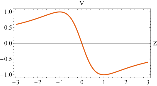
Figure 1: Initial condition

3 Case $s/2\in\mathbb{Z}$

The Hopf-Cole transformation [15, 13]

$$V=-\frac{2}{s}\frac{\partial}{\partial Z}\ln W$$ (5)

applied to (3) yields a diffusion equation

$$\frac{\partial W}{\partial T}=\frac{1}{s}\frac{\partial^{2}W}{\partial Z^{2}}.$$ (6)

The particular form (4) of the initial condition for $V$ allows it to escape the exponent in the initial condition for $W$

$$W(0,Z)=C\exp\left[-\frac{s}{2}\int V(0,Z)dZ\right]=C\exp\left[\frac{s}{2}\ln(1+Z^{2})\right]=C(1+Z^{2})^{s/2}.$$ (7)

The solution of (6) can be written in a standard form (for brevity $r=s/2$)

$$W(T,Z)=C\sqrt{\frac{r}{2\pi T}}\int_{-\infty}^{\infty}\exp[-\frac{r}{2T}(Z-\widehat{Z})^{2}](1+\widehat{Z}^{2})^{r}d\widehat{Z}.$$ (8)

If $r$ is integer the expression $(1+\widehat{Z}^{2})^{r}$ can be expanded using binomial coefficient

$$(1+\widehat{Z}^{2})^{r}=\sum_{\alpha=0}^{r}\binom{r}{\alpha}\widehat{Z}^{2\alpha},$$

and the solution $W(T,Z)$ breaks into a sum of integrals $I_{\alpha}$ (for breivity $\beta=r/T$)

$$W=\frac{C\sqrt{\beta}}{\sqrt{2\pi}}\sum_{\alpha=0}^{r}\binom{r}{\alpha}I_{\alpha}$$

$$I_{\alpha}=\int_{-\infty}^{\infty}\exp[-\frac{\beta}{2}(Z-\widehat{Z})^{2}]\widehat{Z}^{2\alpha}d\widehat{Z}.$$

Each integral is a polynomial in $Z^{2}$

$$I_{\alpha}=\frac{\sqrt{2\pi}}{\beta^{\alpha+1/2}}\frac{(2\alpha)!}{2^{\alpha}\alpha!}\sum_{k=0}^{\alpha}(-\beta Z^{2})^{k}\frac{(-\alpha)_{k}}{2^{k}k!(1/2)_{k}},$$

where $(a)_{b}\equiv a(a+1)(a+2)\ldots(a+b-1)$ is the Pochhammer symbol. Thus, $W$ can be written using double summation

$$W=C\sum_{\alpha=0}^{r}\left[\binom{r}{\alpha}\frac{(2\alpha)!}{2^{\alpha}\alpha!}\frac{1}{\beta^{\alpha}}\sum_{k=0}^{\alpha}(-\beta Z^{2})^{k}\frac{(-\alpha)_{k}}{2^{k}k!(1/2)_{k}}\right].$$ (9)

It is useful to separate $Z$ and $\beta$ by changing the order of summation

$$W=C\sum_{k=0}^{r}\left[\frac{(-1)^{k}Z^{2k}}{2^{k}k!(1/2)_{k}}\sum_{\alpha=k}^{r}\binom{r}{\alpha}\frac{(-\alpha)_{k}(2\alpha)!}{2^{\alpha}\alpha!}\left(\frac{1}{\beta}\right)^{\alpha-k}\right].$$

After substituting $\beta=r/T$, $r=s/2$ and simplifying the expression we obtain

$$W=C\sum_{k=0}^{s/2}\left[\frac{Z^{2k}}{2^{k}k!(2k-1)!!}\sum_{\alpha=k}^{s/2}\frac{(2\alpha)!}{\alpha!(s/2-\alpha)!(\alpha-k)!}\left(\frac{T}{s}\right)^{\alpha-k}\right].$$ (10)

Thus, $W$ is a polynomial of order $s/2$ in $Z^{2}$ and the coefficient of $(Z^{2})^{k}$ is a polynomial of order $s/2-k$ in $T$. According to (5), the relation between $V$ and $W$ is

$$V=-\frac{2}{s}\frac{\partial W/\partial Z}{W}.$$ (11)

Therefore, the solution of (3) for even $s$ is

$$V(s,T,Z)=-\frac{2}{s}\frac{\sum_{k=0}^{s/2}\left[\frac{Z^{2k-1}}{2^{k-1}(k-1)!(2k-1)!!}\sum_{\alpha=k}^{s/2}\frac{(2\alpha)!}{\alpha!(s/2-\alpha)!(\alpha-k)!}\left(\frac{T}{s}\right)^{\alpha-k}\right]}{\sum_{k=0}^{s/2}\left[\frac{Z^{2k}}{2^{k}k!(2k-1)!!}\sum_{\alpha=k}^{s/2}\frac{(2\alpha)!}{\alpha!(s/2-\alpha)!(\alpha-k)!}\left(\frac{T}{s}\right)^{\alpha-k}\right]}$$ (12)

It is worth noticing that for rational $T,Z$ this expression is also a rational number which can be useful for numerical applications.

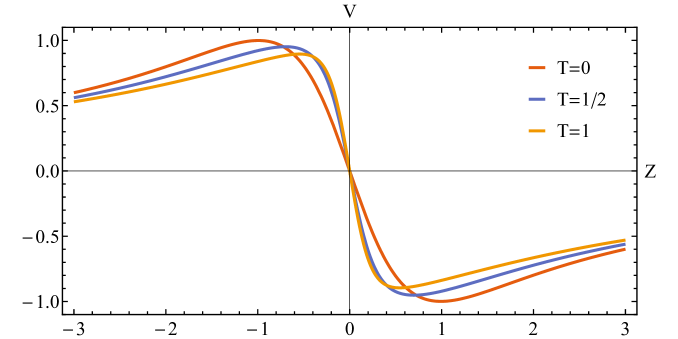
Figure 2: The solution of Burgers equation (1) for $s=10$

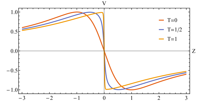
Figure 3: The solution of Burgers equation (1) for $s=100$

To use this solution for verification of numerical methods one can choose the $Z$ domain as an interval $[-A,A]$ and impose the boundary conditions using $\mp V(s,T,A)$. This expression is a rational function of $T$ and if $A\gg 1$ it has a slowly changing value close to zero.

4 Case $s=\infty$

The expression (12) obtained for a finite $s$ cannot be easily generalized for $s\rightarrow\infty$. We consider this case separately:

$$\frac{\partial V}{\partial T}+V\frac{\partial V}{\partial Z}=0,$$ (13)

$$V(0,Z)=-\frac{2Z}{1+Z^{2}}.$$

A well known implicit solution

$$V(T,Z)=f(Z-V(T,Z)T)$$ (14)

would satisfy (13) and the boundary condition $V(0,Z)=f(Z)$, therefore $f(Z)=-2Z/(1+Z^{2}).$ By substituting it into (14) we obtain a polynomial of the third degree in $V$. After introducing for brevity

$$\phi=Z-VT,$$ (15)

the equation is written as $-\phi^{3}+Z\phi^{2}+\phi(2T-1)+Z=0.$ Consider one of its roots

$$\phi_{1}(T,Z)=\frac{1}{3}\left(Z-\frac{Z^{2}+6T-3}{(B+3\sqrt{D})^{1/3}}-(B+3\sqrt{D})^{1/3}\right),$$

$$B=-Z(9+9T+Z^{2}),\quad D=3Z^{4}-3Z^{2}(T(T-10)-2)-3(2T-1)^{3}.$$

According to (15) the solution $V$ is

$$V=Z/T-\phi_{1}/T.$$ (16)

For $T<1/2$ it satisfies the equation at any $Z$. If $T=1/2$ and $Z=0$ the expression $D$ under the radical is zero. This corresponds to the wave tipping, the derivative $\partial V/\partial Z$ jumps to $-\infty$ (see Figure 4). For $T>1/2$, $D$ has a negative the sign in a certain neighborhood of $Z=0$, but one can still choose cubic roots properly so that $\phi_{1}$ will be a real number. One can construct a multivalued solution for $T>1/2$ by choosing all real roots among $\phi_{1},\phi_{2},\phi_{3}$.

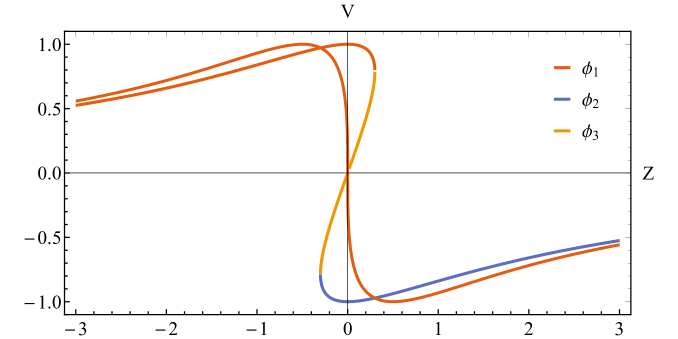
Figure 4: Invicid solution for $T=1/2$ and its multi-valued continuation for $T=1$.

To obtain the single-valued solution we use symmetry considerations. Namely, the initial condition and equation do not change under transformation $Z\rightarrow-Z$, $V\rightarrow-V$. Therefore, the solution should not either: $V(-Z,T)=-V(Z,T).$ The solution obtained with $\phi_{1}$ (orange curve on the Figure 4) is smooth for all $T$ if $Z<0$ and also satisfies the initial condition. By continuing it (anti)symmetrically for $Z>0$

$$\tilde{V}=\text{sign}(Z)\frac{|Z|+\phi_{1}(T,-|Z|)}{T}$$

we obtain a discontinuity at $Z=0$ for $T>1/2$. This is a stationary shock ($Z\equiv 0$), and in this case the Rankine-Hugonio condition is

$$V(+0,T)+V(-0,T)=0.$$

$\tilde{V}$ satisfies this relation, therefore it is a weak solution of the problem. One can observe that by comparing viscous solutions for large $s$ with $\tilde{V}$ for $T=1$ (see Figure 5).

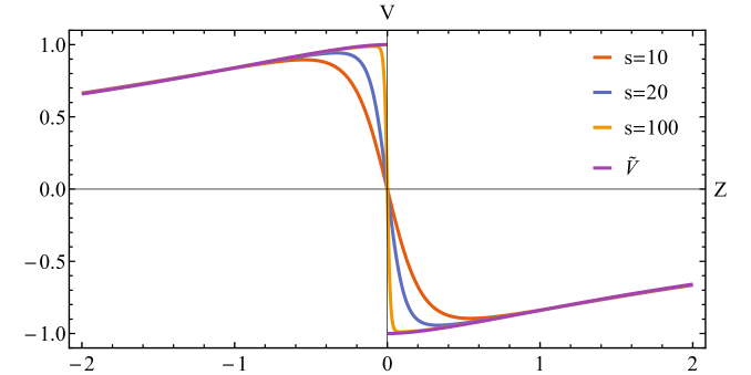
Figure 5: Smooth viscous solutions approaching discontinuous $\tilde{V}$ as the Reynolds number $s$ increases

5 Asymptotic for $s\rightarrow\infty$

5.1 Convergence to the invicid solution

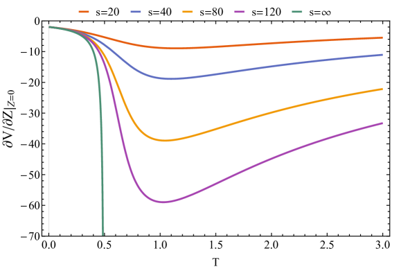
Figure 6: The slope of different solutions at the tipping point $Z=0$ for various $s$

After looking at Figure 6 one can notice that in contrast with the inviscid case, in which the derivative jumps to $-\infty$ at the tipping time $T=1/2$ and then the shock forms, the minimal derivative for large but finite $s$ occurs at $T\sim 1$ and is approximately $-s/2$. Let us inspect this value more carefully. By differentiating $V$ with respect to $Z$ and putting $Z=0$

$$\frac{\partial V}{\partial Z}=-\frac{2}{s}\frac{\partial}{\partial Z}\left(\frac{\partial W/\partial Z}{W}\right)\stackrel{{\scriptstyle Z\rightarrow 0}}{{=}}-\frac{2}{s}\left.\frac{\partial^{2}W/\partial Z^{2}}{W}\right|_{Z=0}$$

($W$ has only even powers of $Z$ therefore $\left.\partial W/\partial Z\right|_{Z=0}=0$). The denominator is the coefficient of $Z^{0}$ in (10), and the numerator is the doubled coefficient of $Z^{2}$. Luckily, the sum over $\alpha$ in (10) is expressed via Hypergeometric function:

$$\sum_{\alpha=k}^{s/2}\frac{(2\alpha)!}{\alpha!(\frac{s}{2}-\alpha)!(\alpha-k)!}\left(\frac{T}{s}\right)^{\alpha-k}=\frac{\left(s/T\right)^{k+1/2}\frac{s}{2}!}{2\sqrt{\pi}(\frac{s}{2}-k)!}\Gamma(\frac{1}{2}+k)U(\frac{1}{2}+k,\frac{3+s}{2},\frac{s}{4T})$$ (17)

$$U(a,c,z)=\frac{1}{\Gamma(a)}\int_{0}^{\infty}e^{-zt}t^{a-1}(1+t)^{c-a-1}dt$$

After substituting $k=0;1$ into (17), dividing by $2^{k}k!(2k-1)!!$ and simplifying, we obtain

$$\left.\frac{\partial V}{\partial Z}\right|_{Z=0}=-\frac{s}{2T}\frac{U(\frac{3}{2},\frac{3+s}{2},\frac{s}{4T})}{U(\frac{1}{2},\frac{3+s}{2},\frac{s}{4T})}.$$ (18)

At $s\rightarrow\infty$ the second and the third arguments of $U$ tend to infinity $c,z\rightarrow\infty$, and there are three different asymptotic depending on the ratio $z/c$. If $T<1/2$ then $z/c>1$, and the expansion according to [16] is

$$U(a,c,z)\sim(z-c)^{-a}\left(1+\frac{a(1+a)(c-2z)}{2(z-c)^{2}}+O\left(\frac{1}{c^{2}}\right)\right).$$

By substituting it into (18) and expanding the result, we obtain the asymptotic of the viscous slope for $T<1/2$

$$\left.\frac{\partial V}{\partial Z}\right|_{Z=0}\sim-\frac{2}{1-2T}+\frac{12T}{(1-2T)^{3}}\frac{1}{s}+O\left(\frac{1}{s^{2}}\right).$$ (19)

For the inviscid solution (16), unsurprisingly

$$\left.\frac{\partial V}{\partial Z}\right|_{Z=0}^{s=\infty}=-\frac{2}{1-2T}.$$ (20)

For $T<1/2$ at $Z=0$ viscous solutions are equal to the inviscid one, therefore the discrepancy between their slopes hints on the speed of convergence of the viscous solutions to the inviscid case (at least in a small neighborhood of $Z=0$) as the Reynolds number approaches infinity. However, expression (19) can not be used near the tipping time. At $T=1/2$ the proper expansion of $U$ at $c,z\rightarrow\infty$ is for which $z/c=1$

$$U(a,c,c)\sim\sqrt{\pi}(2c)^{-a/2}\left(\frac{1}{\Gamma((a+1)/2)}+O\left(\frac{1}{\sqrt{c}}\right)\right)\text{.}$$

Plugging it into (18) and expanding the result yields

$$\left.\frac{\partial V}{\partial Z}\right|_{Z=0;T=1/2}\sim-\frac{\Gamma(3/4)}{\Gamma(5/4)}\sqrt{s}+O(1)\simeq-1.35\sqrt{s}+O(1).$$ (21)

The gradient of the inviscid solution jumps to $-\infty$ and the viscous solution catches up with a speed proportional to $\sqrt{s}.$

5.2 Extremum of the gradient

Figure 3 suggests that the maximum slope occurs at $Z=0$. Indeed, at this line the equation turns into $\partial^{2}V/\partial Z^{2}=0$, so any point of it is critical for $\partial V/\partial Z$. To find the critical time $T_{\text{c}}$ consider the derivative of (18) with respect to $T$. It can be evaluated using the relation

$$\frac{\partial}{\partial z}U(a,c,z)=-a\cdot U(a+1,c+1,z),$$

and expanding the results. We expect $T_{\text{c}}>1/2$ therefore $z/c<1$, so the appropriate asymptotic of $U$ at $c,z\rightarrow\infty$ is

$$U(a,c,z)\sim\frac{\sqrt{2\pi}}{\Gamma(a)}c^{c-3/2}(1-z/c)^{a-1}\exp(z-c)\sum_{p=0}^{\infty}\frac{d_{p}}{c^{p}}$$ (22)

where $d_{0}=1$ and $d_{p}$ are described in [16]. Using three terms, we obtain

$$\frac{\partial}{\partial T}\left.\frac{\partial V}{\partial Z}\right|_{Z=0}\sim\frac{s(-1+T)}{T^{3}}+\frac{1-4T}{T^{2}(2T-1)^{2}}+O\left(\frac{1}{s}\right)=0.$$ (23)

Solving (23) for $T$ and expanding the result gives

$$T_{\text{c}}\sim 1+\frac{3}{s}+O\left(\frac{1}{s^{2}}\right).$$ (24)

By substituting (24) into (18) and expanding the result we obtain

$$\left.\frac{\partial V}{\partial Z}\right|_{Z=0;T=T_{\text{c}}}\sim-\frac{s}{2}+1+\frac{7}{2s}+O\left(\frac{1}{s^{2}}\right).$$

This gradient decreases much faster than the one at the moment of wave tipping (21). To evaluate the Hessian of the slope we obtain similarly:

$$\frac{\partial}{\partial Z^{2}}\left.\frac{\partial V}{\partial Z}\right|_{Z=0;T=T_{\text{c}}}\sim\frac{s^{3}}{4}-s^{2}-\frac{5s}{2}+O\left(1\right).$$

The mixed derivative $\partial^{2}/\partial Z\partial T$ of the slope is zero and $\partial^{2}/\partial T^{2}$ can be calculated directly from (23), and it is positive. Therefore the Hessian is positively defined for large enough $s$ and the point $Z=0$, $T=T_{c}$ is a local minimum.

6 Final remarks

We used the fact that the initial condition $V(0,Z)=-\partial/\partial Z\log[1+Z^{2}]=-2Z/(1+Z^{2})$ led to the factor $(1+\widehat{Z}^{2})^{s/2}$ in the integral with $d\widehat{Z}$ (8), and this factor can be expanded using binomial coefficient. Multinomial coefficients can expand powers of three and more summands, this allows to obtain physically viable rational solutions for the initial conditions of a form $V(0,Z)=-\partial/\partial Z\log[\sum_{l=0}^{2n}c_{l}Z^{l}]$, where $c_{l}$ ensure no real roots. In this general case, however, the inviscid solution cannot be expressed in radicals.

References

- [1] O. Rudenko, V. Gusev, Self-similar solutions of a burgers-type equation with quadratically cubic nonlinearity, in: Doklady Mathematics, Vol. 93, Springer, 2016, pp. 94–98.
- [2] J. M. Burgers, The nonlinear diffusion equation: asymptotic solutions and statistical problems, Springer Science & Business Media, 2013.
-
[3]
S. N. Gurbatov, A. I. Saichev, S. F. Shandarin,
Large-scale structure of the
universe. the zeldovich approximation and the adhesion model, Phys. Usp.
55 (3) (2012) 223–249.
doi:10.3367/UFNe.0182.201203a.0233.
URL https://ufn.ru/en/articles/2012/3/b/ - [4] E. R. Benton, G. W. Platzman, A table of solutions of the one-dimensional burgers equation, Quarterly of Applied Mathematics 30 (2) (1972) 195–212.
- [5] S. Dhawan, S. Kapoor, S. Kumar, S. Rawat, Contemporary review of techniques for the solution of nonlinear burgers equation, Journal of Computational Science 3 (5) (2012) 405–419.
- [6] N. A. Kudryashov, M. B. Soukharev, Comment on: Multi soliton solution, rational solution of the boussinesq–burgers equations, Communications in Nonlinear Science and Numerical Simulation 15 (7) (2010) 1765.
- [7] E. Y. Rodin, A riccati solution for burgers’ equation, Quarterly of Applied Mathematics 27 (4) (1970) 541–545.
- [8] E. Y. Rodin, On some approximate and exact solutions of boundary value problems for burgers’ equation, Journal of Mathematical Analysis and Applications 30 (2) (1970) 401–414.
- [9] A. V. Samokhin, The burgers equation with periodic boundary conditions on an interval, Theoretical and Mathematical Physics 188 (3) (2016) 1371–1376.
- [10] A.-M. Wazwaz, The variational iteration method for rational solutions for kdv, k (2, 2), burgers, and cubic boussinesq equations, Journal of Computational and Applied Mathematics 207 (1) (2007) 18–23.
- [11] W. Wood, An exact solution for burger’s equation, Communications in numerical methods in engineering 22 (7) (2006) 797–798.
- [12] D. Guzhev, N. N. Kalitkin, Burgers equation is a test for numerical methods, Matematicheskoe modelirovanie 7 (4) (1995) 99–127.
- [13] J. D. Cole, On a quasi-linear parabolic equation occurring in aerodynamics, Quarterly of applied mathematics 9 (3) (1951) 225–236.
- [14] C. Basdevant, M. Deville, P. Haldenwang, J. Lacroix, J. Ouazzani, R. Peyret, P. Orlandi, A. Patera, Spectral and finite difference solutions of the burgers equation, Computers & fluids 14 (1) (1986) 23–41.
- [15] E. Hopf, The partial differential equation ut+ uux= uxx, Communications on Pure and Applied mathematics 3 (3) (1950) 201–230.
- [16] N. M. Temme, Asymptotic methods for integrals, World Scientific Singapore, 2015.