Bayesian Optimization using Pseudo-Points

Abstract.

Bayesian optimization (BO) is a popular approach for expensive black-box optimization, with applications including parameter tuning, experimental design, robotics. BO usually models the objective function by a Gaussian process (GP), and iteratively samples the next data point by maximizing an acquisition function. In this paper, we propose a new general framework for BO by generating pseudo-points (i.e., data points whose objective values are not evaluated) to improve the GP model. With the classic acquisition function, i.e., upper confidence bound (UCB), we prove that the cumulative regret can be generally upper bounded. Experiments using UCB and other acquisition functions, i.e., probability of improvement (PI) and expectation of improvement (EI), on synthetic as well as real-world problems clearly show the advantage of generating pseudo-points.

1. Introduction

In real-world applications, we often need to solve an optimization problem:

$$\bm{x}^{*}\in\mathop{\arg\max}\nolimits_{\bm{x}\in\mathcal{X}}f(\bm{x}),$$

where $\mathcal{X}\subseteq\mathbb{R}^{d}$ is the solution space, $f:\mathcal{X}\rightarrow\mathbb{R}$ is the objective function, and $\bm{x}^{*}$ is a global optimal solution. Usually, it is assumed that $f$ has a known mathematical expression, is convex, or cheap to evaluate at least. Increasing evidences, however, show that $f$ may not satisfy these assumptions, but is an expensive black-box model (Brochu et al., 2010). That is, $f$ can be non-convex, or even the closed-form expression of $f$ is unknown; meanwhile, evaluating $f$ can be noisy and computationally very expensive.

Expensive black-box optimization is involved in many real-world decision making problems. For example, in machine learning, one has to tune hyper-parameters to maximize the performance of a learning algorithm (Snoek et al., 2012); in physical experiments, one needs to set proper parameters of the experimental environment to obtain an ideal product (Brochu et al., 2010). More applications can been found in robotic control (Martinez-Cantin et al., 2007), computer vision (Denil et al., 2012), sensor placing (Garnett et al., 2010), and analog circuit design (Lyu et al., 2018).

Bayesian optimization (BO) (Mockus, 1994) has been a type of powerful algorithm to solve expensive black-box optimization problems. The main idea is to build a model, usually by a Gaussian process (GP), for the objective function $f$ based on the observation data, and then sample the next data point by maximizing an acquisition function. Many BO algorithms have been proposed, with the goal of reaching the global optima using as few objective evaluations as possible.

Most existing works focus on designing effective acquisition functions, e.g., probability of improvement (PI) (Kushner, 1964), expectation of improvement (EI) (Jones et al., 1998), and upper confidence bound (UCB) (Srinivas et al., 2012). Recently, Wang et al. (Wang et al., 2016) proposed the EST function by directly estimating $\bm{x}^{*}$, which automatically and adaptively trades off exploration and exploitation in PI and UCB. Another major type of acquisition functions is based on information entropy, including entropy search (ES) (Hennig and Schuler, 2012), predictive ES (Hernández-Lobato et al., 2014), max-value ES (Wang and Jegelka, 2017), FITBO (Ru et al., 2018), etc. As BO is a sequential algorithm, some parallelization techniques have been introduced for acceleration, e.g., (Azimi et al., 2010; Desautels et al., 2014; Shah and Ghahramani, 2015; González et al., 2016). There is also a sequence of works addressing the difficulty of BO for high-dimensional optimization, e.g., (Wang et al., 2013; Kandasamy et al., 2015; Wang et al., 2017; Mutny and Krause, 2018).

For any BO algorithm with a specific acquisition function, the GP model becomes increasingly accurate with the observation data augmenting. However, the number of data points to be evaluated is often limited due to the expensive objective evaluation. In this paper, we propose a general framework for BO by generating pseudo-points to improve the GP model. That is, before maximizing the acquisition function to select the next point in each iteration, some pseudo-points are generated and added to update the GP model. The pseudo-points are neighbors of the observed data points, and take the same function values as the observed ones. Without increasing the evaluation cost, the generation of pseudo-points can reduce the variance of the GP model, while introducing little accuracy loss under the Lipschitz assumption. This framework is briefly called BO-PP.

Theoretically, we study the performance of BO-PP w.r.t. the acquisition function UCB, called UCB-PP. We prove a general upper bound of UCB-PP on the cumulative regret, i.e., $\sum^{T}_{t=1}(f(\bm{x}^{*})-f(\bm{x}_{t}))$, where $\bm{x}_{t}$ denotes the sampled point in the $t$-th iteration. It is shown to be a generalization of the known bound (Srinivas et al., 2012) of UCB.

Empirically, we compare BO-PP with BO on synthetic benchmark functions as well as real-world optimization problems. The acquisition functions UCB, PI and EI are selected. The results clearly show the excellent performance of BO-PP. The superiority of UCB-PP over UCB verifies our theoretical analysis, and that of PI-PP over PI and EI-PP over EI shows the applicability of the proposed framework of generating pseudo-points.

We start the rest of the paper by introducing some background on BO. We then present in three subsequent sections the proposed framework BO-PP, theoretical analysis and empirical study, respectively. The final section concludes the paper.

2. Background

The general framework of BO is shown in Algorithm 1. It sequentially optimizes some given objective function $f(\bm{x})$ with assumptions on a prior distribution, i.e., a probabilistic model, over $f(\bm{x})$. In each iteration, BO selects a point $\bm{x}$ by maximizing an acquisition function $acq(\cdot)$, evaluates its objective value $f(\bm{x})$, and updates the prior distribution with the new data point.

2.1. GPs

A GP (Rasmussen and Williams, 2006) is commonly used as the prior distribution, which regards the $f$ value at each data point as a random variable, and assumes that all of them satisfy a joint Gaussian distribution specified by the mean value function $m(\cdot)$ and the covariance function $k(\cdot,\cdot)$. For convenience, $m(\cdot)$ is set to zero. Assume that the objective evaluation is subject to i.i.d. additive Gaussian noise, i.e., $y=f(\bm{x})+\epsilon$, where $\epsilon\sim\mathcal{N}(0,\sigma^{2})$. Let $[t]$ denote the set $\{1,2,\ldots,t\}$.

Given an observation data $D_{t}=\{(\bm{x}_{i},y_{i})\}^{t}_{i=1}$, we can obtain the posterior mean

(1) $$\mu_{t}(\bm{x})=\bm{k}_{t}(\bm{x})^{\mathrm{T}}(\mathbf{K}_{t}+\sigma^{2}\mathbf{I})^{-1}\bm{y}_{1:t}$$

and the posterior variance

(2) $$\sigma^{2}_{t}(\bm{x})=k(\bm{x},\bm{x})-\bm{k}_{t}(\bm{x})^{\mathrm{T}}(\mathbf{K}_{t}+\sigma^{2}\mathbf{I})^{-1}\bm{k}_{t}(\bm{x}),$$

where $\bm{k}_{t}(\bm{x})=[k(\bm{x}_{i},\bm{x})]_{i=1}^{t}$, $\mathbf{K}_{t}=[k(\bm{x}_{i},\bm{x}_{j})]_{i,j\in[t]}$ and $\bm{y}_{1:t}=[y_{1};y_{2};\ldots;y_{t}]$. For a GP, the log likelihood of observed data $D_{t}$ is

$$\log\mathrm{Pr}(\bm{y}_{1:t}\mid\{\bm{x}_{i}\}^{t}_{i=1},\bm{\theta})=-\frac{1}{2}\bm{y}_{1:t}^{\mathrm{T}}(\mathbf{K}_{t}+\sigma^{2}\mathbf{I})^{-1}\bm{y}_{1:t}-\frac{1}{2}\log\mathrm{det}(\mathbf{K}_{t}+\sigma^{2}\mathbf{I})-\frac{t}{2}\log 2\pi,$$

where $\bm{\theta}$ denote the hyper-parameters of $k(\cdot,\cdot)$, and $\mathrm{det}(\cdot)$ denotes the determinant of a matrix. When updating the GP model in line 5 of Algorithm 1, the hyper-parameters $\bm{\theta}$ can be updated by maximizing the log likelihood of the augmented data, or treated to be fully Bayesian.

Algorithm 1 BO Framework

0:  iteration budget $T$

0:  

1:  let $D_{0}=\emptyset$;

2:  for $t=1:T$ do

3:     $\bm{x}_{t}=\arg\max_{\bm{x}\in\mathcal{X}}acq(\bm{x})$;

4:     evaluate $f$ at $\bm{x}_{t}$ to obtain $y_{t}$;

5:     augment the data $D_{t}=D_{t-1}\cup\{(\bm{x}_{t},y_{t})\}$ and update the GP model

6:  end for

2.2. Acquisition Functions

The data point to be evaluated in each iteration is selected by maximizing an acquisition function, which needs to trade off exploration, i.e., large posterior variances, and exploitation, i.e., large posterior means. Many acquisition functions have been proposed, and we introduce three typical ones, i.e., PI (Kushner, 1964), EI (Jones et al., 1998) and UCB (Srinivas et al., 2012), which will be examined in this paper.

Let $\bm{x}^{+}$ be the best point generated in the first $(t-1)$ iterations, and $Z=(\mu_{t-1}(\bm{x})-f(\bm{x}^{+}))/\sigma_{t-1}(\bm{x})$. Let $\Phi$ and $\phi$ denote the cumulative distribution and probability density functions of standard Gaussian distribution, respectively. PI selects the point by maximizing the probability of improvement, i.e.,

(3) $$\mathrm{PI}(\bm{x})=\mathrm{Pr}(f(\bm{x})>f(\bm{x}^{+}))=\Phi(Z).$$

EI selects the data point by maximizing the expectation of improvement, i.e.,

(4) $$\mathrm{EI}(\bm{x})=\left\{\begin{aligned} &(\mu_{t-1}(\bm{x})-f(\bm{x}^{+}))\Phi(Z)+\sigma_{t-1}(\bm{x})\phi(Z)&\text{if}\ \sigma_{t-1}(\bm{x})>0,\\ &0&\text{if}\ \sigma_{t-1}(\bm{x})=0.\end{aligned}\right.$$

UCB integrates the posterior mean and variance via a trade-off parameter $\beta_{t}$, i.e.,

(5) $$\mathrm{UCB}(\bm{x})=\mu_{t-1}(\bm{x})+\beta_{t}^{1/2}\sigma_{t-1}(\bm{x}),$$

and selects the data point by maximizing this measure.

2.3. Regrets

To evaluate the performance of BO algorithms, regrets are often used. The instantaneous regret $r_{t}=f(\bm{x}^{*})-f(\bm{x}_{t})$ measures the gap of function values between a global optimal solution $\bm{x}^{*}$ and the currently selected point $\bm{x}_{t}$. The simple regret $S_{T}=\min_{i\in[T]}r_{i}$ measures the gap between $\bm{x}^{*}$ and the best point found in the first $T$ iterations. The cumulative regret $R_{T}=\sum_{i=1}^{T}r_{i}$ is the sum of instantaneous regrets in the first $T$ iterations. It is clear that the simple regret $S_{T}$ is upper bounded by the average of the cumulative regret, i.e., $R_{T}/T$.

3. The BO-PP Framework

In BO, a GP is used to characterize the unknown objective function. The posterior variance of a GP describes the uncertainty about the unknown objective, while the posterior mean provides a closed form of the unknown objective. As the observation data augments, the posterior variance decreases and the posterior mean gets close to the unknown objective, making the GP express the unknown objective better. Thus, a straightforward way to improve the GP model is collecting more data points, which is, however, impractical, because the objective evaluation is expensive. In this section, we propose a general framework BO-PP by generating pseudo-points to improve the GP model.

As shown in Eq. (2), the posterior variance of $f$ does not depend on the objective values, and will be decreased by adding new data points. As shown in Eq. (1), the posterior mean of $f$ can be regarded as a linear combination of the observed objective values, and will be influenced by the error on the objective values of new data points. Inspired by the Lipschitz assumption, i.e., close data points have close objective values, the pseudo-points are selected to be neighbors of the observed data points, and take the same objective values as the observed ones.

The BO-PP framework is described in Algorithm 2. Before selecting the next data point in line 5, BO-PP generates a few pseudo-points to re-compute the posterior mean and variance of the GP model in lines 3-4, rather than directly using the GP model updated in the last iteration. After evaluating a new data point in line 6, the hyper-parameters of the covariance function employed by the GP model will be updated in line 7 using the truly observed data points by far. Note that the pseudo-points are only used to re-compute the posterior mean and variance.

Algorithm 2 BO-PP Framework

0:  iteration budget $T$

0:  $\{l_{i}\}^{T-1}_{i=0}$, $\{\tau_{i}\}^{T-1}_{i=0}$

0:  

1:  let $D_{0}=\emptyset$, $l_{0}=0$ and $\tau_{0}=0$;

2:  for $t=1:T$ do

3:     generate $l_{t-1}$ pseudo-points $\{(\bm{x}^{\prime}_{i},\hat{y}^{\prime}_{i})\}^{l_{t-1}}_{i=1}$;

4:     re-compute $\hat{\mu}_{t-1}$ and $\hat{\sigma}_{t-1}$ by $D_{t-1}\cup\{(\bm{x}^{\prime}_{i},\hat{y}^{\prime}_{i})\}^{l_{t-1}}_{i=1}$;

5:     $\bm{x}_{t}=\arg\max_{\bm{x}\in\mathcal{X}}acq(\bm{x})$;

6:     evaluate $f$ at $\bm{x}_{t}$ to obtain $y_{t}$;

7:     augment the data $D_{t}=D_{t-1}\cup\{(\bm{x}_{t},y_{t})\}$ and update the GP model

8:  end for

8:  where each pseudo-point in the $t$-th iteration has distance $\tau_{t-1}$ to some observed data point in $D_{t-1}$, and takes the same objective value as the observed one.

The way of generating pseudo-points can be diverse, e.g., randomly sampling a point with distance $\tau$ from some observed data point. The only requirement is that the pseudo-point takes the same objective value as the corresponding observed data point, which does not increase the evaluation cost. The number $l_{t}$ of pseudo-points and the distance $\tau_{t}$ employed in each iteration could affect the performance of the algorithm. For example, as $\tau_{t}$ decreases, the error on the objective values of pseudo-points will decrease, whereas the reduction on the posterior variance will also decrease. Their relationship will be analyzed in the theoretical analysis. Note that BO-PP can be equipped with any acquisition function.

4. Theoretical Analysis

In this section, we theoretically analyze the performance of BO-PP w.r.t. the acquisition function UCB, called UCB-PP. Specifically, we prove that the cumulative regret $R_{T}$ of UCB-PP can be generally upper bounded.

In the following analysis, let $\mu_{t}$ and $\sigma_{t}$ denote the posterior mean and variance after obtaining $D_{t}$; let $\hat{\mu}_{t}$ and $\hat{\sigma}_{t}$ denote the posterior mean and variance after adding pseudo-points $\{(\bm{x}^{\prime}_{i},\hat{y}^{\prime}_{i})\}^{l_{t}}_{i=1}$ into $D_{t}$; let $\tilde{\mu}_{t}$ and $\tilde{\sigma}_{t}$ denote the posterior mean and variance after adding pseudo-points with true observed values, i.e., $\{(\bm{x}^{\prime}_{i},y^{\prime}_{i}))\}^{l_{t}}_{i=1}$, where $y^{\prime}_{i}=f(\bm{x}^{\prime}_{i})+\epsilon^{\prime}_{i}$ with $\epsilon^{\prime}_{i}\sim\mathcal{N}(0,\sigma^{2})$. Some notations about pseudo-points: $\hat{\bm{y}}^{\prime}_{1:l_{t}}=[\hat{y}^{\prime}_{1};\hat{y}^{\prime}_{2};\ldots;\hat{y}^{\prime}_{l_{t}}]$; $\bm{y}^{\prime}_{1:l_{t}}=[y^{\prime}_{1};y^{\prime}_{2};\ldots;y^{\prime}_{l_{t}}]$; $\bm{k}^{\prime}_{l_{t}}(\bm{x})=[k(\bm{x}_{i}^{\prime},\bm{x})]^{l_{t}}_{i=1}$; $\mathbf{K}^{\prime}_{l_{t}}=[k(\bm{x}^{\prime}_{i},\bm{x}_{j}^{\prime})]_{i,j\in[l_{t}]}$; $\widetilde{\mathbf{K}}_{t,l_{t}}=[k(\bm{x}_{i},\bm{x}_{j}^{\prime})]_{i\in[t],j\in[l_{t}]}$; $\bm{p}(\bm{x})=\widetilde{\mathbf{K}}_{t,l_{t}}^{\mathrm{T}}(\mathbf{K}_{t}+\sigma^{2}\mathbf{I})^{-1}\bm{k}_{t}(\bm{x})-\bm{k}^{\prime}_{l_{t}}(\bm{x})$; $\mathbf{M}=(\mathbf{K}^{\prime}_{l_{t}}-\widetilde{\mathbf{K}}_{t,l_{t}}^{\mathrm{T}}(\mathbf{K}_{t}+\sigma^{2}\mathbf{I})^{-1}\widetilde{\mathbf{K}}_{t,l_{t}}+\sigma^{2}\mathbf{I})^{-1}$. For convenience of analysis, assume $k(\bm{x},\bm{x})=1$.

Let $A$ be a finite subset of $\mathcal{X}$, $\bm{f}_{A}$ denote their true objective values (which are actually random variables satisfying the posterior Gaussian distribution over the true objective values), and $\bm{y}_{A}$ denote the noisy observations. Let $PP$ denote all generated pseudo-points, and $\hat{\bm{y}}_{PP}$ denote their selected objective values. Note that $\hat{\bm{y}}_{PP}$ are random variables, as they are actually the noisy observation of the objective values of $PP$’s neighbor observed points. Let $\gamma^{\prime}_{T}=\max_{A:|A|=T}I(\bm{y}_{A};\bm{f}_{A})-\min_{A:|A|=T,PP}I(\bm{y}_{A};\hat{\bm{y}}_{PP})$, where $I(\cdot;\cdot)$ denotes the mutual information.

Theorem 1 gives an upper bound of UCB-PP on the cumulative regret $R_{T}$. As the analysis of UCB in (Srinivas et al., 2012), Assumption 1 is required, implying

(6) $$\mathrm{Pr}(\forall\bm{x},\bm{x}^{\prime}:|f(\bm{x})-f(\bm{x}^{\prime})|\leq L\|\bm{x}-\bm{x}^{\prime}\|_{1})\geq 1-dae^{-(L/b)^{2}}.$$

Assumption 1.

Suppose the kernel $k(\cdot,\cdot)$ satisfies the following high probability bound on the derivatives of $f$: for some constants $a,b>0$, $\forall j\in[d]:\mathrm{Pr}(sup_{\bm{x}\in\mathcal{X}}|\partial f/\partial x_{j}|>L)\leq ae^{-(L/b)^{2}}$.

Theorem 1.

Let $\mathcal{X}\subset[0,r]^{d}$, $\delta\in(0,1)$, and set $\beta_{t}$ in Eq. (5) as $\beta_{t}$$=2\log(2\pi^{2}t^{2}/(3\delta))+2d\log(t^{2}dbr\sqrt{\log(4da/\delta)})$. Running UCB-PP for $T$ iterations, it holds that

(7) $$\mathrm{Pr}\Big{(}R_{T}\leq\sqrt{CT\beta_{T}\gamma_{T}^{\prime}}+2+2\sum\nolimits_{t=1}^{T}\Delta_{m}(l_{t-1},\tau_{t-1})\Big{)}\geq 1-\delta,$$

where $C=8/\log(1+\sigma^{-2})$, and $\Delta_{m}(l_{t},\tau_{t})=l_{t}^{2}\sqrt{1+\sigma^{-2}}\Big{(}bd\tau_{t}\sqrt{\log(4da/\delta)}/\sigma+2\sqrt{\log\frac{4\sum\nolimits^{T-1}_{t=0}l_{t}}{\delta}}\Big{)}$.

Before giving the proof of Theorem 1, we first give some lemmas that will be used. Lemma 2 gives the reduction on the posterior variance by adding pseudo-points.

Lemma 0.

After obtaining $D_{t}$ in UCB-PP, the reduction on the posterior variance by adding pseudo-points $\{(\bm{x}^{\prime}_{i},\hat{y}^{\prime}_{i})\}^{l_{t}}_{i=1}$ is

(8) $$\Delta_{v}(\bm{x},l_{t},\tau_{t})=\sigma_{t}^{2}(\bm{x})-\hat{\sigma}^{2}_{t}(\bm{x})=\bm{p}(\bm{x})^{\mathrm{T}}\mathbf{M}\bm{p}(\bm{x}).$$

Proof.

By Eq. (2) and $k(\bm{x},\bm{x})=1$, we have

(9) $$\hat{\sigma}_{t}^{2}(x) =1-[\bm{k}_{t}(\bm{x});\bm{k}^{\prime}_{l_{t}}(\bm{x})]^{\mathrm{T}}\left(\left[\begin{matrix}\mathbf{K}_{t}&\widetilde{\mathbf{K}}_{t,l_{t}}\\ \widetilde{\mathbf{K}}_{t,l_{t}}^{\mathrm{T}}&\ \mathbf{K}^{\prime}_{l_{t}}\end{matrix}\right]+\sigma^{2}\mathbf{I}\right)^{-1}[\bm{k}_{t}(\bm{x});\bm{k}^{\prime}_{l_{t}}(\bm{x})]$$

$$=1-\bm{k}_{t}(\bm{x})^{\mathrm{T}}(\mathbf{K}_{t}+\sigma^{2}\mathbf{I})^{-1}\bm{k}_{t}(\bm{x})-\bm{p}(\bm{x})^{\mathrm{T}}\mathbf{M}\bm{p}(\bm{x})$$

$$=\sigma_{t}^{2}(\bm{x})-\bm{p}(\bm{x})^{\mathrm{T}}\mathbf{M}\bm{p}(\bm{x}),$$

where the second equality is derived by the inverse of a block matrix, and the third one holds by Eq. (2). Thus, the lemma holds. ∎

Lemma 3 is extracted from Lemma 5.1 in (Srinivas et al., 2012), and will be used in the proof of Lemma 4.

Lemma 0.

Suppose $X$ is a random variable satisfying the Gaussian distribution $\mathcal{N}(\mu,\sigma^{2})$. Then, it holds that

(10) $$\mathrm{Pr}(|X-\mu|>c\sigma)\leq e^{-c^{2}/2},$$

where $c>0$.

The error on the posterior mean led by the incorrect objective values of pseudo-points can be bounded as follows.

Lemma 0.

After obtaining $D_{t}$ in UCB-PP, the difference on the posterior mean by adding pseudo-points, i.e., $\{(\bm{x}^{\prime}_{i},\hat{y}^{\prime}_{i})\}^{l_{t}}_{i=1}$, and that with true observed values, i.e., $\{(\bm{x}^{\prime}_{i},y^{\prime}_{i}))\}^{l_{t}}_{i=1}$, is $\hat{\mu}_{t}(\bm{x})-\tilde{\mu}_{t}(\bm{x})=-\bm{p}(\bm{x})^{\mathrm{T}}\mathbf{M}(\hat{\bm{y}}^{\prime}_{1:l_{t}}-\bm{y}^{\prime}_{1:l_{t}})$. Furthermore, it holds that

(11) $$\mathrm{Pr}\left(\forall 0\leq t\leq T-1,\forall\bm{x}\in\mathcal{X}:|\hat{\mu}_{t}(\bm{x})-\tilde{\mu}_{t}(\bm{x})|\leq\Delta_{m}(L,l_{t},\tau_{t})\right)\geq 1-dae^{-(L/b)^{2}}-\delta/4,$$

where $\Delta_{m}(L,l_{t},\tau_{t})=l_{t}^{2}\sqrt{1+\sigma^{-2}}\Big{(}Ld\tau_{t}/\sigma+2\sqrt{\log\frac{4\sum\nolimits^{T-1}_{t=0}l_{t}}{\delta}}\Big{)}$.

Proof.

By Eq. (1), we have

(12) $$\hat{\mu}_{t}(\bm{x}) =[\bm{k}_{t}(\bm{x});\bm{k}^{\prime}_{l_{t}}(\bm{x})]^{\mathrm{T}}\left(\left[\begin{matrix}\mathbf{K}_{t}&\widetilde{\mathbf{K}}_{t,l_{t}}\\ \widetilde{\mathbf{K}}_{t,l_{t}}^{\mathrm{T}}&\mathbf{K}^{\prime}_{l_{t}}\end{matrix}\right]+\sigma^{2}\mathbf{I}\right)^{-1}[\bm{y}_{1:t};\hat{\bm{y}}_{1:l_{t}}^{\prime}]$$

(13) $$=\bm{k}_{t}(\bm{x})^{\mathrm{T}}(\mathbf{K}_{t}+\sigma^{2}\mathbf{I})^{-1}\bm{y}_{1:t}+\bm{p}(\bm{x})^{\mathrm{T}}\mathbf{M}([\mu_{t}(\bm{x}^{\prime}_{1});\mu_{t}(\bm{x}^{\prime}_{2});\ldots;\mu_{t}(\bm{x}^{\prime}_{l_{t}})]-\hat{\bm{y}}^{\prime}_{1:l_{t}})$$

(14) $$=\mu_{t}(\bm{x})+\bm{p}(\bm{x})^{\mathrm{T}}\mathbf{M}([\mu_{t}(\bm{x}^{\prime}_{1});\mu_{t}(\bm{x}^{\prime}_{2});\ldots;\mu_{t}(\bm{x}^{\prime}_{l_{t}})]-\hat{\bm{y}}^{\prime}_{1:l_{t}}),$$

where the second equality is derived by the inverse of a block matrix, and the third one holds by Eq. (1). Similarly, we have

(15) $$\tilde{\mu}_{t}(\bm{x}) =\mu_{t}(\bm{x})+\bm{p}(\bm{x})^{\mathrm{T}}\mathbf{M}([\mu_{t}(\bm{x}^{\prime}_{1});\mu_{t}(\bm{x}^{\prime}_{2});\ldots;\mu_{t}(\bm{x}^{\prime}_{l_{t}})]-\bm{y}^{\prime}_{1:l_{t}}).$$

Thus, it holds that $\hat{\mu}_{t}(\bm{x})-\tilde{\mu}_{t}(\bm{x})=-\bm{p}(\bm{x})^{\mathrm{T}}\mathbf{M}(\hat{\bm{y}}^{\prime}_{1:l_{t}}-\bm{y}^{\prime}_{1:l_{t}})$.

Next, we examine the upper bound on $|\bm{p}(\bm{x})^{\mathrm{T}}\mathbf{M}(\hat{\bm{y}}^{\prime}_{1:l_{t}}-\bm{y}^{\prime}_{1:l_{t}})|$.

(16) $$|\bm{p}(\bm{x})^{\mathrm{T}}\mathbf{M}(\hat{\bm{y}}^{\prime}_{1:l_{t}}-\bm{y}^{\prime}_{1:l_{t}})|\leq\sum_{i=1}^{l_{t}}|(\bm{p}(\bm{x})^{\mathrm{T}}\mathbf{M})_{i}|\cdot|\hat{y}_{i}^{\prime}-y^{\prime}_{i}|,$$

where $(\bm{p}(\bm{x})^{\mathrm{T}}\mathbf{M})_{i}$ denotes the $i$-th element of $\bm{p}(\bm{x})^{\mathrm{T}}\mathbf{M}$. According to the procedure of Algorithm 2, the pseudo-point $\bm{x}^{\prime}_{i}$ has distance $\tau_{t}$ with some observed data point and takes the same function value. Assume that the corresponding observed data point for $\bm{x}^{\prime}_{i}$ is $\bm{x}_{j}$, where $j\in[t]$, implying $\hat{y}^{\prime}_{i}=y_{j}$. Thus, we have

(17) $$|\hat{y}_{i}^{\prime}-y^{\prime}_{i}|=|y_{j}-y^{\prime}_{i}|=|(f(\bm{x}_{j})+\epsilon_{j})-(f(\bm{x}^{\prime}_{i})+\epsilon^{\prime}_{i})|\leq|f(\bm{x}_{j})-f(\bm{x}^{\prime}_{i})|+|\epsilon_{j}-\epsilon^{\prime}_{i}|,$$

where $\epsilon_{j},\epsilon^{\prime}_{i}\sim\mathcal{N}(0,\sigma^{2})$, and the second equality holds because $f(\bm{x}_{j})$ and $f(\bm{x}^{\prime}_{i})$ are subject to additive Gaussian noise $\mathcal{N}(0,\sigma^{2})$. According to Assumption 1, we have

(18) $$\mathrm{Pr}\left(\forall t\geq 0,\forall i\in[l_{t}]:|f(\bm{x}_{j})-f(\bm{x}^{\prime}_{i})|\leq L\|\bm{x}_{j}-\bm{x}^{\prime}_{i}\|_{1}=Ld\tau_{t}\right)\geq 1-dae^{-(L/b)^{2}}.$$

As $\epsilon_{j}-\epsilon^{\prime}_{i}\sim\mathcal{N}(0,2\sigma^{2})$, by Lemma 3, we have

(19) $$\mathrm{Pr}\left(|\epsilon_{j}-\epsilon^{\prime}_{i}|\leq 2\sigma\sqrt{\log\frac{4\sum\nolimits^{T-1}_{t=0}l_{t}}{\delta}}\right)\geq 1-\frac{\delta}{4\sum\nolimits^{T-1}_{t=0}l_{t}}.$$

Applying the union bound leads to

(20) $$\mathrm{Pr}\left(\forall 0\leq t\leq T-1,\forall i\in[l_{t}]:|\hat{y_{i}}^{\prime}-y^{\prime}_{i}|\leq Ld\tau_{t}+2\sigma\sqrt{\log\frac{4\sum\nolimits^{T-1}_{t=0}l_{t}}{\delta}}\right)$$

(21) $$\quad\geq 1-dae^{-(L/b)^{2}}-\left(\sum^{T-1}_{t=0}l_{t}\right)\cdot\frac{\delta}{4\sum^{T-1}_{t=0}l_{t}}\geq 1-dae^{-(L/b)^{2}}-\frac{\delta}{4}.$$

Thus, with probability at least $1-dae^{-(L/b)^{2}}-\delta/4$, it holds that $\forall 0\leq t\leq T-1$,

(22) $$|\bm{p}(\bm{x})^{\mathrm{T}}\mathbf{M}(\hat{\bm{y}}^{\prime}_{1:l_{t}}-\bm{y}^{\prime}_{1:l_{t}})| \leq\left(Ld\tau_{t}+2\sigma\sqrt{\log\frac{4\sum\nolimits^{T-1}_{t=0}l_{t}}{\delta}}\right)\sum_{i=1}^{l_{t}}|(\bm{p}(\bm{x})^{\mathrm{T}}\mathbf{M})_{i}|.$$

Next we prove an upper bound on $\sum_{i=1}^{l_{t}}|(\bm{p}(\bm{x})^{\mathrm{T}}\mathbf{M})_{i}|$. Note that

(23) $$|(\bm{p}(\bm{x})^{\mathrm{T}}\mathbf{M})_{i}|\leq\sum^{l_{t}}_{j=1}|\bm{p}(\bm{x})_{j}|\cdot|\mathbf{M}_{j,i}|,$$

where $\bm{p}(\bm{x})_{j}$ denotes the $j$-th element of $\bm{p}(\bm{x})$, and $\mathbf{M}_{j,i}$ denotes the element of the $j$-th row and $i$-th column of $\mathbf{M}$. If only one pseudo-point $(\bm{x}^{\prime}_{j},\hat{y}^{\prime}_{j})$ from $\{(\bm{x}^{\prime}_{i},\hat{y}^{\prime}_{i})\}^{l_{t}}_{i=1}$ is added into $D_{t}$, we know from Lemma 2 that the reduction on the posterior variance is

(24) $$\Delta_{v}(\bm{x},1,\tau_{t})=(\sigma_{t}^{2}(\bm{x}^{\prime}_{j})+\sigma^{2})^{-1}\bm{p}(\bm{x})_{j}^{2}\leq 1,$$

where the inequality holds by $k(\bm{x},\bm{x})=1$. This implies

(25) $$\forall j\in[l_{t}]:|\bm{p}(\bm{x})_{j}|\leq\sqrt{\sigma_{t}^{2}(\bm{x}^{\prime}_{j})+\sigma^{2}}\leq\sqrt{1+\sigma^{2}}.$$

Let $\mathrm{adj}(\cdot)$ denote the adjugate matrix, $[\cdot]_{i,j}$ denote the principle submatrix by deleting the $i$-th row and $j$-th column, and $\lambda_{k}(\cdot)$ denote the $k$-th largest eigenvalue. By Cramer’s rule, $\mathbf{M}=\mathrm{adj}(\mathbf{M}^{-1})/\mathrm{det}(\mathbf{M}^{-1})$, and thus,

(26) $$|\mathbf{M}_{j,i}|=|\mathrm{adj}(\mathbf{M}^{-1})_{j,i}|/\mathrm{det}(\mathbf{M}^{-1}) =\mathrm{det}([\mathbf{M}^{-1}]_{i,j})/\mathrm{det}(\mathbf{M}^{-1})$$

(27) $$=\prod_{k=1}^{l_{t}-1}\lambda_{k}([\mathbf{M}^{-1}]_{i,j})/\prod_{k=1}^{l_{t}}\lambda_{k}(\mathbf{M}^{-1})$$

(28) $$\leq 1/\lambda_{l_{t}}(\mathbf{M}^{-1})\leq\sigma^{-2},$$

where the second equality holds by the definition of the adjugate matrix, and the two inequalities hold by the Cauchy interlacing inequality, leading to $\lambda_{1}(\mathbf{M}^{-1})\geq\lambda_{1}([\mathbf{M}^{-1}]_{i,j})\geq\cdots\geq\lambda_{l_{t}-1}(\mathbf{M}^{-1})\geq\lambda_{l_{t}-1}([\mathbf{M}^{-1}]_{i,j})\geq\lambda_{l_{t}}(\mathbf{M}^{-1})\geq\sigma^{2}$. Combining Eqs. (23), (25) and (26), we have

(29) $$\sum_{i=1}^{l_{t}}|(\bm{p}(\bm{x})^{\mathrm{T}}\mathbf{M})_{i}|\leq\sum_{i=1}^{l_{t}}\sum_{j=1}^{l_{t}}|\bm{p}(\bm{x})_{j}|\cdot|\mathbf{M}_{j,i}|\leq\sqrt{1+\sigma^{2}}\sigma^{-2}l_{t}^{2}.$$

Applying Eq. (29) to Eq. (22), we have

(30) $$\mathrm{Pr}\Big{(}\forall 0\leq t\leq T-1,\forall\bm{x}\in\mathcal{X}:|\bm{p}(\bm{x})^{\mathrm{T}}\mathbf{M}(\hat{\bm{y}}^{\prime}_{1:l_{t}}-\bm{y}^{\prime}_{1:l_{t}})|$$

$$\qquad\leq\left(Ld\tau_{t}+2\sigma\sqrt{\log\frac{4\sum\nolimits^{T-1}_{t=0}l_{t}}{\delta}}\right)\sqrt{1+\sigma^{2}}\sigma^{-2}l_{t}^{2}\Big{)}\geq 1-dae^{-(L/b)^{2}}-\delta/4.$$

Thus, the lemma holds. ∎

The proof of Theorem 1 is inspired by that of Theorem 2 in (Srinivas et al., 2012), which gives an upper bound of UCB on the cumulative regret $R_{T}$. Their proof intuition is mainly that the instantaneous regret $r_{t}$ can be upper bounded by the width of confidence interval of $f(\bm{x}_{t})$, relating to the posterior variance. The generation of pseudo-points will introduce another quantity into the upper bound on $r_{t}$, characterized by the error on the posterior mean in Lemma 4.

Proof of Theorem 1.  According to Assumption 1 and $\beta_{t}=2\log(2\pi^{2}t^{2}(dt^{2}rL)^{d}/(3\delta))$, where $L=b\sqrt{\log(4da/\delta)}$, we can apply Lemma 5.7 in (Srinivas et al., 2012) to derive that

(31) $$\mathrm{Pr}(\forall t\geq 1:|f(\bm{x}^{*})-\tilde{\mu}_{t-1}([\bm{x}^{*}]_{t})|\leq\beta_{t}^{1/2}\tilde{\sigma}_{t-1}([\bm{x}^{*}]_{t})+1/t^{2})\geq 1-\delta/2,$$

where $[\bm{x}^{*}]_{t}$ denotes the discretized data point closest to $\bm{x}^{*}$ in the $t$-th iteration. Note that $\Delta_{m}(l_{t},\tau_{t})$ is just $\Delta_{m}(L,l_{t},\tau_{t})$ with $L=b\sqrt{\log(4da/\delta)}$ in Lemma 4. By the definition of $r_{t}$, we have

(32) $$\forall t\geq 1:r_{t} =f(\bm{x}^{*})-f(\bm{x}_{t})$$

(33) $$\leq\beta_{t}^{1/2}\tilde{\sigma}_{t-1}([\bm{x}^{*}]_{t})+\tilde{\mu}_{t-1}([\bm{x}^{*}]_{t})-f(\bm{x}_{t})+1/t^{2}$$

(34) $$\leq\beta_{t}^{1/2}\tilde{\sigma}_{t-1}([\bm{x}^{*}]_{t})+\hat{\mu}_{t-1}([\bm{x}^{*}]_{t})-f(\bm{x}_{t})+1/t^{2}+\Delta_{m}(l_{t-1},\tau_{t-1})$$

(35) $$=\beta_{t}^{1/2}\hat{\sigma}_{t-1}([\bm{x}^{*}]_{t})+\hat{\mu}_{t-1}([\bm{x}^{*}]_{t})-f(\bm{x}_{t})+1/t^{2}+\Delta_{m}(l_{t-1},\tau_{t-1})$$

(36) $$\leq\beta_{t}^{1/2}\hat{\sigma}_{t-1}(\bm{x}_{t})+\hat{\mu}_{t-1}(\bm{x}_{t})-f(\bm{x}_{t})+1/t^{2}+\Delta_{m}(l_{t-1},\tau_{t-1})$$

(37) $$\leq\beta_{t}^{1/2}\hat{\sigma}_{t-1}(\bm{x}_{t})+\tilde{\mu}_{t-1}(\bm{x}_{t})-f(\bm{x}_{t})+1/t^{2}+2\Delta_{m}(l_{t-1},\tau_{t-1})$$

(38) $$\leq 2\beta_{t}^{1/2}\hat{\sigma}_{t-1}(\bm{x}_{t})+1/t^{2}+2\Delta_{m}(l_{t-1},\tau_{t-1}),$$

where the first inequality holds with probability at least $1-\delta/2$ by Eq. (31), the second and fourth inequalities hold with probability at least $1-dae^{-(L/b)^{2}}-\delta/4=1-\delta/2$ by Lemma 4, the equality holds by $\forall\bm{x}:\hat{\sigma}_{t-1}(\bm{x})=\tilde{\sigma}_{t-1}(\bm{x})$, the third inequality holds because $\bm{x}_{t}$ is selected by maximizing $\hat{\mu}_{t-1}(\bm{x})+\beta_{t}^{1/2}\hat{\sigma}_{t-1}(\bm{x})$ in Eq. (5), and the last inequality holds with probability at least $1-\delta/4$ by Lemma 5.5 in (Srinivas et al., 2012). Note that to prove Lemma 5.7 in (Srinivas et al., 2012) and Lemma 4, Assumption 1, i.e., Eq. (6), is both used; thus, the probability $dae^{-(L/b)^{2}}=\delta/4$ has been repeated. By the union bound, we have

(39) $$\mathrm{Pr}(\forall t\geq 1:r_{t}\leq 2\beta_{t}^{1/2}\hat{\sigma}_{t-1}(\bm{x}_{t})+1/t^{2}+2\Delta_{m}(l_{t-1},\tau_{t-1}))\geq 1-\delta/2-\delta/4-\delta/4=1-\delta,$$

implying

(40) $$\qquad\;\mathrm{Pr}\Big{(}R_{T}=\sum\nolimits_{t=1}^{T}r_{t}\leq\sum\nolimits^{T}_{t=1}(2\beta_{t}^{1/2}\hat{\sigma}_{t-1}(\bm{x}_{t})+1/t^{2}+2\Delta_{m}(l_{t-1},\tau_{t-1}))\Big{)}\geq 1-\delta.$$

By the Cauchy–Schwarz inequality, $C=8/\log(1+\sigma^{-2})$ and $\forall t\leq T:\beta_{t}\leq\beta_{T}$, we have

(41) $$\sum\nolimits_{t=1}^{T}2\beta_{t}^{1/2}\hat{\sigma}_{t-1}(\bm{x}_{t}) \leq\sqrt{T\sum\nolimits_{t=1}^{T}4\beta_{t}\hat{\sigma}^{2}_{t-1}(\bm{x}_{t})}$$

(42) $$\leq\sqrt{\frac{CT\beta_{T}}{2}\sum\nolimits_{t=1}^{T}\log(1+\sigma^{-2}\hat{\sigma}^{2}_{t-1}(\bm{x}_{t}))}.$$

Let $PP_{t}$ denote the pseudo-points generated in the $t$-th iteration, and $\hat{\bm{y}}_{PP_{t}}$ denote their selected objective values. Let $H(\cdot)$ denote the entropy. We have

(43) $$\frac{1}{2}\sum\limits_{t=1}^{T}\log(1+\sigma^{-2}\hat{\sigma}^{2}_{t-1}(\bm{x}_{t}))+H(\bm{y}_{1:T}|\bm{f}_{1:T})$$

$$=\frac{1}{2}\sum\limits_{t=1}^{T}\log(1+\sigma^{-2}\hat{\sigma}^{2}_{t-1}(\bm{x}_{t}))+\frac{1}{2}\log(\det(2\pi e\sigma^{2}\mathbf{I}))$$

$$=\frac{1}{2}\sum\limits_{t=1}^{T}\log(2\pi e(\sigma^{2}+\hat{\sigma}^{2}_{t-1}(\bm{x}_{t})))$$

$$=H(y_{1}\mid\hat{\bm{y}}_{PP_{1}})+H(y_{2}\mid y_{1},\hat{\bm{y}}_{PP_{2}})+\cdots+H(y_{T}\mid\bm{y}_{1:T-1},\hat{\bm{y}}_{PP_{T}})$$

$$=H(y_{1}\mid\hat{\bm{y}}_{PP})+H(y_{2}\mid y_{1},\hat{\bm{y}}_{PP})+\cdots+H(y_{T}\mid\bm{y}_{1:T-1},\hat{\bm{y}}_{PP})$$

$$=H(\bm{y}_{1:T}\mid\hat{\bm{y}}_{PP}),$$

where the first equality holds because $f(\bm{x})$ is subject to additive Gaussian noise $\mathcal{N}(0,\sigma^{2})$. Thus,

(44) $$\frac{1}{2}\sum\limits_{t=1}^{T}\log(1+\sigma^{-2}\hat{\sigma}^{2}_{t-1}(\bm{x}_{t})) =H(\bm{y}_{1:T}\mid\hat{\bm{y}}_{PP})-H(\bm{y}_{1:T}\mid\bm{f}_{1:T})$$

(45) $$=H(\hat{\bm{y}}_{PP}\mid\bm{y}_{1:T})-H(\hat{\bm{y}}_{PP})+H(\bm{y}_{1:T})-H(\bm{y}_{1:T}\mid\bm{f}_{1:T})$$

(46) $$=I(\bm{y}_{1:T};\bm{f}_{1:T})-I(\bm{y}_{1:T};\hat{\bm{y}}_{PP})$$

(47) $$\leq\gamma^{\prime}_{T}.$$

Considering $\sum_{t\geq 1}1/t^{2}=\pi^{2}/6<2$, Eq. (7) holds. Thus, the theorem holds. $\square$

Under the same assumption, it has been proved (Srinivas et al., 2012) that the cumulative regret $R_{T}$ of UCB satisfies

(48) $$\mathrm{Pr}\big{(}R_{T}\leq\sqrt{CT\beta_{T}\gamma_{T}}+2\big{)}\geq 1-\delta,$$

where $\gamma_{T}=\max_{A:|A|=T}I(\bm{y}_{A};\bm{f}_{A})$, and the other parameters have the same meaning as that in Theorem 1. Our bound on $R_{T}$ of UCB-PP is actually a generalization of that of UCB. Without generating pseudo-points, $\forall t\geq 0:l_{t}=0\wedge I(\bm{y}_{A};\hat{\bm{y}}_{PP})=0$, and thus, $\gamma^{\prime}_{T}=\gamma_{T}\wedge\Delta_{m}(l_{t},\tau_{t})=0$, implying that Eq. (7) specializes to Eq. (48). As $\gamma^{\prime}_{T}\leq\gamma_{T}$, the comparison between Eqs. (7) and (48) suggests that the generation of pseudo-points can be helpful if the negative influence of introducing the error on the posterior mean, i.e., introducing the term $\Delta_{m}(l_{t},\tau_{t})$, can be compensated by the positive influence of reducing the posterior variance, i.e., introducing the term $I(\bm{y}_{1:T};\hat{\bm{y}}_{PP})$.

5. Empirical Study

In this section, we empirically compare BO-PP with BO. Three common acquisition functions, i.e., UCB, PI and EI, are used. The ARD squared exponential kernel is employed, whose hyper-parameters are tuned by maximum likelihood estimation (MLE), and the acquisition function is maximized via the DIRECT algorithm (Jones et al., 1993). To alleviate the “cold start” issue, each algorithm starts with five random initial points. To compare BO-PP with BO on each problem, we repeat their running 20 times independently and report the average results; in each running, BO-PP and BO use the same five random initial points. The noise level is set to $\sigma^{2}=0.0001$, and the iteration budget is set to 100.

In the $(t+1)$-th iteration of BO-PP, for each point in $D_{t}$, one pseudo-point is generated by randomly sampling within its distance $\tau_{t}$ and taking the same function value; thus, $l_{t}=|D_{t}|$. To control the error of objective values with pseudo-points increasing, $\tau_{t}$ is set to $r\tau_{0}/(dl_{t})$, which decreases with $l_{t}$. Note that $r$ corresponds to the width of each dimension of the search domain. $\tau_{0}$ is set to a small value. We will use 0.01, 0.001 and 0.0001 to explore its influence, and the corresponding algorithms are denoted as BO-PP01, BO-PP001 and BO-PP0001, respectively.

We use four common synthetic benchmark functions: Dropwave, Griewank, Hart6 and Rastrigin, whose dimensions are 2, 2, 6 and 2, respectively. Their search domains are scaled to $[-1,1]^{d}$. As the global minima are known, the simple regret $S_{T}$ is used as the metric. We also employ four real-world optimization problems, widely used in BO experiments (Springenberg et al., 2016; Wang and Jegelka, 2017; Ru et al., 2018). The first is to tune the hyper-parameters, i.e., box constraint $C\in[0.001,1000]$ and kernel scale $l\in[0.0001,1]$, of SVM for classification on the data set Wine quality (1,599 #inst, 11 #feat). The second is to tune the hyper-parameters of 1-hidden-layer neural network (NN) for this task. The NN is trained by backpropagation, and the hyper-parameters are the number of neurons $n\in[1,100]$ and the learning rate $l_{r}\in[0.000001,1]$. The last two problems are to tune the hyper-parameters of 1-hidden-layer NN for classification on Breast cancer (699 #inst, 9 #feat) and regression on Boston housing (506 #inst, 13 #feat), respectively. The NN is trained by Levenberg-Marquardt optimization, and there are four hyper-parameters: $n\in[1,100]$, the damping factor $\mu\in[0.000001,100]$, the $\mu$-decrease and $\mu$-increase factors $\mu_{dec}\in[0.01,1]$, $\mu_{inc}\in[1.01,20]$. All data sets are randomly split into training/validation/test sets with ratio 0.7/0.2/0.1, and the performance on validation sets is used as the objective $f$. For classification, $f$ is the classification accuracy; for regression, $f$ equals 20 minus the regression L2-loss. All codes and data sets can be downloaded from https://github.com/TELO19/BOPP.

For UCB, $\beta_{t}$ in Eq. (5) is set to $2\log(t^{d/2+2}\pi^{2}/3\delta)$ where $\delta=0.1$, as suggested in (Brochu et al., 2010; Srinivas et al., 2012). For PI and EI, the best observed function value by far is used as $f(\bm{x}^{+})$ in Eqs. (3) and (4). The results are summarized in Table 1. We can observe that UCB-PP0001 is always better than UCB, verifying our theoretical analysis; UCB-PP01 and UCB-PP001 surpass UCB in most cases, disclosing that the performance of UCB-PP is not very sensitive to the distance $\tau_{t}$. Also, PI-PP and EI-PP perform better than PI and EI, respectively, in most cases, showing the applicability of generating pseudo-points.

Table 1. The results (mean$\pm$std.) of BO-PP and BO on synthetic benchmark functions and real-world optimization problems, when reaching the iteration budget. $S_{T}$: the smaller, the better; $f$: the larger, the better. The bolded values denote that BO-PP is no worse than BO. UCB, PI and EI are tested.

Function		UCB	UCB-PP01	UCB-PP001	UCB-PP0001
$S_{T}$	Dropwave	0.2710$\pm$0.1311	0.2232$\pm$0.1053	0.1630$\pm$0.1014	0.2121$\pm$0.1038
	Griewank	0.2357$\pm$0.2125	0.2272$\pm$0.1644	0.2350$\pm$0.1690	0.2085$\pm$0.1177
	Hart6	1.0256$\pm$0.3498	1.0565$\pm$0.3620	1.0868$\pm$0.3153	0.9276$\pm$0.3307
	Rastrigin	3.3492$\pm$3.2602	3.6975$\pm$2.7991	3.5124$\pm$2.4124	3.0077$\pm$2.3245
$f$	SVM$\_$wine	0.6182$\pm$0.0029	0.6186$\pm$0.0030	0.6186$\pm$0.0036	0.6189$\pm$0.0042
	NN$\_$wine	0.9149$\pm$0.0004	0.9151$\pm$0.0005	0.9151$\pm$0.0004	0.9151$\pm$0.0004
	NN$\_$cancer	0.9585$\pm$0.0006	0.9589$\pm$0.0006	0.9589$\pm$0.0006	0.9590$\pm$0.0006
	NN$\_$housing	8.6733$\pm$1.6916	8.6776$\pm$1.7149	9.0691$\pm$1.8656	8.7216$\pm$1.8076
Function		PI	PI-PP01	PI-PP001	PI-PP0001
$S_{T}$	Dropwave	0.1526$\pm$0.1534	0.1221$\pm$0.1462	0.1251$\pm$0.1355	0.1457$\pm$0.1539
	Griewank	0$\pm$0	0$\pm$0	0$\pm$0	0$\pm$0
	Hart6	0.5795$\pm$0.2959	0.4558$\pm$0.1048	0.5599$\pm$0.0982	0.5500$\pm$0.2529
	Rastrigin	0.0524$\pm$0.2285	0.0524$\pm$0.2285	0$\pm$0	0.0524$\pm$0.2285
$f$	SVM$\_$wine	0.6192$\pm$0.0037	0.6176$\pm$0.0025	0.6204$\pm$0.0050	0.6208$\pm$0.0053
	NN$\_$wine	0.9140$\pm$0.0011	0.9143$\pm$0.0006	0.9140$\pm$0.0008	0.9138$\pm$0.0008
	NN$\_$cancer	0.9571$\pm$0.0024	0.9578$\pm$0.0020	0.9576$\pm$0.0024	0.9574$\pm$0.0024
	NN$\_$housing	7.5570$\pm$1.4822	7.9702$\pm$1.4000	7.8585$\pm$1.5515	7.6147$\pm$1.3592
Function		EI	EI-PP01	EI-PP001	EI-PP0001
$S_{T}$	Dropwave	0.2557$\pm$0.1720	0.1924$\pm$0.0818	0.2307$\pm$0.1461	0.2276$\pm$0.1752
	Griewank	0.3098$\pm$0.1722	0.3028$\pm$0.1005	0.3187$\pm$0.1594	0.2729$\pm$0.1471
	Hart6	0.6652$\pm$0.2685	0.6050$\pm$0.2328	0.6028$\pm$0.1656	0.6828$\pm$0.3081
	Rastrigin	3.3069$\pm$2.4955	2.6602$\pm$2.2063	3.0492$\pm$1.5602	3.1987$\pm$2.3818
$f$	SVM$\_$wine	0.6189$\pm$0.0037	0.6182$\pm$0.0035	0.6198$\pm$0.0037	0.6179$\pm$0.0034
	NN$\_$wine	0.9149$\pm$0.0006	0.9150$\pm$0.0005	0.9150$\pm$0.0004	0.9148$\pm$0.0005
	NN$\_$cancer	0.9587$\pm$0.0006	0.9589$\pm$0.0006	0.9588$\pm$0.0006	0.9587$\pm$0.0006
	NN$\_$housing	8.1780$\pm$1.8382	8.0277$\pm$1.3844	8.0471$\pm$1.5024	8.1992$\pm$1.7971

Furthermore, we plot the curves of the simple regret $S_{T}$ or the objective $f$ over iterations for each algorithm on each problem, as shown in Figures 1 to 6. Figure 1 shows the curves of UCB-PP and UCB on real-world problems. It can be observed that on each problem, there is at least one curve of UCB-PP almost always above that of UCB, implying that UCB-PP can consistently outperform UCB during the running process. The other five figures show similar observations.

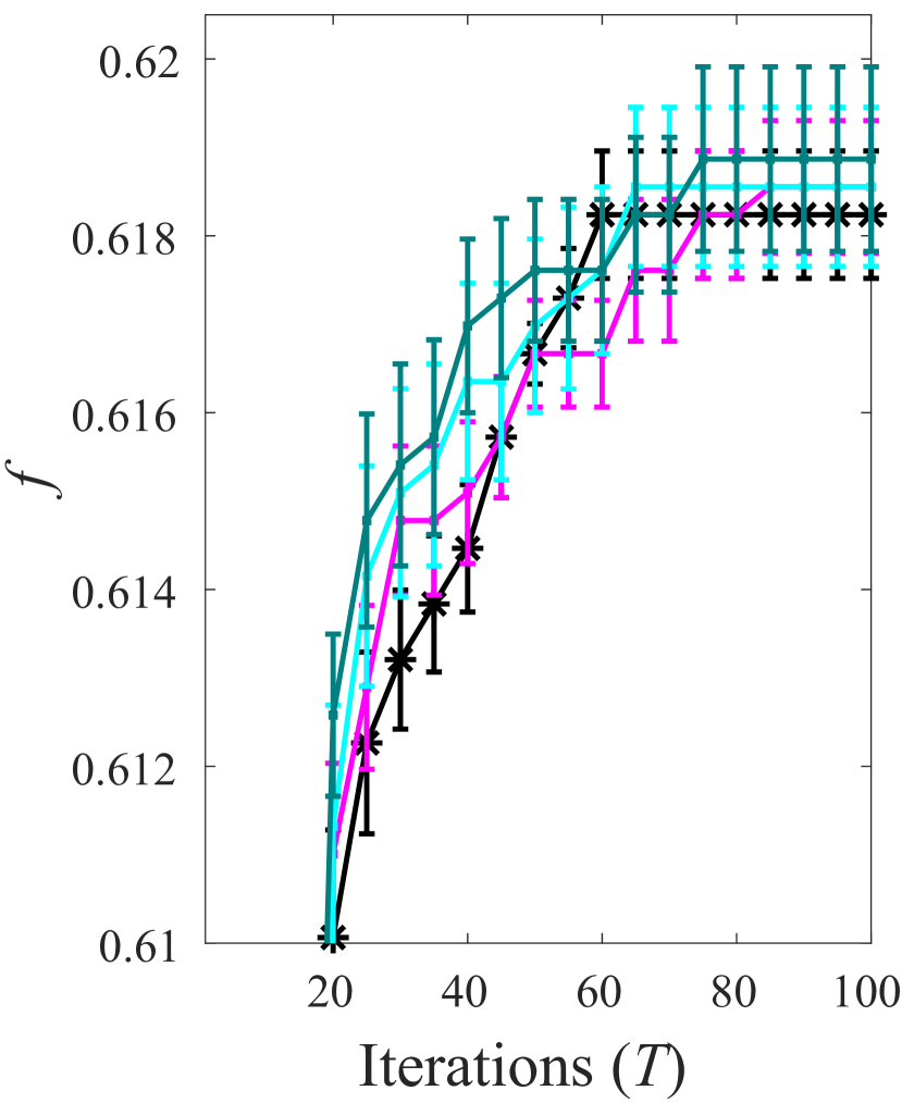
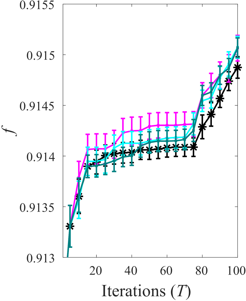
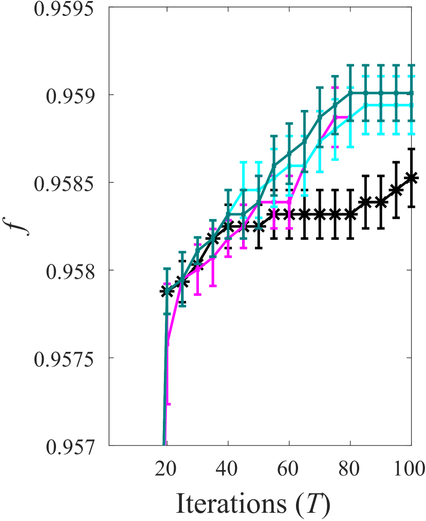
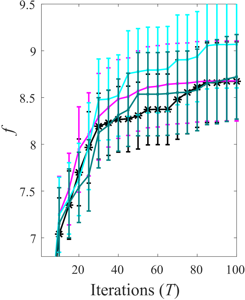
(a) SVM$\_$wine

(b) NN$\_$wine

(c) NN$\_$cancer

(d) NN$\_$housing

Figure 1. The results (mean$\pm$(1/4)std.) of UCB-PP and UCB on real-world optimization problems. $f$: the larger, the better.

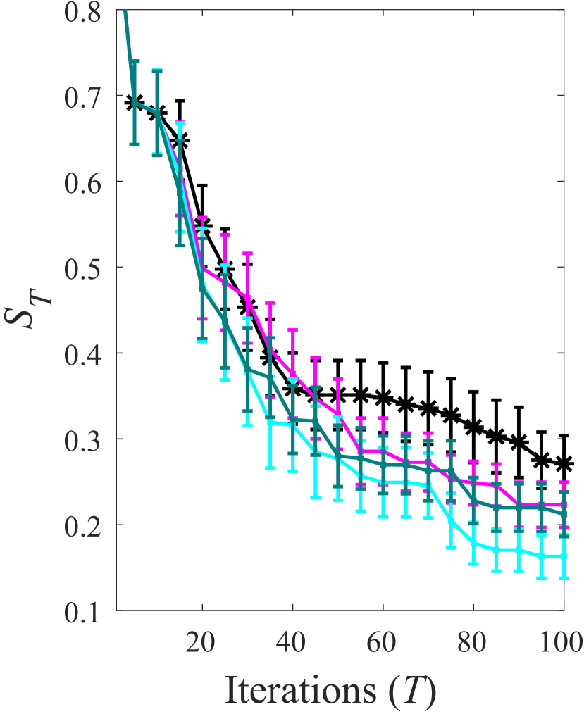
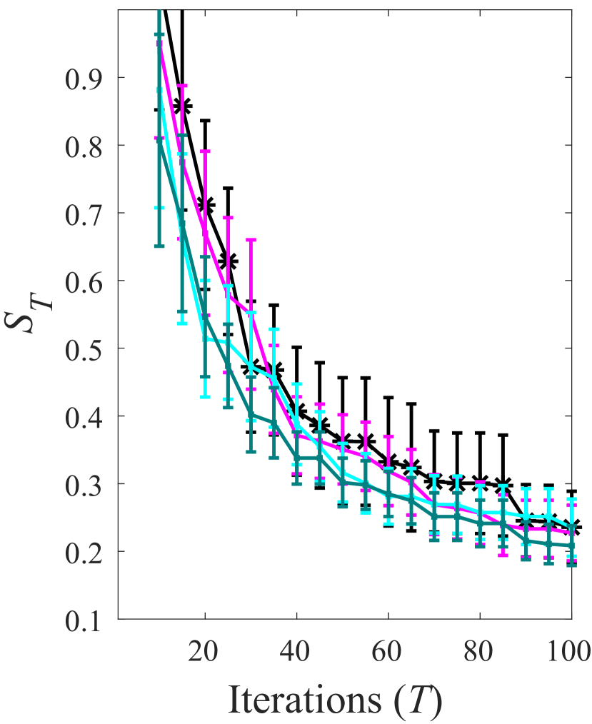
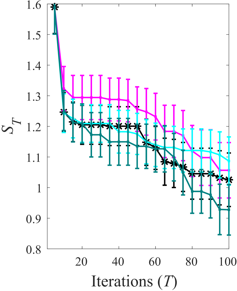
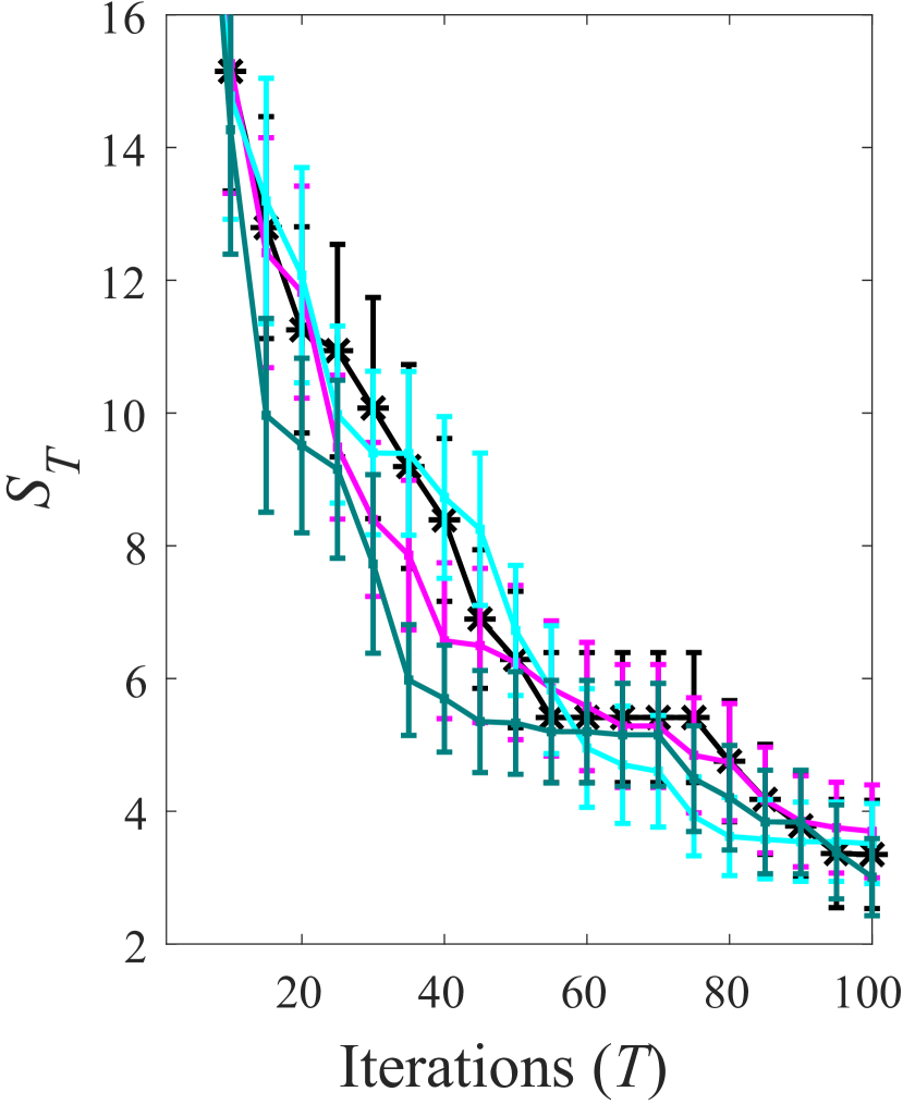
(a) Dropwave

(b) Griewank

(c) Hart6

(d) Rastrigin

Figure 2. The results (mean$\pm$(1/4)std.) of UCB-PP and UCB on synthetic benchmark functions. $S_{T}$: the smaller, the better.

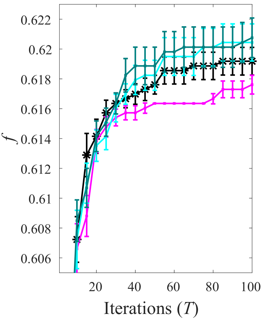
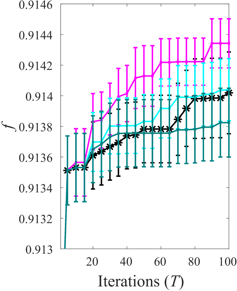
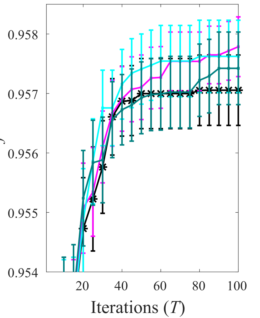
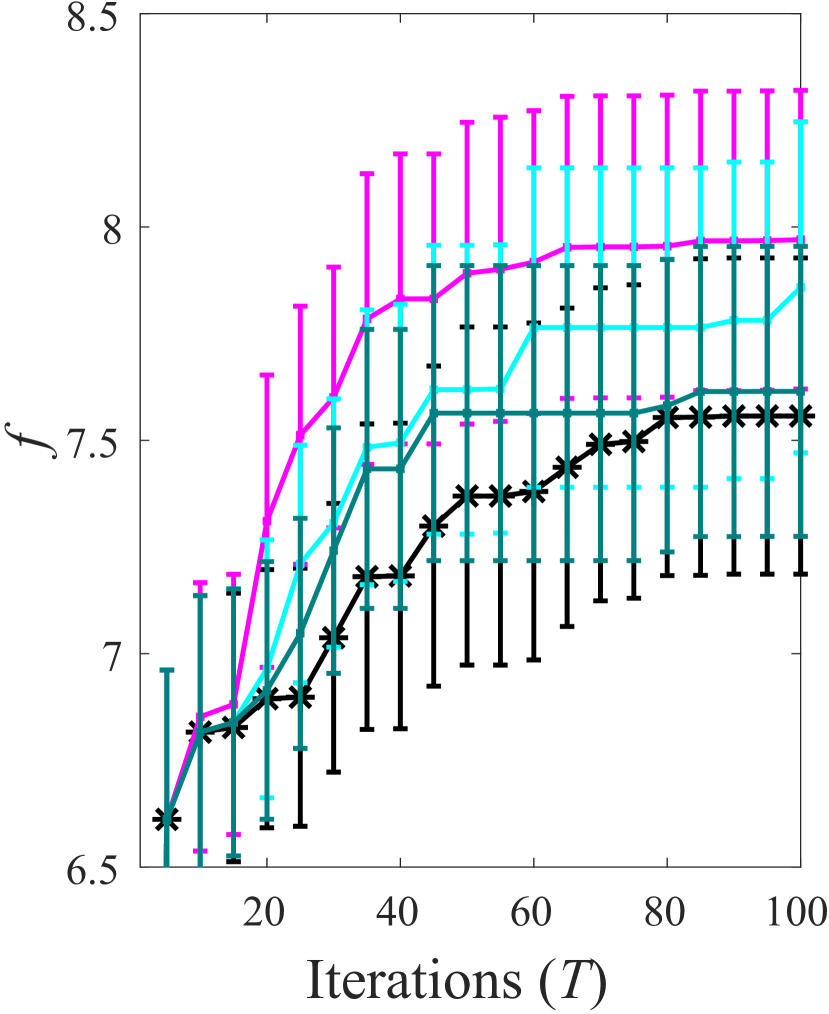
(a) SVM$\_$wine

(b) NN$\_$wine

(d) NN$\_$cancer

(c) NN$\_$housing

Figure 3. The results (mean$\pm$(1/4)std.) of PI-PP and PI on real-world optimization problems. $f$: the larger, the better.

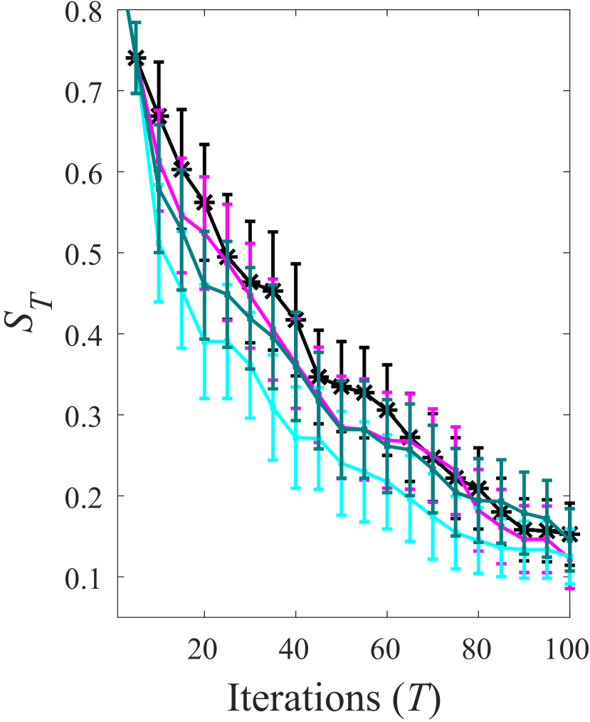
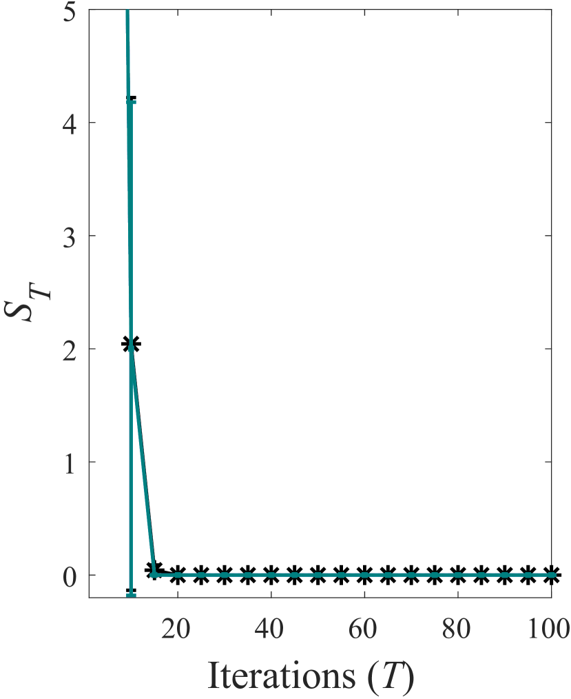
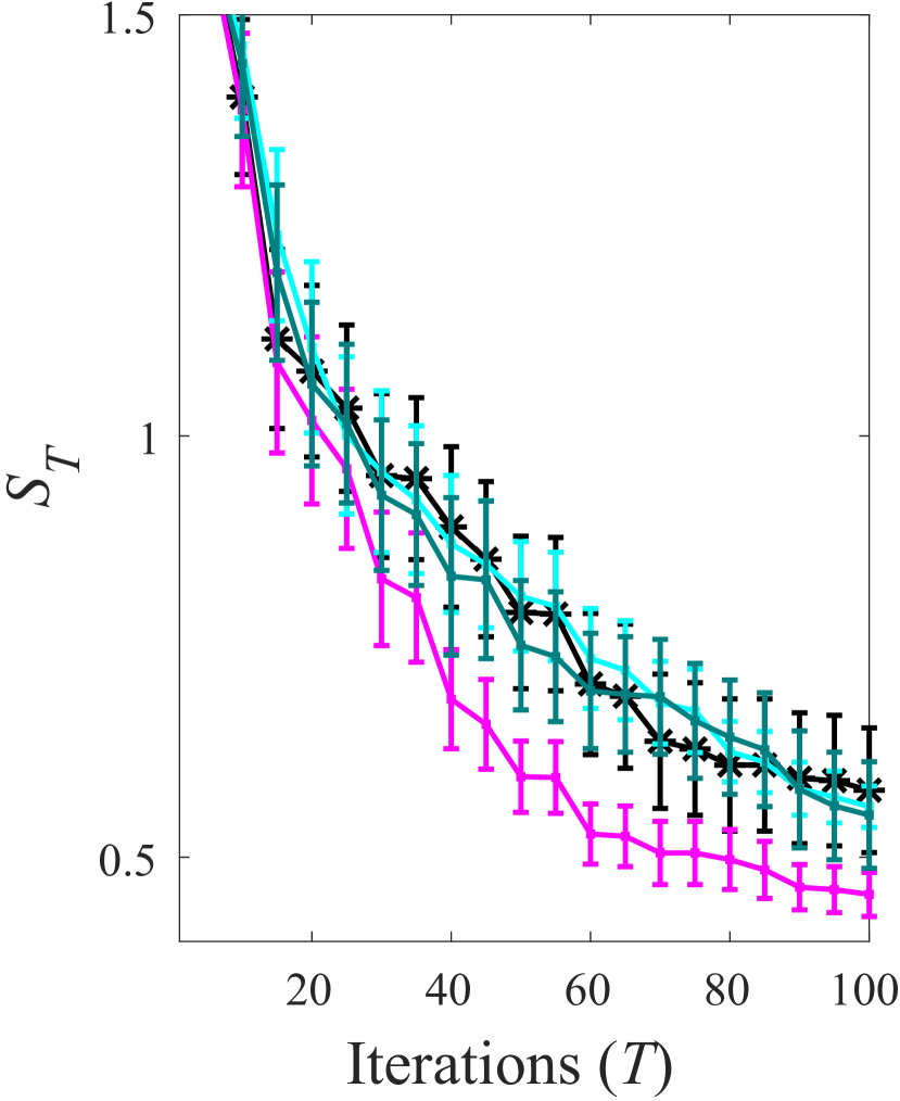
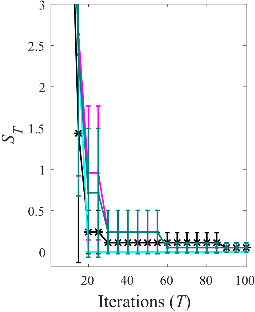
(a) Dropwave

(b) Griewank

(c) Hart6

(d) Rastrigin

Figure 4. The results (mean$\pm$(1/4)std.) of PI-PP and PI on synthetic benchmark functions. $S_{T}$: the smaller, the better.

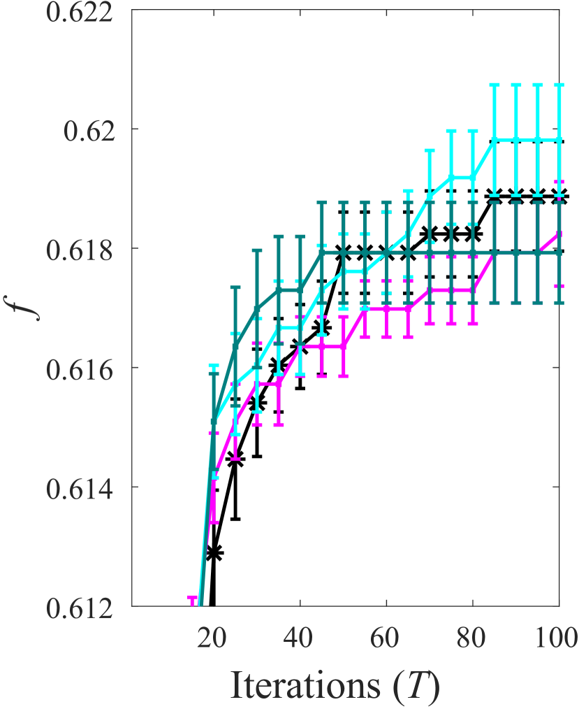
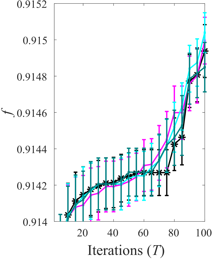
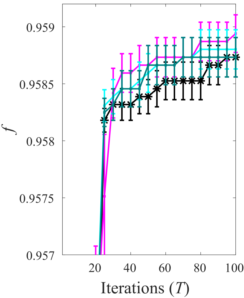
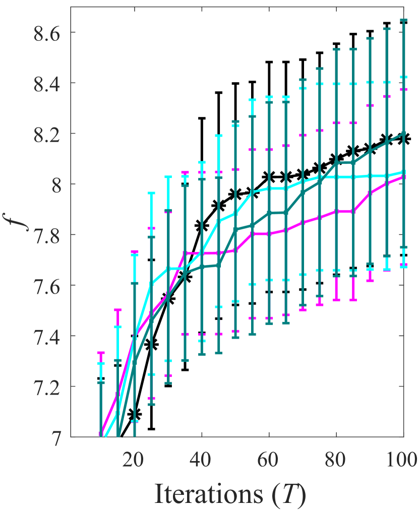
(a) SVM$\_$wine

(b) NN$\_$wine

(c) NN$\_$cancer

(d) NN$\_$housing

Figure 5. The results (mean$\pm$(1/4)std.) of EI-PP and EI on real-world optimization problems. $f$: the larger, the better.

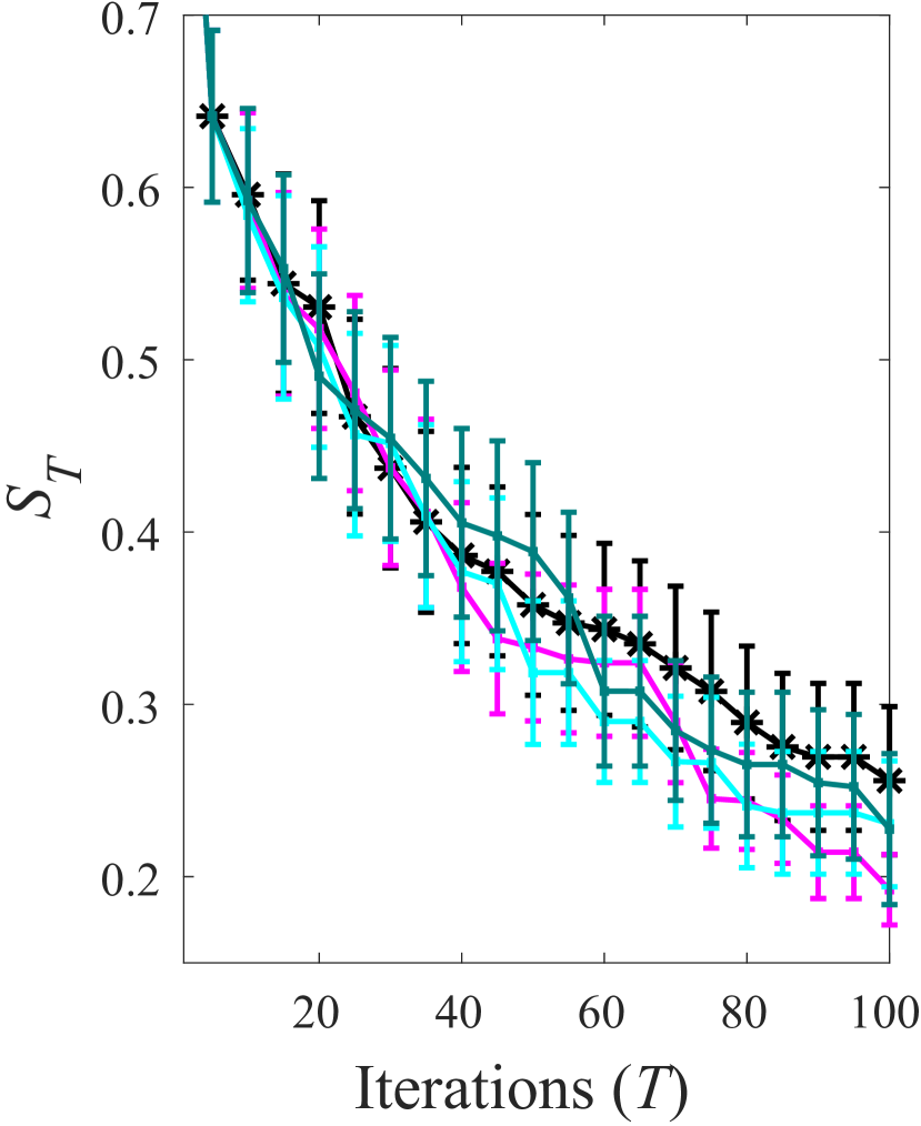
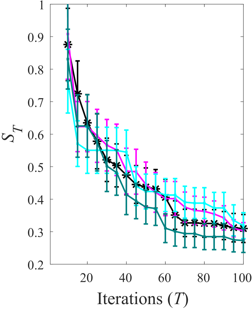
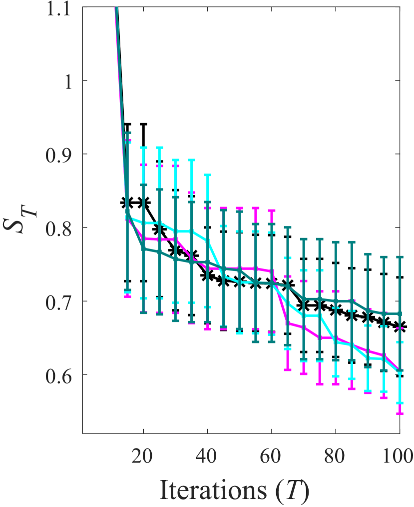
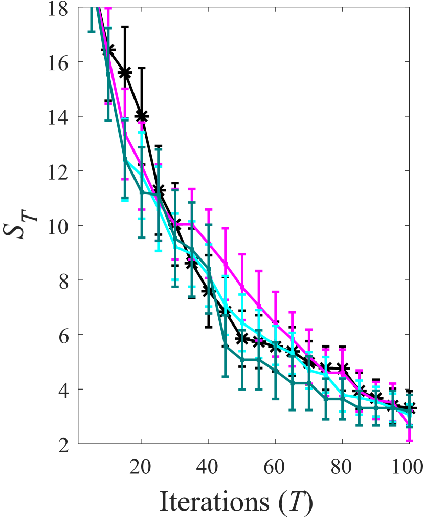
(a) Dropwave

(b) Griewank

(c) Hart6

(d) Rastrigin

Figure 6. The results (mean$\pm$(1/4)std.) of EI-PP and EI on synthetic benchmark functions. $S_{T}$: the smaller, the better.

To examine the robustness of BO-PP against kernels, we use the Gaussian kernel with hyper-parameters tuned by MLE. We compare UCB-PP with UCB on real-world problems, and the results in Figure 7 show that UCB-PP can always be better except UCB-PP01 and UCB-PP001 on SVM$\_$wine.

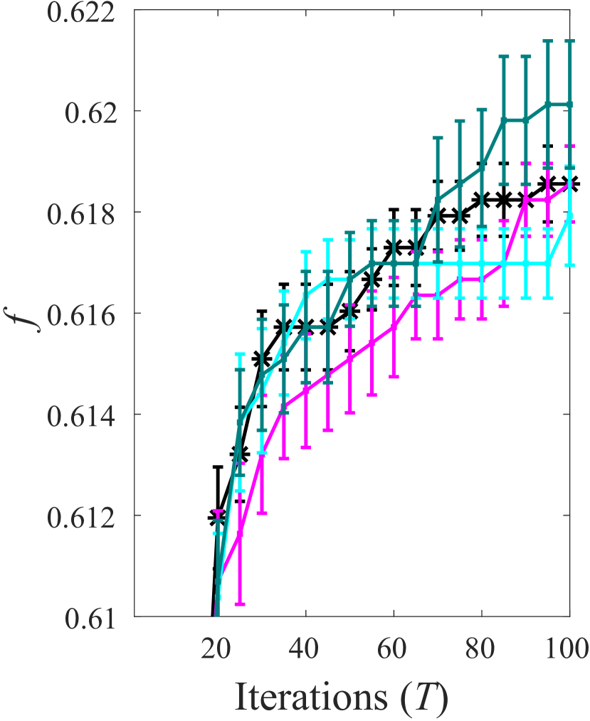
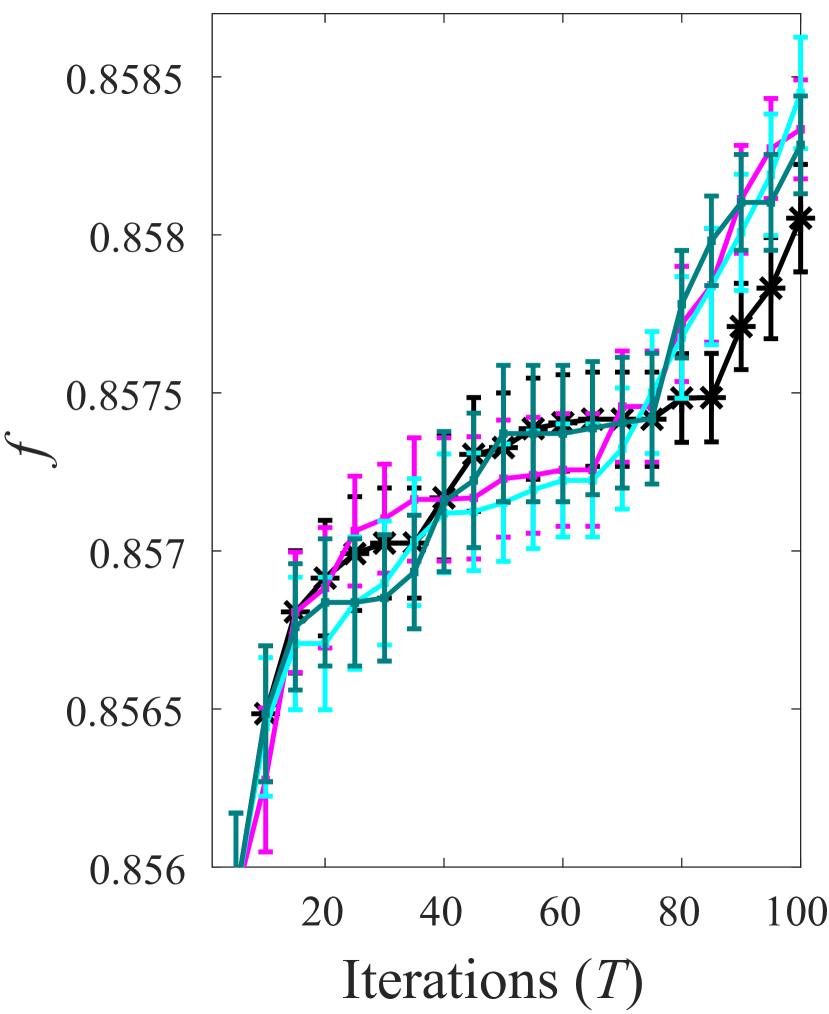
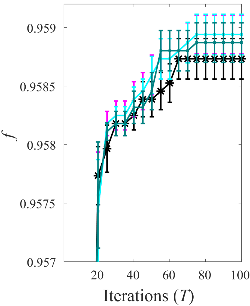
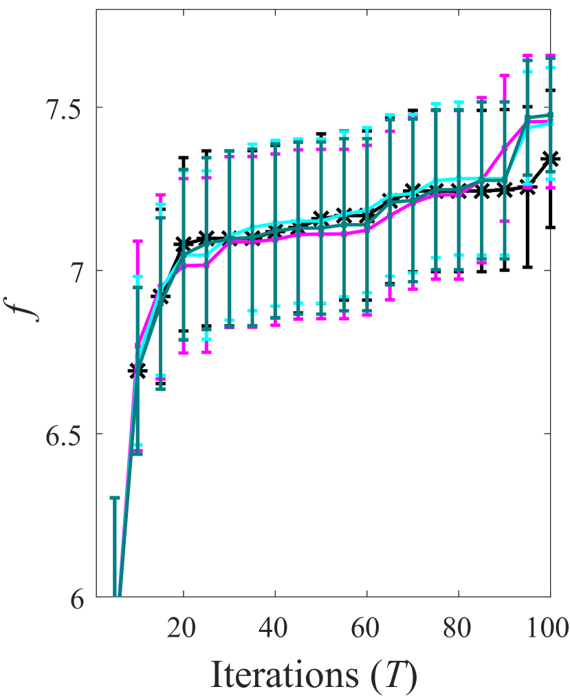
(a) SVM$\_$wine

(b) NN$\_$wine

(c) NN$\_$cancer

(d) NN$\_$housing

Figure 7. The results (mean$\pm$(1/4)std.) of UCB-PP and UCB with the Gaussian kernel on real-world optimization problems. $f$: the larger, the better.

6. Conclusion

In this paper, we propose a general framework BO-PP by generating pseudo-points to improve the GP model of BO. BO-PP can be implemented with any acquisition function. Equipped with UCB, we prove that the cumulative regret of BO-PP can be well bounded. Experiments with UCB, PI and EI on synthetic as well as real-world optimization problems show the excellent performance of BO-PP. It is expected that the generation of pseudo-points can be helpful for more BO algorithms.

References

- (1)
- Azimi et al. (2010) J. Azimi, A. Fern, and X. Z. Fern. 2010. Batch Bayesian optimization via simulation matching. In Advances in Neural Information Processing Systems 23 (NIPS’10). Vancouver, Canada, 109–117.
- Brochu et al. (2010) E. Brochu, V. M. Cora, and N. de Freitas. 2010. A tutorial on Bayesian optimization of expensive cost functions, with application to active user modeling and hierarchical reinforcement learning. CoRR abs/1012.2599 (2010).
- Denil et al. (2012) M. Denil, L. Bazzani, H. Larochelle, and N. de Freitas. 2012. Learning where to attend with deep architectures for image tracking. Neural Computation 24, 8 (2012), 2151–2184.
- Desautels et al. (2014) T. Desautels, A. Krause, and J. W. Burdick. 2014. Parallelizing exploration-exploitation tradeoffs in Gaussian process bandit optimization. Journal of Machine Learning Research 15 (2014), 3873–3923.
- Garnett et al. (2010) R. Garnett, M. A. Osborne, and S. J. Roberts. 2010. Bayesian optimization for sensor set selection. In Proceedings of the 9th ACM/IEEE International Conference on Information Processing in Sensor Networks (IPSN’10). Stockholm, Sweden, 209–219.
- González et al. (2016) J. González, Z. Dai, P. Hennig, and N. D. Lawrence. 2016. Batch Bayesian optimization via local penalization. In Proceedings of the 19th International Conference on Artificial Intelligence and Statistics (AISTATS’16). Cadiz, Spain, 648–657.
- Hennig and Schuler (2012) P. Hennig and C. J. Schuler. 2012. Entropy search for information-efficient global optimization. Journal of Machine Learning Research 13 (2012), 1809–1837.
- Hernández-Lobato et al. (2014) J. M. Hernández-Lobato, M. W. Hoffman, and Z. Ghahramani. 2014. Predictive entropy search for efficient global optimization of black-box functions. In Advances in Neural Information Processing Systems 27 (NIPS’14). Montreal, Canada, 918–926.
- Jones et al. (1993) D. R. Jones, C. D. Perttunen, and B. E. Stuckman. 1993. Lipschitzian optimization without the Lipschitz constant. Journal of Optimization Theory and Applications 79, 1 (1993), 157–181.
- Jones et al. (1998) D. R. Jones, M. Schonlau, and W. J. Welch. 1998. Efficient global optimization of expensive black-box functions. Journal of Global Optimization 13, 4 (1998), 455–492.
- Kandasamy et al. (2015) K. Kandasamy, J. G. Schneider, and B. Póczos. 2015. High dimensional Bayesian optimisation and bandits via additive models. In Proceedings of the 32nd International Conference on Machine Learning (ICML’15). Lille, France, 295–304.
- Kushner (1964) H. J. Kushner. 1964. A new method of locating the maximum point of an arbitrary multipeak curve in the presence of noise. Journal of Basic Engineering 86, 1 (1964), 97–106.
- Lyu et al. (2018) W. Lyu, F. Yang, C. Yan, D. Zhou, and X. Zeng. 2018. Batch Bayesian optimization via multi-objective acquisition ensemble for automated analog circuit design. In Proceedings of the 35th International Conference on Machine Learning (ICML’18). Stockholm, Sweden, 3306–3314.
- Martinez-Cantin et al. (2007) R. Martinez-Cantin, N. de Freitas, A. Doucet, and J. A. Castellanos. 2007. Active policy learning for robot planning and exploration under uncertainty. In Robotics: Science and Systems III (RSS’07). Atlanta, GA, 321–328.
- Mockus (1994) J. Mockus. 1994. Application of Bayesian approach to numerical methods of global and stochastic optimization. Journal of Global Optimization 4, 4 (1994), 347–365.
- Mutny and Krause (2018) M. Mutny and A. Krause. 2018. Efficient high dimensional Bayesian optimization with additivity and quadrature Fourier features. In Advances in Neural Information Processing Systems 31 (NeurIPS’18). Montreal, Canada, 9005–9016.
- Rasmussen and Williams (2006) C. E. Rasmussen and C. Williams. 2006. Gaussian Processes for Machine Learning. The MIT Press, Cambridge, MA.
- Ru et al. (2018) B. X. Ru, M. McLeod, D. Granziol, and M. A. Osborne. 2018. Fast information-theoretic Bayesian optimisation. In Proceedings of the 35th International Conference on Machine Learning (ICML’18). Stockholm, Sweden, 4381–4389.
- Shah and Ghahramani (2015) A. Shah and Z. Ghahramani. 2015. Parallel predictive entropy search for batch global optimization of expensive objective functions. In Advances in Neural Information Processing Systems 28 (NIPS’15). Montreal, Canada, 3330–3338.
- Snoek et al. (2012) J. Snoek, H. Larochelle, and R. P. Adams. 2012. Practical Bayesian optimization of machine learning algorithms. In Advances in Neural Information Processing Systems 25 (NIPS’12). Lake Tahoe, NV, 2951–2959.
- Springenberg et al. (2016) J. T. Springenberg, A. Klein, S. Falkner, and F. Hutter. 2016. Bayesian optimization with robust Bayesian neural networks. In Advances in Neural Information Processing Systems 29 (NIPS’16). Barcelona, Spain, 4134–4142.
- Srinivas et al. (2012) N. Srinivas, A. Krause, S. M. Kakade, and M. W. Seeger. 2012. Information-theoretic regret bounds for Gaussian process optimization in the bandit setting. IEEE Transactions on Information Theory 58, 5 (2012), 3250–3265.
- Wang and Jegelka (2017) Z. Wang and S. Jegelka. 2017. Max-value entropy search for efficient Bayesian optimization. In Proceedings of the 34th International Conference on Machine Learning (ICML’17). Sydney, Australia, 3627–3635.
- Wang et al. (2017) Z. Wang, C. Li, S. Jegelka, and P. Kohli. 2017. Batched high-dimensional Bayesian optimization via structural kernel learning. In Proceedings of the 34th International Conference on Machine Learning (ICML’17). Sydney, Australia, 3656–3664.
- Wang et al. (2016) Z. Wang, B. Zhou, and S. Jegelka. 2016. Optimization as estimation with Gaussian processes in bandit settings. In Proceedings of the 19th International Conference on Artificial Intelligence and Statistics (AISTATS’16). Cadiz, Spain, 1022–1031.
- Wang et al. (2013) Z. Wang, M. Zoghi, F. Hutter, D. Matheson, and N. de Freitas. 2013. Bayesian optimization in high dimensions via random embeddings. In Proceedings of the 23rd International Joint Conference on Artificial Intelligence (IJCAI’13). Beijing, China, 1778–1784.