Analytical Performance Evaluation of Beamforming Under Transceivers Hardware Imperfections

Abstract

In this paper, we provide the mathematical framework to evaluate and quantify the performance of wireless systems, which employ beamforming, in the presence of hardware imperfections at both the basestation and the user equipment. In more detail, by taking a macroscopic view of the joint impact of hardware imperfections, we introduce a general model that accounts for transceiver impairments in beamforming transmissions. In order to evaluate their impact, we present novel closed form expressions for the outage probability and upper bounds for the characterization of the system’s capacity. Our analysis reveals that the level of imperfection can significantly constraint the ergodic capacity. Therefore, it is important to take them into account when evaluating and designing beamforming systems.

I Introduction

The increased data rates demand, in the beyond fifth generation (5G) wireless systems, as well as the fact that the spectral efficiency of the microwave links is approaching its fundamental limits have motivated the exploitation of higher frequency bands that offer abundance of communication bandwidth [1, 2, 3]. Towards this end, higher unlicensed bands, such as millimeter wave (mmW) and terahertz (THz), for wireless communications have been recognized as attractive canditates [4, 5].

Although these communication bands can benefit from an extreme increase in the bandwidth, it comes at the price of suffering severe path loss, which drastically limits the links range [6, 7]. To overcome this problem, a great amount of research effort has been put on investigating the use of multiple antennas in order to achieve link-level directional beamforming [8, 9, 10]. However, most of the published papers in the context of mmW and THz wireless systems make the standard assumption of ideal transceiver hardware.

In practice, hardware suffers from several types of impairments, such as phase noise, in-phase (I) and quadrature (Q) imbalance, and amplifier nonlinearities (see [11] and reference therein). The impact of hardware impairments on various types of communication systems was analyzed in [12, 13, 14, 15, 16]. In particular, in [12], the authors investigated the impact of phase noise in multiple-input multiple-ouput (MIMO) orthogonal frequency division multiplexing (OFDM) systems, whereas, in [13], the authors analyzed the performance of MIMO system in the presence of I/Q imbalance. Moreover, in [14], the impact of I/Q imbalance in amplify and forward (AF) relaying systems was quantified. Finally, a generalized model that takes into account the joint impact of I/Q imbalance, phase noise and non-linearities was presented in [15], while, in [16], the authors used this model to evaluate the impact of hardware imperfections in dual hop AF relaying systems. As a general conclusion, hardware impairments have a deleterious impact on the achievable performance, especially in high data rate systems [11, 17, 18, 19, 20].

In spite of the paramount importance of hardware impairments on wireless systems, their detrimental effect has been overlooked in the analysis of wireless systems that employ beamforming. Motivated by this, the present work is devoted to the quantification of the impact of hardware impairments on the performance of beamforming transmissions. In more detail, the technical contribution of the paper is outlined below:

• We introduce a general model to account for transceiver impairments in beamforming transmissions. Unlike [21, 22], which study the effect of a single type imperfection, in this work, we take a macroscopic view and examine the joint impact of hardware impairments.

• After deriving the instantaneous signal-to-noise-plus-distortion-ratio (SNDR), we present a novel closed-form expressions for the exact outage probability of the system. This expression enables the quantification of the impact of hardware imperfection of the performance of the systems. Additionally, they can be used to select the transmission data rate and the number of antennas that are required to satisfy an outage probability specification. Moreover, we present simple closed-form expressions for the outage probability that corresponds to the special case in which all radio frequency (RF) chains suffer from the same level of imperfections.

• Moreover, in order to characterize the ergodic capacity of the beamforming channel, we derive a simple close-form expression for its upper bound.

• Finally, we provide simple expressions for the capacity ceilings, when the signal-to-noise ratio (SNR) and or the number of transmit antennas tend to infinity.

The remainder of the paper is organized as follows: Section II presents the system model, while Section III is devoted to the derivation of the analytic expression for the outage probability. Respective numerical results and discussions are provided in Section IV, whereas closing remarks are presented in Section V.

Notations: Unless otherwise stated, lower and upper case bold letters denote vectors and matrices, respectively. The matrix $\mathbf{0}_{N\times M}$ stand for the all zero $N\times M$ matrix. The operator $\mathrm{diag}\left(\mathbf{x}\right)$ returns a matrix with the elements of the vector $\mathbf{x}$ on the leading diagonal, and $0$ elsewhere. Also, $(\cdot)^{*}$ and $(\cdot)^{t}$ denote the matrix complex-conjugate and transpose operations, respectively. The operator $||\mathbf{x}||$ represents the norm of the vector $\mathbf{x}$, while $|x|$ is the absolute time of the variable $x$. $\mathbb{E}[\mathcal{X}]$ stands for the expected value of the random variable $\mathcal{X}$, while $\exp(x)$ and $\log_{2}(x)$ return the exponential and the the base-2 logarithm of $x$, respectively. Finally, the lower incomplete Gamma functionis represented as $\gamma\left(\cdot,\cdot\right)$ [23, Eq. (8.350/1)], while the Gamma function is denoted by $\Gamma\left(\cdot\right)$ [23, Eq. (8.310)].

II System and Signal Model

\psfrag{A}[1]{$1$}\psfrag{B}[1]{$2$}\psfrag{C}[1]{$N_{t}$}\psfrag{D}[1]{BS}\psfrag{E}[1]{UE}\includegraphics[width=260.17464pt,trim=0.0pt 0.0pt 0.0pt 0.0pt,clip={false}]{sm.eps}

Figure 1: System model.

As presented in Fig. 1, we consider a downlink scenario of a classical wireless system, in which the basestation (BS) is equipped with $N_{t}$ antennas, while the user equipment (UE) has a single antenna. The BS is assumed to perform digital beamforming, i.e., each antenna is driven by an individual RF chain. Moreover, we assume perfect channel state information (CSI) at the BS.

At the BS, the information symbol, $s$, is pre-coded using the $N_{t}\times 1$ beamforming vector, $\mathbf{p}$. We set $||\mathbf{p}||=1$, to reflect the power constraint at the BS. Note that the maximum signal to noise ratio (SNR) is achieved, if $\mathbf{p}$ is proportional to $\mathbf{h}^{*}$, i.e.,

$$\mathbf{p}=\frac{\mathbf{h}^{*}}{||\mathbf{h}^{*}||},$$ (1)

where $\mathbf{h}$ stand for the baseband equivalent channel.

The transmitted signal, $\mathbf{x}=\mathbf{p}s$, is conveyed over the flat fading wireless channel, $\mathbf{h}$, with additive noise $n\in\mathbb{C}$. Note that this channel can, for instance, be one of the subcarriers in a multi-carrier system. By assuming ideal radio frequency (RF) front end at both the BS and UE, the received signal can be modeled as

$$y=\mathbf{h}^{t}\mathbf{x}+n,$$ (2)

where $\mathbf{h}^{t}$ and ${n}$ are statistically independent. Note that due to the relatively small bandwidth of the subcarrier, $n$ can be approximated as a zero mean complex Gaussian process with single-sided power spectrum densities (PSD) of $N_{0}$ [26]. Moreover, the channel vector

$$\mathbf{h}= \left[|h_{1}|\exp(-j2\pi\phi_{1}),|h_{2}|\exp(-j2\pi\phi_{2}),\cdots,\right.$$

$$\hskip 99.58464pt\left.|h_{N_{t}}|\exp(-j2\pi\phi_{N_{t}})\right]^{t},$$ (3)

where $|h_{i}|$ and $\phi_{i}$, $i\in[1,N_{t}]$, denote the amplitude and phase of the channel of the $i-$th BS antenna and the UE. Finally, it is assumed that $|h_{i}|$ follows Rayleigh.

The conventional received signal model, described by (2), cannot capture the impact of hardware imperfections. Due to these imperfections, each RF chain, $i$ with $i\in[1,N_{t}]$, at the BS causes a mismatch between the intended transmitted signal, $x_{i}$, and what is actually generated and emitted. As a consequence, the actual transmitted signal can be modeled as

$$\tilde{\mathbf{x}}=\mathbf{x}+\mathbf{W}_{b}\mathbf{p},$$ (4)

where $\mathbf{W}_{b}=\mathrm{diag}\left([w_{b,1},w_{b,2},\cdots,w_{b,N}]\right)$ represent the distortion noise from impairments at the BS. Similarly, at the UE, the baseband equivalent received signal can be expressed as

$$\tilde{y}=\mathbf{h}^{t}\left(\mathbf{x}+\mathbf{W}_{b}\mathbf{p}\right)+w_{u}+n,$$ (5)

where $w_{u}$ stands for the distortion noise from the impairments at the UE. The distortion noises are defined as [11, 16, 17]

$$\mathbf{w}_{b} \sim\mathcal{CN}\left(\mathbf{0}_{N_{t}\times N_{t}},\mathrm{diag}\left(\left[k_{b,1}^{2},k_{b,2}^{2},\cdots,k_{b,N}^{2}\right]\right)P_{s}\right),$$ (6)

$$w_{u} \sim\mathcal{CN}\left(0,k_{u}^{2}P_{s}||\mathbf{h}||^{2}\right),$$ (7)

where $k_{b,i}$ ($i=1,2,\cdots,N$) and $k_{u}$ are non-negative design parameters that characterize the level of imperfection in the BS and UE hardware, respectively, whereas $P_{s}$ stands for the average received signal power. This model has been validated by several theoretical and experimental results, see e.g., [29, 30, 31] and references therein. Note that for $k_{b,1}=k_{b,2}=\cdots=k_{b,N}=k_{u}=0$, i.e., in the case of ideal RF chains at both the BS and UE, (5) is simplified into (2).

III Performance Analysis

In this section, after we derive the SNDR, we evaluate the system’s outage probability and we characterize the ergodic capacity.

III-A SNDR

Based on (5)-(7) and after some basic algebraic manipulations, the SNDR can be expressed as

$$\gamma=\frac{||\mathbf{h}||^{2}P_{s}}{\sum_{i=1}^{N}(k_{b,i}^{2}+k_{u}^{2})|h_{0i}|^{2}P_{s}+N_{0}}.$$ (8)

From (8), it is evident that as the number of antennas increases the diversity gain increases together with the level of interference, due to the hardware imperfections. Moreover, a transmission power increase leads to a linear increase of the interference level. Finally, we observe that as the level of imperfection increases, i.e., as $k_{b,i}^{2}+k_{u}^{2}$, $i=1,2,\cdots,N_{t}$, the SNDR decreases. Note that according to the third generation partnership project (3GPP) long term evolution advanced (LTE-A), the parameters $k_{b,i}$ and $k_{u}$ are in the range of $[0.08,0.175]$ [32].

III-B Outage probability

In order to quantify the impact of hardware imperfections on the system’s performance, as well as to provide design criteria for wireless systems that employ digital beamforming schemes, we derive the outage probability. The following proposition returns the outage probability.

Proposition 1

The outage probability can be obtained as

$$P_{o}(r_{\mathrm{th}})=\sum_{i=1}^{N_{t}}\Xi(i,1,b_{i})\left(1-\exp\left({-\frac{2^{r_{\mathrm{th}}}-1}{\tilde{\gamma}b_{i}}}\right)\right),$$ (9)

where $r_{\mathrm{th}}$ is the minimum allowable (threshold) rate, $\Xi(i,1,b_{i})$ is defined in [33, Eqs. (8) and (9)],

$$b_{i}=1-\left(k_{b,i}^{2}+k_{u}^{2}\right)\left(2^{r_{\mathrm{th}}}-1\right),$$ (10)

and

$$\tilde{\gamma}=\frac{P_{s}}{N_{0}}.$$ (11)

Proof:

Please refer to the Appendix A. ∎

Note that $\Xi\left(\cdot,1,b_{i}\right)$ depends on the level of hardware imperfections and $r_{\mathrm{th}}$. In other words, in contrast with the ideal RF chains scenario, the outage probability does not only depends on the SNR and the $r_{\mathrm{th}}$, but also on the values of $k_{b,i}$, $i=1,2,\cdots,N_{t}$ and $k_{u}$.

The following remark presents a design criterion that should be taken into consideration when designing a digital beamforming scheme.

Remark 1

From (25), it is observed that a link between the $i-$th antenna of the BS and the UE, in which $\left(k_{b,i}^{2}+k_{u}^{2}\right)\left(2^{r_{\mathrm{th}}}-1\right)>1$, has a negative impact on the performance of the beamforming scheme.

Special case

In the special case in which $k_{b,1}=k_{b,2}=\cdots=k_{b,N_{t}}=k_{b}$, $b_{1}=b_{2}=\cdots=b_{N_{t}}=b$ and the random variable $\mathcal{X}$, defined in Appendix B (25), follows chi-square distribution, which CDF given by

$$F_{\mathcal{X}}^{\mathrm{sc}}(x)=\frac{\gamma\left(N_{t},\frac{x}{b}\right)}{\Gamma{(N_{t})}},$$ (12)

which, by taking into account that $N_{t}$ is an integer, can be simplified as

$$F_{\mathcal{X}}^{\mathrm{sc}}(x)=1-\sum_{k=0}^{N_{t}-1}\frac{x^{k}}{b^{k}k!}\exp\left(-\frac{x}{b}\right).$$ (13)

Hence, in this case, the outage probability can be evaluated as

$$P_{o}^{\mathrm{sc}}=F_{\mathcal{X}}^{\mathrm{sc}}\left(\frac{\gamma_{\mathrm{th}}}{\tilde{\gamma}}\right).$$ (14)

or, equivalently

$$P_{o}^{\mathrm{sc}}=1-\sum_{k=0}^{N_{t}-1}\frac{\gamma_{\mathrm{th}}^{k}}{\tilde{\gamma}^{k}b^{k}k!}\exp\left(-\frac{\gamma_{\mathrm{th}}}{\tilde{\gamma}b}\right)$$ (15)

III-C Ergodic capacity

To characterize the ergodic capacity of the beamforming channel, an upper bound is derived by the following proposition.

Proposition 2

The ergodic capacity, $C$, (in bits/channel use) with beamforming and non-ideal hardware is upper bounded as

$$C\leq\log_{2}\left(1+\frac{N_{t}}{\sum_{i=1}^{N_{t}}{\Xi(i,1,c_{i})}{c_{i}}+\frac{1}{\tilde{\gamma}}}\right),$$ (16)

where $c_{i}$ can be obtained as

$$c_{i}=k_{b,i}^{2}+k_{u}^{2},$$ (17)

with $i\in[1,N_{t}]$.

Proof:

Please refer to the Appendix B. ∎

Corollary 1 (Capacity ceiling)

As the SNR tends to infinity, the ergodic capacity is constraint by

$$\lim_{\tilde{\gamma}\to\infty}C=\log_{2}\left(1+\frac{N_{t}}{\sum_{i=1}^{N_{t}}{\Xi(i,1,c_{i})}{c_{i}}}\right).$$ (18)

Proof:

Based on (16), the capacity ceiling can be expressed as

$$\lim_{\tilde{\gamma}\to\infty}C \leq\lim_{\tilde{\gamma}\to\infty}\left(\log_{2}\left(1+\frac{N_{t}}{\sum_{i=1}^{N_{t}}{\Xi(i,1,c_{i})}{c_{i}}+\frac{1}{\tilde{\gamma}}}\right)\right)$$

$$=\log_{2}\left(1+\frac{N_{t}}{\sum_{i=1}^{N_{t}}{\Xi(i,1,c_{i})}{c_{i}}}\right).$$ (19)

This concludes the proof. ∎

Special case

In the special case in which $k_{b,1}=k_{b,2}=\cdots=k_{b,N_{t}}=k_{b}$, the random variable $\mathcal{Y}$, defined in (35), follows chi-square distribution, with $N_{t}$ degrees of freedom; hence, $\mathbb{E}\left[\mathcal{Y}\right]=N_{t}\left(k_{b}^{2}+k_{u}^{2}\right)$, and the ergodic capacity is upper bounded as

$$C^{\mathrm{sc}}\leq\log_{2}\left(1+\frac{N_{t}}{N_{t}\left(k_{b}^{2}+k_{u}^{2}\right)+\frac{1}{\tilde{\gamma}}}\right).$$ (20)

From (20), it is evident that in the high SNR regime, the ergodic capacity satisfies

$$\lim_{\tilde{\gamma}\to\infty}C^{\mathrm{sc}}=\log_{2}\left(1+\frac{1}{k_{b}^{2}+k_{u}^{2}}\right).$$ (21)

Moreover, for a given $\tilde{\gamma}$, as the number of antennas increases, the capacity tends to

$$\lim_{N_{t}\to\infty}C^{\mathrm{sc}}=\log_{2}\left(1+\frac{1}{k_{b}^{2}+k_{u}^{2}}\right).$$ (22)

From (21), we observe that in the high SNR regime, the performance of the system is independent from the number of antennas at the BS and are fully determined by the level of imperfections. Finally, (22) indicates the detrimental effect of hardware imperfection in massive MIMO systems that employ digital beamforming.

IV Results & Discussion

In this section, we validate the theoretical analysis with Monte-Carlo simulations. Furthermore, it is important to note that, unless otherwise is stated, in the following figures, the numerical results are shown with continuous lines, while markers are employed to illustrate the simulation results.

To this end, Fig. 2 illustrates the outage probability versus the SNR for different values of $N_{t}$, assuming that $k_{b,i}=0.16$, $i\in[1,N_{t}]$, $k_{u}=0.1$, and $r_{\mathrm{th}}=2$ (continuous lines). Moreover, in this figure, as a benchmark, we include the corresponding curves when the RF chains at both the BS and UE are considered ideal (dashed lines). As expected, for a given $N_{t}$, as the SNR increases, the outage probability decreases, whereas, for a given SNR, as $N_{t}$ increases, the outage probability decreases. Moreover, the impact of hardware imperfections become more severe as $N_{t}$ increases. For instance, for SNR equals $10$ dB and $N_{t}=2$, the performance loss, due to hardware imperfections is $22.44\%$, whereas for the same SNR and $N_{t}=4$, the performance loss equals $51.94\%$. This indicates the importance of taking into consideration the impact of hardware imperfection, when we select the number of operational RF front-ends.

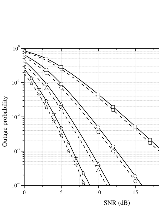
Figure 2: Outage probability as a function of the SNR for different values of $N_{t}$, assuming ideal (dashed lines) and non-ideal (continious lines) RF chains with $k_{b,i}=0.16$, $i\in[1,N_{t}]$, $k_{u}=0.1$, and $r_{\mathrm{th}}=2$.

Fig. 3 depicts the outage probability as a function of SNR, for different values of $r_{\mathrm{th}}$, assuming $N_{t}=2$, $k_{b,1}=0.08$, $k_{b,2}=0.17$, and $k_{u}=0.1$ (continuous lines), as well as the ideal RF chain case (dashed lines). Proposition 1 show perfect agreement with the marker symbols, which are the Monte-Carlo simulation results. For this figure, we observe that, in the low rate threshold, there is only a minor performance loss cause by the hardware imperfections. On the other hand, when the threshold is increased to $r_{\mathrm{th}}=4$ bits/channel use, there is a substantial performance loss. In more detail, for $r_{\mathrm{th}}=2$ and $r_{\mathrm{th}}=4$ bits/channel use, the system experience losses less than $0.5$ dB and about $5$ dB in SNR, respectively. Additionally, we observe that the outage probability curves with non-ideal hardware have the same slop as the ones with the ideal RF chains; therefore, hardware imperfections result in an SNR offset.

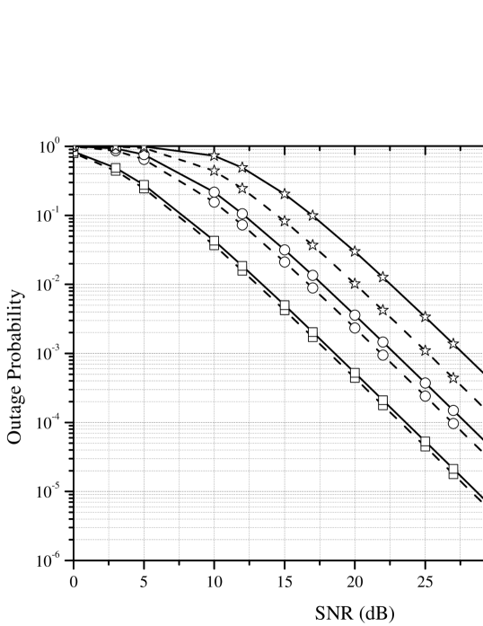
Figure 3: Outage probability as a function of the SNR for different values of $r_{\mathrm{th}}$, assuming ideal (dashed lines) and non-ideal (continious lines) RF chains with $N_{t}=2$, $k_{b,1}=0.08$, $k_{b,2}=0.17$, and $k_{u}=0.1$.

In Fig. 4, the ergodic capacity is plotted as a function of the SNR, for different levels of imperfections. In this figure, the continuous lines represent Monte Carlo simulation results, while the dashed lines stand for the capacity upper bound, which is derived by (16) and (20). Additionally, the dashed-dotted lines denote the capacity ceiling, given by (21). Note that, as a benchmark, the capacity versus SNR for the ideal RF chains case is also plotted. As expected, as SNR increases, the capacity also increases. However, in the case of non-ideal RF chains, the ergodic capacity saturates as approaches the capacity ceiling, as proven from Corollary 1. As a result, since the capacity ceiling is determined by the level of imperfections, it increases as $k_{b,i}$, ($i=1,\cdots,N_{t}$) and $k_{u}$ decreases. Moreover, we observe that the hardware imperfections have a small effect on the ergodic capacity at the low SNR regime, whereas, at the high SNR regime their impact is detrimental. Finally, from this figure, it is evident that the upper bound derived by Proposition 2 and (20), can be used as a simplified capacity approximation. This approximation can be considered tight in the high SNR regime.

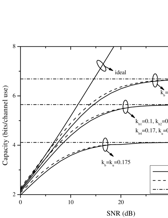
Figure 4: Ergotic capacity as a function of the SNR for different levels of hardware imperfections and $N_{t}=4$.

In Fig. 5, the ergodic capacity is illustrated as a function of the number of antennas for SNR equals $5$ and $10$ dB and $k_{b,i}=k_{u}=0.17$ with $i\in[1,N_{t}]$. Note that the use of a high ammount of $N_{t}$ is a realistic scenario in mmW and THz communications. Moreover, since, in digital beamforming, as the number of antennas increases, the number of corresponding RF chains also increases; hence, the power consumption increases. In this figure, the continuous lines represent Monte Carlo simulation results, the dashed lines stand for the capacity upper bound, which is derived by(20), and the dashed-dotted lines denote the capacity ceiling. From this figure, we observe that in the case of non-ideal RF chains, for a given SNR values, as the number of antennas increases, the ergodic capacity saturates and approaches $\log_{2}\left(1+\frac{1}{k_{b}^{2}+k_{u}^{2}}\right)$. Interestingly, the maximum achievable ergodic capacity is independent of the number of antennas at the BS, but it depends on the level of imperfections at both the BS and UE RF chains. This indicates that the key parameters in order to select the operational number of transmit antennas are the values of $k_{b}$ and $k_{u}$.

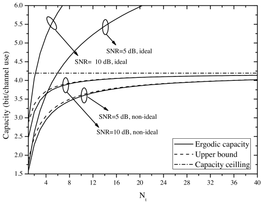
Figure 5: Ergotic capacity as a function of the $N_{t}$ for different levels of SNR and $k_{b,i}=k_{u}=0.17$, $i\in[1,N_{t}]$.

V Conclusions

In this paper, we quantified the impact of hardware imperfections in wireless beamforming systems. In more detail, we provided simple closed form expressions for the system’s outage probability and upper bounds for the ergodic capacity. These expressions take into account the level of imperfections at both the BS and the UE, the transmission and noise power, as well as the number of antennas at the BS. Moreover, through simulation results, we observed that the derived ergodic capacity upper bound can be used as a tight capacity approximation in the high SNR regime. Our results also revealed that there is a capacity ceiling that is independent of the number of transmit antennas, but it is determined by the level of imperfections. Therefore, there is a specific number of transmit antennas after which any further increase will not result to a further significant capacity gain. In other words, it is important for the designer of a digital beamforming system to take into account the level of imperfections in order to select the appropriate number of transmit antennas.

Appendices

Appendix A

Proof of Proposition 1

The outage probability is defined as [34]

$$P_{o}(r_{\mathrm{th}}) =P_{r}\left(\log_{2}\left(1+\gamma\right)\leq r_{\mathrm{th}}\right)=P_{r}\left(\gamma\leq\gamma_{\mathrm{th}}\right),$$ (23)

where $\gamma_{\mathrm{th}}=2^{r_{\mathrm{th}}}-1$.

By substituting (8) into (23), and after some algebraic manipulations, (23) can be equivalently written as

$$P_{o}(r_{\mathrm{th}}) =P_{r}\left(\mathcal{X}\leq\frac{\gamma_{\mathrm{th}}}{\tilde{\gamma}}\right)=F_{\mathcal{X}}\left(\frac{\gamma_{\mathrm{th}}}{\tilde{\gamma}}\right),$$ (24)

where $F_{\mathcal{X}}(\cdot)$ denote the cumulative distribution function (CDF) of $\mathcal{X}$, whereas

$$\mathcal{X}=\sum_{i=1}^{N}\left(1-\left(k_{b,i}^{2}+k_{u}^{2}\right)\gamma_{\mathrm{th}}\right)|h_{0i}|^{2}.$$ (25)

Since $\mathbf{h}$ follows a Saleh-Valenzuela distribution, $|h_{0,i}|$, $i\in[1,N]$, is a Rayleigh distribution random variable. As a consequence, $\mathcal{X}$ is a sum of squared Rayleigh random variable with CDF obtained as [33]

$$F_{\mathcal{X}}(x)=\sum_{i=1}^{N_{t}}\Xi(i,1,b_{i})\left(1-e^{-\frac{x}{b_{i}}}\right).$$ (26)

By setting $x=\frac{\gamma_{\mathrm{th}}}{\tilde{\gamma}}$ into (26), we obtain (9). This concludes the proof.

Appendix B

Proof of Proposition 2

The ergodic capacity is defined as

$$C=\mathbb{E}\left[\log_{2}\left(1+\gamma\right)\right],$$ (27)

or equivalently

$$C=\mathbb{E}\left[\log_{2}\left(1+\frac{\rho}{q}\right)\right],$$ (28)

where, according to (8), $\rho$ and $q$ can be expressed as

$$\rho=\sum_{i=1}^{N_{t}}|h_{0i}|^{2}P_{s}$$ (29)

and

$$q=\sum_{i=1}^{N_{t}}(k_{b,i}^{2}+k_{u}^{2})|h_{0i}|^{2}P_{s}+N_{0}.$$ (30)

By applying Jensen’s inequality [35] into (28), we obtain

$$C\leq\log_{2}\left(1+\frac{\mathcal{A}}{\mathcal{B}}\right),$$ (31)

where $\mathcal{A}=\mathbb{E}\left[\rho\right]$ and $\mathcal{B}=\mathbb{E}\left[q\right]$. Next, we evaluate $\mathcal{A}$ and $\mathcal{B}$.

By taking into consideration (29), $\mathcal{A}$ can be rewritten as

$$\mathcal{A}=P_{s}\mathbb{E}\left[\sum_{i=1}^{N_{t}}|h_{0,i}|^{2}\right].$$ (32)

Since $|h_{0,i}|$ follows Rayleigh distribution $\sum_{i=1}^{N_{t}}|h_{0,i}|^{2}$ is a chi-square distributed random variable with $N_{t}$ degrees of freedom. Therefore, $\mathbb{E}\left[\sum_{i=1}^{N_{t}}|h_{0,i}|^{2}\right]=N_{t}$ and

$$\mathcal{A}=P_{s}N_{t}.$$ (33)

From (25) and (30), $\mathcal{B}$ can be expressed as

$$\mathcal{B}=P_{s}\mathbb{E}[\mathcal{Y}]+N_{0},$$ (34)

where

$$\mathcal{Y}=\sum_{i=1}^{N}\left(k_{b,i}^{2}+k_{u}^{2}\right)|h_{0i}|^{2}.$$ (35)

and the expected value of $\mathcal{X}$ can be evaluated as

$$\mathbb{E}[\mathcal{Y}]=\int_{0}^{\infty}xf_{\mathcal{X}}(x)\mathrm{d}x,$$ (36)

where $f_{\mathcal{Y}}(x)$ is the probability density function of $\mathcal{Y}$. Note that $\mathcal{Y}$, similarly to $\mathcal{X}$, follows sum of square Rayleigh distribution. Therefore, its CDF, $F_{\mathcal{Y}}(x)$ can be obtained by replacing $b_{i}$ with $c_{i}$ into (26), where the probability density function (PDF) can be evaluated as

$$f_{\mathcal{Y}}(x)=\frac{\mathrm{d}F_{\mathcal{Y}}(x)}{\mathrm{d}x}=\sum_{i=1}^{N_{t}}\frac{\Xi(i,1,c_{i})}{c_{i}}e^{-\frac{x}{c_{i}}}.$$ (37)

By substituting (37) into (36), and carrying out the integration, we get

$$\mathbb{E}[\mathcal{Y}]=\sum_{i=1}^{N_{t}}{\Xi(i,1,c_{i})}{c_{i}}.$$ (38)

By substituting (38) into (34), we obtain

$$\mathcal{B}=P_{s}\sum_{i=1}^{N_{t}}{\Xi(i,1,c_{i})}{c_{i}}+N_{0}.$$ (39)

Finally, by substituting (33) and (39) into (31), we get (16). This concludes the proof.

References

- [1] A.-A. A. Boulogeorgos, A. Alexiou, T. Merkle, C. Schubert, R. Elschner, A. Katsiotis, P. Stavrianos, D. Kritharidis, P.-K. Chartsias, J. Kokkoniemi, M. Juntti, J. Lehtomäki, A. Teixeira, and F. Rodrigues, “Terahertz technologies to deliver optical network quality of experience in wireless systems beyond 5G,” IEEE Commun. Mag., Jun. 2018.
- [2] A.-A. A. Boulogeorgos, A. Alexiou, D. Kritharidis, A. Katsiotis, G. Ntouni, J. Kokkoniemi, J. Lethtomaki, M. Juntti, D. Yankova, A. Mokhtar, J.-C. Point, J. Machodo, R. Elschner, C. Schubert, T. Merkle, R. Ferreira, F. Rodrigues, and J. Lima, “Wireless terahertz system architectures for networks beyond 5G,” TERRANOVA CONSORTIUM, White paper 1.0, Jul. 2018.
- [3] A.-A. A. Boulogeorgos and G. K. Karagiannidis, “Low-cost cognitive radios against spectrum scarcity,” IEEE Technical Committee on Cognitive Networks Newsletter, vol. 3, no. 2, pp. 30–34, Nov. 2017.
- [4] R. Piesiewicz, T. Kleine-Ostmann, N. Krumbholz, D. Mittleman, M. Koch, J. Schoebei, and T. Kurner, “Short-range ultra-broadband Terahertz communications: Concepts and perspectives,” IEEE Antennas. Propag., vol. 49, no. 6, pp. 24–39, Dec 2007.
- [5] I. F. Akyildiz, J. M. Jornet, and C. Han, “Terahertz band: Next frontier for wireless communications,” Phys. Commun., vol. 12, pp. 16–32, Sep. 2014.
- [6] A.-A. A. Boulogeorgos, E. N. Papasotiriou, J. Kokkoniemi, J. Lehtomäki, A. Alexiou, and M. Juntti, “Performance evaluation of THz wireless systems operating in 275-400 GHz band,” in IEEE 87th Vehicular Technology Conference: International Workshop on THz Communication Technologies for Systems Beyond 5G, Porto, Portugal, Jun. 2018.
- [7] J. Kokkoniemi, J. Lehtom”aki, and M. Juntti, “Simplified molecular absorption loss model for 275 400 gigahertz frequency band,” in European Conf. Antennas Propag., 2018, pp. 1–5.
- [8] C. Lin and G. Y. Li, “Indoor Terahertz communications: How many antenna arrays are needed?” IEEE Trans. Wireless Commun., vol. 14, no. 6, pp. 3097–3107, Jun. 2015.
- [9] K. Guan, G. Li, T. Kürner, A. F. Molisch, B. Peng, R. He, B. Hui, J. Kim, and Z. Zhong, “On millimeter wave and THz mobile radio channel for smart rail mobility,” IEEE Trans. Veh. Technol., vol. 66, no. 7, pp. 5658–5674, Jul. 2017.
- [10] A.-A. A. Boulogeorgos, E. N. Papasotiriou, and A. Alexiou, “Analytical performance assessment of THz wireless systems,” IEEE Access, vol. 7, no. 1, pp. 1–18, Jan. 2019.
- [11] T. Schenk, RF Imperfections in High-Rate Wireless Systems. The Netherlands: Springer, 2008.
- [12] L. Ju-hu and W. Wei-ling, “Performance of MIMO-OFDM Systems with Phase Noise at Transmit and Receive Antennas,” in 7th Int. Conf. on Wireless Communications, Networking and Mobile Computing, 2011, pp. 1–4.
- [13] J. Qi and S. Aissa, “Analysis and compensation of I/Q imbalance in MIMO transmit-receive diversity systems,” IEEE Trans. Commun., vol. 58, no. 5, pp. 1546–1556, May 2010.
- [14] J. Li, M. Matthaiou, and T. Svensson, “I/Q imbalance in AF dual-hop relaying: Performance analysis in Nakagami- fading,” IEEE Trans. Commun., vol. PP, no. 99, pp. 1–12, 2014.
- [15] C. Studer, M. Wenk, and A. Burg, “System-level implications of residual transmit-RF impairments in MIMO systems,” in Proc. of the 5th European Conf. on Antennas and Propagation, April 2011, pp. 2686–2689.
- [16] E. Bjornson, M. Matthaiou, and M. Debbah, “A new look at dual-hop relaying: Performance limits with hardware impairments,” IEEE Trans. Commun., vol. 61, no. 11, pp. 4512–4525, November 2013.
- [17] A.-A. A. Boulogeorgos, N. D. Chatzidiamantis, and G. K. Karagiannidis, “Energy detection spectrum sensing under RF imperfections,” IEEE Trans. Commun., vol. 64, no. 7, pp. 2754–2766, Jul. 2016.
- [18] M. Mokhtar, A.-A. A. Boulogeorgos, G. K. Karagiannidis, and N. Al-Dhahir, “OFDM Opportunistic Relaying Under Joint Transmit/Receive I/Q Imbalance,” IEEE Trans. Commun., vol. 62, no. 5, pp. 1458–1468, May 2014.
- [19] J. Qi, S. Aissa, and M.-S. Alouini, “Impact of I/Q imbalance on the performance of two-way CSI-assisted AF relaying,” in IEEE Wireless Communications and Networking Conf., Shanghai, April 2013, pp. 2507–2512.
- [20] A.-A. A. Boulogeorgos, N. Chatzidiamantis, G. K. Karagiannidis, and L. Georgiadis, “Energy detection under RF impairments for cognitive radio,” in Proc. IEEE International Conference on Communications - Workshop on Cooperative and Cognitive Networks (ICC - CoCoNet), London, UK, Jun. 2015.
- [21] A. Hakkarainen, J. Werner, K. R. Dandekar, and M. Valkama, “Widely-linear beamforming and RF impairment suppression in massive antenna arrays,” J. Commun. Networks, vol. 15, no. 4, pp. 383–397, Aug 2013.
- [22] R. Hamila, O. Özdemir, and N. Al-Dhahir, “Beamforming OFDM performance under joint phase noise and I/Q imbalance,” IEEE Trans. Veh. Technol., vol. 65, no. 5, pp. 2978–2989, May 2016.
- [23] I. S. Gradshteyn and I. M. Ryzhik, Table of Integrals, Series, and Products, 6th ed. New York: Academic, 2000.
- [24] P. Zetterberg, “Experimental investigation of TDD reciprocity-based zero-forcing transmit precoding,” EURASIP J. Adv. Signal Process, vol. 2011, pp. 5:1–5:10, Jan. 2011.
- [25] R. C. Qiu, C. Zhou, J. Q. Zhang, and N. Guo, “Channel reciprocity and time-reversed propagation for ultra-wideband communications,” in IEEE Antennas and Propagation Society International Symposium, Jun. 2007, pp. 29–32.
- [26] J. M. Jornet and I. F. Akyildiz, “Channel modeling and capacity analysis for electromagnetic wireless nanonetworks in the terahertz band,” IEEE Trans. Wireless Commun., vol. 10, no. 10, pp. 3211–3221, Oct. 2011.
- [27] X. Gao, L. Dai, Y. Zhang, T. Xie, X. Dai, and Z. Wang, “Fast channel tracking for terahertz beamspace massive MIMO systems,” IEEE Trans. Veh. Technol., vol. 66, no. 7, pp. 5689–5696, Jul. 2017.
- [28] S. Kim and A. Zajic, “Statistical modeling and simulation of short-range device-to-device communication channels at sub-THz frequencies,” IEEE Trans. Wireless Commun., vol. 15, no. 9, pp. 6423–6433, Sep. 2016.
- [29] C. Studer, M. Wenk, and A. Burg, “MIMO transmission with residual transmit-RF impairments,” in Int. ITG Workshop on Smart Antennas (WSA), Feb 2010, pp. 189–196.
- [30] M. Wenk, MIMO-OFDM Testbed: Challenges, Implementations, and Measurement Results, ser. Series in microelectronics. ETH, 2010.
- [31] B. E. Priyanto, T. B. Sorensen, O. K. Jensen, T. Larsen, T. Kolding, and P. Mogensen, “Assessing and modeling the effect of RF impairments on UTRA LTE uplink performance,” in IEEE 66th Vehicular Technology Conference, Sep. 2007, pp. 1213–1217.
- [32] H. Holma and A. Toskala, LTE for UMTS: Evolution to LTE-Advanced, 2nd ed. Wiley Publishing, 2011.
- [33] G. K. Karagiannidis, N. C. Sagias, and T. A. Tsiftsis, “Closed-form statistics for the sum of squared Nakagami- variates and its applications,” IEEE Trans. Commun., vol. 54, pp. 1353–1359, 2006.
- [34] H. Stark and J. Woods, Probability, Statistics, and Random processes for engineers, 4th ed. Prentice Hall, 2012.
- [35] S. G. Krantz, Handbook of Complex Variables. Springer Science & Business Media, Oct. 1999.