Third harmonic generation of undoped graphene in Hartree-Fock approximation

Abstract

We theoretically investigate the effects of Coulomb interaction, at the level of unscreened Hartree-Fock approximation, on third harmonic generation of undoped graphene in an equation of motion framework. The unperturbed electronic states are described by a widely used two-band tight binding model, and the Coulomb interaction is described by the Ohno potential. The ground state is renormalized by taking into account the Hartree-Fock term, and the optical conductivities are obtained by numerically solving the equations of motion. The absolute values of conductivity for third harmonic generation depend on the photon frequency $\Omega$ as $\Omega^{-n}$ for $\hbar\Omega<1$, and then show a peak as $3\hbar\Omega$ approaches the renormalized energy of the $M$ point. Taking into account the Coulomb interaction, $n$ is found to be $5.5$, which is significantly greater than the value of $4$ found with the neglect of the Coulomb interaction. Therefore the Coulomb interaction enhances third harmonic generation at low photon energies – for our parameters $\hbar\Omega<0.8$ eV – and then reduces it until the photon energy reaches about $2.1$ eV. The effect of the background dielectric constant is also considered.

I Introduction

The Coulomb interaction between carriers plays an important role in determining the band structure of a crystal and its optical response Kira and Koch (2006). In a gapped semiconductor, the repulsive Coulomb interaction leads to the so-called GW correction, which increases the band gap above that obtained from the independent particle approximation DFT . In contrast, the attractive Coulomb interaction, usually between electrons and holes, leads to the formation of excitons. Both effects must be included in a calculation to identify the correct linear optical response near the absorption edge of a semiconductor. Besides these contributions, the Coulomb interaction also leads to scattering, and the resulting relaxation and thermalization of carriers, beginning on a time scale of tens of femtoseconds. For usual semiconductors, these Coulomb effects occur in the weak interaction regime.

For two dimensional graphene, the atomic scale thickness leads to strong quantum confinement and reduces the Coulomb screening Hwang and Das Sarma (2008). Due to the gapless linear band structure characteristic of massless Dirac fermions, the strength of the Coulomb interaction in graphene, described by the ratio of the Coulomb energy to the kinetic energy Grönqvist et al. (2012), is $\alpha_{g}=e^{2}/(4\pi\epsilon_{0}\epsilon\hbar v_{F})$, assuming an effective background dielectric constant $\epsilon$ and a Fermi velocity $v_{F}$. Taking the experimental value $v_{F}=10^{6}$ m/s, the resulting ratio $\alpha_{g}\approx 2.2/\epsilon$ indicates the Coulomb interaction can be tuned from the weak interaction regime ($\epsilon\approx 37.5$ in certain liquid environments Yadav et al. (2015)) to the strong interaction regime ($\epsilon=1$ for a free-standing sample). The Coulomb interaction in graphene affects its optical response in unexpected ways. First, ab initio calculations Yang et al. (2009) show that the GW correction cannot open the gap, but does increase the Fermi velocity, and corrects the linear dispersion around the Dirac points with a logarithmic function Jung and MacDonald (2011). Second, bound excitons do not exist, and excitonic effects are not important around the Dirac points; thus, the linear optical absorption at low photon energies is not affected by the Coulomb interaction Katsnelson (2008); Yang et al. (2009). Yet saddle point excitons can be formed around the M point of the band structure, and the corresponding resonant optical absorption is red-shifted by about $0.6$ eV Yang et al. (2009); Yadav et al. (2015), with a Fano-type lineshape due to resonance with the continuum electron-hole states Mak et al. (2011, 2014). More generally, the optical absorption from the infrared to the visible is found to be reduced due to the 2D Coulomb interaction, which also provides a very fast relaxation of hot electrons Malic et al. (2011).

While there have been a number of investigations into the effects of the Coulomb interaction on the linear optical response of graphene Yang et al. (2009); Mak et al. (2011, 2014); Yadav et al. (2015), there have been few theoretical studies that take into account the effects of the Coulomb interaction on the nonlinear optical response Avetissian and Mkrtchian (2018). The experimental investigations on second Zhang et al. (2019) and third order optical nonlinearities Jiang et al. (2018); Alexander et al. (2017); Soavi et al. (2018), as well as studies of high harmonic generation Yoshikawa et al. (2017); Al-Naib et al. (2014); Baudisch et al. (2018), show many advantages of utilizing 2D materials in nonlinear optics Bonaccorso et al. (2010); Sun et al. (2016); Autere et al. (2018). These include the extremely large nonlinear coefficients Mikhailov (2007); Hendry et al. (2010), the ease of integration in photonic devices Gu et al. (2012); Vermeulen et al. (2016); Alexander et al. (2017); Vermeulen et al. (2018), and the chemical potential tunability Jiang et al. (2018); Alexander et al. (2017); Soavi et al. (2018). Some of these features can be well predicted and understood from calculations within the independent particle approximation Mikhailov (2007); Cheng et al. (2014); *Corrigendum_NewJ.Phys._18_29501_2016_Cheng; Cheng et al. (2015a); *Phys.Rev.B_93_39904_2016_Cheng; Cheng et al. (2015b); Mikhailov (2016). Because the Coulomb interaction hardly affects the linear optical absorption, it might be natural to assume that its effects on the nonlinear optical response would also be small. However, a recent study by Avetissian and Mkrtchian Avetissian and Mkrtchian (2018) reported a large enhancement of harmonic generation at THz frequencies due to the 2D Coulomb interaction. In the present work, we model the Coulomb interaction by the Ohno potential and consider its effects on third harmonic generation, in the unscreened Hartree-Fock approximation, for fundamental photon energies between $0.2$ eV and $3.5$ eV. The effects of a background dielectric constant are also considered.

We organize this paper as following. In Sec. II we set up the equation of motion in the Hartree-Fock approximation. In Sec. III we present our numerical scheme and numerical results for the band structure, the density of states, the linear conductivity, and the nonlinear conductivity for third harmonic generation; the effect of the background dielectric constant is also investigated. In Sec. IV we conclude.

II Model

We describe the dynamics of the electrons by a density matrix with components $\rho_{\alpha\beta\bm{k}}(t)$, where $\alpha$ and $\beta$ label the atom sites $A$ or $B$, and $\bm{k}$ is a crystal wave vector. With the application of an electric field $\bm{E}(t)$, the density matrix components satisfy the equation of motion

$$i\hbar\partial_{t}{\rho}_{\alpha\beta\bm{k}}(t) =[{H}_{\bm{k}+e\bm{A}(t)/\hbar}^{0}+{H}_{\bm{k}}^{\text{HF}}(t),{\rho}_{\bm{k}}(t)]_{\alpha\beta}$$

$$+e\bm{E}(t)\cdot(\bm{\tau}_{\alpha}-\bm{\tau}_{\beta}){\rho}_{\alpha\beta\bm{k}}(t)$$

$$-i\Gamma[{\rho}_{\alpha\beta\bm{k}}(t)-{\rho}_{\alpha\beta(\bm{k}+e\bm{A}(t)/\hbar)}^{0}]\,.$$ (1)

Here $H_{\bm{k}}^{0}$ is a tight binding Hamiltonian Cheng et al. (2014), formed by the $p_{z}$ orbitals of carbon atoms,

$${H}_{\alpha\beta\bm{k}}^{0}=-\gamma_{0}\left(f_{\bm{k}}\delta_{\alpha,A}\delta_{\beta,B}+f_{\bm{k}}^{\ast}\delta_{\alpha,B}\delta_{\beta,A}\right)\,,$$ (2)

where $\gamma_{0}$ is the nearest neighbour hopping parameter and $f_{\bm{k}}=1+e^{-i\bm{k}\cdot\bm{a}_{1}}+e^{-i\bm{k}\cdot\bm{a}_{2}}$ is the structure factor, with $\bm{a}_{i}$ the primitive lattice vectors and $\bm{\tau}_{\alpha}$ the displacement of the $\alpha$th atom in the unit cell. The last term in Eq. (1) describes the relaxation processes phenomenologically, with a relaxation parameter $\Gamma$; the system relaxes to an equilibrium state $\rho_{\bm{k}}^{0}$ in the moving frame, as will be discussed in detail below. In Appendix A, we give a brief derivation of Eq. (1) based on the tight binding model.

The carrier-carrier Coulomb interaction is included in the unscreened Hartree-Fock approximation through the term ${H}_{\alpha\beta\bm{k}}^{\text{HF}}(t)$, which is given by

$${H}_{\alpha\beta\bm{k}}^{\text{HF}}(t) =-\int d\bm{k}^{\prime}V_{\alpha\beta(\bm{k}-\bm{k}^{\prime})}{\rho}_{\alpha\beta\bm{k}^{\prime}}(t)\,.$$ (3)

The Coulomb interaction term $V_{\alpha\beta\bm{k}}=\sum_{j}e^{i\bm{k}\cdot\bm{R}_{j}}V_{j;\alpha\beta}$ is taken to be the Fourier transform of the Ohno potential Jiang et al. (2007)

$$V_{i,\alpha\beta} =\frac{U}{\epsilon\sqrt{\left(\dfrac{4\pi\epsilon_{0}|\bm{R}_{i}+\bm{\tau}_{\alpha}-\bm{\tau}_{\beta}|U}{e^{2}}\right)^{2}+1}}\,,$$ (4)

where $U$ is an onsite energy, $\epsilon$ can be considered as an effective background dielectric constant , and the $\bm{R}_{i}$ are lattice vectors. With this Ohno potential the interaction between the A and B sites is also considered, as opposed to the widely used Coulomb potential in a continuum model, such as based on a $\bm{k}\cdot\bm{p}$ Hamiltonian, where the sites are treated with a pseudospin description Avetissian and Mkrtchian (2018). We separate the HF term into two contributions,

$${H}_{\alpha\beta\bm{k}}^{\text{HF}}(t) =\lambda_{m}{H}_{\alpha\beta(\bm{k}+e\bm{A}(t)/\hbar)}^{\text{HF};(0)}+\lambda_{e}{H}_{\alpha\beta\bm{k}}^{\text{HF};(1)}(t)\,,$$ (5)

$${H}_{\alpha\beta\bm{k}}^{\text{HF};(0)} =-\int d\bm{k}^{\prime}V_{\alpha\beta(\bm{k}-\bm{k}^{\prime})}{\rho}_{\alpha\beta\bm{k}^{\prime}}^{0}\,,$$ (6)

with two auxiliary parameters $\lambda_{m}=\lambda_{e}=1$. The first term exists even in the absence of external field. It takes into account the Coulomb interaction at the level of a mean field approximation (MFA), and it can modify the band structure significantly Hwang et al. (2007); Yang et al. (2009). Accordingly, it also affects the equilibrium distribution. The second term, ${H}_{\alpha\beta\bm{k}}^{\text{HF};(1)}(t)={H}_{\alpha\beta\bm{k}}^{\text{HF}}(t)-{H}_{\alpha\beta(\bm{k}+e\bm{A}(t)/\hbar)}^{\text{HF};(0)}$, describes the interaction between optically excited carriers. To better understand the two contributions, $\lambda_{m/e}$ will be intentionally changed in our numerical calculation to include ($=1$) or exclude ($=0$) an effect.

Before we can solve Eq. (1), it is important to determine $\rho_{\bm{k}}^{0}$, the ground state. While the possibility of forming a new excitonic ground state in the strong interaction regime has been extensively discussed Grönqvist et al. (2012); Stroucken et al. (2012, 2011), for most experimental scenarios there is a SiO₂ or Si substrate, with a dielectric constant larger than 2; thus the Coulomb interaction should be in the weak interaction regime. Therefore we limit ourselves to the single-particle ground state. In our treatment, the Coulomb interaction has two main consequences: First, it modifies the band structure through ${H}_{\alpha\beta\bm{k}}^{\text{HF};(0)}$. The eigen energies $\varepsilon_{s\bm{k}}$ and eigenstates $C_{s\bm{k}}=\begin{pmatrix}C_{s\bm{k}}^{A}\\ C_{s\bm{k}}^{B}\end{pmatrix}$ with a band index $s=\pm$ are determined from the Schrödinger equation

$$\sum_{\beta}\left(H_{\alpha\beta\bm{k}}^{0}+{H}_{\alpha\beta\bm{k}}^{\text{HF};(0)}\right)C_{s\bm{k}}^{\beta}=\varepsilon_{s\bm{k}}C_{s\bm{k}}^{\alpha},$$ (7)

and the equilibrium density matrix is calculated from

$${\rho}_{\alpha\beta\bm{k}}^{0} =\sum_{s}\frac{C_{s\bm{k}}^{\alpha}\left(C_{s\bm{k}}^{\beta}\right)^{\ast}}{1+e^{(\varepsilon_{s\bm{k}}-\mu)/(k_{B}T)}}$$ (8)

for a specified chemical potential $\mu$ and temperature $T$. Equations (6), (7), and (8) form a self-consistent set of equations, and they are solved iterately. By initially setting ${H}_{\alpha\beta\bm{k}}^{\text{HF};(0)}=0$ in Eq. (7), we get $C_{s\bm{k}}^{\beta}$; next we calculate $\rho_{\bm{k}}^{0}$ using Eq. (8), and then we update ${H}_{\alpha\beta\bm{k}}^{\text{HF};(0)}$ using Eq. (6), repeating this procedure until $\rho_{\alpha\beta\bm{k}}^{0}$ is converged. A second consequence of the Coulomb interaction is that the term ${H}_{\alpha\beta\bm{k}}^{\text{HF};(1)}(t)$ leads to the excitonic effects (EE) in the framework of carrier dynamics Qua .

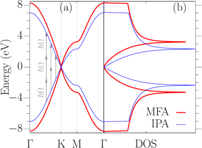
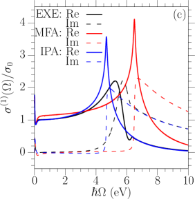
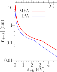
Figure 1: Effects of HF term on (a) the band structure, (b) the density of states, (c) the linear optical conductivity, and (d) the energy dependence of the dipole transition matrix elements between the two bands along the high symmetry lines K$\to$M$\to\Gamma$. The gray arrows in (a) indicate the resonant transitions by multiple photons.

In this paper the main quantity of interest is the current density, which is given by $\bm{J}(t)=(2\pi)^{-2}\int d\boldsymbol{k}\bm{J}_{\bm{k}}(t)$ with

$$\bm{J}_{\bm{k}}(t) =-e\sum_{\alpha\beta}{\bm{v}}_{\beta\alpha\bm{k}}(t){\rho}_{\alpha\beta\bm{k}}(t)\,,$$ (9)

$${\bm{v}}_{\alpha\beta\bm{k}}(t) =\frac{1}{i\hbar}\left\{(\bm{\tau}_{\alpha}-\bm{\tau}_{\beta}+i\bm{\nabla}_{\bm{k}})\left[{H}_{\alpha\beta(\bm{k}+e\bm{A}(t)/\hbar)}^{0}\right.\right.$$

$$\left.\left.+{H}_{\alpha\beta\bm{k}}^{\text{HF}}(t)\right]\right\}\,.$$ (10)

III Results

In our numerical calculation, we adopt the parameters $\gamma_{0}=2.34$ eV, $U=8.29$ eV, $\hbar/\Gamma=20$ fs, $\mu=0$ eV, $T=300$ K, and divide the Brillouin zone into a $N\times N$ grid with $N=1500$; our main results are not very sensitive to the exact values of $\gamma_{0}$ and $U$. The time differential is discretized by a fourth-order Runge-Kutta method with a time step $0.05$ fs. We consider background dielectric constants $\epsilon$ varying between $2$ and $9$. The results are presented for three different approaches: the independent particle approximation (IPA, with $\lambda_{m}=\lambda_{e}=0$), the mean field approximation (MFA, with $\lambda_{m}=1$ and $\lambda_{e}=0$), and taking into account excitonic effects (EXE, with $\lambda_{m}=\lambda_{e}=1$).

We numerically calculate the current density for a periodic field $\bm{E}(t)=E_{0}\hat{\bm{x}}e^{-i\Omega t}+c.c.$, with $E_{0}=5\times 10^{6}$ V/m, in the time range $0\leq t\leq 300$ fs . Because the relaxation time is much shorter than $300$ fs, we can approximate the current density in the last period as $J_{x}(t)=\sum_{n}\left[J_{x}^{(n)}e^{-in\Omega t}+c.c\right]$. The linear conductivity can be obtained by $\sigma^{(1)}(\Omega)=J_{x}^{(1)}/E_{0}$, and the THG conductivity is obtained by $\sigma^{(3)}(\Omega)=J_{x}^{(3)}/E_{0}^{3}$. For THG, the photon energies is chosen in the range of $0.2\leq\hbar\Omega\leq 3.4$ eV.

Insight into the dynamics induced by the applied field can be gained by looking at the transition energy resolved conductivities, which are defined as

$$\sigma^{(n)}(\Omega,\epsilon_{t}) =\int\frac{d\bm{k}}{(2\pi)^{2}}\frac{J_{x;\bm{k}}^{(n)}}{E_{0}^{n}}\delta(\epsilon_{t}-(\varepsilon_{+\bm{k}}-\varepsilon_{-\bm{k}}))\,,$$ (11)

where $J_{x;\bm{k}}^{(n)}$ is the $n$th order Fourier transformation of $J_{x;\bm{k}}(t)$. They describe how the electronic states at a given transition energy $\epsilon_{t}$ contribute to the optical conductivity at a fundamental frequency $\Omega$. In the IPA and MFA approximations, $|\sigma^{(n)}(\Omega,\epsilon_{t})|$ exhibits a peak at $\epsilon_{t}=m\hbar\Omega$ for the $m$-photon resonant optical transition for $1\leq m\leq n$, as would be expected within a single-particle description. In Fig. 1 (a) we illustrate the electronic states for $m$-photon resonant transitions at $m=1,2,3$. With the inclusion of HF term, the energy shift of these peaks can be used to identify excitonic effects. Very generally, the conductivities are given by the integral over transition energies of these resolved quantities, $\sigma^{(n)}(\Omega)=\int d\epsilon_{t}\sigma^{(n)}(\Omega,\epsilon_{t})$.

III.1 Band structure and linear conductivity

Figure 1 (a) and (b) give the single particle band structure and density of states (DOS) in the IPA and the MFA for $\epsilon=3$. In the IPA, the dispersion is linear around the Dirac points with a Fermi velocity $v_{F}=\sqrt{3}a_{0}\gamma_{0}/2\hbar\approx 0.76\times 10^{6}$ m/s, and the DOS is also approximately linear in a large energy range between about $-1.5$ eV and $1.5$ eV. There are significant changes in the band structure as we move to the MFA. Our results are in line with a host of other calculations showing that the single particle bands deviate from linear dispersion Hwang et al. (2007). And even away from the Dirac points the Fermi velocity increases. The band energy at the M point increases from $2.34$ eV in the IPA to $3.25$ eV in the MFA, and the energy at the $\Gamma$ point also increases from $7$ eV in the IPA to $8.27$ eV in the MFA. The increase of these characteristic

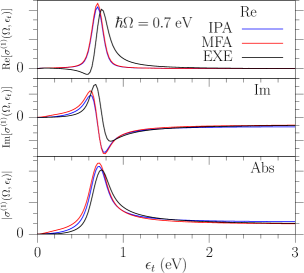
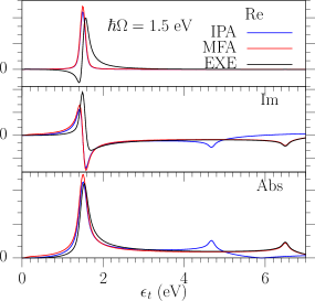
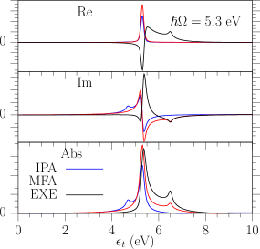
Figure 2: Transition energy resolved linear conductivity for different excitation frequency $\hbar\Omega=0.7$, $1.5$, and $5.3$ eV in the IPA, MFA, and EXE models. The values for the real part, the imaginary part, and the absolute values are presented.

energies by the HF term shows behavior similar to the effects of GW corrections in gapped semiconductors. Although both the IPA and MFA are single-particle approximations, their different band structures result in a clear difference between their predicted linear optical conductivities, as shown in Fig. 1(c). The MFA corrections to the dispersion also enhance the real parts of the linear conductivity for photon energies less than $2.5$ eV. The enhancement is a joint effect involving the enhanced dipole matrix elements shown in Fig. 1 (d) and the decreased DOS shown in Fig. 1 (b), and the former dominates. The result shows how the MFA modifies the single particle electronic states. When the photon energy matches the optical transition energy at the $M$ point, the real part of the conductivity shows a very sharp peak in both the IPA and MFA, induced by the van Hove singularity at the $M$ point. With the further inclusion of excitonic effects, the resulting linear conductivity in the EXE exhibits three main features: (1) The conductivity for $\hbar\omega<3$ eV is very close to the universal conductivity obtained in the IPA. (2) The singularity peak is shifted from a photon energy $6.5$ eV to $5.3$ eV, which indicates a strong excitonic effect around the $M$ point. The exciton binding energy is about $1.2$ eV, of the same order of magnitude for excitons in other 2D materials. (3) The broadened peak at the $M$ point, followed by a small dip, confirms the Fano resonance between the saddle excitons and continuum electron-hole states. These results agree qualitatively with an ab initio calculation Yang et al. (2009), which provides a good check of the reasonableness of our model. Roughly speaking, the linearity conductivity plot for EXE lies between that of IPA and MFA, indicating an interference between the mean field and excitonic contributions. We will see this kind of “undoing” of the mean field contributions by the excitonic contributions is even more pronounced when we consider the nonlinear response below.

In Fig. 2 we plot the transition energy resolved conductivity, $\sigma^{(1)}(\Omega,\epsilon_{t})$, for the excitation photon energies $\hbar\Omega=0.7$, $1.5$, and $5.3$ eV. For the single particle models (the IPA and MFA), a Lorentzian shape $\sigma^{(1)}(\Omega,\epsilon_{t})\propto i\left(\hbar\Omega-\epsilon_{t}+i\Gamma\right)^{-1}$ results. The real part of $\sigma^{(1)}(\Omega,\epsilon_{t})$, which corresponds to the absorption at each transition energy $\epsilon_{t}$, is always positive and localized around $\epsilon_{t}\sim\hbar\Omega$ with a broadening approximately determined by the relaxation parameter; this is as expected for a single particle theory. The difference between the IPA and the MFA is mainly due to the different optical transition matrix elements. For the imaginary part, the band structure and the density of states play important roles, with peaks around the singularity at the $M$ points ($\epsilon_{t}\approx 4.6$ eV for the IPA and 6.5 eV for the MFA). With the inclusion of the excitonic effects, $\sigma^{(1)}(\Omega,\epsilon_{t})$ deviates from its MFA behavior only around the peak at $\epsilon_{t}\approx\hbar\Omega$. For $\hbar\Omega=0.7$ and $1.5$ eV, the absolute value only changes slightly, but the mixture of the real and imaginary parts indicates a phase change of the optical transition matrix elements. Overall, excitonic effects are very weak for low photon energies, agreeing with the $ab$ $initio$ results. For $\hbar\Omega=5.3$ eV, the absolute value of $\sigma^{(1)}(\Omega,\epsilon_{t})$ include a significant contribution from the electronic states at the $M$ point for $\epsilon_{t}>\hbar\Omega$, showing the important role played by excitonic effects.

III.2 Third harmonic generation

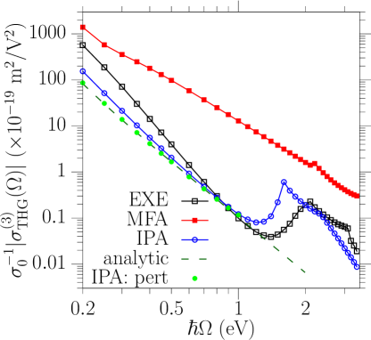
Figure 3: Effects of HF term on the nonlinear conductivity for third harmonic generation. The dotted curve gives the perturbative conductivity obtained by an analytic expression Cheng et al. (2015a); *Phys.Rev.B_93_39904_2016_Cheng; all the other three curves are obtained under a field $E_{0}=5\times 10^{6}$ V/m. The blue (red) curves are the results obtained from the single particle band structure with (without) HF corrections, and the black curves are obtained with the excitonic effects. The green dots are obtained using a field $E_{0}=10^{6}$ V/m.

We now turn to THG, the conductivities of which are plotted in Fig. 3 for IPA, MFA, and EXE. We first look at the spectra in the IPA. The absolute value of conductivity decreases with the photon energy, approximately following a power law $\propto\Omega^{-n_{0}}$ with $n_{0}\sim 4.4$, and reaches a minimum at $\hbar\Omega\approx 1.2$ eV; then it increases to a maximum at $\hbar\Omega\sim 1.6$ eV, and decreases again afterwards. This spectrum is very similar to perturbative results in literature Cheng et al. (2014); Liu et al. (2017). Ignoring relaxation, the analytic perturbative conductivity Cheng et al. (2015a); *Phys.Rev.B_93_39904_2016_Cheng gives $\sigma_{\text{THG}}\propto\Omega^{-4}$ for low photon energies, shown in Fig. 3 as a dashed curve. Our numerical results give a faster decay ($n_{0}>4$) because the simulation field strength $E_{0}=5\times 10^{6}$ V/m is slightly beyond the perturbative limit. Therefore saturation effects start to play a role, and they enhance the THG due to the extra optically excited carriers from the one-photon absorption Cheng et al. (2015b). As might be expected, the saturation is more important at low photon energy, where the saturation intensity is lower. The perturbative limit is obtained for a weaker field $E_{0}=10^{6}$ V/m, as shown by the green filled dots in Fig. 3, which agree with the analytic results very well. Because a much longer simulation time for this weak field is required, we keep our other calculations using $E_{0}=5\times 10^{6}$ V/m. The peak around $1.6$ eV is induced by the three photon resonant transition at the van Hove singularity point. This is consistent with an analytic perturbative result Liu et al. (2017).

When the Coulomb interaction is included at the level of MFA, the spectra are obviously different, shown as filled red squares in Fig. 3. For the calculated photon energies, the values in the MFA are orders of magnitude larger than those in the IPA, mirroring the change in the linear conductivity as we move from IPA to MFA, although the increase is much greater here. Except for a very weak peak around $\hbar\Omega\approx 2.2$ eV, which corresponds to the three photon resonant transition at the $M$ point, the whole spectrum follows a power law $\propto\Omega^{-n_{m}}$ with $n_{m}\approx 3$ for $\hbar\Omega<3.4$ eV. When the excitonic effects are included, the THG conductivity again changes dramatically, as shown in black square in Fig. 3. At low photon energies, $\hbar\Omega<1$ eV, the THG shows a different scaling with $\Omega$ than seen in either the IPA or the MFA, scaling as $\Omega^{-n_{e}}$ with $n_{e}\sim 5.5$; compared to the IPA results, the EXE are enhanced by about 3 times at $\hbar\Omega=0.2$ eV, but reduced about 20% at $\hbar\Omega=1$ eV. When the photon energy increases, a peak appears at $\hbar\omega\approx 2.1$ eV, which is the same energy for the weak peak appearing in MFA. In brief, the Coulomb interaction affects THG mainly in the following aspects: (1) THG in MFA is orders of magnitude larger than that in IPA. The increase is even much larger than that calculated for the linear response. Therefore the details of the band structure are very important for understanding the optical nonlinearity. (2) The further inclusion of EXE can bring the THG very close to the results in IPA, showing a strong interference between the mean field contribution and the excitonic contribution. (3) At low photon energies, the Coulomb interaction changes the photon energy dependence, with the power index changing from $n_{0}=4.4$ in the IPA to $n_{m}=3$ in the MFA and $n_{e}=5.5$ in the EXE. (4) For the EXE spectra, the three-photon resonance with the $M$ point gives a peak at $\hbar\Omega\approx 2.1$ eV. This energy does not correspond to the one third of the $M$ point exciton energy ( $5.3\text{~{}eV}/3\sim 1.8$ eV), but is very close to the one third of the $M$ point energy in the MFA ($6.5\text{~{}eV}/3\sim 2.16$ eV). The lack of an energy shift may indicate that the excitonic effects are not important for the three-photon resonance with the $M$ point. These four features indicate the importance of the Coulomb interaction on the THG in an intrinsic graphenem, where both (1) and (2) are very similar to the effects of Coulomb interaction on the linear optical response.

To gain some insight into these features, we calculate the transition-energy-resolved THG conductivity, shown in Fig. 4 for $\hbar\Omega=0.7$ eV, 1.5 eV, and 2.1 eV. In the single-particle approximations, the values of $|\sigma^{(3)}(\Omega,\epsilon_{t})|$ show three peak contributions located around transition energies $m\hbar\Omega$ with $m=1,2,3$, corresponding to the one-photon, two-photon, and three-photon resonant transitions. In IPA, the two-photon resonant transition destructively interferes with the one-photon and three-photon resonant transitions Cheng et al. (2014) (approximately corresponding to prefactors $-17,64,-45$), which results in a small THG conductivity. In the MFA, there are of course changes in the density of states and the dipole matrix elements that affect the THG, but as well the interference is also greatly changed due to the modification of the Dirac band structure. Although there is still some destructive interference between these transitions, the sign of the first peak in the MFA is changed compared to that in the IPA, the cancellation is not complete, and this leads to a larger THG response. As well, there is an additional peak located at zero energy. This peak has the same sign as the peak at $2\hbar\Omega$, and it is larger in the MFA than in the IPA. With the inclusion of excitonic effects, the transition energy distribution of the absolute values of THG becomes very similar to that of IPA, especially around the peak at $\epsilon_{t}=0$; simutaneously, an additional phase is introduced around each peak that changes both the real and imaginary parts. The results indicate that the interference between the mean field contributions and the excitonic effects also exists in the optical nonlinearity.

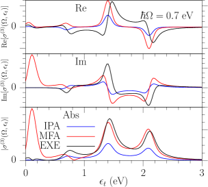
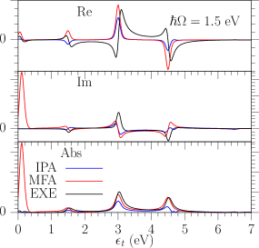
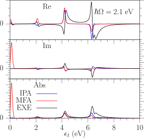
Figure 4: Transition energy resolved THG conductivity for fundamental photon energies $\hbar\Omega=0.7$ eV, 1.5 eV, and 2.1 eV.

For $\hbar\Omega=2.1$ eV, the transition energy resolved spectra shows that the resonant peaks locate around $\epsilon_{t}\sim m\hbar\Omega$, which are similar to the dependence in the single-particle approximation. This confirms that excitonic effects play a minor role for the peak around $\hbar\Omega\approx 2.1$ eV in Fig. 3.

III.3 Substrate effects

Because of the complexity of the nonlinear optical response of graphene, it is easy to reveal the consequences of many-body effects by changing the substrate, or more generally the environment, which is very effective in tuning the interaction strength of the Coulomb interaction Yadav et al. (2015). In Fig. 5 we show how the background dielectric constant $\epsilon$ affects the THG. The Coulomb interaction is inversely proportional to $\epsilon$, and thus a large background dielectric constant corresponds to a weak interaction; the limit $\epsilon\to\infty$ corresponds to no Coulomb interaction.

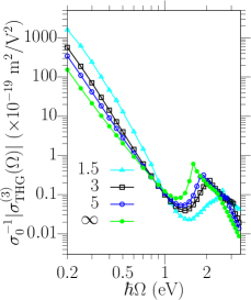
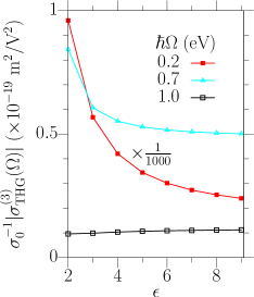
Figure 5: Effects of substrate dielectric constant $\epsilon$ on THG conductivity. (a) The spectrum of THG conductivity for different $\epsilon$, (b) The $\epsilon$ of THG conductivity for three photon energy $\hbar\Omega=0.2$, $0.7$, and $1.0$ eV. The results for $0.2$ eV are scaled by $10^{-3}$.

When $\epsilon$ increases, the THG conductivity decreases for photon energies $\hbar\Omega$ less than about $0.8$ eV, and the power index $n$ for $\sigma^{(3)}\propto\Omega^{-n}$ also decreases. But for photon energies $\hbar\Omega$ larger than about $0.8$ eV, the THG conductivity increases; the peak corresponding to the resonant three-photon transition at the $M$ point is shifted to a lower photon energy, because the energy renormalization decreases with the strength of the Coulomb interaction. The THG conductivity is more sensitive to the substrate dielectric constant at lower photon energies, and it can change over one order of magnitude for $\hbar\Omega=0.2$ eV when $\epsilon$ changes from $2$ to $\infty$.

IV Conclusion

We have theoretically investigated the effects of Coulomb interaction on third harmonic generation of undoped graphene in the unscreened Hartree-Fock approximation, with the inclusion of mean field energy correctionS and excitonic effects. Although there are no bound excitons formed in gapless graphene, the Coulomb interaction still affects the third harmonic generation significantly. We find that the Coulomb interaction can increase the amplitude of third harmonic generation at low photon energy, and decrease it at high photon energy. Despite the fact that saddle point excitons lead to a large energy shift of the resonant peak in linear absorption, they leave no energy fingerprint on the three-photon resonance in third harmonic generation. The underlying physics can be understood by the inclusion of the Coulomb interaction step by step. At the level of mean field approximation, the Coulomb interaction greatly modifies the single particle band structure, which leads to an enhancement of the third harmonic generation by around two orders of magnitude compared to the results obtained without Hartree-Fock term. However, with the full inclusion of the Hartree-Fock term, this large enhancement is largely cancelled, except for the Coulomb-induced changes of the power scaling. Therefore, there is a very strong interference between the contributions from the mean field energy correction and excitonic effects. We found these effects could be revealed experimentally by changing the background dielectric constant, leading to changes both in the absolute value of the third harmonic generation coefficient and in its frequency dependence. The strength of the modifications due to changes in the environment is very sensitive to the fundamental frequency, and a stronger dependence on the environment dielectric constant can be found at lower incident photon energy. Therefore, the strong dependence of third harmonic generation on the Coulomb interaction may provide a new optical tool for studying the many-body effect in graphene.

For undoped graphene, our results show that the Coulomb interaction can significantly modify third harmonic generation at low frequencies. Thus it may be important as well in other nonlinear optical phenomena involving small frequencies, such as degenerate four wave mixing, coherent current injection, Kerr effects and two-photon absorption, current induced second order optical nonlinearity, and jerk current Cheng et al. (2019). For doped graphene, where dynamic screening should be important, the unscreened Hartree-Fock approximation may be not adequate. Calculations of the optical nonlinearity in that material exhibit many resonances, arising whenever any photon energy involved matches the gap induced by a nonzero chemical potential. How the Coulomb interaction affects these resonances is an important but unexplored problem in understanding the physics of the optical nonlinearity in graphene.

Appendix A The derivation of the equation of motion

We start with a tight binding Hamiltonian $\hat{H}=\hat{H}_{0}+\hat{H}_{c}+e\bm{E}(t)\cdot\hat{\bm{r}}$ with

$$\hat{H}_{0} =\sum_{i\alpha,j\beta,\sigma}\gamma_{i-j,\alpha\beta}a_{i\alpha\sigma}^{{\dagger}}a_{j\beta\sigma}\,,$$ (12)

$$\hat{H}_{c} =\frac{1}{2}\sum_{{i\alpha\sigma_{1}\atop j\beta\sigma_{2}}}V_{i-j,\alpha\beta}a_{i\alpha\sigma_{1}}^{{\dagger}}a_{j\beta\sigma_{2}}^{{\dagger}}a_{j\beta\sigma_{2}}a_{i\alpha\sigma_{1}}\,,$$ (13)

$$\hat{\bm{r}} =\sum_{i\alpha\sigma}\bm{R}_{i\alpha}a_{i\alpha\sigma}^{{\dagger}}a_{i\alpha\sigma}\,.$$ (14)

Here $a_{i\alpha\sigma}$ is an annihilation operator of an electronic $p_{z}$ orbital with a spin $\sigma$ ($=\uparrow,\downarrow)$ at the site $\bm{R}_{i\alpha}=\bm{R}_{i}+\bm{\tau}_{\alpha}$, where $i=(n_{i},m_{i})$ is an abbreviated notation for $\bm{R}_{i}=n_{i}\bm{a}_{1}+m_{i}\bm{a}_{2}$. The term $\hat{H}_{0}$ gives the unperturbated tight binding Hamiltonian. In this paper, we use the parameters

$$\gamma_{i,AB} =-\gamma_{0}[\delta_{i,(0,0)}+\delta_{i,(1,0)}+\delta_{i,(0,1)}]\,,$$ (15)

$$\gamma_{i,BA} =-\gamma_{0}[\delta_{i,(0,0)}+\delta_{i,(-1,0)}+\delta_{i,(0,-1)}]\,.$$ (16)

We treat the Coulomb interaction $\hat{H}_{c}$ at the level of Hartree-Fock approximation, and take

$$\hat{H}_{c} \rightarrow\sum_{{i\alpha\sigma_{1}\atop j\beta\sigma_{2}}}V_{i-j,\alpha\beta}\left[\langle a_{i\alpha\sigma_{1}}^{{\dagger}}a_{i\alpha\sigma_{1}}\rangle a_{j\beta\sigma_{2}}^{{\dagger}}a_{j\beta\sigma_{2}}\right.$$

$$\left.-\langle a_{i\alpha\sigma_{1}}^{{\dagger}}a_{j\beta\sigma_{2}}\rangle a_{j\beta\sigma_{2}}^{{\dagger}}a_{i\alpha\sigma_{1}}\right]\,.$$ (17)

The constant energy shift in this approximation has been ignored. The notation $\langle P\rangle$ stands for the statistical average of the operator $P$ over the ground state. Considering a paramagnetic ground state in extended graphene, the term $\langle a_{i\alpha\sigma_{1}}^{{\dagger}}a_{j\beta\sigma_{2}}\rangle$ should only be a function of $i-j$ due to the translational symmetry. Then the first term can be seen to be a simple energy shift. By ignoring the spin we get an effective Hamiltonian as

$$\hat{H}_{\text{eff}}(t)=\sum_{i\alpha j\beta}\left[\gamma_{i-j,\alpha\beta}+\overline{H}_{i-j,\alpha\beta}^{\text{HF}}\right]a_{i\alpha}^{{\dagger}}a_{j\beta}+e\bm{E}(t)\cdot\hat{\bm{r}}\,,$$ (18)

with

$$\overline{H}_{i-j,\alpha\beta}^{\text{HF}}=-V_{i-j,\alpha\beta}\langle a_{j\beta}^{{\dagger}}a_{i\alpha}\rangle\,.$$ (19)

In this work, we describe the dynamics of the system by a density matrix $\overline{\rho}_{i-j,\alpha\beta}(t)=\langle a_{j\beta}^{{\dagger}}(t)a_{i\alpha}(t)\rangle$, with $a_{i\alpha}(t)$ being the operator $a_{i\alpha}$ in Heisenburg representation. In the Hartree-Fock approximation, it satisfies the equation of motion

$$i\hbar\partial_{t}\overline{\rho}_{i;\alpha\beta}(t) =\sum_{j}[\gamma_{i-j}+\overline{H}_{i-j}^{\text{HF}},\overline{\rho}_{j}(t)]_{\alpha\beta}$$

$$+e\bm{E}(t)\cdot(\bm{R}_{i}+\bm{\tau}_{\alpha}-\bm{\tau}_{\beta})\overline{\rho}_{i;\alpha\beta}(t)$$

$$-i\Gamma[\overline{\rho}_{i;\alpha\beta}(t)-\overline{\rho}_{i;\alpha\beta}^{0}]\,.$$ (20)

In the commutator, $\gamma_{i}$, $H_{i}^{\text{HF}}$, and $\overline{\rho}_{i}(t)$ are treated as matrices with elements determined by the indexes $\alpha\beta$. The last term models the relaxation process with one phenomenological energy parameter $\Gamma$, and $\rho_{i;\alpha\beta}^{0}$ gives the equilibrium distribution including the Hartree-Fock effects. The velocity operator is given by $\hat{\bm{v}}=(i\hbar)^{-1}[\hat{\bm{r}},\hat{H}_{\text{eff}}(t)]=\sum_{ij\alpha\beta}\bm{v}_{i-j,\alpha\beta}a_{i\alpha}^{{\dagger}}a_{j\beta}$ with

$$\bm{v}_{j,\alpha\beta} =(i\hbar)^{-1}(\bm{R}_{j}+\bm{\tau}_{\alpha}-\bm{\tau}_{\beta})\left(\gamma_{j,\alpha\beta}+\overline{H}_{j;\alpha\beta}^{\text{HF}}\right)\,.$$ (21)

Then the current density can be calculated through

$$\bm{J}(t)=-e\sum_{j\alpha\beta}\bm{v}_{j,\alpha\beta}\rho_{-j;\beta\alpha}(t)\,.$$ (22)

After Fourier transform of the index $i$ to wave vectors $\bm{k}$, i.e. $\gamma_{i}\to H_{\bm{k}}^{0}$, $\overline{H}_{j}^{\text{HF}}\to H_{\bm{k}}^{\text{HF}}$, $\overline{\rho}_{i}\to\rho_{\bm{k}}$, and changing to the moving frame, we get the equations in the main text.

References

- Kira and Koch (2006) M. Kira and S. Koch, Prog. Quantum Electron. 30, 155 (2006).
- (2) S.G. Louie, ”Chapter 2 Predicting Materials and Properties: Theory of the Ground and Excited State”, in ”Conceptual Foundations of Materials - A Standard Model for Ground- and Excited-State Properties” (Elsevier, 2006) pp. 9-53.
- Hwang and Das Sarma (2008) E. H. Hwang and S. Das Sarma, Phys. Rev. B 77, 081412 (2008).
- Grönqvist et al. (2012) J. Grönqvist, T. Stroucken, M. Lindberg, and S. Koch, Euro. Phys. J. B 85, 395 (2012).
- Yadav et al. (2015) P. Yadav, P. K. Srivastava, and S. Ghosh, Nanoscale 7, 18015 (2015).
- Yang et al. (2009) L. Yang, J. Deslippe, C.-H. Park, M. L. Cohen, and S. G. Louie, Phys. Rev. Lett. 103, 186802 (2009).
- Jung and MacDonald (2011) J. Jung and A. H. MacDonald, Phys. Rev. B 84, 085446 (2011).
- Katsnelson (2008) M. I. Katsnelson, Europhys. Lett. 84, 37001 (2008).
- Mak et al. (2011) K. F. Mak, J. Shan, and T. F. Heinz, Phys. Rev. Lett. 106, 046401 (2011).
- Mak et al. (2014) K. F. Mak, F. H. da Jornada, K. He, J. Deslippe, N. Petrone, J. Hone, J. Shan, S. G. Louie, and T. F. Heinz, Phys. Rev. Lett. 112, 207401 (2014).
- Malic et al. (2011) E. Malic, T. Winzer, E. Bobkin, and A. Knorr, Phys. Rev. B 84, 205406 (2011).
- Avetissian and Mkrtchian (2018) H. K. Avetissian and G. F. Mkrtchian, Phys. Rev. B 97, 115454 (2018).
- Zhang et al. (2019) Y. Zhang, D. Huang, Y. Shan, T. Jiang, Z. Zhang, K. Liu, L. Shi, J. Cheng, J. E. Sipe, W.-T. Liu, and S. Wu, Phys. Rev. Lett. 122, 047401 (2019).
- Jiang et al. (2018) T. Jiang, D. Huang, J. Cheng, X. Fan, Z. Zhang, Y. Shan, Y. Yi, Y. Dai, L. Shi, K. Liu, C. Zeng, J. Zi, J. E. Sipe, Y.-R. Shen, W.-T. Liu, and S. Wu, Nat. Photon. 12, 430 (2018), and references therein.
- Alexander et al. (2017) K. Alexander, N. A. Savostianova, S. A. Mikhailov, B. Kuyken, and D. V. Thourhout, ACS Photon. 4, 3039 (2017).
- Soavi et al. (2018) G. Soavi, G. Wang, H. Rostami, D. G. Purdie, D. De Fazio, T. Ma, B. Luo, J. Wang, A. K. Ott, D. Yoon, S. A. Bourelle, J. E. Muench, I. Goykhman, S. Dal Conte, M. Celebrano, A. Tomadin, M. Polini, G. Cerullo, and A. C. Ferrari, Nat. Nano. 13, 583 (2018).
- Yoshikawa et al. (2017) N. Yoshikawa, T. Tamaya, and K. Tanaka, Science 356, 736 (2017).
- Al-Naib et al. (2014) I. Al-Naib, J. E. Sipe, and M. M. Dignam, Phys. Rev. B 90, 245423 (2014).
- Baudisch et al. (2018) M. Baudisch, A. Marini, J. D. Cox, T. Zhu, F. Silva, S. Teichmann, M. Massicotte, F. Koppens, L. S. Levitov, F. J. G. de Abajo, and J. Biegert, Nat. Commun. 9, 1018 (2018).
- Bonaccorso et al. (2010) F. Bonaccorso, Z. Sun, T. Hasan, and A. C. Ferrari, Nat. Photon. 4, 611 (2010).
- Sun et al. (2016) Z. Sun, A. Martinez, and F. Wang, Nat. Photon. 10, 227 (2016).
- Autere et al. (2018) A. Autere, H. Jussila, Y. Dai, Y. Wang, H. Lipsanen, and Z. Sun, Adv. Mater. 30, 1705963 (2018).
- Mikhailov (2007) S. A. Mikhailov, Europhys. Lett. 79, 27002 (2007).
- Hendry et al. (2010) E. Hendry, P. J. Hale, J. Moger, A. K. Savchenko, and S. A. Mikhailov, Phys. Rev. Lett. 105, 097401 (2010).
- Gu et al. (2012) T. Gu, N. Petrone, J. F. McMillan, A. van der Zande, M. Yu, G. Q. Lo, D. L. Kwong, J. Hone, and C. W. Wong, Nat. Photon. 6, 554 (2012).
- Vermeulen et al. (2016) N. Vermeulen, D. Castelló-Lurbe, J. Cheng, I. Pasternak, A. Krajewska, T. Ciuk, W. Strupinski, H. Thienpont, and J. Van Erps, Phys. Rev. Appl. 6, 044006 (2016).
- Vermeulen et al. (2018) N. Vermeulen, D. Castelló-Lurbe, M. Khoder, I. Pasternak, A. Krajewska, T. Ciuk, W. Strupinski, J. Cheng, H. Thienpont, and J. Van Erps, Nat. Commun. 9, 2675 (2018).
- Cheng et al. (2014) J. L. Cheng, N. Vermeulen, and J. E. Sipe, New J. Phys. 16, 053014 (2014).
- Cheng et al. (2016a) J. L. Cheng, N. Vermeulen, and J. E. Sipe, New J. Phys. 18, 029501 (2016a).
- Cheng et al. (2015a) J. L. Cheng, N. Vermeulen, and J. E. Sipe, Phys. Rev. B 91, 235320 (2015a).
- Cheng et al. (2016b) J. L. Cheng, N. Vermeulen, and J. E. Sipe, Phys. Rev. B 93, 039904 (2016b).
- Cheng et al. (2015b) J. L. Cheng, N. Vermeulen, and J. E. Sipe, Phys. Rev. B 92, 235307 (2015b).
- Mikhailov (2016) S. A. Mikhailov, Phys. Rev. B 93, 085403 (2016).
- Jiang et al. (2007) J. Jiang, R. Saito, G. G. Samsonidze, A. Jorio, S. G. Chou, G. Dresselhaus, and M. S. Dresselhaus, Phys. Rev. B 75, 035407 (2007).
- Note (1) For graphene embedded inside two different materials, the background dielectric constant is the average of the dielectric constants. Because the interaction is mainly through the electric force outside of the graphene plane, the screening from the graphene electrons is ignored.
- Hwang et al. (2007) E. H. Hwang, B. Y.-K. Hu, and S. Das Sarma, Phys. Rev. Lett. 99, 226801 (2007).
- Stroucken et al. (2012) T. Stroucken, J. H. Grönqvist, and S. W. Koch, J. Opt. Soc. Am. B 29, A86 (2012).
- Stroucken et al. (2011) T. Stroucken, J. H. Grönqvist, and S. W. Koch, Phys. Rev. B 84, 205445 (2011).
- (39) Hartmut Haug and Antti-Pekka Jauho, Quantum Kinetics in Transport and Optics of Semiconductors (Springer, Berlin, 2007).
- Note (2) This work considers the third harmonic generation in the weak field regime, thus the use of a periodic field follows the standard perturbative treatment, which should be suitable in experiments where the pulse duration is much longer than the relaxation timeCheng et al. (2015b)..
- Liu et al. (2017) Z. Liu, C. Zhang, and J. C. Cao, Phys. Rev. B 96, 035206 (2017).
- Cheng et al. (2019) J. L. Cheng, J. E. Sipe, S. W. Wu, and C. Guo, APL Photonics 4, 034201 (2019).