Fano effect on the neutron elastic scattering by open-shell nuclei

Abstract

By focusing on the asymmetric shape of cross section, we analyze the pairing effect on the partial wave components of cross section for neutron elastic scattering off stable and unstable nuclei within the Hartree-Fock-Bogoliubov (HFB) framework. Explicit expressions for Fano parameters $q_{lj}$ and $\epsilon_{lj}$ have been derived and the pairing effects have been analyzed in term of these parameters, and the Fano effect was found on the neutron elastic scattering off the stable nucleus in terms of the pairing correlation. Fano effect was appeared as the asymmetric line-shape of the cross section caused by the small absolute value of $q_{lj}$ due to the small pairing effect on the deep-lying hole state of the stable nucleus. In the case of the unstable nuclei, the large $q_{lj}$ value is expected because of the small absolute value of the Fermi energy. The quasiparticle resonance with the large $q_{lj}$ forms the Breit-Wigner type shape in the elastic scattering cross section.

I Introduction

The Fano effect fano has been known as an universal quantum phenomenon in which the transition probability becomes a characteristic asymmetric shape caused by the interference effect due to the correlation between discrete states (or resonance) and continuum. Many examples of Fano effect can be found in physics even though the mechanism is quite different for each example. The Raman scattering raman ; raman2 , the photoelectric emission photoe , photoionization atom , the photoabsorption photoabs and the neutron scattering nscat are examples which have been known in spectroscopy. Recently, in atomic and condensed matter physics, experimental research to control the Fano effect has been started ott ; ryu in order to investigate the detailed dynamical system of the Fano effect. Also in nuclear physics, some observed resonances have been reported as the candidate of the Fano resonance orrigo ; orrigo2 , however, there was no detailed study/analysis in terms of the Fano parameters, so far.

In nuclear physics, sharp resonances found in the experimental data of ¹⁵N(⁷Li,⁷Be)¹⁵C reaction have been analyzed by using the channel-coupling equation, and introduced as the candidates for the Fano resonance orrigo . Another candidate for the Fano resonance in nuclei is the quasiparticle resonance (or pair resonance) due to the particle-hole configuration mixing caused by the pairing effect at the ground state of the open shell nuclei. The experimental cross section data of d(⁹Li,¹⁰Li)p reaction has been analyzed in terms of the effect of the pair resonance basing on the HFB formalism orrigo2 . Despite mentioning the possibility that these two candidates introduced in previous studies are Fano effect, there was no detailed study on Fano parameters.

The aim of this study is to organize the Fano formula for the neutron elastic scattering on the open shell nuclei with the help of the Jost function formalism jost based on the HFB jost-hfb , and we shall discuss the role of the Fano parameters for the quasiparticle resonances seen in the partial cross section of the neutron elastic scattering. Because characteristic asymmetric shapes of the cross sections have been shown as the numerical results obtained by the HFB framework jost-hfb .

Firstly, we divide the Jost function into two parts: the scattering part and the pairing part. The Gell-Mann-Goldberger relation for the T-matrix (expressed by the Jost function) has been obtained based on the HFB approach. Secondly, we derive the explicit expressions of the Fano parameters $q$ and $\epsilon$ for the neutron elastic scattering by open-shell nuclei within the HFB framework. Finally, the role of the Fano parameters has been analyzed in comparison with the square of the T-matrix plotted as a function of the incident energy of neutron.

II Method

II.1 Gell-Mann-Goldberger relation in HFB

The Jost function based on the HFB jost-hfb can be divided as

$$\left(\mathcal{J}_{lj}^{(\pm)}(E)\right)_{s1}$$

$$=\delta_{s1}J_{0,lj}^{(\pm)}(k_{1}(E))$$

$$\mp\frac{2m}{\hbar^{2}}\frac{k_{1}(E)}{i}\int dr\varphi_{0,lj}^{(\pm)}(r;k_{1}(E))\Delta(r)\varphi_{2,lj}^{(rs)}(r;E),$$ (1)

using the Hartree-Fock (HF) solutions $\varphi_{0,lj}^{(\pm)}(r;k_{1}(E))$ which satisfy the out-going/in-coming boundary conditions, and $\varphi_{2,lj}^{(rs)}(r;E)$ is the lower component of the HFB solution which is regular at the origin $r=0$, where $E$ is the quasiparticle energy and $k_{1}(E)$ is the momentum defined by $k_{1}(E)=\sqrt{\frac{2m}{\hbar^{2}}(\lambda+E)}$ with the Fermi energy $\lambda(<0)$. $J_{0,lj}^{(\pm)}(k_{1}(E))$ is the HF Jost function given by

$$J_{0,lj}^{(\pm)}(k_{1}(E))$$

$$=1$$

$$\mp\frac{2m}{\hbar^{2}}\frac{k_{1}(E)}{i}\int drrh^{(\pm)}_{l}(k_{1}(E)r)U_{lj}(r)\varphi_{0,lj}^{r}(r;k_{1}(E)),$$

(2)

$U_{lj}(r)$ and $\Delta(r)$ are the HF mean field and the pair potential, respectively. We adopt the same Woods-Saxon form and their parameters as jost-hfb for the numerical calculation. $\varphi_{0,lj}^{r}(r;k_{1}(E))$ is the regular solution of the HF equation. $\varphi_{0,lj}^{r}(r;k_{1}(E))$ and $\varphi_{0,lj}^{(\pm)}(r;k_{1}(E))$ are connected by using $J_{0,lj}^{(\pm)}(k_{1}(E))$ as

$$\varphi_{0,lj}^{r}(r;k_{1}(E))=\frac{1}{2}\left[J_{0,lj}^{(+)}(k_{1}(E))\varphi_{0,lj}^{(-)}(r;k_{1}(E))\right.$$

$$\hskip 28.45274pt\left.+J_{0,lj}^{(-)}(k_{1}(E))\varphi_{0,lj}^{(+)}(r;k_{1}(E))\right].$$ (3)

From Eqs.(1) and (3), we derive

$$\left(\mathcal{J}_{lj}^{(-)}(E)\right)_{s1}J_{0,lj}^{(+)}(k_{1}(E))-\left(\mathcal{J}_{lj}^{(+)}(E)\right)_{s1}J_{0,lj}^{(-)}(k_{1}(E))$$

$$=\frac{2m}{\hbar^{2}}\frac{2k_{1}(E)}{i}\int dr\varphi_{0,lj}^{r}(r;k_{1}(E))\Delta(r)\varphi_{2,lj}^{(rs)}(r;E).$$ (4)

Applying the HFB T-matrix given by Eq. (60) in  jost-hfb and the HF T-matrix given by

$$T_{lj}^{(0)}(E)=\frac{i}{2}\left(\frac{J_{0,lj}^{(-)}(k_{1}(E))}{J_{0,lj}^{(+)}(k_{1}(E))}-1\right)$$

$$=\frac{2mk_{1}(E)}{\hbar^{2}}\int_{0}^{\infty}drrj_{l}(k_{1}(E)r)U_{lj}(r)\psi_{0,lj}^{(+)}(r;k_{1}(E))$$

$$=\frac{2mk_{1}(E)}{\hbar^{2}}\langle j_{l}(k_{1}(E))|U_{lj}|\psi_{0,lj}^{(+)}(k_{1}(E))\rangle.$$ (5)

to Eq.(4), we obtain

$$T_{lj}(E)-T_{lj}^{(0)}(E)$$

$$=\frac{2mk_{1}(E)}{\hbar^{2}}\int dr\psi_{0,lj}^{(+)}(r;k_{1}(E))\Delta(r)\psi_{2,lj}^{(+)}(r;E),$$ (6)

where $\psi_{0,lj}^{(\pm)}(r;k_{1}(E))=\varphi_{0,lj}^{r}(r;k_{1}(E))/J_{0,lj}^{(\pm)}(k_{1}(E))$ and $\psi_{2,lj}^{(+)}(r;E)$ is the lower component of the HFB scattering wave function jost-hfb .

Eq. (6) is the so-called “Gell-Mann-Goldberger relation” (two potential formula) gellmann ; Hussein in the HFB formalism. We can read that the right hand side of Eq. (6) represents the transition from the hole-like component (lower component) of the HFB scattering states to the HF scattering states caused by the pairing field $\Delta(r)$. The HFB scattering wave function $\psi_{lj}^{(+)}(r;E)=\begin{pmatrix}\psi_{1,lj}^{(+)}(r;E)\\ \psi_{2,lj}^{(+)}(r;E)\end{pmatrix}$ can be represented in the integral form as

$$\begin{pmatrix}\psi_{1,lj}^{(+)}(r;E)\\ \psi_{2,lj}^{(+)}(r;E)\end{pmatrix}=\begin{pmatrix}\psi_{0,lj}^{(+)}(r;k_{1}(E))\\ 0\end{pmatrix}$$

$$+\int dr^{\prime}\begin{pmatrix}\mathcal{G}_{lj}^{11}(r,r^{\prime};E)&\mathcal{G}_{lj}^{12}(r,r^{\prime};E)\\ \mathcal{G}_{lj}^{21}(r,r^{\prime};E)&\mathcal{G}_{lj}^{22}(r,r^{\prime};E)\end{pmatrix}$$

$$\hskip 10.0pt\times\begin{pmatrix}0&\Delta(r^{\prime})\\ \Delta(r^{\prime})&0\end{pmatrix}\begin{pmatrix}\psi_{0,lj}^{(+)}(r^{\prime};k_{1}(E))\\ 0\end{pmatrix},$$ (7)

using the HFB Green’s function given by $2\times 2$ matrix form fayans ; matsuo ; belyaev .

Inserting Eq. (7) into the r.h.s. of Eq. (6), one obtains

$$T_{lj}(E)-T_{lj}^{(0)}(E)$$

$$=\frac{2mk_{1}(E)}{\hbar^{2}}\int\int drdr^{\prime}$$

$$\times\psi_{0,lj}^{(+)}(r;k_{1}(E))\Delta(r)\mathcal{G}_{lj}^{22}(r,r^{\prime};E)\Delta(r^{\prime})\psi_{0,lj}^{(+)}(r^{\prime};k_{1}(E)).$$

(8)

Since it has been proved that $S_{lj}^{11}(E)$ satisfies the unitarity on the scattering states defined on the real axis of $E$ above the Fermi energy $-\lambda$ in  jost-hfb , $S_{lj}^{11}(E)$ can be expressed as $S_{lj}^{11}(E)=e^{2i\delta_{lj}(E)}$. (The quasiparticle energy $E$ is hereafter supposed to be on the scattering states.) Also $S_{lj}^{(0)}(E)$ can be expressed $S_{lj}^{(0)}(E)=e^{2i\delta_{lj}^{(0)}(E)}$ because of no absorption in $U_{lj}(r)$. Here, let us define a phase-shift as $\delta_{lj}^{(1)}\equiv\delta_{lj}-\delta_{lj}^{(0)}$ to define $T_{lj}^{(1)}\equiv-e^{i\delta_{lj}^{(1)}(E)}\sin\delta_{lj}^{(1)}(E)$, and it may be rather trivial that $T_{lj}(E)$, $T_{lj}^{(0)}(E)$ and $T_{lj}^{(1)}(E)$ are related by

$$T_{lj}(E) = T_{lj}^{(0)}(E)+T_{lj}^{(1)}(E)S_{lj}^{(0)}(E)$$ (10)

$$= T_{lj}^{(0)}(E)\left(1-iT_{lj}^{(1)}(E)\right)$$

$$+T_{lj}^{(1)}(E)\left(1-iT_{lj}^{(0)}(E)\right).$$

II.2 Fano parameters

In this paper, we analyze the pairing effect on the partial cross sections of $p_{1/2}$ with $\lambda=-8.0$ MeV and $d_{3/2}$ with $\lambda=-1.0$ MeV by using the same Woods-Saxon parameters for the numerical calculation as in Ref.  jost-hfb . Both resonances are the so-called hole-type resonances originated from the hole state resulting from the particle-hole (p-h) configuration mixing due to the pairing. As shown in Fig.6 of jost-hfb , there is only one hole state for both $p_{1/2}$ and $d_{3/2}$ at the no pairing limit.

In such cases, the Hartree-Fock Green function can be expressed as

$$G_{HF,lj}(r,r^{\prime};\epsilon(k))$$

$$=\frac{\phi_{h,lj}(r)\phi^{*}_{h,lj}(r^{\prime})}{\epsilon(k)-e_{h}}-i\frac{2mk}{\hbar^{2}}\psi_{0,lj}^{(+)}(r;k)\psi_{0,lj}^{(+)*}(r^{\prime};k)$$

$$+\frac{2m}{\hbar^{2}}\frac{2}{\pi}P\int_{0}^{\infty}dk^{\prime}k^{\prime 2}\frac{\psi_{0,lj}^{(+)}(r;k^{\prime})\psi_{0,lj}^{(+)*}(r^{\prime};k^{\prime})}{k^{2}-k^{\prime 2}},$$ (11)

by dividing the continuum part into the principal and other parts in the spectral representation. Here $\epsilon(k)=\frac{\hbar^{2}k^{2}}{2m}$.

Using Eq.(11), we obtain

$$\langle\phi_{h,lj}|\mathcal{G}_{lj}^{22}(E)|\phi_{h,lj}\rangle=\frac{1}{E-\lambda+e_{h}-F_{lj}(E)+i\Gamma_{lj}(E)/2},$$

(12)

$$F_{lj}(E)=\frac{2m}{\hbar^{2}}\frac{2}{\pi}P\int_{0}^{\infty}dk^{\prime}k^{\prime 2}\frac{|\langle\psi_{0,lj}^{(+)}(k^{\prime})|\Delta|\phi_{h,lj}\rangle|^{2}}{k^{2}_{1}(E)-k^{\prime 2}},$$ (13)

$$\Gamma_{lj}(E)/2=\frac{2mk_{1}(E)}{\hbar^{2}}|\langle\psi_{0,lj}^{(+)}(k_{1}(E))|\Delta|\phi_{h,lj}\rangle|^{2},$$ (14)

as an exact solution of the HFB Dyson equation for $\mathcal{G}_{lj}$.

Using Eqs. (8), (10) and (II.2), we derive

$$T_{lj}^{(1)}(E) = \frac{\Gamma_{lj}(E)/2}{E-\lambda+e_{h}-F_{lj}(E)+i\Gamma_{lj}(E)/2}.$$ (15)

This is the typical Breit-Wigner formula for the hole-type quasiparticle resonance. From this formula, we can notice that the hole state which satisfies $2\lambda-e_{h}-F_{lj}(E)>0$ can be observed as the quasiparticle resonance in the neutron elastic scattering cross section since the incident neutron energy $E_{i}$ is defined by $E_{i}=E+\lambda$.

One of the parameters introduced by U.Fano fano , $\epsilon_{lj}(E)$ is defined by

$$\epsilon_{lj}(E) = \frac{1-iT_{lj}^{(1)}(E)}{T_{lj}^{(1)}(E)}$$ (16)

$$= \frac{E-\lambda+e_{h}-F_{lj}(E)}{\Gamma_{lj}(E)/2}.$$ (17)

We notice that the quasiparticle resonance energy $E_{r}$ and the width $\Gamma_{lj}(E_{r})$ can be estimated as

$$\epsilon_{lj}(E=E_{r}) = 0,$$ (18)

$$\left.\frac{d\epsilon_{lj}(E)}{dE}\right|_{E=E_{r}} = \frac{2}{\Gamma_{lj}(E_{r})},$$ (19)

by using Eq.(17).

When $\langle\psi_{0,lj}^{(+)}(k_{1}(E))|\Delta|\phi_{h,lj}\rangle\neq 0$, we can obtain

$$1-iT_{lj}^{(0)}(E)$$

$$=\frac{\langle\psi_{0,lj}^{(+)}(k_{1}(E))|\Delta|\phi_{h,lj}\rangle-iT_{lj}^{(0)}(E)\langle\psi_{0,lj}^{(+)}(k_{1}(E))|\Delta|\phi_{h,lj}\rangle}{\langle\psi_{0,lj}^{(+)}(k_{1}(E))|\Delta|\phi_{h,lj}\rangle}$$

$$=\frac{\langle\psi_{0,lj}^{(+)}(k_{1}(E))|\Delta|\phi_{h,lj}\rangle-\langle j_{l}(k_{1}(E))|U_{lj}G^{*}_{HF,lj}\Delta|\phi_{h,lj}\rangle}{\langle\psi_{0,lj}^{(+)}(k_{1}(E))|\Delta|\phi_{h,lj}\rangle}$$

$$\hskip 10.0pt+\frac{2m}{\hbar^{2}}\frac{2}{\pi}P\int_{0}^{\infty}dk^{\prime}k^{\prime 2}$$

$$\hskip 20.0pt\times\frac{\langle j_{l}(k_{1}(E))|U_{lj}|\psi_{0,lj}^{(+)}(k^{\prime})\rangle\langle\psi_{0,lj}^{(+)}(k^{\prime})|\Delta|\phi_{h,lj}\rangle}{(k_{1}^{2}(E)-k^{\prime 2})\langle\psi_{0,lj}^{(+)}(k_{1}(E))|\Delta|\phi_{h,lj}\rangle},$$

(20)

by using Eqs.(5) and (11). Note that $\langle j_{l}(k_{1}(E))|U_{lj}|\phi_{h,lj}\rangle=0$ is also used.

Since $|\psi_{0,lj}^{(+)}(k)\rangle$ satisfies the Lippmann-Schwinger equation $|\psi_{0,lj}^{(+)}(k)\rangle=(1+G_{HF,lj}U_{lj})|j_{l}(k)\rangle$, we rewrite Eq.(20) as

$$1-iT_{lj}^{(0)}(E)=\frac{\langle j_{l}(k_{1}(E))|\Delta|\phi_{h,lj}\rangle+\displaystyle{\frac{2m}{\hbar^{2}}\frac{2}{\pi}P\int_{0}^{\infty}dk^{\prime}k^{\prime 2}\frac{\langle j_{l}(k_{1}(E))|U_{lj}|\psi_{0,lj}^{(+)}(k^{\prime})\rangle\langle\psi_{0,lj}^{(+)}(k^{\prime})|\Delta|\phi_{h,lj}\rangle}{k_{1}^{2}(E)-k^{\prime 2}}}}{\langle\psi_{0,lj}^{(+)}(k_{1}(E))|\Delta|\phi_{h,lj}\rangle}.$$ (21)

Using Eq.(21), another parameter $q_{lj}(E)$ is defined by

$$q_{lj}(E) = \frac{1-iT_{lj}^{(0)}(E)}{T_{lj}^{(0)}(E)}$$ (23)

$$=\frac{\langle\chi_{l}(k_{1}(E))|\mathcal{U}_{lj}|\Phi_{h,lj}\rangle}{T_{lj}^{(0)}(E)\langle\psi_{0,lj}^{(+)}(k_{1}(E))|\Delta|\phi_{h,lj}\rangle},$$

where

$$|\Phi_{h,lj}\rangle=\begin{pmatrix}|\Phi_{h,lj}^{(1)}\rangle\\ |\Phi_{h,lj}^{(2)}\rangle\end{pmatrix}$$

$$=\begin{pmatrix}\frac{2m}{\hbar^{2}}\frac{2}{\pi}P\int_{0}^{\infty}dk^{\prime}k^{\prime 2}\frac{|\psi_{0,lj}^{(+)}(k^{\prime})\rangle\langle\psi_{0,lj}^{(+)}(k^{\prime})|\Delta|\phi_{h,lj}\rangle}{k_{1}^{2}(E)-k^{\prime 2}}\\ |\phi_{h,lj}\rangle\end{pmatrix},$$ (24)

$$|\chi_{l}(k)\rangle=\begin{pmatrix}|j_{l}(k)\rangle\\ 0\end{pmatrix},\hskip 10.0pt\mathcal{U}_{lj}=\begin{pmatrix}U_{lj}&\Delta\\ \Delta&-U_{lj}\end{pmatrix}.$$ (25)

The upper component of $|\Phi_{h,lj}\rangle$ is originated from the admixture of a hole state and continuum due to the pairing. Note that, Eq. (23) is quite analogous to Eq. (20) in fano .

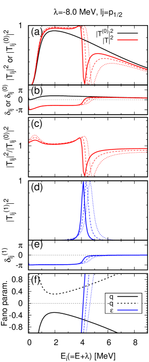
Figure 1: (Color online) The numerical results of square of T-matrix of the neutron elastic scattering, corresponding phase-shift, and the Fano parameters $q$ and $\epsilon$ for $p_{1/2}$ plotted as a function of the incident neutron energy $E_{i}(=E+\lambda)$ with $\lambda=-8.0$ MeV. See text for details.

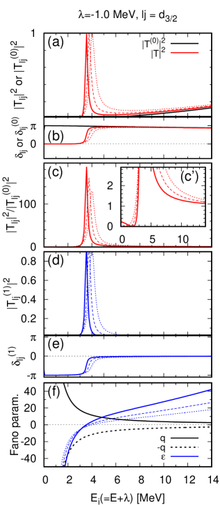
Figure 2: (Color online) Same with Fig.1 but for $d_{3/2}$ with $\lambda=-1.0$ MeV.

II.3 Fano formula

Applying Eqs. (16) and (23) to Eq.(10), it is rather easy to obtain

$$T_{lj}(E) = -e^{i\delta_{lj}^{(1)}(E)}\frac{q_{lj}(E)+\epsilon_{lj}(E)}{\sqrt{1+\epsilon^{2}_{lj}(E)}}T_{lj}^{(0)}(E).$$ (26)

Thus, we finally obtain the so-called Fano formula

$$\frac{|T_{lj}(E)|^{2}}{|T_{lj}^{(0)}(E)|^{2}} = \frac{(q_{lj}(E)+\epsilon_{lj}(E))^{2}}{1+\epsilon^{2}_{lj}(E)}.$$ (27)

Using Eqs. (23) and (14), we obtain a very similar formula to Eq. (22) of Ref. fano

$$q_{lj}^{2}(E)/2=\frac{\hbar^{2}k_{1}^{2}(E)}{2m}\frac{|\frac{2m}{\hbar^{2}}\frac{1}{\sqrt{k_{1}(E)}}\langle\chi_{l}(k_{1}(E))|\mathcal{U}_{lj}|\Phi_{h,lj}\rangle|^{2}}{|T_{lj}^{(0)}(E)|^{2}\Gamma_{lj}(E)}$$

. (28)

Since the resonance energy $E_{r}$ is determined by Eq. (18) and $\Gamma_{lj}(E_{r})$ is the width of the quasiparticle resonance, we obtain

$$\frac{|T_{lj}(E_{r})|^{2}}{|T_{lj}^{(0)}(E_{r})|^{2}}=q_{lj}^{2}(E_{r})$$ (29)

$$=\frac{|\frac{2m}{\hbar^{2}}\frac{1}{\sqrt{k_{1}(E_{r})}}\langle\chi_{l}(k_{1}(E_{r}))|\mathcal{U}_{lj}|\Phi_{h,lj}\rangle|^{2}}{|T_{lj}^{(0)}(E_{r})|^{2}\Gamma_{lj}(E_{r})/2E_{i}^{r}},$$ (30)

where $E_{i}^{r}=E_{r}+\lambda=\frac{\hbar^{2}k_{1}^{2}(E_{r})}{2m}$. The numerator of Eq.(30) is the transition probability to the “modified quasi-hole” state at the resonance $E_{r}$.

Therefore, $q_{lj}^{2}(E_{r})/2$ is regarded as the ratio of the transition probabilities to the “modified quasi-hole” state $|\Phi_{h,lj}\rangle$ and to a scaled width $\Gamma_{lj}(E_{r})/E_{i}^{r}$ of the HF continuum states $|\psi_{0,lj}^{(+)}\rangle$ at a quasiparticle resonance energy $E_{r}$.

As well known, the characteristic features of the Fano formula Eq. (27) are

1. The shape of $\left|\frac{T_{lj}(E)}{T_{lj}^{(0)}(E)}\right|^{2}$ approaches the Breit-Wigner shape at the limit $|q_{lj}(E)|\to\infty$.

2. $\left|\frac{T_{lj}(E)}{T_{lj}^{(0)}(E)}\right|^{2}$ becomes zero at the energy $E=E_{c}$ which satisfies $q_{lj}(E_{c})=-\epsilon_{lj}(E_{c})$.

Also the parameter $q_{lj}(E)$ causes the asymmetric shape of $\left|\frac{T_{lj}(E)}{T_{lj}^{(0)}(E)}\right|^{2}$ in $E$ as shown in Fig.1 of fano when the absolute value of $q_{lj}(E)$ is non-zero small value (see Fig. 1 of fano ), $q_{lj}(E)$ is, therefore, called “Fano asymmetry parameter” asymfano . Besides, it is clear from Eq.(15) that $|T_{lj}^{(1)}(E)|^{2}$ always keeps the shape of the Breit-Wigner formula if a quasiparticle resonance exists.

Table 1: The pairing gap dependence of $E_{r}$, $\Gamma_{lj}(E_{r})$, $q_{lj}(E_{r})$ and $E_{c}$ for $p_{1/2}$ with $\lambda=-8.0$ MeV and $d_{3/2}$ with $\lambda=-1.0$ MeV. The energies $E_{r}^{i}$ and $E_{c}^{i}$ defined by $E_{i}^{r}=E_{r}+\lambda$ and $E_{i}^{c}=E_{c}+\lambda$ are shown in parenthesis. The results are shown in units of MeV except $q_{lj}$, $q_{lj}$ is a dimensionless quantity.

	$p_{1/2}$				$d_{3/2}$
	($\lambda=-8.0$ MeV)				($\lambda=-1.0$ MeV)
$\langle\Delta\rangle$	$E_{r}$	$\Gamma_{lj}$	$q_{lj}$	$E_{c}$	$E_{r}$	$\Gamma_{lj}$	$q_{lj}$	$E_{c}$
	$(E_{i}^{r})$			$(E_{i}^{c})$	$(E_{i}^{r})$			$(E_{i}^{c})$
$2.0$	$12.14$	$0.28$	$-0.55$	$12.21$	$4.53$	$0.20$	$13.80$	$2.94$
	$(4.14)$			$(4.21)$	$(3.53)$			$(1.94)$
$2.5$	$12.37$	$0.42$	$-0.58$	$12.49$	$4.75$	$0.34$	$12.67$	$2.27$
	$(4.37)$			$(4.49)$	$(3.75)$			$(1.27)$
$3.0$	$12.65$	$0.56$	$-0.63$	$12.84$	$4.99$	$0.52$	$11.55$	$1.45$
	$(4.65)$			$(4.84)$	$(3.99)$			$(0.45)$

III Numerical analysis

Numerical results for $p_{1/2}$ with $\lambda=-8.0$ MeV and $d_{3/2}$ with $\lambda=-1.0$ MeV are shown in Figs.1 and 2, respectively, by adopting the Woods-Saxon potential for the mean field potential and pair potential with same parameters as jost-hfb .

In panel (a) of Figs. 1 and 2, the square of T-matrix $|T_{lj}|^{2}$ and $|T_{lj}^{(0)}|^{2}$ of the neutron elastic scattering are plotted as a function of the incident neutron energy $E_{i}(=E+\lambda)$ by red curves and black curve. The solid red curve shows $|T_{lj}|^{2}$ with $\langle\Delta\rangle=2.0$ MeV. The dashed and dotted curves are the same ones with $\langle\Delta\rangle=2.5$ and $3.0$ MeV, respectively. Corresponding phase shifts are shown in the panel (b). In panel (c), $|T_{lj}|^{2}/|T_{lj}^{(0)}|^{2}$ which is representative of the quantity of the Fano formula Eq.(27). We show $|T_{lj}^{(1)}|$ represented by Eq.(15) in the panel (d), and the corresponding phase shifts $\delta_{lj}^{(1)}$ are shown in the panel (e). The Fano parameters $q_{lj}$ and $\epsilon_{lj}$ are plotted by the solid black curve and the red curves in the panel (f). The dashed black curve represents $-q_{lj}$. The pairing dependence for all quantities in panels (b)-(f) is shown by solid, dashed and dotted curves (corresponding to $\langle\Delta\rangle=2.0,2.5$ and $3.0$ MeV) as well as panel (a). The values of $E_{r}$, $\Gamma_{lj}(E_{r})$, $q_{lj}(E_{r})$ and $E_{c}$ for $p_{1/2}$ with $\lambda=-8.0$ MeV and $d_{3/2}$ with $\lambda=-1.0$ MeV are shown in Table 1. It is confirmed that these values of $E_{r}$ and $\Gamma_{lj}(E_{r})$ matches with the zeros of the absolute values of the Jost function on the complex energy plane shown in jost-hfb .

In Fig. 1, there is a dip at $E_{i}^{c}(=E_{c}+\lambda)$ and asymmetric shape in $|T_{lj}|^{2}$(panel (a)) and $|T_{lj}|^{2}/|T_{lj}^{(0)}|^{2}$ (panel (c)). According to the characteristic of the Fano formula Eq.(27), this asymmetric shape is due to the small absolute value of $q_{lj}$ at the resonance energy $E_{r}$ as shown in panel (f) and Table 1. In the panel (d), $|T_{lj}^{(1)}|^{2}$ shows a typical Breit-Wigner resonance shape representing a hole-type quasiparticle resonance originates from a deep-lying hole state ($e_{p_{1/2}}=-19.71$ MeV) due to the pairing correlation. The typical behaviour of the phase shift for a resonance can be seen in the panel (e). In Fig. 2, there is a sharp resonance in the panels (a), (c) and (d). This resonance originates from a hole state at $e_{d_{3/2}}=-5.12$ MeV. According to the characteristic of the Fano formula Eq. (27), this is due to the large absolute value of $q_{lj}$ at the resonance energy $E_{r}$ as shown in a panel (f) and Table 1. The typical behaviour of the phase shift for a resonance can be seen in both panels (b) and (e).

In Table 1, one can see that the energies $E_{r}$ and $E_{c}$ are shifted to higher energy, and the width $\Gamma_{lj}(E_{r})$ becomes larger as the pairing gap $\langle\Delta\rangle$ increases. These are rather trivial pairing effects, because the energy shift $F_{lj}$ and width $\Gamma_{lj}$ are represented by Eqs.(13) and (14), and the pairing does not change the relative position between $E_{r}$ and $E_{c}$. However, the pairing effect on $q_{lj}(E_{r})$ is not so simple. In the case of $p_{1/2}$ with $\lambda=-8.0$ MeV, the absolute value of $q_{lj}(E_{r})$ increases as the pairing gap $\langle\Delta\rangle$ increases. On the other hand, the absolute value of $q_{lj}(E_{r})$ decreases as the pairing gap $\langle\Delta\rangle$ increases in the case of $d_{3/2}$ with $\lambda=-1.0$ MeV.

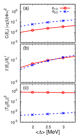
Figure 3: (Color online) The pairing gap $\langle\Delta\rangle$ dependence for the numerator of Eq.(30), the scaled width $\Gamma/E_{i}^{r}$ and $|T_{0}|^{2}$ are shown in panels (a), (b) and (c) respectively. The red solid and blue dashed curves represent $p_{1/2}$ with $\lambda=-8.0$ MeV and $d_{3/2}$ with $\lambda=-1.0$ MeV, respectively. A coefficient used for (a) is given by $C(E_{r})=\left(\frac{2m}{\hbar^{2}}\right)^{2}\frac{1}{k_{1}(E_{r})}$.

In order to clarify the pairing effect on $q_{lj}(E_{r})$, we analyzed the pairing gap $\langle\Delta\rangle$ dependence of Eq.(30) in Fig. 3. The numerator of Eq.(30), the scaled width and $|T_{0}(E_{r})|^{2}$ are plotted as a function of the pairing gap $\langle\Delta\rangle$ in the panel (a), (b) and (c), respectively. The red solid and blue dashed curves represent $p_{1/2}$ and $d_{3/2}$ respectively. The numerator of Eq.(30) and the scaled width increase as the pairing gap increases. The numerator of Eq.(30) for $d_{3/2}$ (with $\lambda=-1.0$ MeV) is larger than the one for $p_{1/2}$ (with $\lambda=-8.0$ MeV). This indicates that $d_{3/2}$ is more sensitive to the pairing than $p_{1/2}$ because $d_{3/2}$ is closer to the Fermi energy $\lambda$ than $p_{1/2}$. In the panel (b), the scaled widths show almost the same values and dependence on the pairing gap. The reason is rather trivial. As shown by Eq.(14), the width is expressed by the square of the coupling strength by pairing between the HF hole state and continuum. Therefore, the width should be similar value with the same pairing gap. Also, both quasiparticle resonances appear at the similar incident energies as shown in Table 1. The $|T_{0}(E_{r})|^{2}$ values for $p_{1/2}$ are much larger than the one for $d_{3/2}$. The difference of the $q_{lj}^{2}(E_{r})$ between $p_{1/2}$ and $d_{3/2}$ is due to the difference of the ratios of the transition probability to the “modified quasi-hole” state and to the HF continuum between $p_{1/2}$ and $d_{3/2}$.

IV Conclusion

The small absolute value of $q_{lj}(E_{r})$ for $p_{1/2}$ with $\lambda=-8.0$ MeV is due to the large value of the transition probability to the HF continuum and the small transition probability to the “modified quasi-hole” state because of the small pairing effect for the deep-lying hole state. However, the small absolute value of $q_{lj}(E_{r})$ causes the asymmetric shape of the partial cross section of the neutron elastic scattering which is known as a typical sign of the Fano effect.

On the other hand, the large absolute value of $q_{lj}(E_{r})$ for $d_{3/2}$ with $\lambda=-1.0$ MeV is due to the small value of the transition probability to the HF continuum and the larger transition probability to the “modified quasi-hole” state. The hole $d_{3/2}$ state with $\lambda=-1.0$ MeV is much closer to the Fermi energy than $p_{1/2}$ with $\lambda=-8.0$ MeV at the zero pairing limit, $d_{3/2}$ state with $\lambda=-1.0$ MeV is more sensitive to the pairing effect. This is the reason of the larger transition probability to the “modified quasi-hole” state. The shape of the cross section for the quasiparticle resonance becomes the shape of the Breit-Wigner formula with the large $q_{lj}(E_{r})$. More Breit-Wigner type resonances are, therefore expected to be observed in the neutron elastic scattering cross section on the neutron-rich open-shell nuclei.

In this study, we show the possibility of the discussion of the pairing correlation and the single-particle level structure of the target nucleus of the neutron elastic scattering in terms of the quasiparticle resonance and the Fano effect. However, the channel-coupling effect is known as the origin of many of sharp resonances observed in the neutron elastic scattering cross section as clarified by the R-matrix analysis rmatrix and the cPVC calculation mizuyama . The Fano effect due to the channel-coupling is also expected. The channel-coupling and pairing correlation need to be taken into account for the actual analysis of the experimental data.

V Acknowledgments

This work is funded by Vietnam National Foundation for Science and Technology Development (NAFOSTED) under grant number “103.04-2018.303”.

References

• (1) U. Fano, Phys. Rev. 124, 1866 (1961).
• (2) F. Cerdeira, T. A. Fjeldly and M. Cardona, Phys. Rev. B 8, 4734 (1973).
• (3) V. Magidson and R. Beserman, Phys. Rev. B 66, 195206 (2002).
• (4) S. HΓΌfner: Photoelectron Spectroscopy (Springer-Verlag, 1994).
• (5) U. Fano and A. R. P. Rau, Atomic Collisions and Spectra (Academic Press, Orland , 1986).
• (6) J. Faist, F. Capasso, C. Sirtori, K. W. West, and L. N. Pfeiffer, Nature 390, 589 (1997).
• (7) R. K. Adair, C. K. Bockelman and R. E. Peterson, Phys. Rev. 76, 308 (1949).
• (8) Christian Ott et al., Science 340, 716(2013).
• (9) Chang-Mo Ryu and Sam Young Cho, Phys. Rev. B 58, 3572 (1998).
• (10) S. E. A. Orrigo et al., Phys. Lett. B 633, 469(2006).
• (11) S. Orrigo and H. Lenske, Phys. Lett. B 677(2009)
• (12) R. Jost and A. Pais, Phys. Rev. 82, 840 (1951).
• (13) K. Mizuyama, N. Nhu Le, T. Dieu Thuy, T. V. Nhan Hao, Phys. Rev. C 99, 054607 (2019).
• (14) M. Gell-Mann and M. L. Goldberger, Phys. Rev. 91, 398 (1953).
• (15) L. F. Canto, M. S. Hussein, Scattering theory of Molecules, Atoms and Nuclei, (World Scientific, Singapore, 2013).
• (16) M. Matsuo, Nucl. Phys. A 696, 371 (2001).
• (17) S. A. Fayans, S. V. Tolokonnikov, E. L. Trykov, D. Zawischa, Nucl. Phys. A676, 49 (2000).
• (18) S. T. Belyaev, A. V. Smirnov, S. V. Tolokonnikov, S. A. Fayans, Sov. J. Nucl. Phys. 45, 783 (1987).
• (19) Keiko Kato, Yuya Hasegawa, Katsuya Oguri, Takehiko Tawara, Tadashi Nishikawa, and Hideki Gotoh Phys. Rev. B 97, 104301 (2018).
• (20) A. M. Lane, and R. G. Thomas, Rev. Mod. Phys.30 257 (1958).
• (21) Kazuhito Mizuyama, and Kazuyuki Ogata, Phys. Rev. CΒ 86, 041603(R), 2012.