Modeling Information Cascades with Self-exciting Processes via Generalized Epidemic Models

Abstract.

Epidemic models and self-exciting processes are two types of models used to describe diffusion phenomena online and offline. These models were originally developed in different scientific communities, and their commonalities are under-explored. This work establishes, for the first time, a general connection between the two model classes via three new mathematical components. The first is a generalized version of stochastic Susceptible-Infected-Recovered (SIR) model with arbitrary recovery time distributions; the second is the relationship between the (latent and arbitrary) recovery time distribution, recovery hazard function, and the infection kernel of self-exciting processes; the third includes methods for simulating, fitting, evaluating and predicting the generalized process. On three large Twitter diffusion datasets, we conduct goodness-of-fit tests and holdout log-likelihood evaluation of self-exciting processes with three infection kernels — exponential, power-law and Tsallis Q-exponential. We show that the modeling performance of the infection kernels varies with respect to the temporal structures of diffusions, and also with respect to user behavior, such as the likelihood of being bots. We further improve the prediction of popularity by combining two models that are identified as complementary by the goodness-of-fit tests.

1. Introduction

Epidemic models and self-exciting processes are two classes of mathematical models that have evolved separately and been applied in distinct problem domains, one in epidemiology (Kermack and McKendrick, 1927) and the other in seismology (Hawkes, 1971; Ogata, 1978), finance (Bacry et al., 2015), and neural science (Johnson, 1996). Epidemic models typically divide the population into compartments, such as Susceptible, Infected and Recovered for the Susceptible-Infected-Recovered (SIR) model, and describe the transitions between compartments as deterministic or stochastic processes. Self-exciting point processes are a class of processes in which the occurrence of each event increases the likelihood of future events using time-decaying kernel functions. Both models have been used to describe events in the physical world, as well as online information diffusions (Zhao et al., 2013; Martin et al., 2016; Zarezade et al., 2017; Li et al., 2017). This paper aims to establish a mathematical connection between these two model classes. By achieving this, this work contributes: 1) new expressive models for self-exciting processes in finite populations; 2) methods that account for unobserved recovery events, which are common in real-world epidemiological data; 3) new tools and insights into online information diffusion.

The Hawkes process with exponential kernels and stochastic SIR process have been recently shown (Rizoiu et al., 2018b) to share a connection via the infection intensity function when the recovery time in the SIR model is latent. However, this result is restricted to one particular parametric family of self-exciting processes, whereas Hawkes processes allow a richer set of kernel functions, and an inequality of the connection has been overlooked. These observations lead to the question: How to both broaden and deepen the connection between epidemic models and Hawkes processes? The broadening is with respect to arbitrary recovery time distributions and kernel functions, while the deepening is with respect to the mathematical relationships between two model classes. To address these, we propose a generalized stochastic SIR process in which infected individuals recover independently following an arbitrary distribution of recovery times. Next, we link this process to a finite-population Hawkes process (dubbed HawkesN (Rizoiu et al., 2018b)) by showing that the Complementary Cumulative Distribution Function (CCDF) of the recovery time (in SIR), given the infection event history, is an upper bound of the HawkesN kernel. We derive relationships among three key functions: the kernel function in HawkesN, the SIR recovery time distribution, and the recovery hazard function. We empirically evaluate the accuracy of recovering original parameters of stochastic SIR models from a HawkesN model fitted only on infection events.

Connecting the two model classes will enrich the computational tools of both. One challenge emerges — what tools can be developed and applied through the generalized connection to both classes of models? We first enrich the generalized SIR with concepts from Hawkes processes including event marks (features associated with events) and branching factors (expected number of future events generated by a new event). We then show a simulation algorithm for the generalized SIR process by paired-sampling of infection and recovery times. We also present maximum log-likelihood procedures for estimating the parameters, 2 metrics for measuring goodness-of-fit and approaches for predicting final diffusion popularity, for SIR and HawkesN processes with general kernels.

While generalized models allow flexibility in the choice of parametric forms, it is important to understand how the performances of different model formulations vary on diffusions? On three large Twitter diffusion datasets, we show that the HawkesN model with different kernels demonstrates diverse modeling capability on diffusions with distinct temporal dynamics. For instance, on one of the datasets, NEWS, the HawkesN model with an exponential kernel tends to fit diffusions that are larger in event counts and shorter in time frames. We show that this can result from the participation of automated bots to the online diffusions. These observations lead us to combine models for predicting diffusion final popularity, which outperforms all other models.

The main contributions of this work include:

• A generalized stochastic SIR process with arbitrary recovery time distributions and their connection to HawkesN processes with monotonically time-decaying kernels. The generalized model is equipped with concepts from Hawkes processes including event marks and branching factors.

• A set of tools including simulation, parameter estimation, evaluation and popularity prediction algorithms for SIR processes with general recovery time distributions.

• A series of fitting, model comparison and prediction results on real-world Twitter diffusion data. We observe that the performances of general SIR processes with different recovery distributions vary with respect to diffusion dynamics. In prediction experiments, a combined model performs the best.

Related work. Effort has been put into generalizing epidemic models. Keeling and Grenfell (1997) reformulate the deterministic epidemic model as integro-differential equations, and impose a Gaussian distribution on the recovery times. Streftaris and Gibson (2012) specify the recovery times following a Weibull distribution and Routledge et al. (2018) model them using a Rayleigh distribution. On the Hawkes processes front, a rich set of kernel functions are available including power-law (Mishra et al., 2016), piece-wise linear (Zhou et al., 2013), Tsallis Q-Exponential (Lima and Choi, 2018), and general function approximators such as neural networks (Jing and Smola, 2017; Mishra et al., 2018; Du et al., 2016; Mei and Eisner, 2017). Our work links the developments from both model classes via the proposed generalized connection.

In terms of the study of information diffusion using epidemic models, Kimura et al. (2009) first apply the SIS model, which allows nodes to be activated multiple times, to study information diffusion in a network. Jin et al. (2013) use an enhanced SEIZ, which introduces an extra Exposed state (E) to the SIR model for capturing a incubation period, to detect rumors from Twitter cascades. When studying online diffusion using self-exciting processes, Zhao et al. (2015) and Mishra et al. (2016) both employ power-law kernel functions with Hawkes processes, which achieve state-of-art performance in popularity prediction. Rizoiu et al. (2018b) apply HawkesN with an exponential kernel that outperforms the Hawkes counterpart in terms of holdout log-likelihood values. Different from these works which show superior performance for a specific form in one or two evaluation tasks, our analysis corroborates several aspects of tests including goodness-of-fit, holdout log-likelihood and prediction.

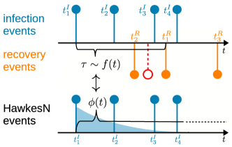
Figure 1. A sample stochastic SIR process including an infection event history until time $t$, i.e., $\operatorname{\mathcal{H}}^{C}_{t}=\{t^{I}_{1},...,t^{I}_{4}\}$, and recovery events $\{t^{R}_{2},t^{R}_{1},t^{R}_{3}\}$. Infected individuals recover at time intervals $\tau$ following a distribution $f(t)$. The bottom plot presents a corresponding realization of HawkesN events. HawkesN events generate descendants with the intensity rate $\phi(t)$. A connection between $f(t)$ and $\phi(t)$ is explored when $f(t)$ is assumed of arbitrary parametric forms. The red color marks an invalid recovery event given upcoming infections.

2. Preliminaries

In this section, we discuss two classes of stochastic event models, and highlight the missing link between them.

SIR models, originally proposed by Kermack and McKendrick (1927), describe the number of people infected by an epidemic in a fixed population over time. The name stands for the three possible states for individuals — those in a Susceptible state can get Infected, and those infected will eventually Recover or be Removed, and they are no longer prone to the infection. The stochastic variant of the SIR model (Bartlett, 1949) is concerned with individual state changes, rather than expected volumes of individuals in each state. The transition of individuals from susceptible to infected is described by the infection process, and that from infected to recovered by the recovery process.

One can represent the stochastic SIR in a fixed population of size $N$ as two sets of random event times, for the infections and recoveries, respectively. Let $\operatorname{\mathcal{H}}^{C}_{t}$ denote the set of infection event times that happened before time $t$, and $C_{t}=|\operatorname{\mathcal{H}}^{C}_{t}|$ is the number of infection events up to time $t$. Let $i$ index individuals in accordance with their infection time sequence, then $\operatorname{\mathcal{H}}^{C}_{t}=\{t_{i}^{I}\mid t_{1}^{I}=0,t_{1}^{I}<\ldots<t_{C_{t}}^{I}<t\}$. The short hand C stands for cumulative, i.e., $\operatorname{\mathcal{H}}^{C}_{t}$ and $C_{t}$ are not affected by the random events of individuals recovering. Similarly, let $\operatorname{\mathcal{H}}^{R}_{t}=\{t_{j}^{R}\mid 0<t_{j}^{R}<t,t_{j}^{R}>t_{j}^{I}\}$ denote a set of recovery event times before time $t$, and let $R_{t}=|\operatorname{\mathcal{H}}^{R}_{t}|$ be the number of individuals recovered by time $t$. We use $U()$ to denote the (index) set of individuals in an event history $\operatorname{\mathcal{H}}$. It follows from the sequential indexing that $U(\operatorname{\mathcal{H}}^{C}_{t})=\{1,2,\ldots,C_{t}\}$, and that the set of recovered individuals is a subset of those infected $U(\operatorname{\mathcal{H}}^{R}_{t})\subset U(\operatorname{\mathcal{H}}^{C}_{t})$. We use $\operatorname{\mathcal{H}}^{I}_{t}$ to express the set of infection event times of infected individuals who have not recovered by time $t$, i.e., $\operatorname{\mathcal{H}}^{I}_{t}=\{t^{I}_{j}\mid t^{I}_{j}<t,t^{R}_{j}>t\}$, and $I_{t}=|\operatorname{\mathcal{H}}^{I}_{t}|$. It is easy to see that the still infected set complements the recovered set $U(\operatorname{\mathcal{H}}^{C}_{t})=U(\operatorname{\mathcal{H}}^{R}_{t})\cup U(\operatorname{\mathcal{H}}^{I}_{t})$, and $C_{t}=R_{t}+I_{t}$. Fig. 1 shows an example of a stochastic SIR process. Based on the definitions above we have: $\operatorname{\mathcal{H}}^{C}_{t}=\{t^{I}_{1},t^{I}_{2},t^{I}_{3},t^{I}_{4}\}$, $\operatorname{\mathcal{H}}^{R}_{t}=\{t^{R}_{2},t^{R}_{1},t^{R}_{3}\}$, $\operatorname{\mathcal{H}}^{I}_{t}=\{t^{I}_{4}\}$, $C_{t}=4$, $R_{t}=3$, $I_{t}=1$, at time $t=t_{3}^{R}+\epsilon$. The susceptible individuals are the ones who have never been infected, namely are currently neither infected nor recovered: $S_{t}=~{}N-C_{t}=~{}N-I_{t}-R_{t}$.

The stochastic SIR process is defined by an infection event intensity function $\lambda^{I}(t)$ and a recovery event intensity function $\lambda^{R}(t)$ (Yan, 2008)

(1) $$\lambda^{I}(t)=\beta\frac{S_{t}}{N}I_{t};\,\,\,\,\lambda^{R}(t)=\gamma I_{t}$$

where $\beta$ and $\gamma$ are known as the infection rate and the recovery rate in SIR terminology. The total infection rate is proportional to the susceptible population $S_{t}$ and the infected population $I_{t}$. Each infected individual recovers independently with the same recovery rate $\gamma$, hence the total recovery rate is proportional to the size of the infected population. It is also assumed that the recovery process is simple (Daley and Vere-Jones, 2008), i.e., only one infection or recovery event can happen in any infinitesimal time interval.

Consider the random variable recovery time — the elapsed time between an individual’s infection and recovery. Eq. 1 implies that the recovery time is exponentially distributed $f(t)=\gamma e^{-\gamma t}$ (Yan, 2008).

Hawkes processes are a type of self-exciting point processes, i.e. processes in which the occurrence of events increases the likelihood of future events (Hawkes, 1971). This property is modeled via the intensity function:

(2) $$\lambda(t)=\mu+\sum_{t_{i}<t}\phi(t-t_{i})$$

where $\mu$ is the background intensity, and $\phi:\operatorname{\mathbb{R}}^{+}\rightarrow\operatorname{\mathbb{R}}^{+}$ is known as the triggering kernel — the rate of new events generated by event $t_{i}$ — and the summation aggregates the influences of all past events.

HawkesN process is a finite-population variant of the Hawkes process (Rizoiu et al., 2018b). Assuming the diffusion occurs in a fixed population of size $N$, the event intensity is modulated by the proportion of remaining population:

(3) $$\lambda^{H}(t)=\frac{N-N_{t}}{N}\sum_{t_{i}<t}\phi(t-t_{i})$$

$N_{t}$ is the number of events up to time $t$, the background intensity $\mu$ is set to zero and the first event happens at time $0$, i.e., $N_{0}=1$.

The stochastic SIR and Hawkes processes have been developed by separate scientific communities for modeling different natural phenomena (epidemics and financial transactions/earthquakes, respectively). It is desirable to connect these apparently disparate tools using the common language of stochastic point processes.

Table 1. Examples of HawkesN kernel functions $\phi(t)$, the corresponding SIR recovery time distributions $f(t)$ and hazard functions $h(t)$ following Eqs. (8)(9)(10). Parameter ranges: $\theta>1$ for Tsallis Q-Exponential kernel, $\kappa>0$, $\theta>0$, $c>0$ for all others.

HawkesN	HawkesN Kernel	SIR Recovery Time	SIR Recovery	Time
Kernel Name	Function $\displaystyle\phi(t)$	Distribution $\displaystyle f(t)$	Hazard $\displaystyle h(t)$	Constraint $t$
Linear	$\displaystyle-\kappa\theta t+\kappa$	$\displaystyle\theta$	$\displaystyle\frac{\theta}{-\theta t+1}$	$\displaystyle(0,\frac{\kappa}{\theta})$
Quadratic	$\displaystyle\kappa\frac{\theta^{2}}{4}t^{2}-\kappa\theta t+\kappa$	$\displaystyle-\frac{\theta^{2}}{2}t+\theta$	$\displaystyle\frac{\theta^{2}t-2\theta}{\theta^{2}t^{2}-4\theta t+4}$	$\displaystyle(0,\frac{2}{\theta})$
Gaussian	${\kappa e^{-\frac{t^{2}}{2\theta^{2}}}}$	$\displaystyle\frac{t}{\theta^{2}}e^{-\frac{t^{2}}{2\theta}}$	$\displaystyle\frac{1}{\theta^{2}}t$	$\displaystyle(0,\infty)$
Tsallis Q-Exponential (Lima and Choi, 2018)	$\displaystyle\kappa\left[1+(\theta-1)t\right]^{\frac{1}{1-\theta}}$	$\displaystyle\left[1+(\theta-1)t\right]^{\frac{\theta}{1-\theta}}$	$\displaystyle 1+(\theta-1)t$	$\displaystyle(0,\infty)$
Exponential (Hawkes, 1971)	$\displaystyle\kappa\theta e^{-\theta t}$	$\displaystyle\theta e^{-\theta t}$	$\displaystyle\theta$	$\displaystyle(0,\infty)$
Power-law (Mishra et al., 2016)	$\displaystyle\kappa(t+c)^{-(1+\theta)}$	$\displaystyle c^{1+\theta}(1+\theta)(t+c)^{-(2+\theta)}$	$\displaystyle\frac{1+\theta}{t+c}$	$\displaystyle(0,\infty)$

3. Linking SIR and HawkesN

First, we present a generalized stochastic SIR model with an arbitrary recovery time distribution, and next we reveal the connection between the general stochastic SIR and HawkesN. Finally, we extend the generalized SIR model with concepts from the Hawkes models.

3.1. SIR with general recovery distributions

As discussed in Section 2, the stochastic SIR process implicitly assumes that recovery times of infected individuals are exponentially distributed. Here we relax this assumption by letting recovery times follow an arbitrary distribution $f(t)$. The recovery intensity for each individual is given by the hazard function $h(t)$ (Cox and Oakes, 1984), i.e., the recovery time distribution conditioned on recovering after time $t$:

(4) $$h(t)=\frac{f(t)}{\int_{t}^{\infty}f(\tau)d\tau}$$

Considering that individuals recover independently, the overall recovery event intensity is the superposition of recovery intensities of the individuals still infected at time $t$:

(5) $$\lambda^{R}(t)=\sum_{t^{I}_{i}\in\operatorname{\mathcal{H}}^{I}_{t}}h(t-t^{I}_{i})=\sum_{t^{I}_{i}\in\operatorname{\mathcal{H}}^{I}_{t}}\frac{f(t-t^{I}_{i})}{\int_{t-t^{I}_{i}}^{\infty}f(\tau)d\tau}$$

The overall infection event intensity remains unchanged as in Eq. 1. Note that, when $f(t)$ is the exponential distribution, Eq. 5 simplifies to the infection intensity of the classic SIR in Eq. 1.

Despite being rather straightforward, to the best of our knowledge, this is the first work presenting this generalized SIR with arbitrary recovery distributions.

3.2. Marginalizing over recovery events

One of the challenges for using the SIR model for social media diffusions is that the definitions of infection and recovery are not straightforward. Infection events can be interpreted as posting, sharing or retweeting, and they are usually recorded in data traces; recovery events can be the times when these posts or discussion topics lose traction, which are rarely directly observable. This observation implies that one may treat recovery events as latent, and examine the expected process after marginalizing over them.

We use $\operatorname{\mathbb{E}}_{\{t^{R}_{i}\mid\operatorname{\mathcal{H}}^{C}_{t}\}}\left[\lambda^{I}(t)\right]$ to denote the expected infection intensity over all recovery event times up to time $t$:

$$\operatorname{\mathbb{E}}_{\{t^{R}_{i}\mid\operatorname{\mathcal{H}}^{C}_{t}\}}\left[\lambda^{I}(t)\right] \stackrel{{\scriptstyle\text{(a)}}}{{=}}\beta\frac{S_{t}}{N}\sum_{t^{I}_{i}\in\operatorname{\mathcal{H}}^{C}_{t}}\int^{\infty}_{t-t^{I}_{i}}f(\tau_{i}\mid\operatorname{\mathcal{H}}^{C}_{t})d\tau_{i}$$

(6) $$\stackrel{{\scriptstyle\text{(b)}}}{{\geq}}\beta\frac{S_{t}}{N}\sum_{t^{I}_{i}\in\operatorname{\mathcal{H}}^{C}_{t}}\int^{\infty}_{t-t^{I}_{i}}f(\tau_{i})d\tau_{i}$$

Eq. (6a) follows from  Rizoiu et al. (2018b). Step (b) is because, given $\operatorname{\mathcal{H}}^{C}_{t}$ an infection history observed up to time $t$, the recovery event time of the $i^{th}$ individual $t^{R}_{i}$ ($i\in U(\operatorname{\mathcal{H}}^{C}_{t})$) is dependent on the entire $\operatorname{\mathcal{H}}^{C}_{t}$. Fig. 1 illustrates this dependence with the red recovery event being an invalid candidate for $t^{R}_{1}$ given $\operatorname{\mathcal{H}}^{C}_{t}=\{t^{I}_{1},t^{I}_{2},t^{I}_{3},t^{I}_{4}\}$. Intuitively, if the first individual recovers at the time of the red event, there will be zero infected individuals afterwards, rendering impossible the rest of the diffusion. We simplify the dependence using the inequality in Eq. (6b) to the recovery time distribution $f(t)$. We show that

(7) $$\int^{\infty}_{t-t^{I}_{i}}f(\tau_{i}\mid\operatorname{\mathcal{H}}^{C}_{t})d\tau_{i}\geq\int^{\infty}_{t-t^{I}_{i}}f(\tau_{i})d\tau_{i}$$

with the left and right terms being equal when $t^{I}_{i}=\max\{\operatorname{\mathcal{H}}^{C}_{t}\}$. The proof is detailed in the online supplement (supplement, 2019, appendix A).

Comparing Eq. (6b) and Eq. 3, both $N-N_{t}$ (for HawkesN) and $S_{t}=N-C_{t}$ (for SIR) stand for the size of remaining susceptible population — hence the scaling factors $S_{t}/N$ and $(N-N_{t})/N$ are equivalent. Also, both Eq. (6b) and Eq. 3 sum over the infected population, and the integral in Eq. (6a) is a function of time since infection $t-t^{I}_{i}$. Therefore, marginalizing the recovery events reduces the infection intensity of the stochastic SIR to a lower bound — the HawkesN intensity — as long as the following relationship between the HawkeN kernel and recover time distribution holds:

(8) $$\phi(t)=\beta\int_{t}^{\infty}f(\tau)d\tau$$

We can express $f(t)$ in terms of $\phi(t)$. $f(t)$ is a probability density function which implies $f(t)\geq 0$ and $\int_{0}^{\infty}f(\tau)d\tau=1$, leading to $\phi(0)=\beta$:

(9) $$f(t) =-\frac{\phi^{\prime}(t)}{\phi(0)}$$

where we assume $\lim_{t\rightarrow\infty}f(t)=0$. Eq. 8 and Eq. 9 spell out the closed-form relationship between the recovery time distribution $f(t)$ of the stochastic SIR and the kernel function $\phi(t)$ of the HawkesN process. From Eq. 8, we note that this relationship only holds when $\phi(t)$ is a monotonically decreasing function. Incorporating Eq. 9 into Eq. 4, we can express the recovery hazard function in terms of the HawkesN kernel:

(10) $$h(t) =-\frac{\phi^{\prime}(t)}{\phi(t)}$$

Given that $\phi(t)$ is monotonically decreasing, $-\phi^{\prime}(t)$ and $h(t)$ are non-negative.

Table 1 lists six examples of HawkesN kernels, with their corresponding recovery time distributions and recovery hazard functions. The first three rows show the linear, quadratic, and Gaussian kernels, followed by the Tsallis Q-Exponential kernel used in quantum optics and atomic physics (Lima and Choi, 2018). The last two examples are the exponential kernel function and the power-law kernel function, widely used for financial data, geophysics, and information diffusion (Hawkes, 1971; Bacry et al., 2015; Mishra et al., 2016).

Relation to prior work. The relationship presented by Rizoiu et al. (2018b) omits the inequality shown in Eq. (6b), and it is a special case of the result in this work. Their reasoning is limited to the constant recovery hazard functions and the exponentially distributed recovery times, with $f(t)=\gamma e^{-\gamma t}$ and $\phi(t)=\kappa\theta e^{-\theta t}$. The main modeling contribution compared to (Rizoiu et al., 2018b; Yan, 2008) is a new set of analytical relationships among general recovery time distributions, kernel and hazard functions, in Eqs. (8)(9)(10).

3.3. Marked stochastic SIR

In real data and apart from event times, additional information about individual events is available, such as the user profile of a retweet event or patient characteristics in epidemics. Mathematically, the event history $\operatorname{\mathcal{H}}^{C}_{m}=\{(t^{I}_{1},m_{1}),...,(t^{I}_{n},m_{n})\}$ is a sequence of pairs of event times and extra event information also known as event marks. To leverage this information, marked variations of Hawkes process models are proposed to incorporate event marks as a scaling factor of kernel functions (Hawkes, 1971). This idea leads to a marked variation of the HawkesN model, with the intesity function as:

(11) $$\lambda^{H}_{m}(t)=\frac{N-N_{t}}{N}\sum_{(t^{I}_{i},m_{i})\in\operatorname{\mathcal{H}}^{I}_{m}(t)}m_{i}^{\rho}\phi(t-t^{I}_{i})$$

where $\rho$ controls a warping effect for the mark. Using the generalized connection introduced in Section 3.2, we are able to obtain a marked stochastic SIR model, whose infection intensity function is

(12) $$\lambda^{I}_{m}(t)=\beta\frac{S_{t}}{N}\sum_{(t^{I}_{i},m_{i})\in\operatorname{\mathcal{H}}^{I}_{m}(t)}m_{i}^{\rho}$$

where, comparing to Eq. 1, $I_{t}$ was decomposed to $\sum_{(t^{I}_{i},m_{i})\in\operatorname{\mathcal{H}}^{I}_{m}(t)}m_{i}^{\rho}$ to account for the individual mark information. The recovery intensity $\lambda_{m}^{R}(t)$ is identical to its unmarked counterpart in Eq. 5.

3.4. Branching factor for SIR

The basic reproduction number $R_{0}$ is an important quantity in epidemic models for determining whether an epidemic is likely to occur (Allen, 2008). This quantity conceptually connects to the branching factor $n^{*}$ from Hawkes processes which is defined as the expected number of events generated by a single infection event (Rizoiu et al., 2018b), i.e., $n^{*}=\int^{\infty}_{0}\phi(\tau)d\tau$. Building upon this observation and Eq. 8, we define $R_{0}$ for stochastic SIR with a general recovery time distribution as

(13) $$R_{0}=n^{*}=\beta\int^{\infty}_{0}\int^{\infty}_{\eta}f(\tau)d\tau d\eta$$

Based on (Newman, 2018), one can also generalize $R_{0}$ to $\beta\int^{\infty}_{0}\tau f(\tau)d\tau$, but we show in (supplement, 2019, appendix A) that this definition is equivalent to Eq. 13.

For marked variations, this quantity is computed by taking expectation over the distribution of event marks. Particularly, for retweet cascades where the event marks are the count of user followers, a power law distribution $P(m)=(\alpha-1)m^{-\alpha}$ of exponent $\alpha=2.016$ is determined by Mishra et al. (2016). We obtain

(14) $$R_{0}=n^{*}=\beta\frac{\alpha-1}{\alpha-1-\rho}\int^{\infty}_{0}\int^{\infty}_{\eta}f(\tau)d\tau d\eta$$

We refer to this quantity as just the branching factor $n^{*}$ in the following sections to avoid confusion.

Algorithm 1 Simulating generalized stochastic SIR

Input: Recovery time distribution $f(t)$, parameters $\{N,\beta\}$ Output: Infection event times $\operatorname{\mathcal{H}}^{C}$ and recovery event times $\operatorname{\mathcal{H}}^{R}$

1:  Set current time $T=0$.

2:  Initialize $\operatorname{\mathcal{H}}^{C}=\{0\}$ with one initial infection at time $0$.

3:  Initialize $\operatorname{\mathcal{H}}^{R}=\{\eta\}$ where $\eta\sim f(t)$ and $t^{R}_{1}=\eta$.

4:  while $|\operatorname{\mathcal{H}}^{C}|<N$ do

5:     $s=-\frac{log(u)}{\lambda*}$ where $u\sim U(0,1)$

6:     Compute $\Lambda^{I}(t)=\int^{t}_{0}\lambda^{I}(\eta)d\eta$ from $\operatorname{\mathcal{H}}^{C},\operatorname{\mathcal{H}}^{R}$

7:     $T=T+(\Lambda^{I})^{-1}(s)$

8:     if $T=\infty$ then

9:        break // No infection will occur

10:     else

11:        $\eta\sim f(t)$    // Draw recovery time, update histories

12:        $\operatorname{\mathcal{H}}^{R}=\operatorname{\mathcal{H}}^{R}\cup\{T+\eta\},\operatorname{\mathcal{H}}^{C}=\operatorname{\mathcal{H}}^{C}\cup\{T\}$

13:  return $\operatorname{\mathcal{H}}^{C},\operatorname{\mathcal{H}}^{R}$

4. A Set of Tools for Stochastic SIR

In this section, we introduce a set of tools for the stochastic SIR with general recovery time distributions and HawkesN, enabling one to simulate event realizations, estimate model parameters, assess fitted results and predict final diffusion sizes.

Generalized SIR simulation. The generalized SIR proposed in Eq. 5 cannot be simulated using the approach described by  Allen (2008) as the recovery event rate is no longer piece-wise constant. We show a procedure of sampling general stochastic SIR processes, by sampling each infection event and its corresponding recovery time.

Starting from the first infection event at $t=0$, Algorithm 1 iterates between two steps. Step one is to sample the recovery event time according to $f(t)$ (line 11-12), step two is to sample the next infection time by the random time change theorem (Laub et al., 2015) (line 5-7). Specifically, because future recovery times have been sampled for existing infection events, the infection event intensity can be then derived from Eq. 1 as a piece-wise constant function. The infection intensity leads to analytical forms of the cumulative infection intensity $\Lambda^{I}(t)=\int^{t}_{0}\lambda^{I}(s)ds$ and its inverse $(\Lambda^{I})^{-1}(\cdot)$. It is presented that $(\Lambda^{I})^{-1}(\cdot)$ can convert a time interval sampled from a Poisson process with unit rate (line 5) to an interval generated by the intensity function $\lambda^{I}(t)$ (line 7) (Laub et al., 2015). The process terminates when all $N$ individuals have been infected (line 4), or when the infection rate falls to zero (line 8).

Parameter estimation. We use maximum likelihood to estimate model parameters given event history via standard optimization packages. The likelihood functions of stochastic SIR and HawkesN can be derived from the general likelihoods for point processes (Daley and Vere-Jones, 2008). Details are in the online supplement (supplement, 2019, appendix B).

Suppose events are generated with an underlying stochastic SIR model. To estimate its parameters, when both infection and recovery events are observed, the stochastic SIR likelihood is maximized; when only infection events are observed, we estimate with the HawkesN likelihood to account for their latent recovery information. Due to the inequality in Eq. 6, the HawkesN likelihood is a biased estimator for stochastic SIR process parameters. We study this bias in Section 5.1 and we show empirically that it reduces as the branching factor increases.

Goodness-of-fit assessment. Given that the generalized SIR model can accommodate a wide range of recovery distribution functions, one natural question is how to assess the fitness of fitted models to observed events, choose between different parametric families and provide a guide to predict future events (Chen and Tan, 2018). Due to the aforementioned random time change theorem (Laub et al., 2015), for observed infection events $t^{I}_{i}\in\operatorname{\mathcal{H}}^{C}_{t}$ correctly described by an infection intensity function $\lambda^{I}(t)$, the cumulative infection intensities between infection events are time intervals generated from a Poisson process with unit rate or, equivalently, follow a unit rate exponential distribution:

(15) $$\mathcal{T}_{i}=\int^{t^{I}_{i}}_{t^{I}_{i-1}}\lambda^{I}(\tau)d\tau,\hskip 14.22636pt\mathcal{T}_{i}\sim e^{-t}$$

Three statistical tests are applied: the Kolmogorov-Smirnov (KS) test and the Excess Dispersion (ED) test to measure the significance of the proposition $\{\mathcal{T}_{i}\}\sim e^{-t}$; the Ljung-Box (LB) test to determine the independence among $\{\mathcal{T}_{i}\}$.

Lallouache and Challet (2016) note that the KS test is a more demanding test than the ED test. Specifically, the KS test evaluates the empirical cumulative density function (CDF) of $\{\mathcal{T}_{i}\}$ against the theoretical CDF of the unit rate exponential distribution (i.e., $1-e^{-t}$) producing two values: a p-value, indicating the significant level of $\{\mathcal{T}_{i}\}$ not being drawn from the nominated theoretical CDF, and a distance $D$ between the empirical CDF and the theoretical CDF (Massey Jr, 1951). As models presented in this paper are evaluated against the same theoretical CDF, we employ this distance measure $D$ as a fitting performance metric for model comparison.

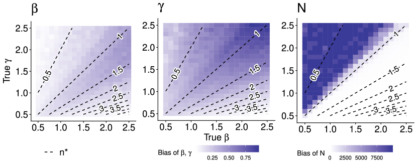
(a) Exponential

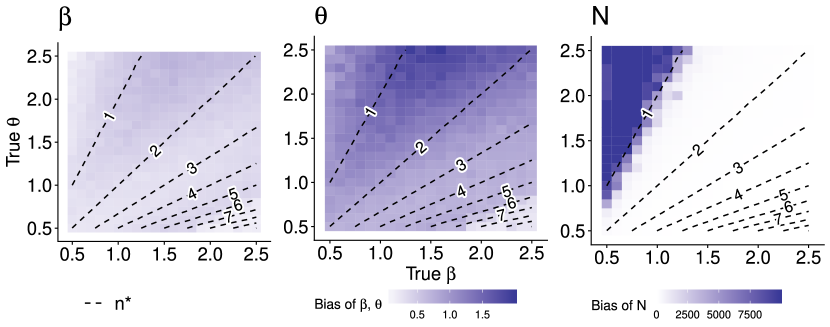
(b) Power-law

Figure 2. Bias of estimating parameters with HawkesN likelihood functions on simulated stochastic SIR infection events. Stochastic SIR with an exponential (a) and a power-law (b) recovery time distributions are evaluated. Chosen parameters are: (a) $N=200,\beta=\gamma=\{0.5,0.6,...,2.5\}$; (b) $N=200,c=2,\beta=\theta=\{0.5,0.6,...,2.5\}$. Estimation bias is computed with absolute errors — lighter colors indicate lower bias. The dotted contour lines are the branching factors given the parameter sets.

Diffusion final size prediction Point processes are generally applied for event history explanation and not optimized for prediction. To predict the diffusion final size (a.k.a the popularity for a Twitter cascade), we follow (Mishra et al., 2016) by using a regression layer on top of the proposed models. We predict a quantity $\sigma$ which can be interpreted as the proportion of remaining population that will be involved in the diffusion, i.e.,

(16) $$\hat{C}_{\infty}=C_{t}+\sigma(N-C_{t})$$

where $t$ is the observation time, $C_{t}$ is the number of cumulative infection events, $N$ is the fitted population size and $\hat{C}_{\infty}$ is the predicted diffusion final size. We note that $\sigma>1$ is possible due to the underestimation of $N$ given observed events or the growth of population as diffusion unfolds. We use the fitted parameters and the derived branching factor (e.g., $\{\beta,\gamma,\rho,N,n^{*}\}$ for exponentially recovered stochastic SIR) as features to train a $sigma$ predictor. This setup can also be applied to HawkesN given $N_{t}$ and its fitted parameters. The prediction experiment is set up to reproduce experiments in (Mishra et al., 2016), and we further detail it in Section 5.

5. Experiments

We first study the fitting of SIR parameters when the recovery times are not observed, and we design an empirical validation of the connection between the stochastic SIR and the HawkesN models through simulation and parameter estimation (in Section 5.1). Next, we investigate the performance of HawkesN models on three large Twitter cascade datasets in terms of goodness-of-fit, holdout log-likelihood and final diffusion size prediction (in Section 5.2).

Models and fitting. We use the following abbreviations when presenting our results: EXP, PL and QEXP, stand for Hawkes models with the exponential (Hawkes, 1971), power-law (Mishra et al., 2016) and Tsallis Q-Exponential kernel functions, respectively; EXPN, PLN and QEXPN, refer to HawkesN models with corresponding kernel functions; SI is the stochastic Suscepitable-Infected model as an epidemic model benchmark for comparison. The estimation of Hawkes models is performed as described by Mishra et al. (2016), i.e., the model parameters are fitted on an initial training part of a cascade through maximizing the log-likelihood functions. The log-likelihood functions can be found in the online supplement (supplement, 2019, appendix B) for HawkesN, and in (Mishra et al., 2016) for Hawkes. The parameter learning and simulation of the stochastic SI model can be adopted from the stochastic SIR model with $\gamma=0$.

5.1. Fitting SIR parameters with latent recoveries

In many applications, including in epidemiology, the recovery events are unobserved. It is therefore desirable to be able to fit the SIR model using infections events only. In this section we show how to achieve this, and we empirically validate the connection shown in LABEL:{sec:marginalizing} by simulating stochastic SIR and retrieving SIR parameters with the HawkesN log-likelihood functions with corresponding kernel functions. We construct a rich set of parameters for stochastic SIR with the exponential (Fig. 2a) and power-law (Fig. 2b) recovery time distributions. For each parameter set shown in Fig. 2 (each grid cell), we simulate $1000$ stochastic SIR realizations (using Algorithm 1). We hide the recovery events $\operatorname{\mathcal{H}}^{R}_{t}$ of these realizations and we fit HawkesN processes on infection event times $\operatorname{\mathcal{H}}^{C}_{t}$. We jointly fit $100$ realizations at a time by summing their log-likelihood functions.

In each grid cell in Fig. 2, the colors shows the fitting bias — i.e., the absolute error between simulation parameters and the median of fitted parameters. Note that, for ease of comparison, we have transformed the fitted HawkesN parameters into SIR parameters (using Eqs. 8 and 9, and Table 1). Also we notice in experiments that the power-law kernel as defined in (Mishra et al., 2016) is over-determined, and we fix $c=2$ both in simulation and in fitting.

Visibly, the bias of $\beta$ is relatively small due to its direct presence in the infection intensity function $\lambda^{I}(t)$. For the other parameters, their bias starts relatively high for low values of the branching factor (upper-left corners in Fig. 2, shown as contour lines) and gradually diminishes as the branching factor grows. When the branching factor is large (bottom-right corners in Fig. 2), the fitted parameters match closely with the simulation parameters. Processes with large branching factors are commonly of interest (e.g., $R_{0}=18$ for measles in epidemiology (Brauer, 2008)). For this reason, this evaluation supports the application of HawkesN log-likelihood functions to retrieve SIR parameters when recovery event times are missing and high branching factors are observed.

5.2. Modeling diffusions on Twitter

Table 2. Statistics of the three social media datasets.

	#cascades	#tweets	Min.	Mean	Median
ActiveRT	39,970	7,873,733	20	197	41
Seismic	166,076	34,784,488	50	209	111
NEWS	20,093	3,252,549	50	162	90

(a) EXPN vs. PL on NEWS

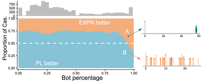
(b) EXPN vs. PL on ActiveRT w.r.t. percentage of bots in cascades

Figure 3. Comparing model goodness-of-fit using KS test values. (a) The most distinct model pair, EXPN and PL, on NEWS where colors of bins represent proportions of cascades that are better fitted by the model. Yellow means there is no cascade in the bins. (b) EXPN compares to PL on ActiveRT in terms of the percentage of bots involved in observed retweet cascades. The upper-panel histogram counts the number of cascades at different bot percentages; the lower-panel plot depicts proportions of cascades better fitted by EXPN or PL at given bot percentages. Two high bot-percetage cascade examples (cascade A and cascade B) better fitted by EXPN and PL, respectively, are shown on the right-hand side.

Datasets. We use three publicly available Twitter datasets containing retweet cascade — individual sequences of retweet events following a single initial tweet. Each tweet in the cascade is considered to be an infection event, i.e., a cascade is the collection $\operatorname{\mathcal{H}}^{C}=\{(t^{I}_{1},m_{1}),(t^{I}_{2},m_{2}),...\}$ where $t^{I}_{i}\in\operatorname{\mathcal{H}}^{C}$ is the time stamp of the $i^{th}$ retweet in the cascade and $m_{i}$ is its associated mark information, namely the number of followers of the user. The Seismic dataset was constructed by Zhao et al. (2015), and it contains a subset of all tweets in a month. The NEWS dataset was collected by Mishra et al. (2016) by crawling all tweets that contain links to popular news sites, such as New York Times and CNN, for four months in 2015. The ActiveRT dataset was collected by Rizoiu et al. (2017) over 6 months in 2014, by capturing all tweets containing links to Youtube videos. Table 2 summarizes the three datasets.

Table 3. Goodness-of-fit assessments on three datasets. Models are fitted on initial $40\%$ of each cascade event history with marks. The numbers in each cell indicate the percentages of cascades for which each model passes the nominated statistical tests (in Section 4) at the $0.01$ significance level. Darker colors signify a larger fraction of cascades passing.

	Test	EXP	EXPN	PL	PLN	QEXP	QEXPN	SI
ActiveRT	KS
	ED
	LB
Seismic	KS
	ED
	LB
NEWS	KS
	ED
	LB

Goodness-of-fit tests. We first conduct the goodness-of-fit tests described in Section 4 on all three datasets. The first $40\%$ of event history of each cascade is used for model fitting. Table 3 shows the percentages of cascades for which each model passes the tests at a $0.01$ significance level. We note that the passing rates of the SI model is consistantly worse than other models due to the model simplicity, so we focus our following experiments and discussions only on other models.

First, we see that the statistical test on the independence of transformed event times (LB test on $\{\mathcal{T}_{i}\}$ in Eq. 15) presents high passing percentages ($97.57\%\pm 1.16\%$) across all models (except SI) and datasets. The other two tests (KS test and ED test) mostly agree on the performance of models with respect to each other, despite KS being a more demanding test.

When comparing Hawkes and HawkesN, we observe an increase in performance for the Tsallis Q-Exponential kernel (from QEXP to QEXPN), and a decrease from PL to PLN. EXP and EXPN, on the other hand, share similar performance. This indicates that the effect of modulating the Hawkes intensity by a finite population for modeling retweet cascades is dependent on the choice of kernel.

Model goodness-of-fit comparison. By leveraging distances produced in the KS tests, we explore the modeling performance differences for every given dataset. Given two models $M_{1}$ and $M_{2}$ that pass KS test on a cascade $\operatorname{\mathcal{H}}^{C}_{t}$, we assume $M_{1}$ fits $\operatorname{\mathcal{H}}^{C}_{t}$ better if it has a lower KS test distance than $M_{2}$, denoted $D_{M_{1}}(\operatorname{\mathcal{H}}^{C}_{t})<D_{M_{2}}(\operatorname{\mathcal{H}}^{C}_{t})$. Next, we tabulate the cascades in each dataset against two dimensions: cascade duration (the time of the last event) and cascade size (number of events), both in percentiles. Fig. 3(a) compares the two models with the higher KS passing rate (EXPN and PL), on the NEWS dataset (refer to (supplement, 2019, appendix C) for other model pairs and datasets). Grid cells depict the proportions of cascades that are better fitted by one model or the other. Visibly, EXPN fits better cascades with larger diffusion sizes and shorter diffusion durations, whereas PL performs better on less popular cascades with longer durations. This indicates that PL and EXPN are two complementary models on NEWS, capturing different diffusion dynamics.

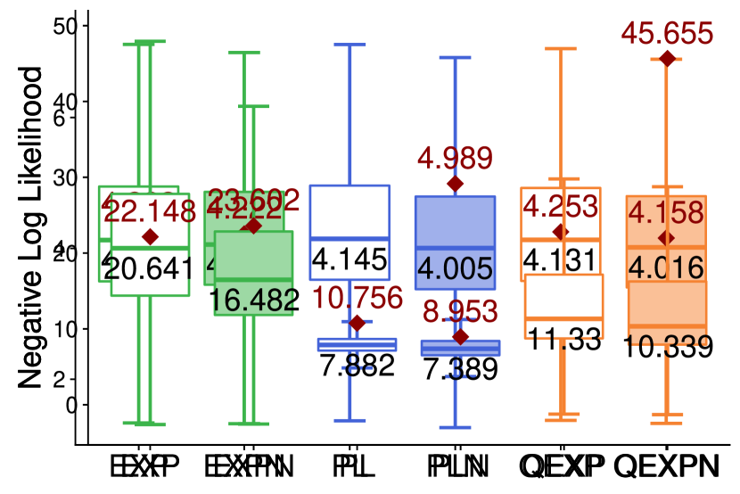
(a) Holdout log-likelihood

(b) Holdout log-likelihood with marks

(c) Popularity prediction performance

Figure 4. Fig. (a)-(b) depict holdout negative log-likelihood per event of six models on NEWS, with and without additional mark information. Fig. (c) shows diffusion final popularity prediction performance on NEWS. The red diamond shows the mean value in each boxplot — lower is better.

Linking modeling to botness. Here, we investigate a possible factor that induces the retweet dynamics that are better captured by EXPN compared to PL: non-human participation in cascades. We choose to analyze ActiveRT where the user information of individual events is available. We use the Botometer API (Yang et al., 2019) to identify Twitter bots and we collect data for $1,174,248$ unique users involved in the first $40\%$ event history of the $39,549$ cascades in ActiveRT. Due to the rate limit of the API, we only crawled cascades that have less than $2,500$ events. Given a user $i$, there are three possible outcomes from the API: a botness score $b_{i}\in[0,1]$ of the user; when the user has a private profile; or when the user was suspended by Twitter. As this data was collected $5$ years after the creation of ActiveRT in 2019, we assume users suspended by Twitter are bots. Eventually, we classify users who have been suspended or who have $b_{i}\geq 0.6$ as bots (Rizoiu et al., 2018a).

First, we group the cascades based on the proportion of bots that participate in each of them (in percentiles). For each percentile bin, Fig. 3(b) displays the proportions of cascades better fitted by EXPN and PL. We only keep cascades that satisfy $|D_{EXPN}(\cdot)-D_{PL}(\cdot)|\geq 0.05$ to identify the cascades significantly better fitted by each model. This condition filters out $72.96\%$ of cascades suggesting that EXPN and PL show similar performance on most cascades. We find that, while for most of the remaining cascades PL fits better than EXPN, when more than $90\%$ of bots involve in a cascade, around $60\%$ of the cascades are better fitted by EXPN. In Fig. 3(b), we denote A, the bot dominated cascades better fitted by EXPN, and B, those better fitted by PL, and we show one typical example from each. Cascades in A exhibit densely clustered events, with large intervals of no activity between them, whereas the cascades in B have the events more evenly spread. Intuitively, the temporal behavior of cascades in A tends to be more bot-driven, as bots retweet each other in rapid sequences and with small delays.

Generalization to unseen data. On each of the three dataset, we fit the parameters of all six models. We follow the experimental setup in (Rizoiu et al., 2018b): $40\%$ of the tweets in each cascade are used to fit model parameters, and we report the negative log-likelihood on the remaining $60\%$ of the events normalized by the event count.

Fig. 4a and b show as boxplots the generalization performance on NEWS, without and with marks respectively. Two conclusions emerge. First, the power-law kernel for both Hawkes and HawkesN consistently outperforms other kernel functions. This emphasizes the importance of developing the generalized SIR model, as different types of parametric kernel function might fit different types of data better. Second, HawkesN outperforms Hawkes confirming results reported in (Rizoiu et al., 2018b). The results on the other datasets depict a very similar conclusion, and they are shown in the online supplement (supplement, 2019, appendix C).

Popularity prediction. We predict final retweet cascade popularity following the setup described in  (Mishra et al., 2016). We observe each cascade for one hour and we fit model parameters; we predict final diffusion sizes (popularity) and test against the observed final cascade size. We measure performance using the Absolute Relative Error (ARE):

$$ARE=\frac{|\hat{N}_{\infty}-N_{\infty}|}{N_{\infty}}$$

where $\hat{N}_{\infty}$ and $N_{\infty}$ are the predicted size and the true size, respectively. We compare HawkesN models to the Hawkes models (EXP, PL), and to SEISMIC (Zhao et al., 2015). We use the GBM package in R (Greenwell et al., 2019) to train the $\sigma$ predictor described in Section 4. Furthermore, we adopt the observation that EXPN and PL are two complementary models on NEWS to introduce a combined model by averaging EXPN and PL prediction outcomes (Zhou, 2012). Results are reported with 10-fold cross validation where 6 folds are used for testing after trained on 4 folds during each iteration.

Fig. 4(c) shows the prediction performances on the NEWS. The performances on Seismic (also employed by Mishra et al. (2016), where it is called  TWEET-1MO) and on ActiveRT are shown in the online supplement (supplement, 2019, appendix C). Among all the Hawkes and HawkesN models, PL delivers the best prediction performance, and EXPN predicts better than EXP. These observations align with analyses in the previous sections. Overall, the combined model, EXPN+PL, consistently outperforms all other models, on all datasets. It provides a choice to deal with complementary modeling power of kernel functions on different cascades. This only reinforces the conclusion that there may exist more than one cascade dynamics, and that each model captures the best one of them.

6. Discussion and conclusion

In this work, we introduce a connection between generalized stochastic SIR models and self-exciting point processes in a finite population. The connection stems from the relationship between the recovery time distributions in SIR and the kernel functions in HawkesN processes. In addition, we develope algorithms for simulation, parameter estimation and evaluation for the stochastic SIR processes and the corresponding HawkesN processes. The modeling insights and the computational tools describe a rich set of self-exciting kernel functions, and they are more general than traditional stochastic SIR with piece-wise constant rates. In fact, it describes SIR with arbitrary recovery time distributions, and monotonically decreasing Hawkes kernels. We compare models with three kernel functions — an exponential, a power-law and a Tsallis Q-Exponential — on three large Twitter retweet cascade datasets. We observe differences in model performance in terms of goodness-of-fit tests. Final popularity prediction is improved by combining two complementary models.

Limitations and future work Non-monotonically decreasing kernel functions, such as the Rayleigh function, have been used in the point process literature (Ding et al., 2015; Mishra et al., 2016; Gomez-Rodriguez et al., 2011). Although it cannot be linked to the CCDF of recovery events in epidemics, the intuition of the Rayleigh function stems from the concept of the disease incubation period in epidemiology. We plan to broaden the connection, e.g., between HawkesN and variants in the epidemic models family.

In general, this newly established bridge between distinct classes of stochastic point processes opens up many research topics such as using modern machine learning tools to design objectives and estimation procedures, causal inference in epidemic models, and novel applications of either model in new data domains.

Software and Runtime Information

The simulation and fitting algorithms described in Section 3 have been implemented as an R package available on http://bit.ly/34qiDTK and the code for reproducing experiments in Section 5 can be found on https://bit.ly/3697ojK. Fitting HawkesN models on a $500$ event cascade takes $4.8$ minutes in average with $10$ parallel random parameter initializations on $2.2$GHz cpus where the likelihood function evaluation complexity is quadratic in the number of events.

Acknowledgments

This research is supported by Asian Office of Aerospace Research and Development (AOARD) Grant 19IOA08, Australian Research Council Discovery Project DP180101985 and the Data61, CSIRO PhD scholarship. We thank our reviewers, Swapnil Mishra and other lab members at ANU CMLab for their helpful comments. We also thank the National Computational Infrastructure (NCI) for providing computational resources, supported by the Australian Government.

Accompanying the submission Modeling Information Cascades with Self-exciting Processes via Generalized Epidemic Models.

Appendix A Linking SIR to Hawkes

A.1. Detailed derivation of the inequality between generalized stochastic SIR and HawkesN

We use $\operatorname{\mathbb{E}}_{\{t^{R}_{i}|\operatorname{\mathcal{H}}^{C}_{t}\}}\left[\lambda^{I}(t)\right]$ to denote the expected infection intensity over all recovery event times of infected individuals up to time $t$:

$$\operatorname{\mathbb{E}}_{\{t^{R}_{i}|\operatorname{\mathcal{H}}^{C}_{t}\}}\left[\lambda^{I}(t)\right]$$

$$\stackrel{{\scriptstyle\text{(a)}}}{{=}}\beta\frac{S_{t}}{N}\operatorname{\mathbb{E}}_{\{t^{R}_{i}|\operatorname{\mathcal{H}}^{C}_{t}\}}\left[I_{t}\right]$$

$$\stackrel{{\scriptstyle\text{(b)}}}{{=}}\beta\frac{S_{t}}{N}\operatorname{\mathbb{E}}_{\{t^{R}_{i}|\operatorname{\mathcal{H}}^{C}_{t}\}}\left[\sum_{t^{I}_{i}\in\operatorname{\mathcal{H}}^{C}_{t}}\mathds{1}(t^{R}_{i}-t^{I}_{i}>t-t^{I}_{i})\right]$$

$$\stackrel{{\scriptstyle\text{(c)}}}{{=}}\beta\frac{S_{t}}{N}\sum_{t^{I}_{i}\in\operatorname{\mathcal{H}}^{C}_{t}}\operatorname{\mathbb{E}}_{\{t^{R}_{i}|\operatorname{\mathcal{H}}^{C}_{t}\}}\left[\mathds{1}(t^{R}_{i}-t^{I}_{i}>t-t^{I}_{i})\right]$$

$$\stackrel{{\scriptstyle\text{(d)}}}{{=}}\beta\frac{S_{t}}{N}\sum_{t^{I}_{i}\in\operatorname{\mathcal{H}}^{C}_{t}}\int^{\infty}_{0}\mathds{1}(\tau_{i}>t-t^{I}_{i})f(\tau_{i}|\operatorname{\mathcal{H}}^{C}_{t})d\tau_{i}$$

$$\stackrel{{\scriptstyle\text{(e)}}}{{=}}\beta\frac{S_{t}}{N}\sum_{t^{I}_{i}\in\operatorname{\mathcal{H}}^{C}_{t}}\int^{\infty}_{t-t^{I}_{i}}f(\tau_{i}|\operatorname{\mathcal{H}}^{C}_{t})d\tau_{i}$$

(17) $$\stackrel{{\scriptstyle\text{(f)}}}{{\geq}}\beta\frac{S_{t}}{N}\sum_{t^{I}_{i}\in\operatorname{\mathcal{H}}^{C}_{t}}\int^{\infty}_{t-t^{I}_{i}}f(\tau_{i})d\tau_{i}$$

Here Eq. (17a) is due to the independence between $S_{t}$ and $t^{R}_{i}$ given $\operatorname{\mathcal{H}}^{C}_{t}$. Eq. (17b) follows from decomposing the step-wise stochastic process $I_{t}$ — that the recovery time of each individual therein is greater than time $t$, i.e., $t_{i}^{R}>t$. By definition $t_{i}^{R}>t_{i}^{I}$, we can subtract infection times $t_{i}^{I}$ on both sides and preserve the sign of the inequality — leading to $t_{i}^{R}-t_{i}^{I}>t-t_{i}^{I}$, which is easier to model since the left hand side correspond to the recovery time of the $i$-th infection. $\mathds{1}(x)$ is an indicator function that takes value $1$ if the proposition $x$ is true, $0$ otherwise. Eq. (17c) pushes the expectation into the summation due to known infection events. Eq. (17d) expands the expectation for each recovery time, and uses $\tau_{i}=t^{R}_{i}-t^{I}_{i}\sim f(\tau_{i}|\operatorname{\mathcal{H}}^{C}_{t})$ where the $i^{th}$ individual’s recovery time distribution is conditional. Eq. (17e) uses the definition of the indicator function to change the lower bound of integration.

To show the inequality in Eq. (17f), we reduce it down to proofing

(18) $$\int^{\infty}_{t-t^{I}_{i}}f(\tau_{i}|\operatorname{\mathcal{H}}^{C}_{t})d\tau_{i}\geq\int^{\infty}_{t-t^{I}_{i}}f(\tau_{i})d\tau_{i}\Longrightarrow\int^{t-t^{I}_{i}}_{0}f(\tau_{i}|\operatorname{\mathcal{H}}^{C}_{t})d\tau_{i}\leq\int^{t-t^{I}_{i}}_{0}f(\tau_{i})d\tau_{i}$$

which is equivalent to $\operatorname{\mathbb{P}}\left[t^{R}_{i}<t|\operatorname{\mathcal{H}}^{C}_{t}\right]\leq\operatorname{\mathbb{P}}\left[t^{R}_{i}<t\right]$. To proof this, we reason it from the perspective of a branching structure, namely any future event is a descendent event triggered by past event. We denote the infection events triggered by $i^{th}$ individual as $\operatorname{\mathcal{H}}^{C}_{i}=\{t^{I}_{j}|t^{I}_{j}\in\operatorname{\mathcal{H}}^{C}_{t},t^{I}_{i}<t^{I}_{j}<t\}$ and use $t^{I}_{m}=\max\{\operatorname{\mathcal{H}}^{C}_{i}\}$. Then we can see that $\operatorname{\mathbb{P}}\left[t^{R}_{i}<t|\operatorname{\mathcal{H}}^{C}_{t}\right]=\operatorname{\mathbb{P}}\left[t^{R}_{i}<t|\operatorname{\mathcal{H}}^{C}_{i}\right]$. Two possible cases emerge

• $\operatorname{\mathcal{H}}^{C}_{i}=\emptyset$: we have $\operatorname{\mathbb{P}}\left[t^{R}_{i}<t|\operatorname{\mathcal{H}}^{C}_{i}\right]=\operatorname{\mathbb{P}}\left[t^{R}_{i}<t\right]$ where the equality holds.

• $|\operatorname{\mathcal{H}}^{C}_{i}|>0$: we can also reduce the dependency with $\operatorname{\mathbb{P}}\left[t^{R}_{i}<t|\operatorname{\mathcal{H}}^{C}_{i}\right]=\operatorname{\mathbb{P}}\left[t^{I}_{m}<t^{R}_{i}<t\right]$. We then compare $\operatorname{\mathbb{P}}\left[t^{I}_{m}<t^{R}_{i}<t\right]=\int_{t^{I}_{m}-t^{I}_{i}}^{t-t^{I}_{i}}f(\tau)d\tau$ against $\operatorname{\mathbb{P}}\left[t^{R}_{i}<t\right]=\int_{0}^{t-t^{I}_{i}}f(\tau)\tau$ given recovery time distribution $f(t)$. As $f(t)\geq 0,\forall t\in R$, we conclude $\int_{0}^{t-t^{I}_{i}}f(\tau)\tau>\int_{t^{I}_{m}-t^{I}_{i}}^{t-t^{I}_{i}}f(\tau)d\tau$

Overall, that proofs $\int^{\infty}_{t-t^{I}_{i}}f(\tau_{i}|\operatorname{\mathcal{H}}^{C}_{t})d\tau_{i}\geq\int^{\infty}_{t-t^{I}_{i}}f(\tau_{i})d\tau_{i}$.

A.2. Emprical analysis of the intensity difference

In this section, we explore the difference between the expected infection intensity values of generalized stochastic SIR and the corresponding HawkesN intensity. Fig. 5(a) presents an example of this intensity difference given a specific parameter set. For a given stochastic SIR process, we approximate its expected infection intensity by fixing the infection events and simulating recovery events via standard rejection-sampling technique Daley2008. HawkesN intensity values, on the other hand, can be computed from Eq. 3. Fig. 5(b) explores the relative intensity difference between the two at various parameter combinations.

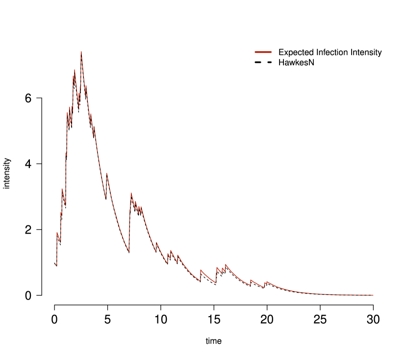
(a) Intensity difference between the expected infection intensity and HawkesN intensity (an exponential recovery time distribution: $N=50,\beta=1,\gamma=0.5$). The expected infection intensity is approximated with $2000$ simulations.

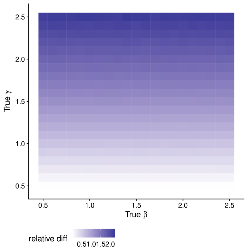
(b) Given the infection events in (a), the relative difference between the expected infection intensity values and the HawkesN intensity values given various parameters.

Figure 5.

A.3. Branching factor

For the classic SIR, the reproduction number $R_{0}$ is defined as newman2018networks

(19) $$R_{0}=\int^{\infty}_{0}\beta\tau\gamma e^{-\gamma\tau}d\tau$$

where $\beta\tau$ is the expected number of individuals contacted by an infected individual and integrating it with the recovery time distribution leads to $R_{0}$. We can then express it with a general recovery time distribution as $R_{0}=\int^{\infty}_{0}\beta\tau f(\tau)d\tau$. We show its equivalence to Eq. 13 as following

$$R_{0} =\int^{\infty}_{0}\beta\tau f(\tau)d\tau$$

(Integration by parts) $$=\beta\left[\tau\int^{\tau}_{0}f(\eta)d\eta\right]^{\infty}_{0}-\beta\int^{\infty}_{0}\int^{\tau}_{0}f(\eta)d\eta d\tau$$

(due to $$\int^{\infty}_{0}f(\eta)d\eta=1 =\beta\left[\tau\int^{\tau}_{0}f(\eta)d\eta\right]^{\infty}_{0}-\beta\int^{\infty}_{0}(1-\int^{\infty}_{\tau}f(\eta))d\eta d\tau$$)

$$=\beta\left[\tau\int^{\tau}_{0}f(\eta)d\eta\right]^{\infty}_{0}-\beta\left[\tau\right]^{\infty}_{0}+\beta\int^{\infty}_{0}\int^{\infty}_{\tau}f(\eta)d\eta d\tau$$

(due to $$\int^{0}_{0}f(\eta)d\eta=0 =\beta\left[\tau\int^{\tau}_{0}f(\eta)d\eta\right]_{\tau=\infty}-\beta\left[\tau\right]_{\tau=\infty}+\beta\int^{\infty}_{0}\int^{\infty}_{\tau}f(\eta)d\eta d\tau$$)

(due to $$\int^{\infty}_{0}f(\eta)d\eta=1 =\beta\int^{\infty}_{0}\int^{\infty}_{\tau}f(\eta)d\eta d\tau$$)

Appendix B Likelihood and Parameter Estimation

We conduct maximum likelihood estimation for parameter inference. For total population size $N$, we adopt the practice from both jin2013epidemiological and Rizoiu2017c: fitting $N$ as an unknown parameter. Let $\Theta^{E}$ denote the set of all parameters in the stochastic SIR models, e.g., $\Theta^{E}=\{\beta,\gamma,N\}$ for stochastic SIR described in Section 2. To estimate $\Theta^{E}$ from a given stochastic SIR process until time $t$ ($\operatorname{\mathcal{H}}^{C}_{t},\operatorname{\mathcal{H}}^{R}_{t}$) with a recovery time distribution $f(t)$, the likelihood function of $\Theta^{E}$ can be expressed based on the log-likelihood estimator for point processes Daley2008 as

(20) $$\mathcal{L}(\Theta^{E};\operatorname{\mathcal{H}}^{C}_{t},\operatorname{\mathcal{H}}^{R}_{t})= \sum_{t^{I}_{i}\in\operatorname{\mathcal{H}}^{C}_{t}}\log\lambda^{I}(t^{I}_{i})-\int_{0}^{t}\lambda^{I}(\tau)d\tau+\sum_{i\in U(\operatorname{\mathcal{H}}^{R}_{t})}\log f(t^{R}_{i}-t^{I}_{i})$$

The first two terms of RHS of Eq. 20 comes from

(21) $$\mathcal{L}(\Theta^{E};\operatorname{\mathcal{H}}^{C}_{t},\operatorname{\mathcal{H}}^{R}_{t}) =\log\prod_{t^{I}_{i}\in\operatorname{\mathcal{H}}^{C}_{t}}\lambda^{I}(t^{I}_{i})e^{-\int_{0}^{t^{I}_{i}}\lambda^{I}(u)du}=\log\prod_{t^{I}_{i}\in\operatorname{\mathcal{H}}^{C}_{t}}\lambda^{I}(t^{I}_{i})e^{-\int_{t^{I}_{i-1}}^{t^{I}_{i}}\lambda^{I}(u)du}$$

(22) $$=\log e^{-\int_{0}^{max\{\operatorname{\mathcal{H}}^{C}_{t}\}}\lambda^{I}(u)du}\prod_{t^{I}_{i}\in\operatorname{\mathcal{H}}^{C}_{t}}\lambda^{I}(t^{I}_{i})$$

(23) $$=-\int_{0}^{t}\lambda^{I}(\tau)d\tau+\sum_{t^{I}_{i}\in\operatorname{\mathcal{H}}^{C}_{t}}\log\lambda^{I}(t^{I}_{i})$$

When recovery events are not observed, i.e., only $\operatorname{\mathcal{H}}^{C}$ is presented, we take expectation over the recovery event history $\operatorname{\mathcal{H}}^{R}$ on Eq. 20: HawkesN log-likelihood functions after the solving integral part in Eq. 21 with different kernel functions are listed as following:

• Exponential

  $$\mathcal{L}_{EXP}(\Theta^{H};\operatorname{\mathcal{H}}^{C})=\sum_{j=2}^{n}\log\left(\lambda^{H}\left(t_{j}^{-}\right)\right)-\kappa\sum_{j=1}^{n-1}\sum_{l=j}^{n-1}\frac{N-l}{N}\left[e^{-\theta(t_{l}-t_{j})}-e^{-\theta(t_{l+1}-t_{j})}\right]$$

• Power-law

  $$\mathcal{L}_{PL}(\Theta^{H};\operatorname{\mathcal{H}}^{C})= \sum_{t_{i}\in\operatorname{\mathcal{H}}^{C}}\log\frac{N-i}{N}\kappa\sum_{t_{j}\in\operatorname{\mathcal{H}}^{C},t_{j}<t_{i}}(t_{i}-t_{j}+c)^{-(1+\theta)}$$

  $$-\kappa\theta\sum_{t_{i}\in\operatorname{\mathcal{H}}^{C},t_{i}<t_{n}}\sum_{t_{j}\in\operatorname{\mathcal{H}}^{C},t_{i}\leq t_{j}<t_{n}}\frac{N-j}{N}\left[(t_{j}-t_{i}+c)^{-\theta}-(t_{j+1}-t_{i}+c)^{-\theta}\right]$$

• Tsallis Q-EXP

  $$\mathcal{L}_{Q-EXP}(\Theta^{H};\operatorname{\mathcal{H}}^{C})= \sum_{t_{i}\in\operatorname{\mathcal{H}}^{C}}\log\frac{N-i}{N}\kappa\sum_{t_{j}\in\operatorname{\mathcal{H}}^{C},t_{j}<t_{i}}\left[1+(\theta-1)(t_{i}-t_{j})\right]^{\frac{1}{1-\theta}}$$

  $$-\frac{\kappa}{2-\theta}\sum_{t_{i}\in\operatorname{\mathcal{H}}^{C},t_{i}<t_{n}}\sum_{t_{j}\in\operatorname{\mathcal{H}}^{C},t_{i}\leq t_{j}<t_{n}}\frac{N-j}{N}\left[\left[1+(\theta-1)(t_{j}-t_{i})\right]^{\frac{2-\theta}{1-\theta}}-\left[1+(\theta-1)(t_{j+1}-t_{i})\right]^{\frac{2-\theta}{1-\theta}}\right]$$

Some natural constraints are applied on $N\geq C_{t}$ and on other parameters as in Table 1. Eqs. (20) (21) are non-linear functions and we use an optimization tool AMPL fourer1987ampl bridged with a non-linear solver Ipopt Wachter2006 for maximizing them and estimating model parameters.

After obtaining $\Theta^{H}$, Eq. 9 leads us to corresponding stochastic SIR parameters $\Theta^{E}$. Similarly, Eq. 8 links $\Theta^{E}$ inferred by Eq. 20 to $\Theta^{H}$. This helps one reveal the underlying recovery processes when missing recovery event data or concentrate on infection process yet leveraging both infection and recovery events in data.

Appendix C Extra experiment results

Fig. 6 presents the comparison of a most distinct model pair on each dataset. Fig. 7 shows the holdout log-likelihood values and popularity prediction performance of models fitted with event marks on all three retweet cascade datasets.

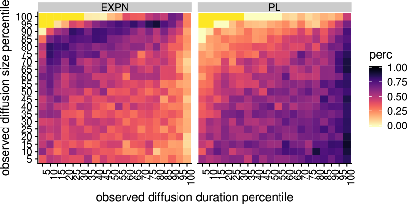
(a) NEWS: EXPN vs. PL

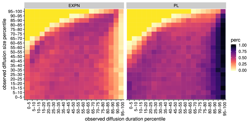
(b) Seismic: EXPN vs. PL

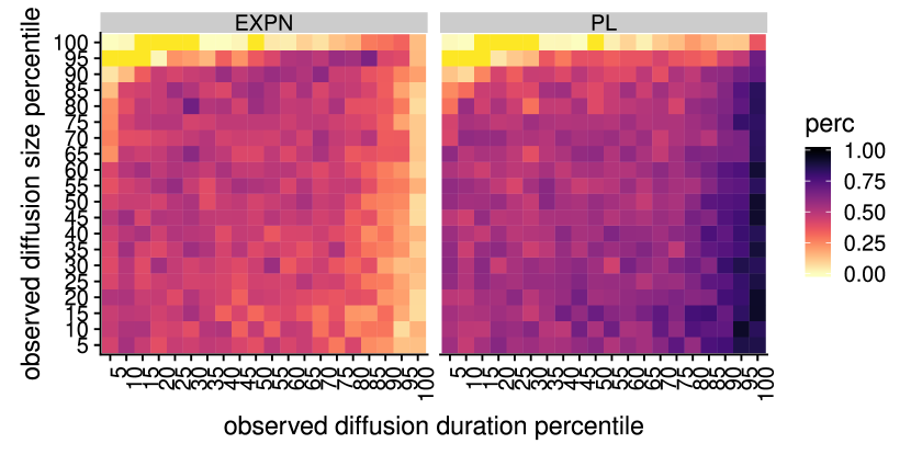
(c) ActiveRT: EXPN vs. PL

Figure 6.

(a) NEWS

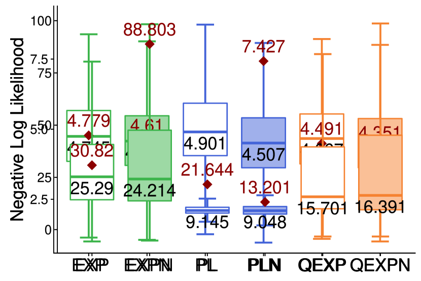
(b) ActiveRT

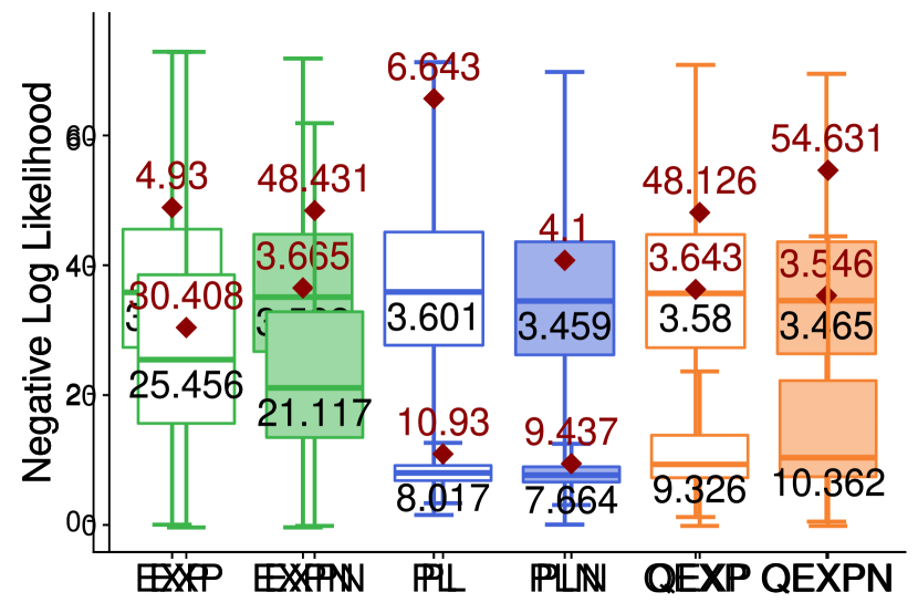
(c) Seismic

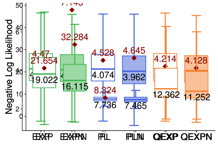
(d) NEWS with marks

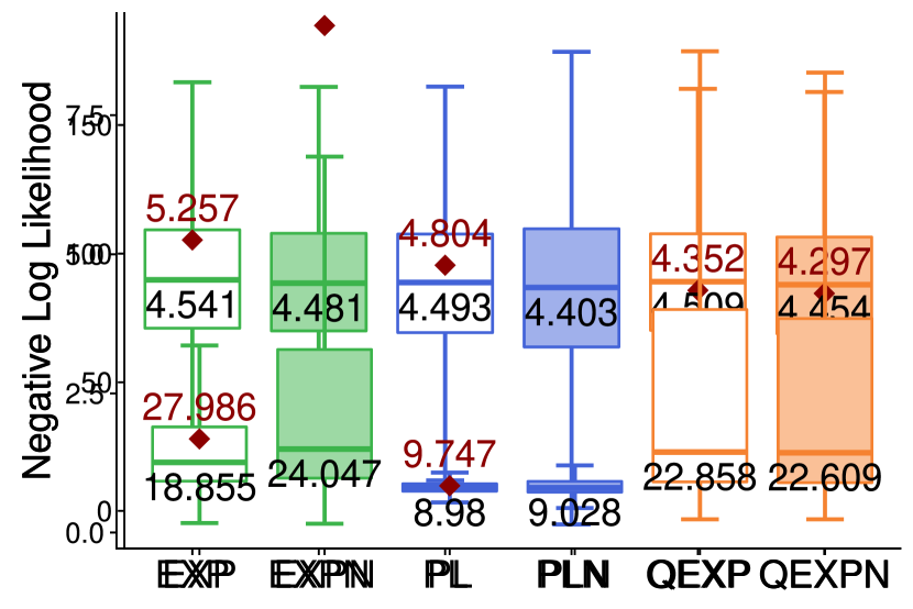
(e) ActiveRT with marks

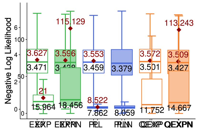
(f) Seismic with marks

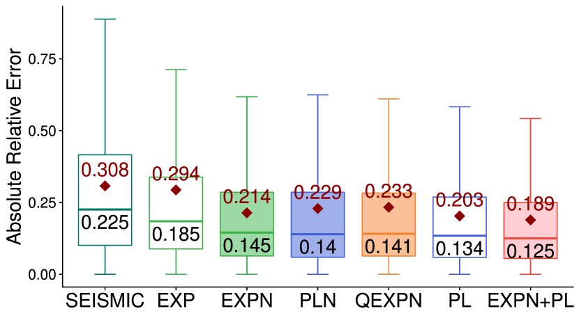
(g) Popularity prediction on News

(h) Popularity prediction on ActiveRT

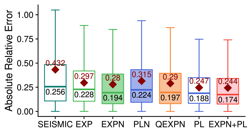
(i) Popularity prediction on Seismic

Figure 7. Fig. (a)-(f) are holdout negative log-likelihood of models on three datasets. Fig. (g)-(i) are popularity prediction performance on three datasets

Appendix D Compare size distributions of stochastic SIR and HawkesN

In this section, we empirically show the difference of stochastic SIR and HawkesN in terms of their process final size distributions given same set of parameters. We approximate their final size distributions (empirical cumulative density functions) via simulation with $1000$ simulated processes for each model and parameter set. Fig. 8 shows the results given different sets of parameters. From this plot, we notice that stochastic SIR processes consistently present higher probabilities of smaller cascade sizes and HawkesN models tend to generate larger size cascades for high branching factors.

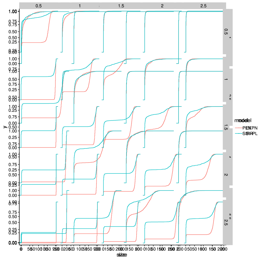
(a) EXPN vs stochastic SIR with an exponential recovery distribution

(b) PLN vs stochastic SIR with a power-law recovery distribution

Figure 8. Size distribution comparison between HawkesN models and stochastic SIR processes. The x axis and y axis are different parameter values ($\beta,\gamma$ for (a) and $c,\theta$ for (b), respectively). For each small plot, the x axises are the cascade sizes while the y axises are the corresponding empirical cumulative densities.

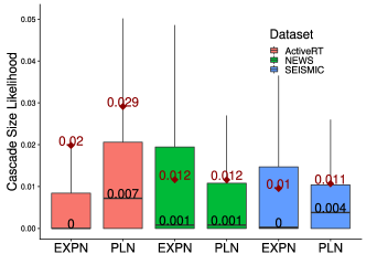
Figure 9. The likelihood of observed cascade sizes on ActiveRT, NEWS and Seismic, using EXPN and PLN. The parameters of each model are fitted using $40\%$ of the events in each cascade. The distributions of cascade size are approximated using 5000 simulations for each set of parameters — higher is better.

Appendix E Likelihood of cascade sizes.

We study the probability distribution of final size for Twitter cascades. Rizoiu2017c have proposed a Markov chain method to estimate the distribution of final cascade size, based on SIR’s memory-less property. However, stochastic SIR with non-exponentially distributed recovery times do not have this property. To overcome this problem, we employ a simulation-based computation of the size distribution. Given a parameter set $\Theta^{E}$ — the parameters of HawkesN fitted on $k$ events — we approximate the size distributions $\operatorname{\mathbb{P}}\left[|\operatorname{\mathcal{H}}^{C}|=j\middle|\Theta^{E},j\geq k\right]$ by converting the HawkesN parameters to stochastic SIR parameters, and applying Algorithm 1 to simulate $5000$ realizations for each cascade. We construct the empirical size distribution by aggregating the sizes of the realizations and smoothing the obtained distribution. Given $n$ the observed final size of a cascade, its likelihood under the constructed distribution is $\operatorname{\mathbb{P}}\left[|\operatorname{\mathcal{H}}^{C}|=n\middle|\Theta^{E}\right]$.

We employ the above methodology to compute the likelihood of the observed final size for three samples — one for each dataset — each sample containing $1000$ cascades. For every cascade we construct two size distributions, using HawkesN with an exponential and a power-law kernel respectively. Figure 9 aggregates the computed likelihoods, per dataset and per HawkesN kernel type. Each boxplot contains $1000$ datapoints. We observe that for ActiveRT and for Seismic, the observed final size is more likely under the distribution constructed using power-law kernel than under the exponential kernel. This is likely due to power-law kernel being long-tailed, and able to explain the minority of very large cascades occurring naturally Goel2015. For NEWS, the similar performances of the two kernels are likely due to news being time-sensitive content, and on average having smaller cascades.

ACM-Reference-Format acm

References

- (1)
- Allen (2008) Linda J. S. Allen. 2008. An Introduction to Stochastic Epidemic Models. In Mathematical Epidemiology. Springer, Chapter 3.
- Bacry et al. (2015) Emmanuel Bacry, Iacopo Mastromatteo, and Jean-François Muzy. 2015. Hawkes processes in finance. Market Microstructure and Liquidity (2015).
- Bartlett (1949) MS Bartlett. 1949. Some evolutionary stochastic processes. Journal of the Royal Statistical Society. Series B (Methodological) (1949).
- Brauer (2008) Fred Brauer. 2008. An Introduction to Stochastic Epidemic Models. In Mathematical Epidemiology. Springer, Chapter 2.
- Chen and Tan (2018) Feng Chen and Wai Hong Tan. 2018. Marked self-exciting point process modelling of information diffusion on Twitter. The Annals of Applied Statistics (2018).
- Cox and Oakes (1984) D. R. Cox and D Oakes. 1984. Analysis of survival data. Routledge.
- Daley and Vere-Jones (2008) Daryl J Daley and David Vere-Jones. 2008. Conditional Intensities and Likelihoods. In An introduction to the theory of point processes. Vol. I. Springer, Chapter 7.2.
- Ding et al. (2015) Wanying Ding, Yue Shang, Lifan Guo, Xiaohua Hu, Rui Yan, and Tingting He. 2015. Video popularity prediction by sentiment propagation via implicit network. In CIKM.
- Du et al. (2016) Nan Du, Hanjun Dai, Rakshit Trivedi, Utkarsh Upadhyay, Manuel Gomez-Rodriguez, and Le Song. 2016. Recurrent marked temporal point processes: Embedding event history to vector. In KDD. ACM.
- Gomez-Rodriguez et al. (2011) Manuel Gomez-Rodriguez, David Balduzzi, and Bernhard Schölkopf. 2011. Uncovering the temporal dynamics of diffusion networks. (2011).
- Greenwell et al. (2019) Brandon Greenwell, Bradley Boehmke, Jay Cunningham, and GBM Developers. 2019. gbm: Generalized Boosted Regression Models. R package version 2.1.5.
- Hawkes (1971) Alan G Hawkes. 1971. Spectra of some self-exciting and mutually exciting point processes. Biometrika (1971).
- Jin et al. (2013) Fang Jin, Edward Dougherty, Parang Saraf, Yang Cao, and Naren Ramakrishnan. 2013. Epidemiological modeling of news and rumors on twitter. In SNA-KDD Workshop. ACM.
- Jing and Smola (2017) How Jing and Alexander J Smola. 2017. Neural survival recommender. In WSDM.
- Johnson (1996) Don H Johnson. 1996. Point process models of single-neuron discharges. Journal of computational neuroscience (1996).
- Keeling and Grenfell (1997) Matthew J Keeling and BT Grenfell. 1997. Disease extinction and community size: modeling the persistence of measles. Science (1997).
- Kermack and McKendrick (1927) William Ogilvy Kermack and Anderson G McKendrick. 1927. A contribution to the mathematical theory of epidemics. Proceedings of the Royal Society of London. Series A, Containing Papers of a Mathematical and Physical Character (1927).
- Kimura et al. (2009) Masahiro Kimura, Kazumi Saito, and Hiroshi Motoda. 2009. Efficient Estimation of Influence Functions for SIS Model on Social Networks.. In IJCAI.