Robust Incremental State Estimation through Covariance Adaptation

Abstract

Recent advances in the fields of robotics and automation have spurred significant interest in robust state estimation. To enable robust state estimation, several methodologies have been proposed. One such technique, which has shown promising performance, is the concept of iteratively estimating a Gaussian Mixture Model (GMM), based upon the state estimation residuals, to characterize the measurement uncertainty model. Through this iterative process, the measurement uncertainty model is more accurately characterized, which enables robust state estimation through the appropriate de-weighting of erroneous observations. This approach, however, has traditionally required a batch estimation framework to enable the estimation of the measurement uncertainty model, which is not advantageous to robotic applications. In this paper, we propose an efficient, incremental extension to the measurement uncertainty model estimation paradigm. The incremental covariance estimation (ICE) approach, as detailed within this paper, is evaluated on several collected data sets, where it is shown to provide a significant increase in localization accuracy when compared to other state-of-the-art robust, incremental estimation algorithms.

I Introduction

The ability to infer information about the system and the operating environment is one of the key components enabling many robotic applications. To equip robotic platforms with this capability, several state estimation frameworks [1] have been developed (e.g., the Kalman filter [2], or the particle filter [3]).

The traditional state estimation methodologies perform efficiently and accurately when the collected observations adhere to the a priori models. However, in many robotic applications of interest, the observations can be degraded (e.g., global navigation satellite system (GNSS) observations in an urban environment, or RGB observations in a low-light setting), which cause a deviation between the collected observations and the assumed models. When this deviation is present, the traditional state estimation schemes (i.e., estimators that utilize the $l^{2}\text{-norm}$ exclusively to construct the cost-function) can breakdown [4].

To overcome the breakdown of traditional state estimators in data degraded scenarios, several robust estimation schemes have been developed. These robust estimation schemes reduce the effect that erroneous observations have on the estimation process by scaling the associated covariance matrix [5]. To enable this covariance scaling in practice, several implementations have been developed (i.e., maximum likelihood type estimators [6], switchable constraints [7], and dynamic covariance scaling (DCS) [8]).

To extend robust state estimation from the traditional uni-modal uncertainty model paradigm to a multi-modal implementation, the max-mixtures (MM) [9] approach was developed. The MM approach mitigates increased computation complexity generally assumed to accompany the incorporation of multi-modal uncertainty models by first assuming that the uncertainty model can be represented by a Gaussian mixture model (GMM), then selecting the single Gaussian component from the GMM that maximizes the likelihood of the individual observation given the current state estimate.

This MM approach was extended in [5] to enable the iterative estimation of the GMM, based upon the state estimation residuals, to characterize the measurement uncertainty model. Through this iterative process, the measurement uncertainty model is more accurately characterized, which enables robust state estimation through the appropriate de-weighting of erroneous observations. This approach, however, has traditionally required a batch [5], or fixed-lag [10] estimation framework to enable the estimation of the measurement uncertainty model, which is not advantageous to most robotic applications, as incremental updates are usually required. Additionally, as we’ll discuss in this paper, theses approaches are inefficient – both respect to memory and computation – in the estimation of the measurement uncertainty model.

Within this paper, we propose a novel extension to the measurement uncertainty model estimation paradigm. Specifically, we propose an efficient, incremental extension of the methodology. The efficiency of the approach is granted by incrementally adapting the uncertainty model with only a small subset of informative state estimation residuals (i.e., the state estimation residuals which do not adhere to the a priori model). The incremental nature of the approach is granted through recent advances within the probabilistics graphical model community (i.e., through the utilization of the incremental smoothing and mapping (iSAM2) [11] algorithm), in conjunction with the ability to merge GMM’s [12].

To provide a discussion of the proposed incremental covariance estimation (ICE) approach, the remainder of the paper is accordingly organized. First, a brief introduction to state estimation is provided in Section II, with a specific emphasis being placed on the current limitations of robust state estimation. Based upon the discussion provided in Section II, the discussion turns to the proposed ICE robust framework in Section III. In Section IV, the proposed ICE approach is validated on several collected GNSS data sets, where improved estimation accuracy is observed, when compared to other state-of-the-art robust state estimators. Finally, the paper terminates in Section V with a brief conclusion and discussion of future research.

II State Estimation

II-A Batch Estimation

The problem generally termed state estimation is primarily concerned with finding the set of states $X$ (i.e., a set of parameters that describe the system of interest) that is in accordance with the set of provided information $Y$. To evaluate the level of accordance between the set of states and the provided information, it is common to utilize the conditional distribution presented in Eq. 1 (i.e., the optimal state estimate $\hat{X}$ is the state vector that maximizes the probability of the set of states conditioned on the provided information).

$$\hat{X}=\operatorname*{argmax}_{X}\operatorname{p}(X\ |\ Y)$$ (1)

To enable the efficient representation of this estimation problem, the factor graph [13] has been extensively utilized. This representation is utilized because it enables the factorization of the complex a posteriori distribution into the product of simplified functions, as presented in Eq. 2. Where, within Eq. 2, $\psi_{n}$ is a single factor within the factorization, $A_{n}\subseteq\{X_{1},X_{2}\ldots,X_{N}\}$, and $B_{n}\subseteq\{Y_{1},Y_{2}\ldots Y_{M}\}$.

$$\operatorname{p}(X\ |\ Y)\propto\prod_{n=1}^{N}\psi_{n}(A_{n},B_{n}),$$ (2)

With the factorization of the a posteriori distribution, as presented in Eq. 2, the state estimation problem simplifies to the canonical least squares (LS) form [13], as presented in Eq. 3, where $h_{n}$ is the measurement function (i.e., a function that maps the state estimate to the measurement domain) and $\left\lVert*\right\rVert$ is the $l^{2}\text{-norm}$. However, it should be noted that this simplification is only true if it is assumed that all of the factors within the factorization adhere to a Gaussian model [13].

$$\hat{X}=\operatorname*{argmin}_{X}\sum_{n=1}^{N}\lvert\lvert\ r_{n}(X)\ \rvert\rvert_{\Lambda_{n}}\quad\text{s.t.}\quad r_{n}(X)\triangleq y_{n}-h_{n}(X),$$ (3)

In general, for the non-linear case, there is no direct solution to the problem presented in Eq. 3. Thus, an incremental methodology of the form $X_{t}=X_{t-1}+\hat{\Delta}_{X}$ must be employed. To find an incremental update to the state estimate, it is common to linearize the measurement function about the current state estimation, as presented in Eq. 4. The linearized representation of the estimation problem presented in Eq. 4 can be simplified by pulling the covariance matrix inside the norm, as presented in Eq. 5, where $a_{n}$ and $b_{n}$ are the whitened measurement Jacobian and state estimation residual vectors (i.e., $a_{n}\triangleq\Lambda_{n}^{-\nicefrac{{1}}{{2}}}\frac{\partial h_{n}(X_{t-1})}{\partial X},\ \text{and}\ b_{n}\triangleq\Lambda_{n}^{-\nicefrac{{1}}{{2}}}r_{n}$), respectively.

$$\hat{\Delta}_{X} =\operatorname*{argmin}_{\Delta_{X}}\sum_{n=1}^{N}\left\lVert\frac{\partial h_{n}(X_{t-1})}{\partial X}\Delta_{X}-r_{n}\right\rVert_{\Lambda_{n}}$$ (4)

$$=\operatorname*{argmin}_{\Delta_{X}}\sum_{n=1}^{N}\left\lVert a_{n}\Delta_{X}-b_{n}\right\rVert,$$ (5)

The cost function presented in Eq. 5, can be more compactly defined as presented within Eq. 6, where the matrices $A$ and $B$ are defined by stacking vertically their respective whitened components (i.e., $A$ is a matrix formed by vertically stacking the set $\{a_{1},\ldots,a_{N}\}$, and $B$ is a matrix formed by vertically stacking the set $\{b_{1},\ldots,b_{N}\}$).

$$\hat{\Delta}_{X}=\operatorname*{argmin}_{\Delta_{X}}\left\lVert A\Delta_{X}-B\right\rVert,$$ (6)

To solve the system presented in Eq. 6, it is common to utilize a matrix factorization of the measurement Jacobain matrix [16]. For this discussion, the QR-decomposition [17] is utilized, which provides a factorization as presented in Eq. 7, where $Q\in\mathbb{R}^{N\times N}$ is an orthogonal matrix and $R\in\mathbb{R}^{M\times M}$ is an upper-triangular matrix.

$$A=Q\begin{bmatrix}R\\ 0\end{bmatrix},$$ (7)

Utilizing the factorization presented in Eq. 7, the cost function presented in Eq. 6 can equivalently be expressed as provided in Eq. 8, which simplifies to the expression provided in Eq. 9. The expression provided in Eq. 9 is computational efficient due to the upper triangular nature of the matrix $R$ (i.e., the system $R\hat{\Delta}_{X}=c$ can simply be solved via back substitution).

$$\hat{\Delta}_{X} =\operatorname*{argmin}_{\Delta_{X}}\left\lVert Q^{T}(A\Delta_{X}-B)\right\rVert$$ (8)

$$=\operatorname*{argmin}_{\Delta_{X}}\left\lVert R\Delta_{X}-c\right\rVert+\left\lVert d\right\rVert\quad\text{s.t.}\quad Q^{T}B\triangleq\begin{bmatrix}c\\ b\end{bmatrix}$$ (9)

II-B Incremental Estimation

The estimation framework discussed in Section II-A provides an efficient and numerically stable solution when all of the information is provided beforehand. However, for many applications, the information is provided incrementally. When this is the case, the estimation framework discussed previously is inefficient due to the need to recompute the QR-decomposition of the entire measurement Jacobian matrix every time a new information is provided.

To overcome this computation limitation, the concept of incrementally updating the QR-decomposition was studied within [18]. Within [18], they enabled the incremental updating of the matrix factorization by first augmenting the previous factorization (i.e., incorporating new rows in the $R$ and c matrices), then, restoring the upper triangular form of the factorization through the utilization of Givens rotations.

The approach proposed within [18] does have one key limitation, which is the requirement to conduct periodic batch re-computation of the QR-decomposition for the entire measurement Jacobian matrix to enable variable re-ordering. This batch re-computation is utilized to maintain the sparsity of the upper-triangular system. To mitigate this batch re-computation the Bayes tree [20] was introduced. This directed graphical model directly represents the square root information matrix (i.e., the matrix $R$ in Eq. 9) and can be easily computed from the associated factor graph in a two-step process, as detailed in [11]. Due to the structure of the Bayes tree graphical model, this methodology removes the requirement to re-factor the entire system when new information is added. Instead, only the affected section of the Bayes tree is re-factored, as detailed within [11]. This approach to state estimation is title iSAM2, and is the approach utilized within this study.

II-C Robust Estimation

Utilizing the iSAM2 approach provides an efficient estimation framework when the provided information adheres to the a priori models. However, when the provided information does not adhere to the a priori models, the estimator can breakdown [4]. This property is not exclusive to the iSAM2 framework, instead, it is a fundamental property of any estimation framework that exclusively utilizes the $l^{2}\text{-norm}$ to construct it’s cost function.

To overcome this limitation, several robust estimation frameworks have been proposed (e.g., m-estimators [6], switchable constraints [7], and MM [9]). Linking all of these estimation frameworks is the concept of enabling robust estimation through appropriately weighting (i.e., scaling the assumed covariance model) the contribution of each information source based upon the level of adherence between the information and the a priori model. To implement this concept, the iteratively re-weighted least squares (IRLS) formation [21], as provided in Eq. 10, can be utilized, where the weighting function $w(*)$ is dependent upon the utilized robust estimation framework (i.e., DCS [8]).

$$\hat{X}=\operatorname*{argmin}_{X}\sum_{n=1}^{N}w_{n}(e_{n})\ e_{n}\quad\text{s.t.}\quad e_{n}\triangleq\left\lVert r_{n}(X)\right\rVert_{\Lambda_{n}}$$ (10)

To extend robust state estimation from the traditional uni-modal uncertainty model paradigm to a multi-modal implementation, the MM [9] approach was developed. The MM approach mitigates increased computation complexity generally assumed to accompany the incorporation of multi-modal uncertainty models by first assuming that the uncertainty model can be represented by a GMM, then selecting the single Gaussian component from the GMM that maximizes the likelihood of the individual observation given the current state estimate.

The MM approach was extended within the batch covariance estimation (BCE) framework [22, 5] to enable the estimation of the multi-modal covariance models during optimization. The BCE approach enables the estimation of the multi-modal covariance model through the utilization of variational clustering [23] on the current set of state estimation residuals. The BCE approach provided promising results with the with the primary limitation being the batch estimation nature of the framework. To overcome this computational limitation, an extension to the BCE approach, as described within section III, which enables efficient incremental updating while maintaining the robust characteristics, is proposed within this paper.

III Proposed Approach

To facilitate a discussion of the proposed ICE framework the assumed data model is first explained. Then, a method for incremental measurement uncertainty model adaptation is presented. Finally, pull the previously mentioned topics together, the discussion concludes with an overview of the proposed ICE framework.

III-A Data Model

As calculated by the estimator, a set of state estimation residuals $\mathbf{R}=\{r_{1},r_{2},\ldots,r_{N}\ |\ r_{n}\triangleq y_{n}-h_{n}(X)\}$ is provided. The set of state estimation residuals can be characterized by a GMM, which, for this work, will act as the measurement uncertainty model, $\text{GMM}_{g}$. As proposed within [9], with the intent to minimize the computation complexity of the optimization problem, the GMM can be reduced to selecting the most likely component from the mixture model to approximately characterize each observation, as depicted in Eq. 11 where $\mu_{m}$ is the components mean and $\Lambda_{m}$ is the components covariance.

$$r_{n}\sim\max_{m}w_{m}\mathscr{N}(r_{n}\ |\ \theta_{m})\quad\text{s.t.}\quad\theta_{m}=\{\mu_{m},\Lambda_{m}\}$$ (11)

For this work, it is additionally assumed that the set of residuals, $\mathbf{R}$, can be partitioned into two distinct groups. The first group is the set of all residuals which sufficiently adhere to the a priori covariance model (i.e., do not deviate sufficiently from the most likely component within $\text{GMM}_{g}$), which will be indicated by the set $\mathbf{R_{I}}$. While, the second group is the set residuals which do not sufficiently adhere to the a priori covariance model, which will be indicated by the set $\mathbf{R_{O}}$.

To quantify the level of adherence to the a priori uncertainty model, the $\operatorname{z-test}$, as provided in Eq. 12, is employed. Within Eq. 12 $\mu$, and $\sigma$ are the mean and standard deviation of the most likely component from $\text{GMM}_{g}$ for the state estimation residual $r_{n}$. Utilizing the $\operatorname{z-test}$ as a metric to quantify the level of agreement between the set of state estimation residual and the a priori uncertainty model, we can more concretely define the two groupings as, $\mathbf{R_{I}}=\{r\ |\ r\in\mathbf{R},\ Z(r,\phi)<T_{r}\}$ and $\mathbf{R_{O}}=\{r\ |\ r\in\mathbf{R},\ r\notin\mathbf{R_{I}}\}$.

$$Z(r_{n},\phi)=\frac{r_{n}-\mu}{\sigma}\quad\text{s.t.}\quad\phi\triangleq\{\mu,\sigma\}$$ (12)

III-B Uncertainty Model Adaptation

By definition, the set $\mathbf{R_{O}}$ is not accurately characterized by $\text{GMM}_{g}$ thus, it is desired to adapt the uncertainty model to more accurately represent the new observations. To enable the adaptation of the uncertainty model, a two step procedure is utilized. This procedure starts by estimating a new GMM, which will be indicated by $\text{GMM}_{n}$, based solely on the set $\mathbf{R_{O}}$. Then, $\text{GMM}_{n}$ is merged into the prior model (i.e., $\text{GMM}_{g}$) to provide a more accurate characterization the measurement uncertainty model. This procedure is elaborated upon in Section III-B1 and Section III-B2, respectively.

III-B1 Variational Clustering

To estimate $\text{GMM}_{n}$, the set of model parameters which maximizes the $\operatorname{log\ marginal\ likelihood}$, as depicted in Eq. 13, must be calculated. In Eq. 13, $\bm{\theta}$ is the set of mean vectors and covariance matrices which define the new GMM, and $\mathbf{Z}$ is an assignment variable (i.e., the variable $\mathbf{Z}$ assigns each $r\in\mathbf{R_{O}}$ to a specific component within the model).

$$\operatorname{log}\operatorname{p}(\mathbf{R_{O}})=\operatorname{log}\int\operatorname{p}(\mathbf{R_{O}},\bm{\theta},\mathbf{Z})d\mathbf{Z}d\bm{\theta}$$ (13)

In general, the integral presented in Eq. 13 is computational intractable [24]. Thus, a method of approximate integration must be implemented. For this work, the variational inference [24, 25] approach is utilized primarily due this class of algorithms run-time performance when compared to sampling based approaches (i.e., Monte Carlo methods [26]).

III-B2 Efficient GMM Merging

To enable the second step of the measurement uncertainty model adaptation (i.e., the merging of $\acs{GMM}_{n}$ into the prior model $\acs{GMM}_{g}$), an implementation of the algorithm presented in [12] is utilized. To provide a description of the approach, let’s evaluate the equivalence between $g_{n}\triangleq\{w_{n},\mu_{n},\Lambda_{n}\}\in\acs{GMM}_{n}$ (e.g., the first component in $\acs{GMM}_{n}$) and $g_{g}\triangleq\{w_{g},\mu_{g},\Lambda_{g}\}\in\acs{GMM}_{g}$ (e.g., the first component in $\acs{GMM}_{g}$).

To test the equivalence, we will first extract the set of observations $\mathbf{R_{O,g_{n}}}\subseteq\mathbf{R_{O}}$ that correspond to set of state estimation residuals that are characterized by component $g_{n}$. Utilizing $\mathbf{R_{O,g_{n}}}$, it is desired to check if the set of state estimation residuals has an equivalent covariance to the hypothesis covariance model (i.e., we want to see if $\Lambda_{n}=\Lambda_{g}$, where $\Lambda_{n}=\operatorname{cov}(\mathbf{R_{O,g_{n}}})$ and $\Lambda_{g}$ is the hypothesis covariance from $g_{g}$).

To determine if our two GMM components have an equivalent covariance model, we must first transform the set of observations $\mathbf{R_{O,g_{n}}}$ with Cholesky decomposition of our hypothesis covariance. This transformation provides us with a new data set, defined as $\mathbf{Y}=\{y=L^{-1}r\ |\ r\in\mathbf{R_{O,g_{n}}},\ \Lambda_{g}=LL^{T}\}$.

Utilizing the transformed set of state estimation residuals $\mathbf{Y}$, the $W$-statistic [27] can be constructed, as provided in Eq. 14, to test the equivalence of covariance matrices. Within Eq. 14, $\Lambda_{y}=\operatorname{cov}(\mathbf{Y}$), $m$ is the cardinality of the set $\mathbf{Y}$ (i.e., $m=\rvert\mathbf{Y}\lvert$), and $d$ is the dimension the state estimation residuals (i.e, $y_{m}\in\mathbb{R}^{d}$).

$$W=\frac{1}{d}Tr\big{(}(\Lambda_{y}-I)^{2}\big{)}-\frac{d}{m}\big{(}\frac{1}{d}Tr(\Lambda_{y})\big{)}^{2}+\frac{d}{m}$$ (14)

The $W$-statistic is known to have an asymptotic $\chi^{2}$ distribution with degrees of freedom $d(d+1)/2$, as depicted in Eq. 15. Thus, a Chi-square test with a user defined critical value is utilized to test the equivalence of covariance matrices.

$$\frac{mWd}{2}\sim\chi^{2}_{d(d+1)/2}$$ (15)

To test the equivalence of mean vectors, the $T$-statistic [28], as provided in Eq. 16, is utilized. Within Eq. 16, $\mu_{n}$ is the mean of the component of $\acs{GMM}_{n}$, and $\mu_{g}$ is the mean vector of the component of $\acs{GMM}_{g}$. The $T$-statistic is utilized to test the equivalence of mean vectors because it is known to have an asymptotic $F$ distribution, as depicted in Eq. 17. Thus, an F-test with user defined critical value is utilized to test the equivalence of mean vectors.

$$T^{2}=m\left\lVert\mu_{n}-\mu_{g}\right\rVert_{\Lambda_{y}}$$ (16)

$$\frac{m-d}{d(m-1)}T^{2}\sim F_{d,m-d}$$ (17)

If both the mean and covariance of two components are found to be equivalent, then the new component $g_{n}$ is merged with the prior component $g_{g}$ to adapt the measurement uncertainty model $\acs{GMM}_{g}$. To adapt the measurement uncertainty model, the mean, covariance and weighting can be updated, as presented in Eqs. 18, 19, and 20, respectively. Within Eqs. 18, 19, and 20, $N$ is the total number of points which are characterized by $\acs{GMM}_{g}$, $M$ is the total number of points which are characterized by $\acs{GMM}_{n}$, and $m$ is the number of points which are characterized by component $g_{n}$.

$$\mu=\frac{Nw_{g}\mu_{g}+m\mu_{n}}{Nw_{g}+m}$$ (18)

$$\Lambda=\frac{Nw_{g}\Lambda_{g}+m\Lambda_{n}}{Nw_{g}+m}+\frac{Nw_{g}\mu_{g}\mu_{g}^{T}+m\mu_{n}\mu_{n}^{T}}{Nw_{g}+m}-\mu\mu^{T}$$ (19)

$$w=\frac{Nw_{g}+m}{N+M}$$ (20)

If the new component $g_{n}$ does not match a component within $\acs{GMM}_{g}$, then the mean and covariance of $g_{n}$ is added to $\acs{GMM}_{g}$. When the new component is added to $\acs{GMM}_{g}$ the weighting vector is updating, as presented in Eq. 21, where $N$, $M$, and $m$ are as defined above. When the new component is added, the weighting for all of the remaining components in $\acs{GMM}_{g}$ are updated according to Eq. 22.

$$w=\frac{m}{N+M}$$ (21)

$$w=\frac{Nw_{g}}{N+M}$$ (22)

Through the utilization of the mixture model merging approach developed within [12], and outlined in this section, the measurement uncertainty model can be adapted online. This adaptation is conducted without the need for storing all previous state estimation residuals (i.e, only the most recent residuals $\mathbf{R_{O}}$ which do not adhere to the a priori model are required), which dramatically reduces the computational and memory cost of the proposed approach.

III-C Algorithm Overview

With the discussion provided in the previous sections, the conversation can now turn to an overview of the proposed robust estimation framework. To facilitate a discussion, a graphical overview of the ICE framework is depicted in Fig. 1.

From Fig. 1, it is shown that the ICE algorithm starts at each epoch by calculating the set of state estimation residuals $\mathbf{R_{t}}$ from the current set of observations $\mathbf{Y_{t}}$. As discussed within Section III-A, this set of state estimation residuals $\mathbf{R_{t}}$ can be partitioned into two distinct groups (i.e., the set of state estimation residuals which correspond to erroneous observations $\mathbf{R_{O,t}}$, and the set of state estimation residuals which correspond to observations that adhere to the a priori model $\mathbf{R_{I,t}}$) through the utilization of the $\operatorname{z-test}$.

With the set $\mathbf{R_{O,t}}$, the previous set of state estimation residuals which correspond to erroneous observations $\mathbf{R_{O}}$ is appended. If the length of $\mathbf{R_{O}}$ is greater than a user defined threshold (i.e., if $\rvert\mathbf{R_{O}}\lvert>T_{c}$), the set is utilized to modify the measurement uncertainty model, as described in Section III-B. After the adaptation of the uncertainty model, the set $\mathbf{R_{O}}$ is cleared and the set of observations which adhere to the a priori model $\mathbf{R_{I,t}}$ are incorporated. With the incorporation of the new observations, a new state estimate is provided, following the discussion provided in Section II-B.

If the length of set of state estimation residuals, which correspond to erroneous observations, $\mathbf{R_{O}}$ is less than a user defined threshold, then the uncertainty model is not adapted for the current epoch. Instead, the previous measurement uncertainty model is utilized to incorporate the new set of observations which adhere to the a priori model. With the new observations incorporated, a new state estimated is provided, as described in Section II-B. This process is continued in an iterative fashion for as long as needed (e.g., until the data collection terminates).

Figure 1: Graphical depiction of the proposed incremental covariance estimation (ICE) algorithm. The proposed approach enables efficient, incremental, and robust state estimation through the iterative adaptation of the measurement uncertainty model, based upon the state estimation residuals that correspond to erroneous observations.

IV Results

IV-A Data Collection

To conduct an evaluation of the proposed robust estimation framework, a collection of three kinematic GNSS data sets is utilized. These GNSS data sets, as can be visualized through their ground traces, which are shown in Fig. 2, were made publicly available and are described within [5].

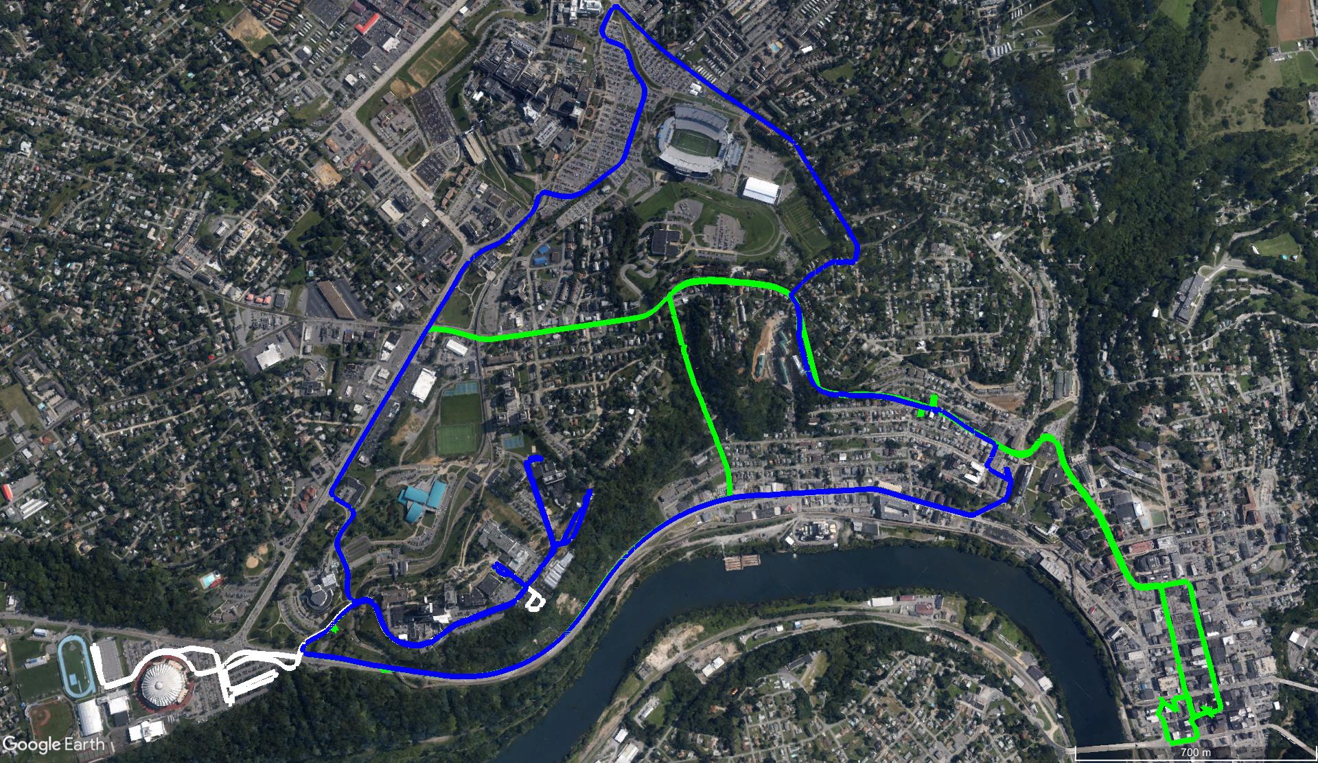
Figure 2: Ground trace for the three utilized GNSS data sets. The white trace corresponds to data collect 1, the green trace corresponds to data collect 2, and the blue trace corresponds to data collect 3.

For these data collects, the binary in-phase and quadrature (IQ) data in the L1-band was recorded. By recording the IQ data in place of the GNSS receiver dependent observations (i.e., the pseudorange and carrier-phase observables), the same data collect can be utilized to generate several sets of observations with varying levels of degradation after playing back through a software defined GNSS receiver [29] with different sets of tracking parameters. Specifically, the receiver dependent observations can be generated off-line by playing the IQ data into a GNSS receiver, where the level of degradation is varied by changing the GNSS receiver’s tracking parameters (i.e., changing the bandwidth of the phase lock loop (PLL), the delay lock loop (DLL) and the correlator spacing). For a detailed discussion on the impact that the GNSS receiver tracking parameters can have on the quality of the generated observables, the reader is referred to [30, 31], which is reviewed in [5].

For this study, two sets of observations are generated (i.e., a low-quality and high-quality data set) for each of the data collects. The specific GNSS receiver tracking parameters utilized to generate the low-quality and high-quality observations are provided within Table III of [5]

IV-B Evaluation

Utilizing these data collects, an evaluation of the proposed methodology can be conducted. To provided a comparison for the proposed approach, three additional estimation frameworks will be utilized. The first comparison methodology is the traditional $l^{2}\text{-norm}$ based estimator. The second comparison methodology is the MM approach, which has a static measurement error covariance model (i.e., a fixed two component measurement error covariance model). The final comparison methodology is the DCS approach, where the DCS approach is utilized because it is both a closed form version of switchable constraints and a specific implementation of an m-estimator [8]. All of the utilized estimators are built upon the iSAM2 algorithm [11], as implemented within the Georgia Tech Smoothing and Mapping (GTSAM) library [32].

IV-B1 Localization Performance

To start an evaluation, the localization performance of the estimation frameworks will be assessed. To enable the assessment of the localization performance, a reference ground-truth must first be established. To generate this ground-truth, a differential GNSS solution (i.e., real time kinematic (RTK)) is utilized, which is known to provide centimeter level localization accuracy [30].

With the RTK generated reference ground-truth solution, the localization performance of the four estimation frameworks, when low-quality observations are utilized, is provided in Table I(c). From Table I(c), it can be seen that all three of the robust estimation frameworks provided a significant increase is localization accuracy, with respect to the median, when compared to the traditional $l^{2}\text{-norm}$ approach. Additionally, it should be noted that the ICE approach provides the most accurate solution for all three data collects when low-quality observations are utilized.

TABLE I: Horizontal RSOS localization error results when low fidelity receiver tracking parameters are utilized to generate the observations. The green and red cell entries correspond to the minimum and maximum statistic, respectively.

(a) Localization results for data collect 1.

(m.)	$L_{2}$	DCS	MM	ICE
mean	2.51	0.99	1.66	0.73
median	2.57	0.64	1.63	0.56
std. dev.	1.41	0.98	1.05	0.72
max	10.78	9.71	10.06	13.19

(b) Localization results for data collect 2.

(m.)	$L_{2}$	DCS	MM	ICE
mean	4.00	4.00	3.12	2.11
median	2.48	2.08	1.94	0.93
std. dev.	3.87	4.59	3.92	2.10
max	29.18	31.05	31.40	23.02

(c) Localization results for data collect 3.

(m.)	$L_{2}$	DCS	MM	ICE
mean	4.94	4.16	4.51	4.35
median	4.41	2.82	3.62	1.48
std. dev.	2.97	3.54	3.33	5.23
max	29.53	30.38	28.30	26.61

TABLE II: Horizontal RSOS localization error results when high fidelity receiver tracking parameters are utilized to generate the observations. The green and red cell entries correspond to the minimum and maximum statistic, respectively.

(a) Localization results for data collect 1.

(m.)	$L_{2}$	DCS	MM	ICE
mean	0.44	0.43	0.41	0.42
median	0.37	0.36	0.35	0.35
std. dev.	0.30	0.27	0.29	0.28
max	5.38	5.33	5.35	5.22

(b) Localization results for data collect 2.

(m.)	$L_{2}$	DCS	MM	ICE
mean	0.79	0.81	0.84	0.79
median	0.82	0.81	0.84	0.83
std. dev.	0.46	0.46	0.50	0.46
max	3.97	3.93	10.77	2.95

(c) Localization results for data collect 3

(m.)	$L_{2}$	DCS	MM	ICE
mean	1.09	1.10	1.11	1.07
median	0.96	0.95	1.00	0.89
std. dev.	0.67	0.73	0.72	0.66
max	7.83	7.83	18.08	7.82

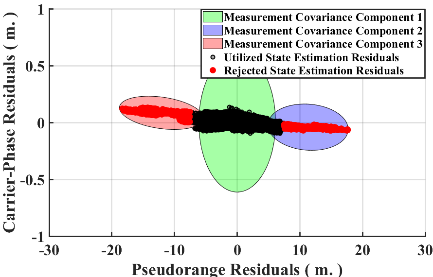
(a) Incrementally estimated measurement error covariance model for data collect 1. For this measurement uncertainty model, approximately 91% of the observations are characterized by component 1.

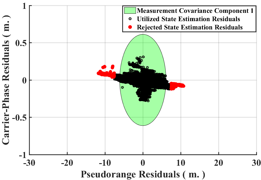
(b) Incrementally estimated measurement error covariance model for data collect 2. For this data collect, only 249 observations did not adhere to the a priori measurement uncertainty model.

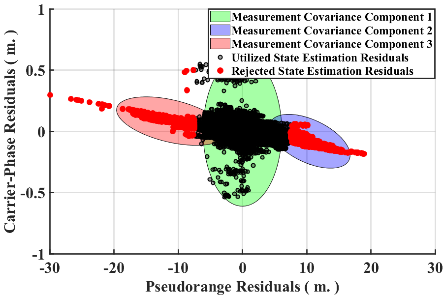
(c) Incrementally estimated measurement error covariance model for data collect 3. For this measurement uncertainty model, approximately 98% of the observations are characterized by component 1.

Figure 3: Incrementally estimated measurement error covariance model when the observations are generated with high fidelity receiver tracking parameters.

To continue the localization performance evaluation, we can assess the localization performance of the four estimation frameworks with the high-quality observations, as provided in Table II(c). From Table II(c), first, it should be noted that all four estimation frameworks are providing comparable localization statistics – as would be expected when the utilized observations adhere to the a priori measurement error covariance model. However, it can also be noted that the ICE approach is providing the most accurate localization statistics the majority of the time.

IV-B2 Covariance Estimation Analysis

To continue the evaluation, the estimated covariance from the ICE approach is assessed. Within this assessment, we have two primary objectives. First, we would like to show that the incrementally estimated covariance represents the measurement uncertainty model. Secondly, we would like to show that the covariance estimation process is efficiently conducted.

To enable this assessment the high-quality observations are utilized, as provided in Fig. 3. Within Fig. 3, the black points correspond to the state estimation residuals of observations which sufficiently adhere to the a priori measurement error uncertainty model. While, the red points correspond to the state estimation residuals of observations which were not well defined by the a priori measurement uncertainty model, and thus not included during optimization; however, were utilized to modify the measurement uncertainty model. Additionally, the ellipses correspond to components of the incrementally estimated measurement error uncertainty model, with $95$% confidence.

From Fig. 3, it can be seen that the incrementally estimated measurement uncertainty models closely resemble the assumed model for the high quality observations (i.e., an inlier distribution which characterizes a majority of the observations, and outlier distributions which characterize a small percentage of erroneous observations). This is specifically evident for data collects 1 and 3, as depicted in Fig. 3(a) and Fig. 3(c), respectively.

To verify the efficiency of the covariance adaptation approach, we can evaluate the number of times the measurement uncertainty model was adapted. For, data collects 1 and 3, as depicted in Fig, 3(a) and Fig. 3(c), the covariance model was only adapted once to enable the incorporation of two outlier distributions. For data collect 2, as depicted in Fig. 3(b), no covariance adaptation step was conducted – instead, only $249$ observations were rejected. In contrast, if the covariance model was naively adapted every time the number of residuals were greater than the residual cardinality threshold, then data collect 1 would have required 75 adaptations, data collect 2 would have required 57 adaptations, and data collect 3 would have required 91 adaptations. Thus, the incorporation of the $\operatorname{z-test}$ to partition the set of residuals dramatically increased the efficiency of the proposed approach.

IV-B3 Run-time Analysis

To conclude the evaluation of the proposed methodology, a run-time comparison is provided in Fig 4. From Fig. 4, it is shown that $l^{2}\text{-norm}$, DCS, and the MM approaches all provide comparable run-time performance.

Additionally, it is clearly shown that the ICE methodology, provides the slowest average run-time; however, this slower run-time – which is still on average approximately $25\ \text{Hz}$ – could prove to be a valid comprise when considering the significantly increase in localization accuracy granted by the approach.

Finally, although the ICE approach does currently provide the slowest run-time, an additional points should be made. For the current ICE implementation, the primary run-time bottle-neck for the current evaluation is implementation based. Specifically, the ICE algorithm could be implemented in such a way to dramatically decrease run-time by simply parallelizing the covariance adaptation and state estimation steps.

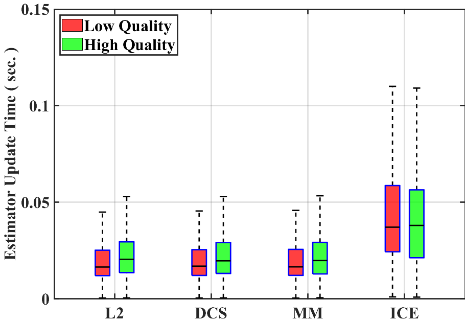
Figure 4: Estimator update time for each of the estimation frameworks over all data collects, where $L2$ is a batch estimator with $l^{2}\text{-norm}$ cost function, DCS is the dynamic covariance scaling robust estimator, MM is the max-mixtures approach with a static measurement covariance model, and ICE is the proposed incremental covariance estimation technique.

V Conclusion

Within this paper, we propose a novel extension to the measurement uncertainty model estimation paradigm for enabling robust state estimation. Specifically, we propose an efficient, incremental extension of the methodology. The efficiency of the approach is granted by adapting the uncertainty model with only a small subset of informative state estimation residuals (i.e., the state estimation residuals which do not adhere to the a priori model). The incremental nature of the approach is granted through recent advances within the probabilistics graphical model community, and the ability to merge GMM’s.

To evaluate the proposed ICE approach, three degraded GNSS data sets are utilized. Based upon the results obtained on these data sets, the proposed approach provides promising results. Specifically, the proposed ICE approach provides significantly increased localization performance when utilizing degraded data, when compared to other state-of-the-art robust, incremental estimation algorithms.

References

- [1] D. Simon, Optimal state estimation: Kalman, H infinity, and nonlinear approaches. John Wiley & Sons, 2006.
- [2] R. E. Kalman, “A new approach to linear filtering and prediction problems,” Journal of basic Engineering, vol. 82, no. 1, pp. 35–45, 1960.
- [3] S. Thrun, W. Burgard, and D. Fox, Probabilistic robotics. MIT press, 2005.
- [4] F. R. Hampel, “Contribution to the theory of robust estimation,” Ph. D. Thesis, University of California, Berkeley, 1968.
- [5] R. M. Watson, J. N. Gross, C. N. Taylor, and R. C. Leishman, “Enabling Robust State Estimation through Measurement Error Covariance Adaptation,” IEEE Transactions on Aerospace and Electronic Systems, pp. 1–1, 2019.
- [6] P. J. Huber, Robust Statistics. Wiley New York, 1981.
- [7] N. Sünderhauf and P. Protzel, “Switchable constraints for robust pose graph SLAM,” in 2012 IEEE/RSJ International Conference on Intelligent Robots and Systems, pp. 1879–1884, IEEE, 2012.
- [8] P. Agarwal, G. D. Tipaldi, L. Spinello, C. Stachniss, and W. Burgard, “Robust map optimization using dynamic covariance scaling,” in 2013 IEEE International Conference on Robotics and Automation, pp. 62–69, Citeseer, 2013.
- [9] E. Olson and P. Agarwal, “Inference on networks of mixtures for robust robot mapping,” The International Journal of Robotics Research, vol. 32, no. 7, pp. 826–840, 2013.
- [10] T. Pfeifer and P. Protzel, “Incrementally learned mixture models for gnss localization,” arXiv preprint arXiv:1904.13279, 2019.
- [11] M. Kaess, H. Johannsson, R. Roberts, V. Ila, J. J. Leonard, and F. Dellaert, “iSAM2: Incremental smoothing and mapping using the Bayes tree,” The International Journal of Robotics Research, vol. 31, no. 2, pp. 216–235, 2012.
- [12] M. Song and H. Wang, “Highly efficient incremental estimation of Gaussian mixture models for online data stream clustering,” in Intelligent Computing: Theory and Applications III, vol. 5803, pp. 174–184, International Society for Optics and Photonics, 2005.
- [13] F. Dellaert, M. Kaess, et al., “Factor graphs for robot perception,” Foundations and Trends® in Robotics, vol. 6, no. 1-2, pp. 1–139, 2017.
- [14] R. M. Watson and J. N. Gross, “Evaluation of kinematic precise point positioning convergence with an incremental graph optimizer,” in Position, Location and Navigation Symposium (PLANS), 2018 IEEE/ION, pp. 589–596, IEEE, 2018.
- [15] J. R. Blair and B. Peyton, “An introduction to chordal graphs and clique trees,” in Graph theory and sparse matrix computation, pp. 1–29, Springer, 1993.
- [16] F. Dellaert and M. Kaess, “Square Root SAM: Simultaneous localization and mapping via square root information smoothing,” The International Journal of Robotics Research, vol. 25, no. 12, pp. 1181–1203, 2006.
- [17] G. J. Bierman, Factorization Methods for Discrete Sequential Estimation (Dover Books on Mathematics). Dover Publication, 2006.
- [18] M. Kaess, A. Ranganathan, and F. Dellaert, “Fast Incremental Square Root Information Smoothing.,” in IJCAI, pp. 2129–2134, 2007.
- [19] G. H. Golub and C. F. van Loan, Matrix Computations. JHU Press, fourth ed., 2013.
- [20] M. Kaess, V. Ila, R. Roberts, and F. Dellaert, “The Bayes tree: An algorithmic foundation for probabilistic robot mapping,” in Algorithmic Foundations of Robotics IX, pp. 157–173, Springer, 2010.
- [21] Z. Zhang, “Parameter estimation techniques: A tutorial with application to conic fitting,” Image and vision Computing, vol. 15, no. 1, pp. 59–76, 1997.
- [22] R. M. Watson and J. N. Gross, “Robust Navigation In GNSS Degraded Environment Using Graph Optimization,” in Proceedings of the 30th International Technical Meeting of The Satellite Division of the Institute of Navigation (ION GNSS+2017), pp. 2906–2918, 2017.
- [23] D. M. Blei, M. I. Jordan, et al., “Variational inference for Dirichlet process mixtures,” Bayesian analysis, vol. 1, no. 1, pp. 121–143, 2006.
- [24] M. Beal, Variational algorithms for approximate Bayesian inference. PhD thesis, University of London, 2003.
- [25] D. Steinberg, An unsupervised approach to modelling visual data. PhD thesis, University of Sydney., 2013.
- [26] A. Doucet and X. Wang, “Monte Carlo methods for signal processing: a review in the statistical signal processing context,” IEEE Signal Processing Magazine, vol. 22, no. 6, pp. 152–170, 2005.
- [27] O. Ledoit, M. Wolf, et al., “Some hypothesis tests for the covariance matrix when the dimension is large compared to the sample size,” The Annals of Statistics, vol. 30, no. 4, pp. 1081–1102, 2002.
- [28] H. Hotelling, “The generalization of Student’s ratio,” in Breakthroughs in statistics, pp. 54–65, Springer, 1992.
- [29] C. Fernandez-Prades, J. Arribas, P. Closas, C. Aviles, and L. Esteve, “GNSS-SDR: an open source tool for researchers and developers,” in Proceedings of the 24th International Technical Meeting of The Satellite Division of the Institute of Navigation (ION GNSS 2011), pp. 780–0, 2001.
- [30] E. Kaplan and C. Hegarty, Understanding GPS: principles and applications. Artech house, 2005.
- [31] A. Van Dierendonck, P. Fenton, and T. Ford, “Theory and performance of narrow correlator spacing in a gps receiver,” Navigation, vol. 39, no. 3, pp. 265–283, 1992.
- [32] F. Dellaert, “Factor graphs and gtsam: A hands-on introduction,” tech. rep., Georgia Institute of Technology, 2012.
- [33] T. Takasu, “RTKLIB: An open source program package for GNSS positioning,” 2011.